Response theory for time-resolved second-harmonic generation
and two-photon photoemission

Abstract

A unified response theory for the time-resolved nonlinear light generation and two-photon photoemission (2PPE) from metal surfaces is presented. The theory allows to describe the dependence of the nonlinear optical response and the photoelectron yield, respectively, on the time dependence of the exciting light field. Quantum-mechanical interference effects affect the results significantly. Contributions to 2PPE due to the optical nonlinearity of the surface region are derived and shown to be relevant close to a plasmon resonance. The interplay between pulse shape, relaxation times of excited electrons, and band structure is analyzed directly in the time domain. While our theory works for arbitrary pulse shapes, we mainly focus on the case of two pulses of the same mean frequency. Difficulties in extracting relaxation rates from pump-probe experiments are discussed, for example due to the effect of detuning of intermediate states on the interference. The theory also allows to determine the range of validity of the optical Bloch equations and of semiclassical rate equations, respectively. Finally, we discuss how collective plasma excitations affect the nonlinear optical response and 2PPE.

I Introduction

During the last decade time-resolved spectroscopy of condensed-matter systems has become a very active area of experimental research Ste92 ; HMKB97 ; Sim98 ; KSR98 ; Gud99 ; Schoe ; Aesch1 ; Aesch2 ; Wolf1 ; Hoef97 ; Cao97 ; Petek ; Wolf2 ; Leh99 ; Kno00 ; GWH00 ; SBW02 ; ONP02 ; Gerb ; Ae.cluster ; Petekrev ; Fausterrev . This is mainly due to the progress in experimental technique, in particular the ability to create ultra-short laser pulses with a duration of the order of a few femtoseconds femto . Since this is similar to the relaxation times of excited electrons and collective excitations in solids, these experiments allow to study non-equilibrium physics, e.g., the time evolution of excited electrons before and during thermalization. Of particular interest are non-linear techniques such as time-resolved sum-frequency generation (SFG) and two-photon photoemission (2PPE), which are sensitive to excited electron states Shen . A theoretical understanding of these processes is crucial. Petek and Ogawa Petekrev noted in 1997 that a theory for time-resolved 2PPE is still lacking, and, despite the efforts of many theorists, much remains to be done. The situation for SFG is similar. The construction of such a theory is a formidable task—the main problems are (a) the desription of the time-dependent response and (b) the treatment of the surface. Our main concern is with the first point. A simplified description of the surface using Fresnel factors has been employed successfully to describe SFG from metals SMD87 ; HBB94 ; Luce97 ; LuceLDA . A detailed discussion of boundary conditions at the surface, focusing on the nonlinear optical response of magnetic systems, can be found in Ref. AtK02 .

In the present paper we discuss the electronic processes taking place during time-resolved SFG (in particular second-harmonic generation, SHG) and 2PPE and derive the dependence of the SFG light intensity and the 2PPE photoelectron yield on the time dependence of the exciting laser field. We show that most effects observed for time-resolved 2PPE appear similarly for SFG, such as their dependence on energy relaxation, dephasing, and detuning of intermediate states. Other examples are the enhancement of the response due to collective excitations and the sensitivity regarding the ultra-fast spin-dependent relaxation. We develop a unified time-dependent response theory for SFG and 2PPE, starting from the self-consistent field approach of Ehrenreich and Cohen EC ; HB , which can be applied to specific materials described by their band structure, relaxation rates, and dipole matrix elements. For illustration, we apply the theory to a generic tight-binding model for a metal to study interference effects in both pump-probe single-color SFG and 2PPE and their dependence on relaxation rates and detuning. We exhibit the strong similarities between both methods.

Figure 1: Simplified representation of sum-frequency generation (SFG). $E_{F}$ is the Fermi energy and $E_{\mathrm{vac}}$ is the vacuum energy. In SFG two photons of frequencies $\omega_{1}$ and $\omega_{2}$ are absorbed by electrons in states $|1\rangle$ and $|2\rangle$ and a single photon of frequency $\omega_{1}+\omega_{2}$ is emitted due to the electronic transition $|3\rangle\to|1\rangle$. The two photons may be provided by one or two laser pulses. Note, whether the two photons are predominantly absorbed at nearly the same time or with some delay depends on the shape and width of the pulse(s). A more careful analysis of the absorption process on the basis of response theory is given in Sec. II.1.

In SFG Ste92 ; HMKB97 ; Sim98 ; KSR98 ; Gud99 electrons are excited by absorbing two photons and they subsequently emit a single photon at the sum frequency. In Fig. 1 we illustrate the type of process yielding SFG. For simplicity we talk about SFG in the following, although difference-frequency generation is automatically included in our theory. Time-resolved measurements Ste92 ; HMKB97 ; Sim98 ; KSR98 ; Gud99 usually employ the pump-probe technique, where two laser pulses of the same (single-color) or different (two-color) frequency are applied with a time delay $\Delta T$ between them. This time delay controls the time between the two absorptions and thus the relaxation dynamics of the electron in the intermediate state $|2\rangle$ is crucial, see Fig. 1. SFG is strongly surface-sensitive, since the SFG response of the bulk of an inversion-symmetric crystal vanishes in the dipole approximation. The inversion symmetry can also be broken by nanostructures. The most important case of SFG is second-harmonic generation (SHG), where the electrons are excited by approximately monochromatic light of frequency $\omega$ and light of frequency $2\omega$ is detected. Note, in the case of ultra-short laser pulses the spectrum is necessarily broadened and a full treatment of SFG is required even for these single-color experiments. Also note that a single laser pulse, depending on its duration and shape, involves time-delayed absorptions.

Time-resolved 2PPE experiments of metal surfaces Schoe ; Aesch1 ; Aesch2 ; Wolf1 ; Hoef97 ; Cao97 ; Petek ; Wolf2 ; Leh99 ; Kno00 ; GWH00 ; SBW02 ; ONP02 as well as of clusters Gerb ; Ae.cluster employing the pump-probe technique have been performed more often than time-resolved SFG. Reviews can be found in Refs. Petekrev and Fausterrev . Figure 2 shows a sketch of the processes yielding 2PPE. An electron is excited above the vacuum energy $E_{\mathrm{vac}}$ due to the absorption of two photons. The interplay between the relaxation of the electrons in intermediate states and the time between the two absorptions will determine the resulting photoelectron current. The probability of electrons above the vacuum level actually leaving the solid is also crucial. The limited mean free path of the electrons makes photoemission surface-sensitive, but in general less than in the case of SFG. In both SFG and 2PPE interference effects Ste92 ; Sim98 ; Aesch2 ; Cao97 ; Petek ; Wolf2 appear, which our theory allows to study. Of course, these interference effects are expected to depend on the pulse shapes.

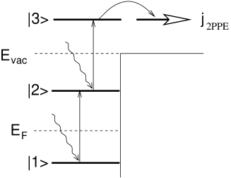
Figure 2: Simplified representation of two-photon photoemission (2PPE), where $E_{F}$ is the Fermi energy and $E_{\mathrm{vac}}$ the vacuum energy. Here, two photons of frequencies $\omega_{1}$ and $\omega_{2}$ (out of the same or different pulses) are absorbed by electrons in states $|1\rangle$ and $|2\rangle$, respectively. Compared to SFG, Fig. 1(a), the excitation energy is now so large that electrons are excited above $E_{\mathrm{vac}}$ and can leave the solid. The open arrow denotes electrons leaving the crystal. Note, SFG is also possible due to a transition $|3\rangle\to|1\rangle$. However, the SFG intensity may be small, since it involves more dipole matrix elements, as we discuss below.

The response theory presented here goes beyond previous theoretical treatments of ultra-fast processes rem.slow in SFG and 2PPE in metals, which mainly fall into four classes: (a) density functional theory and approaches based thereon Lie89 ; Ull97 ; LuceLDA ; Lie99 ; Koh99 ; WDS ; Camp , (b) rate equations Kno00 ; Rol1 ; Rol2 , (c) optical Bloch equations Wolf1 ; Petek ; Loudon , and (d) perturbative methods HB ; HBB94 ; PPK00 ; Sha00 . At first, density functional theory has been applied in the time-dependent local-density approximation for jellium models Lie89 ; Ull97 ; Lie99 ; Koh99 . In the jellium approximation one ignores the potential of the ion cores and, consequently, any band-structure effects. Thus this approach is not suitable if single bands or surface states or quantum-well states in thin films are important. On the other hand, collective excitations are usually described rather well Lieplas . Going beyond the jellium model, Luce and Bennemann have employed the local density approximation to calculate dipole matrix elements as they enter also in our approach LuceLDA . Additionally taking excited states into account within the GW approximation, Schöne et al. WDS have calculated electronic lifetimes. Hole dynamics have also been studied with density functional methods Camp .

However, one would like to gain more general physical insight than the numerical results can provide. To this end one may consider rate equations for the occupation of excited states, e.g., the Boltzmann equation Kno00 ; Rol1 ; Rol2 . This approach allows to incorporate important effects such as secondary electrons due to relaxation from higher-energy states and to Auger processes as well as transport into the bulk Kno00 ; Rol1 ; Rol2 . However, rate equations neglect the electric polarization of the electron gas, its dephasing, and any quantum-mechanical interference effects, resulting from the superposition of the laser field and the induced fields. To include these effects one has to solve the equation of motion for the entire density matrix $\rho$, not only for its diagonal components, i.e., the occupations. This can be done in response theory. Its simplest form yields the optical Bloch equations: The system is modelled by a small number of levels and the von Neumann equation of motion (master equation) for the density matrix is integrated numerically Loudon ; Wolf1 ; Petek . However, this approach is limited to a small number of levels so that a realistic band structure cannot be described. Furthermore, many-particle effects like collective excitations are not included.

On the other hand, the response theory presented here does include the band structure and collective excitations. It generalizes the theory of Hübner and Bennemann HB to SFG due to incident light of arbitrary time dependence and spectrum. The previous theory HB has been used successfully for SHG from metal surfaces, thin films, quantum wells, and metallic monolayers due to continuous-wave, monochromatic light HB ; HBB94 ; Luce97 ; LuceLDA ; NOLI ; Luce96 ; Luce98 ; AnH02 . However, the dependence of SHG on the pulse shape and the effect of energy relaxation and dephasing were not discussed. We also derive the response expressions for time-dependent 2PPE within the same framework. Since our theory is explicitly formulated for continuous bands, it can also serve as a basis for the discussion of the averaging effects due to bands of finite width discussed in a more heuristic framework using optical Bloch equations for discrete levels in Ref. Weida . Since the full time or frequency dependence is included, effects of frequency broadening of short pulses and of finite frequency resolution of the detector (for SFG) Weida are easily studied.

Our theory employs a generalized self-consistent-field approach EC ; HB , which is equivalent to the random-phase approximation (RPA) Dasgupta ; Lind54 ; HG70 ; Ch98 ; Mahan . We employ the electric-dipole approximation, which is valid for small wave vector ${\bf q}$ of the electromagnetic field and has been used successfully to describe SHG from metal surfaces HBB94 ; Luce97 ; LuceLDA ; NOLI ; Luce96 ; Luce98 ; AnH02 ; Shala . This is reasonable, since the skin depth, which is the length scale of field changes, is about one order of magnitude larger than the lattice constant. One has to take care in interpreting SFG experiments for inversion-symmetric crystals, since the surface contribution only dominates over higher multipole bulk contributions for surfaces of low symmetry HBB94 ; HB . Similar in spirit to our response theory, Ueba Ueba has studied continuous-wave 2PPE from metal surfaces, Pedersen et al. PPK00 have considered continous-wave SHG from metallic quantum wells, and Shahbazyan and Perakis Sha00 have developed a time-dependent, but linear response theory for metallic nanoparticles.

It is important to understand that at the surface of a metal, in thin films, and in nanostructures the light couples to collective plasma excitations. The field within the metal is of course not purely transverse Barton ; Board . Its transverse and longitudinal components couple with the conduction electrons to form plasmon-polaritons and plasmons, respectively Board . The (longitudinal) plasmon modes only decouple from the applied field for a structureless jellium model of the solid Barton ; Board . However, we consider a more realistic model that incorporates the crystal structure. Also, we will see that the induced nonlinear polarization couples to (longitudinal) plasmon modes.

On general grounds one may expect that the discussion of the intimate relationship between 2PPE and SFG also helps to understand the dependence of 2PPE on light polarization. It has been shown that the light-polarization dependence of SFG is important for the analysis of the electronic structure and magnetism Oxf .

The organization of the remainder of this paper is as follows: We first summarize the response theory for SFG and 2PPE in Sec. II. This lays the ground for our discussion in Sec. III of time-dependent SFG and 2PPE. Details of the response theory are given in appendices A and B.

II Response theory

II.1 Sum-frequency generation

We first outline the response theory for SFG. We consider a semi-infinite solid with single-particle states $|{\bf k}_{\|}l\rangle$ with energies $E_{{\bf k}_{\|}l}$ described by the momentum ${\bf k}_{\|}$ parallel to the surface, which is assumed to be perpendicular to the $z$ direction, and a set of additional quantum numbers $l$. For bulk states, which may be affected by the surface but are not localized close to it, the composite band index is $l=(k_{z},\nu,\sigma)$, where $k_{z}$ is the $z$ momentum component in the bulk, $\nu$ is a band index, and $\sigma$ is the spin quantum number. $k_{z}$ has a continuous spectrum. On the other hand, for states localized at the surface, $l$ is discrete. Examples are image-potential states, adsorbate states, quantum-well states in a thin overlayer, and proper surface states.

Part of the electron-electron interaction is included by the self-consistent-field approximation or RPA EC ; Dasgupta . The remaining electron-electron scattering is approximately taken into account by inserting phenomenological relaxation rates PS00 into the single-electron Green functions and by shifting the band energies $E_{{\bf k}_{\|}l}$ Louisell . We assume that $E_{{\bf k}_{\|}l}$ are quasiparticle energies containing these shifts. Note, the electron-phonon interaction only becomes relevant on longer time scales and is not considered here rem.slow . Also, intraband contributions to the response are not considered for simplicity, which is reasonable at optical frequencies.

The electrons are coupled to the effective electric field ${\bf E}$ within the solid through a dipolar interaction term (for simplicity we assume that the dipole coupling dominates). The optically induced polarization ${\bf P}$ within the solid is expanded in orders of the electric field ${\bf E}$. The linear response is given by

$$P_{i}^{(1)}({\bf q},t)=\frac{1}{2\pi}\sum_{q^{\prime}_{z}}\int dt^{\prime}\>\chi_{ij}({\bf q},{\bf q}^{\prime};t-t^{\prime})\,E_{j}({\bf q}^{\prime},t^{\prime}),$$ (1)

where $\chi_{ij}$ is the linear susceptibility, ${\bf q}=({\bf q}_{\|},q_{z})$, and ${\bf q}_{\|}={\bf q}^{\prime}_{\|}$ due to conservation of momentum parallel to the surface. Summation over repeated indices is always implied. The non-conservation of $q_{z}$ is explicitly taken into account.

We assume throughout that the photon momentum ${\bf q}$ is small compared to the dimensions of the Brillouin zone and that the band energies, relaxation rates, and transition matrix elements change slowly with momentum so that the difference between the parallel crystal momentum of an electron before and after the interaction, ${\bf k}_{\|}$ and ${\bf k}_{\|}^{\prime}$, respectively, can be ignored. If we further neglect the frequency dependence of the transition matrix elements the self-consistent-field approach gives the time-dependent linear susceptibility

$$\chi_{ij}({\bf q},{\bf q}^{\prime};t-t^{\prime})=\frac{e^{2}}{v}\frac{2\pi i}{\hbar}\,\Theta(t-t^{\prime})$$ (2)

$$\quad{}\times\sum_{{\bf k}_{\|}}\sum_{ll^{\prime}}D^{i}_{{\bf k}_{\|}l^{\prime};{\bf k}_{\|}l}(-q_{z})\,D^{j}_{{\bf k}_{\|}l;{\bf k}_{\|}l^{\prime}}(q_{z}^{\prime})\>$$

$$\quad{}\times[f(E_{{\bf k}_{\|}l^{\prime}})-f(E_{{\bf k}_{\|}l})]\,\exp\!\left[i\frac{E_{{\bf k}_{\|}l^{\prime}}-E_{{\bf k}_{\|}l}}{\hbar}(t-t^{\prime})\right]$$

$$\quad{}\times\exp[-\Gamma_{{\bf k}_{\|}l;{\bf k}_{\|}l^{\prime}}(t-t^{\prime})],\!$$

where ${v}$ is the volume of the system. Note, the last two factors explicitly describe the oscillations and decay of the linear induced polarization. In the dipole approximation the transition matrix elements are

$${\bf D}_{{\bf k}_{\|}l;{\bf k}_{\|}l^{\prime}}(q_{z})\equiv\langle{\bf k}_{\|}l|\,{\bf r}\,|{\bf k}_{\|}l^{\prime}\rangle.$$ (3)

The matrix elements are given without approximations in App. A. The linear susceptibility is represented by the usual Feynman diagram shown in Fig. 3.

Figure 3: The Feynman diagram for the linear susceptibility $\chi$ relating the linear polarization ${\bf P}^{(1)}$ to the effective electric field ${\bf E}$, cf. Eq. (1). The solid lines in the diagrams are to be understood as electronic Matsubara-Green functions containing relaxation rates $\Gamma$. The dots ($\bullet$) denote dipole matrix elements $\mathbf{D}$.

The finite lifetime of electrons due to their interaction enters Eq. (2) through the dephasing rates $\Gamma_{{\bf k}_{\|}l;{\bf k}^{\prime}_{\|}l^{\prime}}$, which describe the decay of the superposition of states $|{\bf k}_{\|}l\rangle$ and $|{\bf k}^{\prime}_{\|}l^{\prime}\rangle$ and thus of the polarization. The change of the occupation of states is described by the energy relaxation rates $\Gamma_{{\bf k}_{\|}l;{\bf k}_{\|}l}\equiv\tau_{{\bf k}_{\|}l}^{-1}$, where $\tau_{{\bf k}_{\|}l}$ are the lifetimes. $\Gamma_{{\bf k}_{\|}l;{\bf k}_{\|}l}$ is the rate of spontaneous transitions out of the state $|{\bf k}_{\|}l\rangle$. Since the depopulation of the states $|{\bf k}_{\|}l\rangle$ or $|{\bf k}^{\prime}_{\|}l^{\prime}\rangle$ certainly leads to the destruction of the polarization, the dephasing rates can be expressed in terms of the lifetimes as Louisell

$$\Gamma_{{\bf k}_{\|}l;{\bf k}^{\prime}_{\|}l^{\prime}}=\frac{\tau_{{\bf k}_{\|}l}^{-1}+\tau_{{\bf k}^{\prime}_{\|}l^{\prime}}^{-1}}{2}+\Gamma^{\mathrm{ph}}_{{\bf k}_{\|}l;{\bf k}^{\prime}_{\|}l^{\prime}},$$ (4)

where $\Gamma^{\mathrm{ph}}$ describes additional dephasing.

The induced second-order polarization is given by

$$P_{i}^{(2)}(t)=\frac{1}{(2\pi)^{2}}\int dt_{1}\,dt_{2}\>\chi^{(2)}_{ijk}(t-t_{1},t_{1}-t_{2})\,E_{j}(t_{1})\,E_{k}(t_{2}).$$ (5)

The second-order susceptibility $\chi^{(2)}$ depends only on two time differences due to homogeneity in time. Obviously, $|t_{1}-t_{2}|$ is the time interval between the two absorptions. For a single laser pulse this interval is controlled by the pulse width. For two pulses we expect a contribution for $|t_{1}-t_{2}|$ of the order of the pump-probe delay time $\Delta T$. Note, the light polarization is characterized by the components $E_{j}$.

To express the electric field ${\bf E}$ within the solid in terms of the applied external light field ${\bf E}_{\mathrm{las}}$ and similarly the electric field ${\bf E}_{\mathrm{out}}$ of the outgoing light in terms of the polarization ${\bf P}$ one should employ Fresnel formulae, which are also of importance for the coupling of the light to collective excitations, as we discuss below. We do not present the Fresnel formulae here, since they can be found in the literature SMD87 ; HBB94 . See also Refs. Born75 ; Board for effective Fresnel factors for systems of several layers, such as the important case of a coupling prism separated from the metal by a thin layer of air or vacuum Otto . Of course, it would be of interest to repeat Fresnel’s analysis for SFG, in particular deducing phase shifts etc.

Equation (5) is the basis for time-dependent SFG. Clearly the pulse shape of the applied light described by $\mathbf{E}(t)$ affects the induced polarization $\mathbf{P}^{(2)}(t)$. Note, for simple pulse shapes (Gaussian, Lorentzian, rectangular) it is possible to evaluate the integrals in Eq. (5) further. The light polarization dependence is controlled by the symmetries of the tensor $\chi^{(2)}_{ijk}$. The symmetries of $\chi^{(2)}$ for magnetic and nonmagnetic crystals under monochromatic light have been discussed in Ref. Pan . They are determined by the symmetry operations that leave the particular surface invariant. These symmetry arguments are unchanged for general time dependence of the applied laser field.

The intensity of SFG light is $I^{(2)}(t)\propto[E^{(2)}_{\mathrm{out}}(t)]^{2}\propto[P^{(2)}(t)]^{2}$. So far, typical experiments do not resolve the time dependence of the intensity, but measure the time-integrated SFG yield

$${\cal I}^{(2)}\equiv\int dt\>I^{(2)}(t)\propto\int dt\>\left[E^{(2)}_{\mathrm{out}}(t)\right]^{2}\propto\int dt\>\left[P^{(2)}(t)\right]^{2}.$$ (6)

For simplicity we here sum over polarization directions.

Time-resolved SFG may be performed by measuring ${\cal I}^{(2)}(\Delta T)$ as a function of the time delay $\Delta T$ between the applied field pulses. Omitting surface effects (Fresnel factors) to emphasize the structure of the results, the yield can be written as

$${\cal I}^{(2)}(\Delta T)\propto\int dt\,dt_{1}\,dt_{2}\,dt_{3}\,dt_{4}\;\chi^{(2)}_{ijk}(t-t_{1},t_{1}-t_{2})$$ (7)

$$\quad{}\times\chi^{(2)}_{ilm}(t-t_{3},t_{3}-t_{4})\,E_{j}(t_{1})\,E_{k}(t_{2})\,E_{l}(t_{3})\,E_{m}(t_{4}),$$

which is of fourth order in the incoming light field and thus of second order in its intensity. As mentioned above, the typical time differences dominating the response are controlled by the delay $\Delta T$, besides the pulse durations.

It is useful to write the second-order polarization $\mathbf{P}^{(2)}$ also in frequency space,

$$P_{i}^{(2)}(\omega)=\int d\omega^{\prime}\,\chi^{(2)}_{ijk}(\omega,\omega^{\prime})\,E_{j}(\omega^{\prime})\,E_{k}(\omega-\omega^{\prime}),$$ (8)

where $\chi^{(2)}_{ijk}(t-t_{1},t_{1}-t_{2})=\int d\omega\,d\omega^{\prime}\,e^{-i\omega(t-t_{2})}\,e^{-i\omega^{\prime}(t_{2}-t_{1})}\,\chi^{(2)}_{ijk}(\omega,\omega^{\prime})$ or

$$\chi^{(2)}_{ijk}(\omega,\omega^{\prime})=\frac{1}{4\pi^{2}}\int dt\,dt^{\prime}\>e^{i\omega t}\,e^{i\omega^{\prime}t^{\prime}}\,\chi^{(2)}_{ijk}(t+t^{\prime},-t^{\prime}).$$ (9)

Note that we employ the convention of Eq. (8) in Ref. HB for the Fourier transformation. The frequency representation is better suited to discuss transition energies. ${\bf P}^{(2)}$ has components at the sum of two frequencies of the incoming light. Since the Fourier transform of the real electric field contains positive and negative frequencies, the difference frequency also appears.

If at the first step we ignore screening effects, then Eqs. (5) and (7) only contain the second-order irreducible susceptibility

$$\chi^{(2)}_{\mathrm{irr};ijk}({\bf q},{\bf q}_{1},{\bf q}_{2};t-t_{1},t_{1}-t_{2})=-\frac{e^{3}}{v}\left(\frac{2\pi i}{\hbar}\right)^{\!2}\Theta(t-t_{1})\,\Theta(t_{1}-t_{2})\sum_{{\bf k}_{\|}}\sum_{ll^{\prime}l^{\prime\prime}}\,D^{i}_{{\bf k}_{\|}l;{\bf k}_{\|}l^{\prime\prime}}(-q_{z})\,\Bigg{(}D^{j}_{{\bf k}_{\|}l^{\prime\prime};{\bf k}_{\|}l^{\prime}}(q_{1z})$$ (10)

$$\qquad{}\times D^{k}_{{\bf k}_{\|}l^{\prime};{\bf k}_{\|}l}(q_{2z})\,\left[f(E_{{\bf k}_{\|}l})-f(E_{{\bf k}_{\|}l^{\prime}})\right]\,\exp\!\left[i\frac{E_{{\bf k}_{\|}l}-E_{{\bf k}_{\|}l^{\prime}}}{\hbar}\,(t_{1}-t_{2})\right]\,\exp[-\Gamma_{{\bf k}_{\|}l^{\prime};{\bf k}_{\|}l}(t_{1}-t_{2})]$$

$$\quad{}-D^{j}_{{\bf k}_{\|}l^{\prime};{\bf k}_{\|}l}(q_{1z})\,D^{k}_{{\bf k}_{\|}l^{\prime\prime};{\bf k}_{\|}l^{\prime}}(q_{2z})\,\left[f(E_{{\bf k}_{\|}l^{\prime}})-f(E_{{\bf k}_{\|}l^{\prime\prime}})\right]\,\exp\!\left[i\frac{E_{{\bf k}_{\|}l^{\prime}}-E_{{\bf k}_{\|}l^{\prime\prime}}}{\hbar}\,(t_{1}-t_{2})\right]$$

$$\qquad{}\times\exp[-\Gamma_{{\bf k}_{\|}l^{\prime\prime};{\bf k}_{\|}l^{\prime}}(t_{1}-t_{2})]\Bigg{)}\exp\!\left[i\frac{E_{{\bf k}_{\|}l}-E_{{\bf k}_{\|}l^{\prime\prime}}}{\hbar}\,(t-t_{1})\right]\,\exp[-\Gamma_{{\bf k}_{\|}l^{\prime\prime};{\bf k}_{\|}l}(t-t_{1})],$$

which is derived in App. A. We neglect the photon momenta relative to the crystal momentum. This expression, which forms the basis of our discussion of SFG, goes beyond the one given in Ref. HB in that it is valid for a time-dependent and spatially varying laser field. Furthermore, it includes the transverse response explicitly. Equation (10) already exhibits the interplay between the time interval $|t_{1}-t_{2}|$ between absorptions, the photon frequencies, the dephasing times, and the transition frequencies.

Figure 4: Detailed quantum-mechanical interpretation of a process contributing to SFG. An electron is excited from a pure state $|\mathbf{k}_{\|}l\rangle$ in the Fermi sea to a superposition of states $|\mathbf{k}_{\|}l\rangle$ and $|\mathbf{k}_{\|}l^{\prime\prime}\rangle$ by the absorption of two photons. After the absorptions the excited electron returns to the original pure state by emission of a SFG photon at the sum frequency. The times of the absorptions and the emission are indicated. The heavy wavy lines denote superpositions resulting from the absorption of photons (indicated by thin wavy lines with arrows) at $t_{2}$ and $t_{1}$, while the black dots represent electrons in pure eigenstates.

We now discuss the physics contained in Eq. (10) with the help of Fig. 4. We consider the first of the two terms in Eq. (10). The interpretation of the second term is similar rem.term2 . The step functions incorporate the time ordering $t_{2}<t_{1}<t$ and thus guarantee causality. The system is in equilibrium until the first absorption at time $t_{2}$ creates a superposition of the two states $|{\bf k}_{\|}l\rangle$ and $|{\bf k}_{\|}l^{\prime}\rangle$, denoted by the wavy line in Fig. 4. This important physics is lost in the interpretation illustrated by Fig. 1. The Fermi functions make sure that one of the states is initially occupied and the other is empty. Let us say state $|{\bf k}_{\|}l\rangle$ is occupied. Since the system is in a superposition of two eigenstates, the polarization oscillates with the frequency $(E_{{\bf k}_{\|}l}-E_{{\bf k}_{\|}l^{\prime}})/\hbar$, as follows from the first exponential in the parentheses in Eq. (10). Such superpositions are described by the off-diagonal components of the density matrix rem.linear . The diagonal components denoting the occupation numbers of states are not changed by a single absorption. The superposition decays with the dephasing rate $\Gamma_{{\bf k}_{\|}l^{\prime};{\bf k}_{\|}l}$ associated with this transition, making it clear why the dephasing rates rather than the energy relaxation rates dominate the response. A second absorption at the later time rem.simul $t_{1}$ changes the state into a superposition of the originally occupied state and the state $|{\bf k}_{\|}l^{\prime\prime}\rangle$ with its own characteristic oscillation frequency $(E_{{\bf k}_{\|}l}-E_{{\bf k}_{\|}l^{\prime\prime}})/\hbar$ and dephasing rate. This oscillating polarization can emit a photon at that frequency. After the emission the electron is again in the pure eigenstate $|{\bf k}_{\|}l\rangle$. The nonlinear susceptibility in Eq. (10) contains a sum over many contributions of this type from different momenta and bands Weida . Note, the product of three dipole matrix elements appearing in $\chi^{(2)}_{\mathrm{irr}}$ is responsible for the surface sensitivity of SFG, since in inversion symmetric crystals the product of dipole matrix elements connecting three states vanishes except when inversion symmetry is explicitly broken, e.g., by the surface.

In frequency space the nonlinear susceptibility is given by

$$\chi^{(2)}_{\mathrm{irr};ijk}({\bf q},{\bf q}_{1},{\bf q}_{2};\omega,\omega^{\prime})=-\frac{e^{3}}{v}\sum_{{\bf k}_{\|}}\sum_{ll^{\prime}l^{\prime\prime}}$$ (11)

$${}\times\frac{D^{i}_{{\bf k}_{\|}l;{\bf k}_{\|}l^{\prime\prime}}(-q_{z})}{-\hbar\omega+E_{{\bf k}_{\|}l}-E_{{\bf k}_{\|}l^{\prime\prime}}-i\hbar\Gamma_{{\bf k}_{\|}l^{\prime\prime};{\bf k}_{\|}l}}$$

$${}\times\bigg{[}D^{j}_{{\bf k}_{\|}l^{\prime\prime};{\bf k}_{\|}l^{\prime}}(q_{1z})\,D^{k}_{{\bf k}_{\|}l^{\prime};{\bf k}_{\|}}(q_{2z})\,$$

$$\qquad{}\times\frac{f(E_{{\bf k}_{\|}l})-f(E_{{\bf k}_{\|}l^{\prime}})}{-\hbar\omega+\hbar\omega^{\prime}+E_{{\bf k}_{\|}l}\!-E_{{\bf k}_{\|}l^{\prime}}\!-i\hbar\Gamma_{{\bf k}_{\|}l^{\prime};{\bf k}_{\|}l}}$$

$$\quad{}-D^{j}_{{\bf k}_{\|}l^{\prime};{\bf k}_{\|}l}(q_{1z})\,D^{k}_{{\bf k}_{\|}l^{\prime\prime};{\bf k}_{\|}l^{\prime}}(q_{2z})\,$$

$$\qquad{}\times\frac{f(E_{{\bf k}_{\|}l^{\prime}})-f(E_{{\bf k}_{\|}l^{\prime\prime}})}{-\hbar\omega+\hbar\omega^{\prime}+E_{{\bf k}_{\|}l^{\prime}}\!-E_{{\bf k}_{\|}l^{\prime\prime}}\!-i\hbar\Gamma_{{\bf k}_{\|}l^{\prime\prime};{\bf k}_{\|}l^{\prime}}}\bigg{]}.$$

This shows that the contribution of intermediate (virtual) states falls off with the inverse of the initial-state energy plus the photon energy minus the intermediate state energy, i.e., with the inverse of the detuning. This is not related to the lifetime broadening, but is due to Heisenberg’s uncertainty principle, which allows energy conservation to be violated on short time scales. The frequency picture also allows to incorporate a weight factor to account for the frequency resolution of the detector Weida . It is of interest to note that Eq. (11) and Fig. 4 can also describe spin-selective electron excitations due to circularly polarized light. Including the electron spins our response theory and in particular Eq. (11) apply also to magnetic systems.

To prepare the analysis of the effect of collective plasma excitations on the nonlinear optical response we now include the screening of the electric fields. Screening enters in two ways: First, the effective field ${\bf E}$ within the solid is not identical to the external field because of linear screening, which is expressed by the Fresnel formulae SMD87 ; HBB94 ; Luce97 ; LuceLDA ; AtK02 containing the dielectric function $\varepsilon$, which can be determined in the RPA. Secondly, the second-order polarization ${\bf P}^{(2)}$ of the electron gas, which corresponds to a displacement of charge, leads to an additional electric field Jackson

$$E_{i}^{(2)}({\bf r})=\int d^{3}r^{\prime}\,\sum_{j}\left[\frac{3(r_{i}-r^{\prime}_{i})(r_{j}-r^{\prime}_{j})}{|{\bf r}-{\bf r}^{\prime}|^{5}}-\frac{\delta_{ij}}{|{\bf r}-{\bf r}^{\prime}|^{3}}-\frac{4\pi}{3}\,\delta_{ij}\,\delta({\bf r}-{\bf r}^{\prime})\right]\,P_{j}^{(2)}({\bf r}^{\prime}).$$ (12)

Fourier transformation leads to

$${\bf E}^{(2)}({\bf k},t)=-4\pi\,\hat{\bf k}\,\hat{\bf k}\cdot{\bf P}^{(2)}({\bf k},t),$$ (13)

where $\hat{\bf k}$ is the unit vector in the direction of ${\bf k}$. Thus only the component of ${\bf P}^{(2)}({\bf k},t)$ parallel to ${\bf k}$, i.e., its longitudinal part, is accompanied by an electric field $\mathbf{E}^{(2)}$ Jackson , which is also longitudinal. Note that a longitudinal component of the electric field and of the induced polarization generally exists even for a transverse applied external field for lattice models Barton ; Board , see Eq. (11).

Due to the linear polarizability of the solid the additional field $\mathbf{E}^{(2)}$ leads to a polarization contribution of the form $\chi\mathbf{E}^{(2)}$. Since the field $\mathbf{E}^{(2)}$ in Eq. (13) is of second order in the applied field, see Eq. (5), this polarization contribution must be taken into account in $\mathbf{P}^{(2)}$. Doing this selfconsistently corresponds to the summation of an RPA series HB , as shown in App. A. Then, $P_{i}^{(2)}\propto\int dt_{1}\,dt_{2}\,\chi^{(2)}_{ijk}\,E_{j}\,E_{k}$ where now the nonlinear susceptibility $\chi^{(2)}_{ijk}$ obtains an additional factor and is given by

$$\chi^{(2)}_{ijk}({\bf q},{\bf q}_{1},{\bf q}_{2};t-t_{1},t_{1}-t_{2})=\frac{1}{2\pi}\sum_{m}\sum_{\tilde{\bf q}}\int d\tilde{t}$$ (14)

$$\quad{}\times\varepsilon_{\mathrm{long};im}^{-1}({\bf q},\tilde{\bf q};t-\tilde{t})\>\chi^{(2)}_{\mathrm{irr};mjk}(\tilde{\bf q},{\bf q}_{1},{\bf q}_{2};\tilde{t}-t_{1},t_{1}-t_{2}).$$

Here the irreducible susceptibility $\chi^{(2)}_{\mathrm{irr}}$ is given by Eq. (10). Since only the longitudinal component of $\mathbf{P}^{(2)}$ is accompanied by an electric field, the screening factor $\varepsilon_{\mathrm{long}}^{-1}$ appears only for the longitudinal component. This is expressed by the factor $\hat{\tilde{q}}_{m}\hat{\tilde{q}}_{j}$ in the explicit expression $\varepsilon_{\mathrm{long};ij}({\bf q},\tilde{\bf q};t-\tilde{t})\equiv\delta_{ij}+4\pi\chi_{im}({\bf q},\tilde{\bf q};t-\tilde{t})\,\hat{\tilde{q}}_{m}\hat{\tilde{q}}_{j}$. $\varepsilon_{\mathrm{long};im}^{-1}({\bf q},\tilde{\bf q};t-\tilde{t})$ is the inverse matrix with respect to the indices $(i,q_{z})$ and $(m,\tilde{q}_{z})$.

This analysis is illustrated by Fig. 5. Figure 5(a) shows the diagram of the second-order susceptibility $\chi^{(2)}$. The square vertex represents the additional factor of $\varepsilon_{\mathrm{long}}^{-1}$. It is obtained from the Dyson equation in Fig. 5(b). The expression for $\chi^{(2)}_{\mathrm{irr}}$ in Eq. (10) is called irreducible since its diagram Fig. 5(a) with the square vertex replaced by a normal one cannot be cut into two by severing a single photon line.

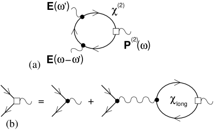
Figure 5: (a) Diagrammatic representation of the second-order susceptibility $\chi^{(2)}$ in terms of the effective electric field ${\bf E}$. ${\bf P}^{(2)}$ is the induced nonlinear polarization. The square vertex $\Box$ represents the factor $\varepsilon_{\mathrm{long}}^{-1}$ at the frequency of ${\bf P}^{(2)}$. It appears if one self-consistently takes into account the electric field due to the polarization $\mathbf{P}^{(2)}$ of the electron system and is given by the RPA series shown in Fig. (b). The wriggly line refers to the electron-electron interaction through the electromagnetic field and is absorbed into the matrix elements $\mathbf{D}$. Note, $\chi_{\mathrm{long}}$ only acts on the longitudinal field components, see text. The factor $\varepsilon_{\mathrm{long}}^{-1}$ can be enhanced by the plasma resonance.

The response theory clarifies how collective plasma excitations affect SFG. They essentially enter in two ways, both of which are controlled by the full (not only longitudinal) dielectric function $\varepsilon$:

First, the effective electric field is expressed in terms of the external field by means of Fresnel formulae SMD87 ; HBB94 ; Luce97 ; LuceLDA ; AtK02 , which contain contributions of order $1/\varepsilon$ for small $\varepsilon$. The dielectric function $\varepsilon$ becomes small if the frequency of the external field is close to the plasma frequency. This contribution can be interpreted as field enhancement. In addition, the outgoing (sum-frequency) electric field ${\bf E}_{\mathrm{out}}$ also contains terms that are enhanced for small $\varepsilon$ due to the Fresnel factors. This enhancement is most pronounced if the sum frequency is close to the plasma frequency.

Secondly, the longitudinal component of the nonlinear polarization ${\bf P}^{(2)}$ of the electron system is accompanied by an electric field ${\bf E}^{(2)}$ given by Eq. (13). Thus, the factor $\varepsilon_{\mathrm{long}}^{-1}$ appears in the nonlinear susceptibility in Eq. (14) and thus in $\mathbf{P}^{(2)}$ HB . This leads to an enhancement of the SFG light due to the longitudinal part of $\mathbf{P}^{(2)}$ if the sum frequency is close to the plasma frequency.

II.2 Two-photon photoemission

To demonstrate the similarities between SFG and 2PPE, we continue by summarizing the results of the response theory for 2PPE. We consider the same band structure as for SFG, which is characterized by single-electron energies $E_{{\bf k}_{\|}l}$. We emphasize that this band structure contains the bulk states with the $z$-component $k_{z}$ of ${\bf k}$ included in $l$.

The response theory starts from the observation that the photoelectron current $j(t;{\bf k},\sigma)$ of electrons of momentum ${\bf k}$ and spin $\sigma$ is given by the change of occupation of the vacuum state $|{\bf k}\sigma,{\mathrm{out}}\rangle$ outside of the crystal. However, in practice the time-dependence of $j$ is not measured, but only the total photoelectron yield ${\cal N}({\bf k},\sigma)=\int dt\>j(t;{\bf k},\sigma)$. This is similar to SFG, where only the time-integrated intensity is measured. The response theory directly determines the photoelectron yield ${\cal N}$. To prepare the discussion it is useful to first consider ordinary single-photon photoemission.

Single-photon photoemission: The photoelectron yield is given by

$${\cal N}({\bf k},\sigma)=\sum_{{\bf q}}\int dt_{1}\,dt_{2}\,\eta_{ij}({\bf q};t_{1},t_{2};{\bf k},\sigma)\,E_{i}({\bf q},t_{1})\,E_{j}(-{\bf q},t_{2}),$$ (15)

with the response function (see App. B)

$$\eta_{ij}({\bf q};t_{1},t_{2};{\bf k},\sigma)=\frac{e^{2}}{\hbar^{2}}\frac{\gamma_{{\bf k}\sigma,{\mathrm{out}};{\bf k}\sigma,{\mathrm{in}}}}{\Gamma_{{\bf k}\sigma,{\mathrm{in}};{\bf k}\sigma,{\mathrm{in}}}}\sum_{\lambda}D^{i}_{{\bf k}\sigma,{\mathrm{in}};{\bf k}_{\|}\lambda}(q_{z})$$ (16)

$$\quad{}\times\exp\!\left[i\frac{E_{{\bf k}_{\|}\lambda}-E_{{\bf k}\sigma,{\mathrm{in}}}}{\hbar}(t_{2}-t_{1})\right]e^{-\Gamma_{{\bf k}_{\|}\lambda;{\bf k}\sigma,{\mathrm{in}}}|t_{2}-t_{1}|}$$

$$\quad{}\times f(E_{{\bf k}_{\|}\lambda})\,D^{j}_{{\bf k}_{\|}\lambda;{\bf k}\sigma,{\mathrm{in}}}(-q_{z}).\qquad\qquad\qquad\quad\;\;\;$$

Here, $|{\bf k}\sigma,{\mathrm{in}}\rangle$ is a state with momentum ${\bf k}$ and spin $\sigma$ inside the crystal but above the vacuum energy. We have again neglected the momentum transferred by the photon. The standard diagrammatic representation of ordinary photoemission is shown in Fig. 6 Feder . The effective field ${\bf E}$ within the solid should again be expressed in terms of the external light field with the help of the proper boundary conditions. The response function $\eta$ will play a role when we discuss the various contributions to 2PPE.

Figure 6: Diagrammatic representation of the relation $\mathbf{j}\propto\int dt_{1}\,dt_{2}\,\eta_{ij}\,E_{i}E_{j}$ for the photoelectron current in ordinary photoemission Feder . The wavy lines denote the effective electric field ${\bf E}$ within the solid and the arrow denotes the emitted electron current ${\bf j}$ (or the photoelectron yield), which is of second order in the electric field. The response function $\eta$ is discussed in the text. The dots ($\bullet$) denote dipole matrix elements $\mathbf{D}$.

We briefly commend on the structure of this expression: The prefactor $\gamma_{{\bf k}\sigma,{\mathrm{out}};{\bf k}\sigma,{\mathrm{in}}}/\Gamma_{{\bf k}\sigma,{\mathrm{in}};{\bf k}\sigma,{\mathrm{in}}}$ describes the probability that electrons excited above the vacuum energy actually leave the crystal. Photoemission is often described by a three-step picture BS ; FFW ; WD : First, electrons are excited, then they are transported to the surface, and finally they leave the crystal. In this work we are mainly interested in the first step. The second and third steps are incorporated phenomenologically by effective relaxation rates $\Gamma_{{\bf k}\sigma,{\mathrm{in}};{\bf k}\sigma,{\mathrm{in}}}$, which describe electrons dropping below $E_{\mathrm{vac}}$ before they reach the surface, and effective transition rates $\gamma_{{\bf k}\sigma,{\mathrm{out}};{\bf k}\sigma,{\mathrm{in}}}$ from states above $E_{\mathrm{vac}}$ within the solid to free electron states outside of the solid. Note, the yield is proportional to the electric field squared and thus to the intensity of the incoming light.

Two-photon photoemission: The total 2PPE yield consists of the three contributions

$${\cal N}^{\mathrm{2PPE}}={\cal N}^{\mathrm{2PPE}}_{\mathrm{irr}}+{\cal N}^{\mathrm{2PPE}}_{\mathrm{red,1}}+{\cal N}^{\mathrm{2PPE}}_{\mathrm{red,2}}$$ (17)

corresponding to Fig. 7(a), (b), and (c), respectively. The second and third term arise from the nonlinear optical properties of the solid: Close to the surface the effective field ${\bf E}$ leads to a second-order polarization ${\bf P}^{(2)}$, see Eq. (5), which is accompanied by an electric field ${\bf E}^{(2)}$. This field may contribute to photoemission, leading to the processes in Fig. 7(b) and (c). The second-order field ${\bf E}^{(2)}$ is also responsible for SFG accompanying 2PPE. However, this SFG is usually a small effect since the SFG light intensity is of sixth order in dipole matrix elements $\mathbf{D}$, see Eqs. (7) and (10), whereas the 2PPE current is of fourth order, as is shown below in Eq. (24). This changes if the sum frequency is close to the plasma frequency, in which case SFG is enhanced as discussed at the end of Sec. II.1.

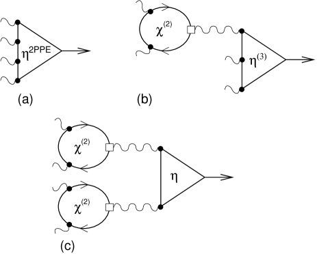
Figure 7: Diagrammatic representation of contributions to the 2PPE yield ${\cal N}^{\mathrm{2PPE}}$. (a) Direct irreducible contribution ${\cal N}^{\mathrm{2PPE}}_{\mathrm{irr}}$ involving four transitions induced by the effective electric field ${\bf E}$. (b) Reducible process involving conversion of two photons to a SFG photon and subsequent photoemission of third order in the fields, yielding ${\cal N}^{\mathrm{2PPE}}_{\mathrm{red,1}}$. (c) Reducible process involving conversion of all four photons to two SFG photons and ordinary photoemission (of second order in the fields) induced by the SFG light, yielding ${\cal N}^{\mathrm{2PPE}}_{\mathrm{red,2}}$. The dots ($\bullet$) denote dipole matrix elements $\mathbf{D}$. The square vertex ($\Box$), representing a factor of $\varepsilon_{\mathrm{long}}^{-1}$, is defined in Fig. 5(b). Plasma excitations again enter through this vertex.

Since the diagram in Fig. 7(a) cannot be cut into two by severing a single photon line, the first term ${\cal N}^{\mathrm{2PPE}}_{\mathrm{irr}}$ is irreducible, while the other two are reducible. The irreducible contribution in Eq. (17) can be written as

$${\cal N}^{\mathrm{2PPE}}_{\mathrm{irr}}=\int dt_{1}\,dt_{2}\,dt_{3}\,dt_{4}\;\eta^{\mathrm{2PPE}}_{ijkl}(t_{1},t_{2},t_{3},t_{4})\,E_{i}(t_{1})\,E_{j}(t_{2})\,E_{k}(t_{3})\,E_{l}(t_{4}),$$ (18)

which is of fourth order in the electric field and of second order in the incoming intensity. This is already clear from the simple picture in Fig. 2: The occupation of the intermediate state $|2\rangle$ is proportional to the light intensity. To reach state $|3\rangle$ above $E_{\mathrm{vac}}$ another absorption is required, leading to a total proportionality to the intensity squared.

Obviously, the structure of Eq. (18) is very similar to Eq. (7) for the SFG yield:

$${\cal I}^{(2)} \propto \int dt\,dt_{1}\,dt_{2}\,dt_{3}\,dt_{4}\;\chi^{(2)}_{ijk}(t-t_{1},t_{1}-t_{2})\,\chi^{(2)}_{ilm}(t-t_{3},t_{3}-t_{4})$$ (19)

$${}\times E_{j}(t_{1})\,E_{k}(t_{2})\,E_{l}(t_{3})\,E_{m}(t_{4}).$$

Hence, we expect similar interference effects in both cases.

The other two contributions to ${\cal N}^{\mathrm{2PPE}}$ are

$${\cal N}^{\mathrm{2PPE}}_{\mathrm{red,1}}=-4\pi\int dt_{1}\,dt_{2}\,dt_{3}\;\eta^{(3)}_{ijk}\>\Big{[}P_{i}^{(2)}(t_{1})\,E_{j}(t_{2})\,E_{k}(t_{3})$$ (20)

$$\;{}+E_{i}(t_{1})\,P_{j}^{(2)}(t_{2})\,E_{k}(t_{3})+E_{i}(t_{1})\,E_{j}(t_{2})\,P_{k}^{(2)}(t_{3})\Big{]},$$

and

$${\cal N}^{\mathrm{2PPE}}_{\mathrm{red,2}}=(4\pi)^{2}\int dt_{1}\,dt_{2}\;\eta_{ij}\>P_{i}^{(2)}(t_{1})\,P_{j}^{(2)}(t_{2}),$$ (21)

where $\eta$ is given in Eq. (16). Since the nonlinear susceptibility $\chi^{(2)}$ and hence $\mathbf{P}^{(2)}$ contains three dipole matrix elements, the reducible contributions to the photoelectron current are of higher order in dipole matrix elements and are thus usually small. However, the longitudinal component of ${\bf P}^{(2)}$ contains a factor $\varepsilon_{\mathrm{long}}^{-1}$. If the nonlinear polarization is enhanced due to a bulk plasma resonance at the sum frequency, one expects significant contributions from the reducible terms. The response functions $\eta^{(3)}$ and $\eta^{\mathrm{2PPE}}$ are given in App. B.

We next consider the response functions $\eta$, $\eta^{(3)}$, and $\eta^{\mathrm{2PPE}}$ which determine the yield ${\cal N}^{\mathrm{2PPE}}$. The functions $\eta^{(3)}$ and $\eta^{\mathrm{2PPE}}$ appearing in Eqs. (20) and (21), respectively, are of the same general form as $\eta$, Eq. (16), but have more terms resulting from different orders of the time arguments. We now first present the structure of the response expression for the main, irreducible contribution to the 2PPE yield, Eq. (18), and then discuss its physical interpretation. Fully written out, Eq. (18) reads

$${\cal N}_{\mathrm{irr}}^{\mathrm{2PPE}}({\bf k},\sigma) = \sum_{{\bf q}_{1}{\bf q}_{2}{\bf q}_{3}}\int dt_{1}\,dt_{2}\,dt_{3}\,dt_{4}\>\eta^{\mathrm{2PPE}}_{ijkl}({\bf q}_{1},{\bf q}_{2},{\bf q}_{3};t_{1},t_{2},t_{3},t_{4};{\bf k},\sigma)\,E_{i}({\bf q}_{1},t_{1})\,E_{j}({\bf q}_{2},t_{2})\,$$ (22)

$${}\times E_{k}({\bf q}_{3},t_{3})\,E_{l}(-{\bf q}-{\bf q}_{1}-{\bf q}_{2},t_{4}).$$

Defining the complex transition energy

$$\Omega_{{\bf k}_{\|}l;{\bf k}^{\prime}_{\|}l^{\prime}}\equiv\frac{E_{{\bf k}_{\|}l}-E_{{\bf k}^{\prime}_{\|}l^{\prime}}}{\hbar}-i\Gamma_{{\bf k}_{\|}l;{\bf k}^{\prime}_{\|}l^{\prime}},$$ (23)

we obtain the response function

$$\eta^{\mathrm{2PPE}}_{ijkl}({\bf q}_{1},{\bf q}_{2},{\bf q}_{3};t_{1},t_{2},t_{3},t_{4};{\bf k},\sigma)=\frac{e^{4}}{\hbar^{4}}\,\frac{\gamma_{{\bf k}\sigma,{\mathrm{out}};{\bf k}\sigma,{\mathrm{in}}}}{\Gamma_{{\bf k}\sigma,{\mathrm{in}};{\bf k}\sigma,{\mathrm{in}}}}\sum_{\lambda_{1}\lambda_{2}\lambda_{3}}D^{i}_{{\bf k}\sigma,{\mathrm{in}};{\bf k}_{\|}\lambda_{1}}(q_{1z})\,D^{j}_{{\bf k}_{\|}\lambda_{1};{\bf k}_{\|}\lambda_{2}}(q_{2z})\,$$ (24)

$$\;{}\times D^{k}_{{\bf k}_{\|}\lambda_{2};{\bf k}_{\|}\lambda_{3}}(q_{3z})\,D^{l}_{{\bf k}_{\|}\lambda_{3};{\bf k}\sigma,{\mathrm{in}}}(-q_{1z}-q_{2z}-q_{3z})$$

$$\;{}\times\bigg{\{}\Theta(t_{1}-t_{2})\,\Theta(t_{2}-t_{3})\,\Theta(t_{3}-t_{4})\,e^{-i\Omega_{{\bf k}_{\|}\lambda_{1};{\bf k}\sigma,{\mathrm{in}}}(t_{1}-t_{2})}\,e^{-i\Omega_{{\bf k}_{\|}\lambda_{2};{\bf k}\sigma,{\mathrm{in}}}(t_{2}-t_{3})}\,e^{-i\Omega_{{\bf k}_{\|}\lambda_{3};{\bf k}\sigma,{\mathrm{in}}}(t_{3}-t_{4})}\left[-f(E_{{\bf k}_{\|}\lambda_{3}})\right]{}$$

$$\quad{}-\Theta(t_{1}-t_{2})\,\Theta(t_{2}-t_{4})\,\Theta(t_{4}-t_{3})\,e^{-i\Omega_{{\bf k}_{\|}\lambda_{1};{\bf k}\sigma,{\mathrm{in}}}(t_{1}-t_{2})}\,e^{-i\Omega_{{\bf k}_{\|}\lambda_{2};{\bf k}\sigma,{\mathrm{in}}}(t_{2}-t_{4})}\,e^{-i\Omega_{{\bf k}_{\|}\lambda_{2};{\bf k}_{\|}\lambda_{3}}(t_{4}-t_{3})}\left[f(E_{{\bf k}_{\|}\lambda_{3}})\!-\!f(E_{{\bf k}_{\|}\lambda_{2}})\right]{}$$

$$\quad{}-\ldots\bigg{\}}.$$

There are eight terms in the curly braces, which correspond to different temporal orders of interactions with the electric field. Note, the dependence of 2PPE on light polarization is incorporated in the symmetries of the tensor $\eta^{\mathrm{2PPE}}_{ijkl}$, which depend on the dipole matrix elements $\mathbf{D}$. Unlike for the nonlinear optical response, these symmetries have not been discussed so far. It would be very interesting to determine the symmetries for surfaces of nonmagnetic and magnetic solids.

Figure 8: Interpretation of one of the processes contributing to 2PPE. An electron is excited from a pure state $|{\bf k}_{\|}\lambda_{2}\rangle$ in the Fermi sea to a pure state $|{\bf k}\sigma,{\mathrm{in}}\rangle$ above $E_{\mathrm{vac}}$ by four interactions with the electric field at the times $t_{i}$, as expressed by Eqs. (22) and (24). Note, the photoelectron current is proportional to the fourth power of the electric field and thus to the intensity squared, as expected for two-photon photoemission. The heavy wavy lines denote superpositions of states $|{\bf k}_{\|}\lambda_{2}\rangle$ and $|{\bf k}_{\|}\lambda_{3}\rangle$, $|{\bf k}_{\|}\lambda_{2}\rangle$ and $|{\bf k}\sigma,{\mathrm{in}}\rangle$ etc., while the black dots represent pure eigenstates. Compare with Fig. 4 for SFG.

Equation (24) forms the basis for our discussion of 2PPE. To clarify the time dependence exhibited in Eq. (24) we discuss the second term, the others are in principle similar but correspond to different orders of the times $t_{i}$. The processes described by this term are illustrated in Fig. 8. The system starts in equilibrium from the state $|{\bf k}_{\|}\lambda_{2}\rangle$. The first interaction with the electric field takes place at time $t_{3}$ and creates a superposition of the states $|{\bf k}_{\|}\lambda_{2}\rangle$ and $|{\bf k}_{\|}\lambda_{3}\rangle$, leading to oscillations at the frequency $(E_{{\bf k}_{\|}\lambda_{3}}-E_{{\bf k}_{\|}\lambda_{2}})/\hbar$ expressed by the third exponential factor in this term. The Fermi factors ensure that one of the states is initially occupied and that the other one is empty. Let us assume that $|{\bf k}_{\|}\lambda_{2}\rangle$ is occupied. The second interaction at $t_{4}$ changes the state into a superposition of $|{\bf k}_{\|}\lambda_{2}\rangle$ and the vacuum state $|{\bf k}\sigma,{\mathrm{in}}\rangle$, leading to oscillations at the corresponding difference frequency (second exponential factor), and the third interaction at $t_{2}$ creates a superposition of the vacuum state and $|{\bf k}_{\|}\lambda_{1}\rangle$. After the fourth interaction the electron is in a pure state above $E_{\mathrm{vac}}$ and can leave the solid with finite probability. Of course, due to the sum over bands there are usually several contributions of this type. Only if the superpositions decay very rapidly compared to the pure states, a description in terms of rate equations, as suggested by Fig. 2, is applicable Kno00 ; Rol1 ; Rol2 . Also compare the discussion of SFG above, see Fig. 4.

While SFG is only governed by the dephasing rates but not the energy relaxation rates, 2PPE depends on both. This is because in the 2PPE response function $\eta^{\mathrm{2PPE}}$ the change of occupation of states enters besides the polarization of the electron gas, whereas SFG only depends on the latter.

Note, the 2PPE yield contains four dipole matrix elements. Thus, even for inversion-symmetric crystals parity does not forbid 2PPE from the bulk. However, 2PPE is sensitive to a surface region of a thickness given by the mean free path of electrons above $E_{\mathrm{vac}}$. The optical penetration depth is typically significantly larger than the mean free path and thus does not enter here. Equations (16) and (24) also illustrate that 2PPE is sensitive to specific points in the Brillouin zone: The photoelectron momentum ${\bf k}$ measured by momentum-resolved 2PPE is approximately the same as the lattice momentum of the original unperturbed electron and also of the intermediate state due to the small photon momentum. These effects obviously require a theoretical description that considers the ${\bf k}$-dependent states in the solid, like our approach does as opposed to both the random-${\bf k}$ approximation and Bloch equations. In view of the importance of angle-resolved (ordinary) photoemission spectroscopy (ARPES) for, e.g., cuprate high-$T_{c}$ superconductors, ${\bf k}$-resolved 2PPE is expected to yield interesting results in the future. On the other hand, if one only measures the total number of photoelectrons, the ${\bf k}$-space resolution is lost and 2PPE and SFG give very similar information. It is obvious that 2PPE has the disadvantage of being limited to frequencies $\omega_{1}$, $\omega_{2}$ such that $E_{F}+\hbar\omega_{1}+\hbar\omega_{2}$ lies above the vacuum energy, unlike SFG. As stated already the SFG accompanying 2PPE is usually small since additional dipole matrix elements are involved.

The response expressions show that collective plasma excitations affect 2PPE in two ways: First, exactly like for SFG the effective field ${\bf E}$ within the metal differs from the external field due to linear screening and is enhanced close to the plasmon resonance. Secondly, the reducible contributions in Eqs. (20) and (21) depend on the second-order polarization ${\bf P}^{(2)}$, which contains a factor of $\varepsilon_{\mathrm{long}}^{-1}$, see Eq. (14). ${\bf P}^{(2)}$ is enhanced if the sum frequency is close to the plasma frequency. In 2PPE this enhancement enters only in the reducible contributions in Eqs. (20) and (21).

III Discussion

The aim of the present section is to discuss and illustrate the results of the response theory for time-resolved SFG and 2PPE. In particular, we consider time-dependent effects on the femtosecond time scale. Our results exhibit the intimate relation between SFG and 2PPE. We can already gain insight by studying the general structure of the response expressions for SFG and 2PPE, for example Eqs. (7) and (18), respectively, independently of the specific approximations made here. For clarity we apply our response theory to a simple model system.

III.1 Time-dependent effects in SFG and 2PPE

The response expressions of the preceding section are valid for any time dependence of the exciting laser field. The time enters the response expressions for both SFG and 2PPE in two ways, apart from the step functions from causality, cf. Eqs. (10), (16), and (24): The difference between the time arguments of electric fields appears in exponentials oscillating at the transition frequency of the involved electron states and in exponentials decaying with the dephasing rate of the superposition of the two states, and, for 2PPE, also exponentials decaying with the energy relaxation rate of an intermediate state. (See the discussion of Figs. 4 and 8 for the interpretation of SFG and 2PPE in terms of electronic excitations.) The time passing between absorptions can be controlled by the pulse shape of the exciting laser pulses: If the total duration $T$ of a pulse of arbitrary shape is much larger than typical relaxation times $\tau$ then the yield depends on the probability to absorb two photons within a time interval $\tau$, which is independent of $T$. On the other hand, for $T\ll\tau$ there is almost no relaxation during the pulse. Thus the response theory reproduces the well-known result that $\tau$ can only be inferred from SFG or 2PPE experiments if the total pulse duration is $T\sim\tau$.

To be more specific, in most experiments two approximately Gaussian pulses are used (pump-probe method) Ste92 ; HMKB97 ; Sim98 ; KSR98 ; Gud99 ; Schoe ; Aesch1 ; Aesch2 ; Wolf1 ; Hoef97 ; Cao97 ; Petek ; Wolf2 ; Leh99 ; Kno00 ; GWH00 ; SBW02 ; ONP02 ; Gerb ; Ae.cluster . If the two pulses are of different mean frequencies $\omega_{1}$ and $\omega_{2}$ (two-color case) and one measures the SFG or 2PPE response at the sum frequency $\omega_{1}+\omega_{2}$ then it is obvious which photon was absorbed out of which pulse. Then for long time delay $\Delta T$ compared to the single-pulse duration the relaxation rate of intermediate states can be read of directly from the $\Delta T$ dependence of the total yield. In pump-probe experiments with two pulses of the same mean frequency $\omega$ (single-color case), photons can be absorbed out of the same or different pulses. However, the contribution with all absorptions out of the same pulse obviously does not depend on $\Delta T$, just leading to a constant background. Note, in all these cases only a typical relaxation time enters, which usually is a weighted average over relaxation times of many states Weida . If only a single relevant intermediate state is present, e.g., for a quantum-well state, or if there are many but of similar relaxation rate, the relaxation time extracted from experiment will be the actual dephasing time of intermediate states. However, if intermediate states with very different dynamical properties are involved, for example if both sp and d bands are relevant, the measured relaxation time does not describe any single excited electron state.

In pump-probe SHG Ste92 ; HMKB97 ; Sim98 ; KSR98 ; Gud99 or pump-probe single-color 2PPE Aesch2 ; Cao97 ; Petek ; Wolf2 ; Kno00 experiments, time-dependent interference effects are especially pronounced. Their origin is the following: The first absorption of a photon of frequency $\omega$ sets up an oscillating polarization of the excited electrons. Now the probability of a second absorption depends on the relative phase of the oscillating polarization and the second photon. Since the oscillating polarization is described by the off-diagonal components of the density matrix $\rho$, a description in terms of rate equations, which omits these components, is unable to describe interference.

For further illustration of this interference, we show results for SHG and 2PPE for a simple model. Unless stated otherwise, this model consists of three bands. The lowest one is a three-dimensional tight-binding band $1$ with band center at rem.param $-3.33\>{\rm eV}$ (all energies are measured relative to the Fermi energy) and half width $3.81\>{\rm eV}$. The band maximum is at ${\bf k}=0$. The second, rather flat tight-binding band $2$ is centered at $2.29\>{\rm eV}$ with half width $0.48\>{\rm eV}$ and maximum also at ${\bf k}=0$. Finally, there is a free electron band $3$ representing electrons above the vacuum energy $E_{\mathrm{vac}}=4.29\>{\rm eV}$. There exist points in the Brillouin zone for which the energy differences between bands 2 and 1 as well as between bands 3 and 2 both equal the photon energy of $\hbar\omega=3.05\>{\rm eV}$. We assume that the relaxation rates $\Gamma_{n_{1}n_{2}}$ only depend on the band indices $n_{1}$, $n_{2}$ but not on the ${\bf k}$ vector (see below). We use the energy relaxation rates $\hbar\Gamma_{22}=0.191\>{\rm eV}$ (corresponding to the lifetime $\tau_{2}=3.5\>{\rm fs}$) and $\hbar\Gamma_{33}=0.381\>{\rm eV}$ ($\tau_{3}=1.7\>{\rm fs}$) and no additional dephasing, i.e., $\Gamma_{n_{1},n_{2}}^{\mathrm{ph}}=0$ in Eq. (4). These short lifetimes are assumed to bring out the time-dependent effects more clearly. The dipole matrix elements are treated as constants.

In the following we use this model to show how time-dependent effects emerge from our response theory. For clarity we neglect the Fresnel formulae, which do not change the results qualitatively. We demonstrate that our theory gives reasonable results for a moderately complicated system. Obviously, it can be applied to a more realistic band structure at the expense of computation time. The boundary conditions (Fresnel factors) are also omitted for simplicity.

Figure 9: (a) Total yield of photoelectrons of momentum ${\bf k}$ for single-color pump-probe 2PPE as a function of the delay time $\Delta T$ between pump and probe pulses. The parameters of the model are given in the text. The ${\bf k}$ vector is chosen such that the transition frequencies perfectly match the frequency of incoming light. Only results for $\Delta T>0$ are shown, since the curve is symmetric about $\Delta T=0$ for identical pump and probe pulses. All curves in this and the following figures are scaled such that the limit for large $\Delta T$ is unity. (b) Total SHG yield for single-color pump-probe SHG as a function of the delay time $\Delta T$ using the same parameters. The inset shows the SHG yield for flat bands with transition frequencies that match the light frequency perfectly. Note, for extracting relaxation rates from experimental data the resolution of the photoelectron and SHG light detectors must be taken into account Weida .

In Fig. 9(a) we show the 2PPE photoelectron yield for a particular momentum ${\bf k}$ as a function of the delay time $\Delta T$ between two identical Gaussian pump and probe pulses. A mean photon energy of $\hbar\omega=3.05\>{\rm eV}$ is assumed, corresponding to a wave length of about $\lambda=400\>{\rm nm}$, and the duration of each pulse is $10.3\>{\rm fs}$ (full width at half maximum of the Gaussian envelope of the electric field). The vector ${\bf k}$ is chosen so that the transition energies between the bands match $\hbar\omega$. In Fig. 9(b) we show the total SHG photon yield for exactly the same system. Unlike 2PPE, SHG integrates over the whole Brillouin zone. Nevertheless, the overall similarity of Figs. 9(a) and (b) demonstrates the similarity of the response expressions for SHG and 2PPE, compare Eqs. (7) and (18), for example. It means that similar information, e.g., about the relaxation rates, can be obtained from both. The SHG curve is quite similar to the case of flat bands, shown in the inset in Fig. 9(b). This means that only a small region of ${\bf k}$ space contributes. The resulting interference between different ${\bf k}$ points becomes apparent in the tail of the interference pattern, where the main plot in Fig. 9(b) is more irregular and decays faster. This is the averaging effect discussed in Ref. Weida . More precisely it is an interference effect between different oscillation frequencies of superpositions of different states.

The 2PPE and SHG interference patterns in Fig. 9 show the well-known $8:1$ enhancement of the signal for $\Delta T=0$. This enhancement is due to the yield being of fourth order in the field: For a single pulse the signal would be proportional to $E^{4}$, for two isolated pulses this becomes $2E^{4}$, but for two overlapping pulses the amplitude is doubled, leading to $(2E)^{4}=16E^{4}$.

For both SHG and 2PPE, the central part of the interference pattern, which corresponds to short delay times $\Delta T$ up to about the single-pulse duration $T$, is dominated by the four-field autocorrelation function

$${\cal A}_{ijkl}^{(4){}}(\Delta T)\equiv\int d\omega_{1}\,d\omega_{2}\,d\omega_{3}\;E_{i}(\omega_{1})\,E_{j}(\omega_{2})\,E_{k}(\omega_{3})E_{l}(-\omega_{1}-\omega_{2}-\omega_{3}).$$ (25)

This central part stems from the overlap of the two pulses and would be present even for very fast relaxation: Then the response functions $\chi^{(2)}$ and $\eta^{\mathrm{2PPE}}$ are very sharply peaked in time and thus nearly constant in frequency space, leading to ${\cal I}^{(2)}\propto{\cal A}^{(4){}}$ and ${\cal N}^{\mathrm{2PPE}}_{\mathrm{irr}}\propto{\cal A}^{(4){}}$ for the SHG and 2PPE yield, respectively, see Eqs. (7) and (18). The autocorrelation signal alone is shown in Fig. 10(b).

Figure 10: Demonstration of the lifetime dependence of 2PPE. (a) Total 2PPE yield for the same model parameters as used in Fig. 9 with a lifetime of states in the intermediate band of $\tau_{2}=6.9\>{\rm fs}$ (dotted curve) and with the very small value $\tau_{2}=0.86\>{\rm fs}$ (heavy solid curve). The dashed curves show the exponential decay with the dephasing rate $\Gamma_{12}=\tau_{2}^{-1}/2$ for $\tau_{2}=6.9\>{\rm fs}$. (b) Four-field autocorrelation function of the pump-probe laser field. Note the similarity to the fast-relaxation result in Fig. (a). The black bar denotes half the laser pulse duration.

In Sec. II we have discussed the response expressions for time-dependent SFG and 2PPE, (10) and (24), respectively. The first interaction creates an oscillating polarization. There is interference if the phase information is still preserved when the second photon is absorbed. This is governed by the dephasing time $\Gamma_{21}$. Thus the interference effects should decay with the time constant $\Gamma_{21}^{-1}$ for large delays $\Delta T$. This is shown in Fig. 10(a) for moderately fast ($\tau_{2}=6.9\>{\rm fs}$) and extremely fast ($\tau_{2}=0.86\>{\rm fs}$) relaxation. For the slower relaxation the tail indeed decays with $\Gamma_{21}^{-1}$ but to observe this one obviously has to look at rather large $\Delta T$ where the interference is already weak. For fast relaxation the curve is nearly indistinguishable from the autocorrelation in Fig. 10(b).

Figure 11: Demonstration of the dependence of 2PPE on the detuning of the intermediate band. The heavy solid curve shows the total 2PPE yield for the same parameters as used in Fig. 9 but with the intermediate band shifted downward in energy by $0.1\,\hbar\omega$. $\omega$ is the mean frequency of the exciting laser field. For comparison, the dotted curve shows the 2PPE yield for unshifted bands with matching transition frequencies. Note the beats apparent for $\Delta T\gtrsim 10\>\mathrm{fs}$. This shows how detuning affects the decay of the signal and needs to be taken into account when extracting relaxation rates from experiments.

However, there is another crucial origin of the decay of interference: Intermediate states with energies that do not exactly match the energy of the original state plus the photon energy lead to beats at the frequency of the detuning. This effect can be seen from the response expressions. We now discuss this for the case of SFG: For pulses of short duration $T$, the times $t_{1}$ and $t_{2}$ in Eq. (10) can be approximated by the pulse centers if we are interested in phenomena at frequencies small compared to $T^{-1}$. Then Eq. (10) shows that the polarization of the electron system shortly before the second interaction at $t_{1}$ is proportional to

$$\exp\!\left[i\frac{E_{{\bf k}_{\|}l}-E_{{\bf k}_{\|}l^{\prime}}}{\hbar}\,(t_{1}-t_{2})\right]e^{-\Gamma_{{\bf k}_{\|}l^{\prime};{\bf k}_{\|}l}(t_{1}-t_{2})}e^{-i\omega t_{2}},$$ (26)

omitting the sum over states. The last factor stems from the electric field of frequency $\omega$ describing the first interaction at time $t_{2}<t_{1}$. The decaying exponential obviously describes the decay of interference with the dephasing rate $\Gamma_{{\bf k}_{\|}l^{\prime};{\bf k}_{\|}l}$. The oscillating terms are of the form $\exp[-i\delta\omega(t_{1}-t_{2})]\,\exp(-i\omega t_{1})$ with $\delta\omega=(E_{{\bf k}_{\|}l^{\prime}}-E_{{\bf k}_{\|}l})/\hbar\;-\;\omega$. Thus we expect slow beats with the detuning frequency $\delta\omega$, which lead to an initial decay of the signal on a time scale of $(\delta\omega)^{-1}$. There should be a recurring signal at large delay times, but this is in practice suppressed by relaxation. A similar argument can be made for 2PPE using Eq. (24). The effect is clearly seen in Fig. 11 for 2PPE: The width of the pattern is reduced by the detuning. Its tails also become more irregular.

Next, we turn to the effect of the band structure. We first discuss SHG. The SHG yield is determined by a sum over many transitions of different energies and dephasing rates, see Eq. (10). If the decay is governed by dephasing one observes the smallest dephasing rate at large time delays $\Delta T$. However, at intermediate $\Delta T$ one sees an averaged rate. The dephasing rate $\Gamma_{{\bf k}_{\|}l;{\bf k}_{\|}l^{\prime}}$ for two bands $l$ and $l^{\prime}$ should usually not change dramatically with ${\bf k}$. On the other hand, the contribution of detuning is necessarily different for transitions with different transition frequencies. Thus, in the interference pattern a continuum of beating frequencies appears. Consequently, the initial decay is governed by an average detuning and later, probably unobservable, recurring signals are strongly reduced by destructive interference of different beating frequencies. The averages are weighted by a factor approximately inversely proportional to the detuning, as seen from Eq. (11). For narrow valence and intermediate state bands the average is restricted to a small effective band width $W$. For broader bands but constant relaxation rates throughout each band the dependence of numerical results (not shown) for the SHG yield on the width of the intermediate band turns out to be weak, since in this case all contributing processes are governed by the same relaxation rates rem.SHGband . Hence, if only a single intermediate state or a few states contribute significantly Luce96 or if there is a narrow band with uniform relaxation rates, the Bloch equations should work well. In this case our expressions reduce to a perturbative solution of the Bloch equations.

On the other hand, if there is strong electron-electron scattering at certain ${\bf k}$ vectors, e.g., due to Fermi surface nesting, the rates can be strongly ${\bf k}$ dependent. If many states of different relaxation rates enter the SHG photon yield, then for broad bands the description of SHG using optical Bloch equations with a single intermediate state is not justified. If interference patterns are fitted with results from Bloch equations, there is no simple relation between the extracted relaxation rate and the dephasing rates of the excited electrons.

For 2PPE the situation is quite different, since this method allows to probe specific momenta ${\bf k}$ in the Brillouin zone. Here, the band width is not crucial. There are typically several contributions to the photoelectron yield, since there are several unoccupied bands. The contributions are again weighted with the inverse detuning, but now there is only a small number of states involved for fixed photoelectron momentum ${\bf k}$. Thus a description in terms of a small number of states, e.g., by optical Bloch equations, is valid. However, if one experimentally integrates over ${\bf k}$, 2PPE behaves much like SFG.

As mentioned above, 2PPE is generally accompanied by SFG, although the latter is generally smaller in intensity due to the appearance of additional dipole matrix elements. It might be interesting to perform both SFG and 2PPE experiments on the same sample. The two techniques are complementary in that 2PPE gives information about specific points in the Brillouin zone whereas SFG averages over the whole zone. Furthermore, comparison of Eqs. (10) and (24) shows that while the general form of the expressions for SFG and 2PPE is similar, they do depend on the material parameters in quite different ways. We give three examples: First, 2PPE also depends on the energy relaxation rates (lifetimes) directly, whereas SFG only depends on the dephasing rates. Secondly, SFG crucially depends on the dipole matrix element ${\bf D}_{31}$ of the transition from the excited state above $E_{\mathrm{vac}}$ to the original state in the Fermi sea, whereas 2PPE does not. Thus comparison of SFG and 2PPE may proof useful for measuring the dipole matrix elements. Thirdly, SFG generally results from a much thinner surface region than 2PPE and the relaxation rates obtained from 2PPE are more bulk-like, allowing to study the dependence of the rates on the distance from the surface. Finally, we have shown that there is a contribution to 2PPE from SFG light generated within the solid, see Eqs. (20) and (21) as well as Figs. 7(b) and (c). Simultaneous measurement of SFG and 2PPE may allow to detect this interesting effect.

III.2 Collective plasma excitations

Since SFG and 2PPE may be strongly enhanced by collective plasma excitations, it is useful to discuss them in the framework of the response theory. Our goal is to show plasmon enhancement of SFG and 2PPE in principle, even though the plasma frequency is larger than currently accessible laser frequencies in some metals (but not, for example, in silver, many heavy-fermion metals, and the interesting compound $\mathrm{MgB}_{2}$). Note, the plasma frequency is smaller in clusters, for which the same general picture applies.

We have seen in Sec. II that in both SFG and 2PPE field enhancement of the effective electric field ${\bf E}$ is described by the Fresnel formulae SMD87 ; HBB94 ; Luce97 ; LuceLDA ; AtK02 . This mechanism is relevant at the frequency of the exciting laser field and, in the case of SFG, also at the sum frequency for the outgoing SFG light. It corresponds to the coupling of the external light field to plasmon-polaritons in the solid Board .

The second important origin of plasmon enhancement is the screening of the nonlinear polarization ${\bf P}^{(2)}$, which is caused by the effective electric field ${\bf E}^{(2)}$ accompanying the longitudinal part of $\mathbf{P}^{(2)}$ and appears at the sum frequency. Since the electric field $\mathbf{E}^{(2)}$ is longitudinal, a true plasmon excitation is involved. It is important to remember that the exciting light does couple to plasmons in real solids; this coupling is only absent in simple jellium models Barton ; Board .

Note, in the case of pump-probe SFG with two pulses of different mean frequencies $\omega_{1}$ and $\omega_{2}$, one of them and the sum frequency $\omega_{1}+\omega_{2}$ can be close to the plasma frequency. This so-called double resonance leads to a particularly strong enhancement Lie99 . Surface plasmons lie outside the scope of this paper, since they require a more detailed description of the surface. See Ref. Board for a discussion.

Motivated by 2PPE experiments on clusters Gerb , we briefly consider the plasmon decay. A plasmon decays into a single particle-hole pair BVV00 . The probability of this decay is determined by the phase space available for the final electron-hole pair. It is only energetically possible if the plasmon dispersion lies within the electron-hole continuum at the plasmon momentum ${\bf q}$, leading to Landau damping. On the other hand, decay into a single electron-hole pair may be possible close to the surface, since translational symmetry is broken and $q_{z}$ is not conserved. If the energy of the electron is higher than the vacuum energy, photoemission may result. Creation of several pairs is possible by subsequent inelastic electron-electron scattering. A plasmon also looses energy through inelastic scattering of the virtual electrons and holes in the loop in Fig. 5(b). This process is governed by the single-particle relaxation rates. The plasmon lifetime is thus shorter than typical lifetimes of the relevant excited electrons.

A plasma mode can be multiply excited. In a recent 2PPE experiment a doubly excited plasma mode of silver nanoparticles decays into a single electron-hole pair Gerb ; rem.clusters . What is actually observed is an enhancement of the 2PPE yield when the sum frequency is close to twice the plasma frequency. The origin of this effect is that 2PPE with the incident-light frequency close to the plasma frequency is enhanced due to field enhancement. The general process is not specific to clusters but is also relevant for flat surfaces. It would be interesting to look for this effect experimentally.

III.3 Further remarks

Concerning the range of validity of the second-order response theory we remark the following. We consider first pump-probe SFG with a very long delay time $\Delta T$. The first-order density operator $\rho^{(1)}$ describes the result of the first interaction. It contains a finite polarization (off-diagonal components) but no change of occupation (diagonal components), see Eq. (38). A change of occupation is only obtained from $\rho^{(2)}$ and higher-order contributions, which involve a larger number of dipole matrix elements and are usually small compared to $\rho^{(1)}$. However, the off-diagonal components usually decay faster than the diagonal ones so that for long delay times the higher-order change of occupation can dominate over the second-order polarization and the second-order approximation breaks down. On the other hand, our expressions for 2PPE already include the change of occupation due to the first pulse, since we have directly calculated the photoelectron yield to fourth order. Thus the results should hold even for long delay times. For the case that the polarization has decayed at the time of the second pulse, but the non-equilibrium occupation has not, the resulting limiting form of $\eta^{\mathrm{2PPE}}$ is given by Eq. (72). It only depends on the energy relaxation rates. This is the case where rate equations are appropriate Kno00 ; Rol1 ; Rol2 . Due to the vanishing polarization there are no interference effects.

There is an alternative and physically appealing description of pump-probe SFG and 2PPE as a two-step process: The first pulse creates a non-equilibrium distribution, which is probed by the second one. We now discuss the validity of calculations based on this picture. In App. A we derive an expression for the linear susceptibility of an electron gas in an arbitrary non-equilibrium state described by the density matrix $\rho_{\mathrm{neq}}$, see Eq. (45). If we insert $\rho^{(1)}$ due to the first pulse for $\rho_{\mathrm{neq}}$, we obtain a two-step description for $\chi^{(2)}$ and the polarization ${\bf P}^{(2)}$. Omitting the details, we only state that the result is identical to the one obtained directly for the second-order polarization ${\bf P}^{(2)}$, Eq. (5), but with the full susceptibility $\chi^{(2)}$ replaced by its irreducible part $\chi^{(2)}_{\mathrm{irr}}$ of Eq. (10). Thus, by assuming two separate interaction processes and treating each in a first-order approximation, we loose the screening of the second-order polarization. This is not justified if the sum frequency lies close to the plasma resonance.

Next we consider a two-step description of 2PPE: The 2PPE photoelectron yield ${\cal N}^{\mathrm{2PPE}}$ is expressed in terms of an arbitrary non-equilibrium density matrix $\rho_{\mathrm{neq}}$ as discussed in App. B. Then the second-order density matrix $\rho^{(2)}$ due to the first pulse is inserted for $\rho_{\mathrm{neq}}$. We reobtain the full irreducible fourth-order result ${\cal N}^{\mathrm{2PPE}}_{\mathrm{irr}}$ of Fig. 7(a), but only part of the reducible contributions, Fig. 7(b), (c): The two-step description neglects contributions of two photons out of different pulses being converted into one SHG photon. These contributions may become important if the sum frequency is close to a plasma resonance. In conclusion, the two-step picture of SFG and 2PPE is valid unless the response at the sum frequency is enhanced by plasmon effects.

Finally, we emphasize that our theory can also describe time-resolved SFG and 2PPE from ferromagnetically ordered systems. Ultimately, the light couples to the (spin) magnetization through spin-orbit coupling, which is incorporated, in principle, in the dipole matrix elements ${\bf D}$ and the band structure. The spin-dependent matrix elements can be calculated by a perturbative expansion in the spin-orbit coupling HB ; NOLI . SFG and 2PPE also depend on magnetic order through the band energies $E_{{\bf k}_{\|}l}$ and relaxation rates $\Gamma_{{\bf k}_{\|}l;{\bf k}_{\|}^{\prime}l^{\prime}}$, since $l$ also contains a spin index $\sigma$. Of particular importance for magnetically-ordered materials is the rotation of the polarization of SHG light relative to incident light (NOLIMOKE) HB ; NOLI ; Luce96 . As mentioned above, the light polarization is controlled by the symmetries of the tensor $\chi^{(2)}_{ijk}$, which are known for low-index surfaces Pan .

Compared to NOLIMOKE, 2PPE for magnetic systems has the advantage that in principle one can obtain information on the spin-dependent lifetimes of electrons in specific states $|{\bf k}_{\|}l\rangle$. The dependence of 2PPE on the light polarization for magnetic systems has not been studied so far. In the response theory this dependence is controlled by the symmetries of the tensor $\eta^{\mathrm{2PPE}}_{ijkl}$, as mentioned in Sec. II.2.

For pump-probe experiments with long time delay $\Delta T$ the main contribution to 2PPE comes from the change of occupation brought about by the pump pulse. Only in this case the photoelectron yield is proportional to the occupation of the corresponding intermediate states. If in addition the matrix elements and the relaxation rates out of vacuum states depend only weakly on spin, then Eq. (60) shows that the 2PPE yield becomes proportional to the spin-dependent occupation of these intermediate states:

$${\cal N}^{\mathrm{2PPE}}(\Delta T;{\bf k},\sigma)\propto\rho_{\mathrm{neq};{\bf k}\nu\sigma;{\bf k}\nu\sigma}(\Delta T)=n_{\mathrm{neq};{\bf k}\nu\sigma}(\Delta T),$$ (27)

where $n_{\mathrm{neq};{\bf k}\nu\sigma}$ denotes the non-equilibrium occupation of the state $|{\bf k}\nu\sigma\rangle$ after the pump pulse. Then the difference of the spin-up and spin-down 2PPE yield, ${\cal N}^{\mathrm{2PPE}}(\Delta T;{\bf k},\uparrow)-{\cal N}^{\mathrm{2PPE}}(\Delta T;{\bf k},\downarrow)$, is proportional to the difference of the occupations and thus to the transient magnetization of the intermediate states.

Note, circularly polarized light might excite electrons spin-selectively due to angular-momentum conservation. In our response theory these selection rules are incorporated in the dipole matrix elements $\mathbf{D}$. Conversely, spin-selective excitation will lead to corresponding polarization of the SFG light. The use of circularly polarized light in 2PPE and SFG is of particular interest regarding ferromagnets and transient magnetizations.

III.4 Conclusions

To summarize, we have presented a unified perturbative response theory for time-resolved SFG and 2PPE. The theory is fully quantum-mechanical and contains the interference effects described by off-diagonal components of the density matrix. It does not rely on any assumption about the time or frequency dependence of the exciting laser pulses. The solid is described by its band structure, relaxation rates, and dipole matrix elements. We have discussed metals but the response theory can be applied to semiconductors and insulators as well, see, e.g., Ref. ShA03 . Since the theory is formulated directly in the time domain, it presents a suitable framework for the discussion of the time-dependent physics of SFG and 2PPE. We have shown that similar information as from 2PPE can be gained from SHG. Of course, 2PPE is sensitive to specific momenta ${\bf k}$ in the Brillouin zone, while SHG in general is not. A simple tight-binding model of a metal has been studied in order to show that the theory gives reasonable numerical results and to illustrate the following effects important for the understanding of SFG and 2PPE.

We have shown how relaxation rates and detuning affect the interference patterns in single-color pump-probe SHG and 2PPE experiments: The lifetime in the intermediate states and their detuning with respect to the photon energy lead to a similar narrowing of the interference patterns. The effect of detuning must be taken into account in order to extract meaningful life times from such experiments. Also, in particular in SHG the measured relaxation rate is a weighted average over the relaxation rates of many excited states. Furthermore, the weights in this average change with the pump-probe delay. Thus different rates govern the decay of the interference pattern depending on the pump-probe delay—the decay is not simply exponential. We have also discussed the range of validity of the optical Bloch equations, applicable if only a few states contribute, and of semiclassical rate equations valid for very long pump-probe delays. Both approaches are limiting cases of our theory.

Finally, we have considered the role played by collective plasma excitations. Plasmon effects in both SFG and 2PPE can only partly be understood in terms of field enhancement at the surface. One also has to take the electric field accompanying a nonlinear polarization of the electron system into account. This effect leads to interesting additional contributions to 2PPE, in which incoming photons are converted into sum-frequency photons which then lead to ordinary photoemission. These contributions should be observable if the sum frequency is close to the plasma frequency.

Appendix A Response theory for the nonlinear optical response

In this appendix we derive the transverse second-order susceptibility and polarization for arbitrary pulse shapes of the exciting laser field. The resulting expressions allow to calculate the SFG yield for arbitrary pulse shapes, thereby going beyond the results of Hübner and Bennemann HB for continuous-wave, monochromatic light. The self-consistent-field approach EC is applied to a solid described by its band structure and relaxation rates. The flat surface is assumed to lie at $z=0$ with the solid at $z<0$. We neglect the intraband contribution, which is reasonable for optical frequencies.

The single-particle Hamiltonian is $H=H_{0}+V$, where $H_{0}$ describes the unperturbed solid with the normalized eigenstates $|{\bf k}_{\|}l\rangle$ and eigenenergies $E_{{\bf k}_{\|}l}$. ${\bf k}_{\|}$ is the crystal momentum parallel to the surface and all other quantum numbers, discrete as well as continuous, are collectively denoted by $l$ (see the discussion at the beginning of Sec. II.1).

The time-dependent perturbation is Schiff

$$V({\bf r},t)=-\frac{ie\hbar}{mc}\,{\bf A}({\bf r},t)\cdot{\mbox{\boldmath$\nabla$}}-\frac{ie\hbar}{2mc}\,[{\mbox{\boldmath$\nabla$}}\cdot{\bf A}({\bf r},t)]$$ (28)

with the vector potential ${\bf A}$, which is treated classically. We have made the usual approximation to neglect the quadratic term in ${\bf A}$ and have used a gauge with vanishing scalar potential. We will later need the temporal Fourier transform (using the convention of Ref. HB )

$$V({\bf r},\omega) = \int\frac{dt}{2\pi}\,e^{-i\omega t}\,V({\bf r},t)$$ (29)

$$= \frac{e\hbar}{m\omega}\,{\bf E}({\bf r},\omega)\cdot{\mbox{\boldmath$\nabla$}}+\frac{e\hbar}{2m\omega}\,[{\mbox{\boldmath$\nabla$}}\cdot{\bf E}({\bf r},\omega)],$$

where we have used ${\bf E}=-(1/c)\,\partial{\bf A}/\partial t$. Inserting the spatial Fourier transform we get

$$V({\bf r},\omega)=\frac{e\hbar}{m\omega}\sum_{\bf q}e^{-i{\bf q}\cdot{\bf r}}\,{\bf E}({\bf q},\omega)\cdot\left({\mbox{\boldmath$\nabla$}}-\frac{i{\bf q}}{2}\right).$$ (30)

The matrix elements of $V$ are

$$\langle{\bf k}_{\|}l|V|{\bf k}_{\|}+{\bf q}_{\|},l^{\prime}\rangle = \frac{e\hbar}{m\omega}\sum_{q_{z}}{\bf E}({\bf q},\omega)\cdot\langle{\bf k}_{\|}l|e^{-i{\bf q}\cdot{\bf r}}\left({\mbox{\boldmath$\nabla$}}-i{\bf q}/2\right)|{\bf k}_{\|}+{\bf q}_{\|},l^{\prime}\rangle$$ (31)

$$\equiv e\sum_{q_{z}}{\bf E}({\bf q},\omega)\cdot{\bf D}_{{\bf k}_{\|}l;{\bf k}_{\|}+{\bf q}_{\|},l^{\prime}}(q_{z},\omega)$$

using momentum conservation and ${\bf q}=({\bf q}_{\|},q_{z})$. Here,

$${\bf D}_{{\bf k}_{\|}l;{\bf k}_{\|}+{\bf q}_{\|},l^{\prime}}(q_{z},\omega)=\frac{\hbar}{m\omega}\,\langle{\bf k}_{\|}l|e^{-i{\bf q}\cdot{\bf r}}\left({\mbox{\boldmath$\nabla$}}-i{\bf q}/2\right)|{\bf k}_{\|}+{\bf q}_{\|},l^{\prime}\rangle.$$ (32)

If the field $\mathbf{E}$ were purely transverse the term $i{\bf q}/2$ in the parentheses would drop out, but this is not guaranteed close to a surface. It is not our goal to calculate ${\bf D}$ explicitly. We only remark that if one uses the dipole approximation HK90 ; HBB94 ; Luce97 ; LuceLDA ; NOLI ; Luce96 ; Luce98 ; AnH02 ; Shala $e^{-i{\bf q}\cdot{\bf r}}\cong 1$, the contribution from $i{\bf q}/2$ vanishes since we neglect the intraband contributions so that $l^{\prime}\neq l$, and the remainder gives Klings ; Voon

$$\frac{\hbar}{m\omega}\,\langle{\bf k}_{\|}l|{\mbox{\boldmath$\nabla$}}|{\bf k}_{\|}+{\bf q}_{\|},l^{\prime}\rangle=-\frac{1}{\hbar\omega}\,\langle{\bf k}_{\|}l|[H,{\bf r}]|{\bf k}_{\|}+{\bf q}_{\|},l^{\prime}\rangle$$ (33)

$$=-\frac{E_{{\bf k}_{\|}l}-E_{{\bf k}_{\|}+{\bf q}_{\|},l^{\prime}}}{\hbar\omega}\,\langle{\bf k}_{\|}l|{\bf r}|{\bf k}_{\|}+{\bf q}_{\|},l^{\prime}\rangle.$$

Since the response is dominated by contributions with $\hbar\omega\sim E_{{\bf k}_{\|}+{\bf q}_{\|},l^{\prime}}-E_{{\bf k}_{\|}l}$ the prefactor can be further approximated by unity if the frequency spectrum of the incoming light is sufficiently narrow. The dipole approximation should be justified since the electric field changes slowly on the scale of the lattice constant (the skin depth is about one order of magnitude larger than the lattice constant). However, our response theory for SFG does not require the dipole approximation to be made.

The time evolution of the density operator $\rho$ is described by the master or von Neumann equation Louisell ; Loudon

$$\frac{d}{dt}\rho=\frac{1}{i\hbar}\,[H,\rho]+{\cal R}[\rho].$$ (34)

The functional ${\cal R}[\rho]$ represents relaxation terms made explicit below. Matrix elements of $\rho$ are written as $\rho_{{\bf k}_{\|}l;{\bf k}^{\prime}_{\|}l^{\prime}}\equiv\langle{\bf k}_{\|}l|\rho|{\bf k}^{\prime}_{\|}l^{\prime}\rangle$. The master equation then reads Loudon

$$\frac{d}{dt}\rho_{{\bf k}_{\|}l;{\bf k}^{\prime}_{\|}l^{\prime}}=\frac{1}{i\hbar}\langle{\bf k}_{\|}l|[H_{0}+V,\rho]|{\bf k}^{\prime}_{\|}l^{\prime}\rangle+\delta_{{\bf k}_{\|}{\bf k}^{\prime}_{\|}}\delta_{ll^{\prime}}$$ (35)

$$\quad\times{\sum_{{\bf k}^{\prime\prime}_{\|}l^{\prime\prime}}}^{\prime}\gamma_{{\bf k}_{\|}l;{\bf k}^{\prime\prime}_{\|}l^{\prime\prime}}\rho_{{\bf k}^{\prime\prime}_{\|}l^{\prime\prime};{\bf k}^{\prime\prime}_{\|}l^{\prime\prime}}-\Gamma_{{\bf k}_{\|}l;{\bf k}^{\prime}_{\|}l^{\prime}}\rho_{{\bf k}_{\|}l;{\bf k}^{\prime}_{\|}l^{\prime}}.$$

Here, $\Gamma_{{\bf k}_{\|}l;{\bf k}_{\|}l}\equiv\tau_{{\bf k}_{\|}l}^{-1}$ is the inverse lifetime of state $|{\bf k}_{\|}l\rangle$, which arises mainly from inelastic electron-electron scattering. $\gamma_{{\bf k}_{\|}l;{\bf k}^{\prime}_{\|}l^{\prime}}$ gives the rate of spontaneous transitions from state $|{\bf k}^{\prime}_{\|}l^{\prime}\rangle$ to state $|{\bf k}_{\|}l\rangle$. Because of conservation of electron number

$$\Gamma_{{\bf k}_{\|}l;{\bf k}_{\|}l}={\sum_{{\bf k}^{\prime}_{\|}l^{\prime}}}^{\prime}\gamma_{{\bf k}^{\prime}_{\|}l^{\prime};{\bf k}_{\|}l}.$$ (36)

Primed sums run over all states except $|{\bf k}_{\|}l\rangle$. $\Gamma_{{\bf k}_{\|}l;{\bf k}_{\|}l}$ and $\gamma_{{\bf k}_{\|}l;{\bf k}^{\prime}_{\|}l^{\prime}}$ describe energy relaxation, i.e., the change of the diagonal components of $\rho$, whereas the dephasing rate $\Gamma_{{\bf k}_{\|}l;{\bf k}^{\prime}_{\|}l^{\prime}}$ with $|{\bf k}_{\|}l\rangle\neq|{\bf k}^{\prime}_{\|}l^{\prime}\rangle$ describes relaxation of the off-diagonal components.

To solve the master equation (35) perturbatively, the density operator is expanded in powers of the perturbation $V$ as $\rho=\rho^{(0)}+\rho^{(1)}+\rho^{(2)}+\ldots$ In thermal equilibrium the unperturbed density matrix is expressed in terms of the Fermi function, $\rho^{(0)}_{{\bf k}_{\|}l;{\bf k}_{\|}^{\prime}l^{\prime}}=\delta_{{\bf k}_{\|}{\bf k}_{\|}^{\prime}}\delta_{ll^{\prime}}f(E_{{\bf k}_{\|}l})$. The temporal Fourier transform of Eq. (35) reads

$$i\omega\rho_{{\bf k}_{\|}l;{\bf k}^{\prime}_{\|}l^{\prime}}(\omega)=\left(\frac{E_{{\bf k}_{\|}l}-E_{{\bf k}^{\prime}_{\|}l^{\prime}}}{i\hbar}-\Gamma_{{\bf k}_{\|}l;{\bf k}^{\prime}_{\|}l^{\prime}}\right)\,\rho_{{\bf k}_{\|}l;{\bf k}^{\prime}_{\|}l^{\prime}}(\omega)$$ (37)

$${}+\frac{1}{i\hbar}\int\frac{dt}{2\pi}\>e^{-i\omega t}\sum_{{\bf k}^{\prime\prime}_{\|}l^{\prime\prime}}\left[\langle{\bf k}_{\|}l|V(t)|{\bf k}^{\prime\prime}_{\|}l^{\prime\prime}\rangle\,\rho_{{\bf k}^{\prime\prime}_{\|}l^{\prime\prime};{\bf k}^{\prime}_{\|}l^{\prime}}(t)-\rho_{{\bf k}_{\|}l;{\bf k}^{\prime\prime}_{\|}l^{\prime\prime}}(t)\,\langle{\bf k}^{\prime\prime}_{\|}l^{\prime\prime}|V(t)|{\bf k}^{\prime}_{\|}l^{\prime}\rangle\right]+\delta_{{\bf k}_{\|}{\bf k}^{\prime}_{\|}}\delta_{ll^{\prime}}{\sum_{{\bf k}^{\prime\prime}_{\|}l^{\prime\prime}}}^{\prime}\gamma_{{\bf k}_{\|}l;{\bf k}^{\prime\prime}_{\|}l^{\prime\prime}}\rho_{{\bf k}^{\prime\prime}_{\|}l^{\prime\prime};{\bf k}^{\prime\prime}_{\|}l^{\prime\prime}}(\omega).$$

Keeping only terms linear in $V$ one obtains

$$\rho^{(1)}_{{\bf k}_{\|}l;{\bf k}_{\|}+{\bf q}_{\|},l^{\prime}}(\omega)=e\,\sum_{q_{z}}{\bf D}_{{\bf k}_{\|}l;{\bf k}_{\|}+{\bf q}_{\|},l^{\prime}}(q_{z},\omega)\cdot{\bf E}({\bf q},\omega)$$ (38)

$$\quad\times\frac{f(E_{{\bf k}_{\|}+{\bf q}_{\|},l^{\prime}})-f(E_{{\bf k}_{\|}l})}{-\hbar\omega+E_{{\bf k}_{\|}+{\bf q}_{\|},l^{\prime}}-E_{{\bf k}_{\|}l}+i\hbar\Gamma_{{\bf k}_{\|}l;{\bf k}_{\|}+{\bf q}_{\|},l^{\prime}}}.$$

Note that the diagonal components vanish: There is no change of occupation to first order.

The polarization is given by the thermal average of $-e{\bf D}$, which is the conjugate of the electric field according to Eq. (31),

$${\bf P}({\bf q},\omega) = -\frac{e}{v}\sum_{{\bf k}_{\|}}\sum_{ll^{\prime}}\rho_{{\bf k}_{\|}l;{\bf k}_{\|}+{\bf q}_{\|},l^{\prime}}(\omega)\>{\bf D}_{{\bf k}_{\|}+{\bf q}_{\|},l^{\prime};{\bf k}_{\|}l}(-q_{z},\omega),\!\!$$ (39)

where ${v}$ is the volume. To first order

$$P_{i}^{(1)}({\bf q}_{\|},q_{z},\omega)=\sum_{q^{\prime}_{z}}\chi_{ij}^{(1)}({\bf q}_{\|},q_{z},q^{\prime}_{z},\omega)\,E_{j}({\bf q}_{\|},q^{\prime}_{z},\omega),$$ (40)

with the linear susceptibility of Lindhard form

$$\chi_{ij}^{(1)}({\bf q}_{\|},q_{z},q^{\prime}_{z},\omega)=-\frac{e^{2}}{v}\sum_{{\bf k}_{\|}}\sum_{ll^{\prime}}D^{i}_{{\bf k}_{\|}+{\bf q}_{\|},l^{\prime};{\bf k}_{\|}l}(-q_{z},\omega)$$ (41)

$$\quad{}\times D^{j}_{{\bf k}_{\|}l;{\bf k}_{\|}+{\bf q}_{\|},l^{\prime}}(q^{\prime}_{z},\omega)$$

$$\quad{}\times\frac{f(E_{{\bf k}_{\|}+{\bf q}_{\|},l^{\prime}})-f(E_{{\bf k}_{\|}l})}{-\hbar\omega+E_{{\bf k}_{\|}+{\bf q}_{\|},l^{\prime}}-E_{{\bf k}_{\|}l}+i\hbar\Gamma_{{\bf k}_{\|}l;{\bf k}_{\|}+{\bf q}_{\|},l^{\prime}}},$$

shown diagrammatically in Fig. 3. It takes into account that the $z$ component of momentum is not conserved.

If we neglect the frequency dependence of $\mathbf{D}$ we obtain a result in the time domain. Equation (40) and the Fourier transform of Eq. (41) give

$$P_{i}^{(1)}({\bf q}_{\|},q_{z},t) = \sum_{q^{\prime}_{z}}\int_{-\infty}^{\infty}\frac{dt_{1}}{2\pi}\,\chi_{ij}({\bf q}_{\|},q_{z},q^{\prime}_{z},t-t_{1})$$ (42)

$$\times E_{j}({\bf q}_{\|},q^{\prime}_{z},t_{1}),$$

with

$$\chi_{ij}({\bf q}_{\|},q_{z},q^{\prime}_{z};t-t_{1})=\frac{e^{2}}{v}\,\frac{2\pi i}{\hbar}\,\Theta(t-t_{1})\sum_{{\bf k}_{\|}}\sum_{ll^{\prime}}D^{i}_{{\bf k}_{\|}+{\bf q}_{\|},l^{\prime};{\bf k}_{\|}l}(-q_{z})\,D^{j}_{{\bf k}_{\|}l;{\bf k}_{\|}+{\bf q}_{\|},l^{\prime}}(q^{\prime}_{z})$$ (43)

$$\quad{}\times[f(E_{{\bf k}_{\|}+{\bf q}_{\|},l^{\prime}})-f(E_{{\bf k}_{\|}l})]\>\exp\!\left[i\frac{E_{{\bf k}_{\|}+{\bf q}_{\|},l^{\prime}}-E_{{\bf k}_{\|}l}}{\hbar}(t-t_{1})\right]\>\!\exp[-\Gamma_{{\bf k}_{\|}l;{\bf k}_{\|}+{\bf q}_{\|},l^{\prime}}(t-t_{1})].$$

The response is thus only non-zero if $t>t_{1}$, which expresses causality.

The above results have been obtained under the assumption that the system is initially in thermal equilibrium. We now consider the non-equilibrium case. Then the unperturbed polarization ${\bf P}_{\mathrm{neq}}^{(0)}$ is, in general, non-vanishing so that the electrons experience an effective field even in the absence of an external perturbation, leading to a master equation that is nonlinear in the non-equilibrium density operator $\rho_{\mathrm{neq}}^{(0)}$. We assume, however, that this effect of electron-electron interaction is negligible. Then the linear response of a non-equilibrium system can be written as

$$P_{\mathrm{neq};i}^{(1)}({\bf q}_{\|},q_{z},\omega)=\!\sum_{{\bf q}^{\prime}_{\|},q^{\prime}_{z}}\int_{-\infty}^{\infty}\!\!\!d\omega^{\prime}\,\chi_{\mathrm{neq};ij}^{(1)}({\bf q}_{\|},q_{z},\omega;{\bf q}^{\prime}_{\|},q^{\prime}_{z},\omega^{\prime})\,E_{j}({\bf q}^{\prime},\omega^{\prime}),$$ (44)

with

$$\chi_{\mathrm{neq};ij}^{(1)}({\bf q}_{\|},q_{z},\omega;{\bf q}^{\prime}_{\|},q^{\prime}_{z},\omega^{\prime})=-\frac{e^{2}}{v}\sum_{{\bf k}_{\|}}\sum_{ll^{\prime}l^{\prime\prime}}D^{i}_{{\bf k}_{\|}+{\bf q}_{\|},l^{\prime};{\bf k}_{\|}l}(-q_{z},\omega)$$ (45)

$$\quad{}\times\Big{[}D^{j}_{{\bf k}_{\|}l;{\bf k}_{\|}+{\bf q}^{\prime}_{\|},l^{\prime\prime}}(q^{\prime}_{z},\omega^{\prime})\,\rho^{(0)}_{\mathrm{neq};{\bf k}_{\|}+{\bf q}^{\prime}_{\|},l^{\prime\prime};{\bf k}_{\|}+{\bf q}_{\|},l^{\prime}}(\omega-\omega^{\prime})$$

$$\qquad{}-\rho^{(0)}_{\mathrm{neq};{\bf k}_{\|}l;{\bf k}_{\|}+{\bf q}_{\|}-{\bf q}^{\prime}_{\|},l^{\prime\prime}}(\omega-\omega^{\prime})\,D^{j}_{{\bf k}_{\|}+{\bf q}_{\|}-{\bf q}^{\prime}_{\|},l^{\prime\prime};{\bf k}_{\|}+{\bf q}_{\|},l^{\prime}}(q^{\prime}_{z},\omega^{\prime})\Big{]}.$$

This equation gives the linear susceptibility in terms of an arbitrary density operator $\rho_{\mathrm{neq}}^{(0)}$.

To return to the response of an equilibrium system, we now consider the second-order contribution. We collect the terms in the master equation (37) that are of second order in the effective electric field,

$$i\omega\rho^{(2)}_{{\bf k}_{\|}l;{\bf k}_{\|}+{\bf q}_{\|},l^{\prime}} = \frac{1}{i\hbar}(E_{{\bf k}_{\|}l}-E_{{\bf k}_{\|}+{\bf q}_{\|},l^{\prime}})\rho^{(2)}_{{\bf k}_{\|}l;{\bf k}_{\|}+{\bf q}_{\|},l^{\prime}}$$ (46)

$${}+\frac{1}{i\hbar}\langle{\bf k}_{\|}l|[V^{(1)},\rho^{(1)}]|{\bf k}_{\|}+{\bf q}_{\|},l^{\prime}\rangle+\frac{1}{i\hbar}\langle{\bf k}_{\|}l|[V^{(2)},\rho^{(0)}]|{\bf k}_{\|}+{\bf q}_{\|},l^{\prime}\rangle$$

$${}+\delta_{{\bf q}_{\|}0}\delta_{ll^{\prime}}{\sum_{{\mbox{\boldmath$\kappa$}}_{\|}\lambda}}^{\prime}\gamma_{{\bf k}_{\|}l;{\mbox{\boldmath$\kappa$}}_{\|}\lambda}\rho^{(2)}_{{\mbox{\boldmath$\kappa$}}_{\|}\lambda;{\mbox{\boldmath$\kappa$}}_{\|}\lambda}-\Gamma_{{\bf k}_{\|}l;{\bf k}_{\|}+{\bf q}_{\|},l^{\prime}}\rho^{(2)}_{{\bf k}_{\|}l;{\bf k}_{\|}+{\bf q}_{\|},l^{\prime}}.$$

$V^{(1)}\equiv V$ is the perturbation by the effective field. Higher-order perturbations $V^{(n)}$, $n\geq 2$, result from the electric field due to the displaced charge calculated at order $n$. From the expression for the electric field due to a polarization ${\bf P}^{(n)}$, Eq. (12) Jackson , one obtains ${\bf E}^{(n)}({\bf q})=-4\pi\,\hat{\bf q}\,\hat{\bf q}\cdot{\bf P}^{(n)}({\bf q})$, where $\hat{\bf q}\equiv{\bf q}/|{\bf q}|$. Importantly, this additional field also has to be taken into account as a perturbation HB . Specifically, the longitudinal part of ${\bf P}^{(n)}$ leads to a perturbation with matrix elements

$$\langle{\bf k}_{\|}l|V^{(n)}|{\bf k}_{\|}+{\bf q}_{\|},l^{\prime}\rangle=e\sum_{q_{z}}{\bf E}^{(n)}({\bf q},\omega)\cdot{\bf D}_{{\bf k}_{\|}l;{\bf k}_{\|}+{\bf q}_{\|},l^{\prime}}(q_{z},\omega),$$ (47)

see Eq. (31). Note, due to the reduced symmetry at the surface a transverse electric field in general leads to a polarization with a longitudinal component.

Since the field $\mathbf{E}^{(2)}=-4\pi\,\hat{\bf q}\,\hat{\bf q}\cdot{\bf P}^{(2)}$ is explicitly of second order in the applied field, see Eq. (5), it must be taken into account in our calculation of the second-order response. From Eqs. (39) and (46) we then obtain for ${\bf q}_{\|}\neq 0$

$$P^{(2)}_{i}({\bf q},\omega) = -\frac{e^{2}}{v}\,\int d^{2}k_{\|}\sum_{ll^{\prime}}\frac{D^{i}_{{\bf k}_{\|}+{\bf q}_{\|},l^{\prime};{\bf k}_{\|}l}(-q_{z},\omega)}{-\hbar\beta+E_{{\bf k}_{\|}+{\bf q}_{\|},l^{\prime}}-E_{{\bf k}_{\|}l}+i\Gamma_{{\bf k}_{\|}l;{\bf k}_{\|}+{\bf q}_{\|},l^{\prime}}}$$ (48)

$$\quad{}\times\int d^{3}q^{\prime}\,\sum_{\lambda}\int d\omega^{\prime}\bigg{[}D^{j}_{{\bf k}_{\|}l;{\bf k}_{\|}+{\bf q}^{\prime}_{\|},\lambda}(q^{\prime}_{z},\omega^{\prime})\,\rho^{(1)}_{{\bf k}_{\|}+{\bf q}^{\prime}_{\|},\lambda;{\bf k}_{\|}+{\bf q}_{\|},l^{\prime}}(\omega-\omega^{\prime})$$

$$\qquad{}-\rho^{(1)}_{{\bf k}_{\|}l;{\bf k}_{\|}+{\bf q}_{\|}-{\bf q}^{\prime}_{\|},\lambda}(\omega-\omega^{\prime})\,D^{j}_{{\bf k}_{\|}+{\bf q}_{\|}-{\bf q}^{\prime}_{\|},\lambda;{\bf k}_{\|}+{\bf q}_{\|},l^{\prime}}(q^{\prime}_{z},\omega^{\prime})\bigg{]}\,E_{j}({\bf q}^{\prime},\omega^{\prime})$$

$${}+4\pi\left[f(E_{{\bf k}_{\|}+{\bf q}_{\|},l^{\prime}})-f(E_{{\bf k}_{\|}l})\right]\int dq_{z}^{\prime}\,D^{j}_{{\bf k}_{\|}l;{\bf k}_{\|}+{\bf q}_{\|},l^{\prime}}(q^{\prime}_{z},\omega)\,\hat{q}_{j}\hat{q}_{k}P^{(2)}_{k}({\bf q}^{\prime},\omega),$$

where in the last term ${\bf q}^{\prime}_{\|}={\bf q}_{\|}$. Note that the nonlinear polarization $\mathbf{P}^{(2)}$ appears on both sides of the equation. Solving this equation for ${\bf P}^{(2)}$ we obtain

$$P^{(2)}_{i}({\bf q},\omega)=\sum_{{\bf q}^{\prime},{\bf q}^{\prime\prime}}\int_{-\infty}^{\infty}\!\!\!d\omega^{\prime}\,\chi^{(2)}_{ijk}({\bf q},{\bf q}^{\prime};\omega,\omega^{\prime})\,E_{j}({\bf q}^{\prime},\omega^{\prime})\,E_{k}({\bf q}-{\bf q}^{\prime},\omega-\omega^{\prime}),$$ (49)

with the second-order susceptibility

$$\chi^{(2)}_{ijk}({\bf q},{\bf q}^{\prime};\omega,\omega^{\prime})=\sum_{m}\sum_{\kappa_{z}}\,\varepsilon^{-1}_{\mathrm{long};im}({\bf q}_{\|},q_{z},\kappa_{z},\omega)\>\chi^{(2)}_{\mathrm{irr};mjk}\big{(}({\bf q}_{\|},\kappa_{z}),{\bf q}^{\prime},{\bf q}-{\bf q}^{\prime};\omega,\omega^{\prime}\big{)}$$ (50)

and

$$\varepsilon_{\mathrm{long};ij}({\bf q}_{\|},q_{z},\kappa_{z},\omega)\equiv\delta_{ij}+4\pi\chi_{im}({\bf q}_{\|},q_{z},\kappa_{z},\omega)\,\frac{({\bf q}_{\|},\kappa_{z})_{k}}{|({\bf q}_{\|},\kappa_{z})|}\,\frac{({\bf q}_{\|},\kappa_{z})_{j}}{|({\bf q}_{\|},\kappa_{z})|}.$$ (51)

Here, $\varepsilon_{\mathrm{long};ij}^{-1}({\bf q}_{\|},q_{z},\kappa_{z},\omega)$ is the inverse matrix of $\varepsilon_{\mathrm{long}}$ with respect to the indices $(i,q_{z})$ and $(j,\kappa_{z})$. Equation (51) means that $\varepsilon_{\mathrm{long}}$ only acts on the longitudinal component and is unity for the transverse ones. Solving for $\mathbf{P}^{(2)}$ is found to be equivalent to the summation of an RPA series for the electron-electron interaction mediated by the electromagnetic field. In this language the interaction is absorbed into $\chi_{im}$ in Eq. (51).

The irreducible susceptibility in Eq. (50) reads

$$\chi^{(2)}_{\mathrm{irr};ijk}({\bf q},{\bf q}^{\prime},{\bf q}^{\prime\prime};\omega,\omega^{\prime})=-\frac{e^{3}}{v}\,\sum_{{\bf k}_{\|}}\sum_{ll^{\prime}l^{\prime\prime}}\frac{D^{i}_{{\bf k}_{\|}+{\bf q}_{\|},l;{\bf k}_{\|}l^{\prime\prime}}(-q_{z},\omega)}{-\hbar\omega+E_{{\bf k}_{\|}+{\bf q}_{\|},l}-E_{{\bf k}_{\|}l^{\prime\prime}}+i\hbar\Gamma_{{\bf k}_{\|}l^{\prime\prime};{\bf k}_{\|}+{\bf q}_{\|},l}}$$ (52)

$$\;{}\times\bigg{[}D^{j}_{{\bf k}_{\|}l^{\prime\prime};{\bf k}_{\|}+{\bf q}_{\|}^{\prime},l^{\prime}}(q^{\prime}_{z},\omega^{\prime})\,D^{k}_{{\bf k}_{\|}+{\bf q}_{\|}^{\prime},l^{\prime};{\bf k}_{\|}+{\bf q}_{\|},l}(q^{\prime\prime}_{z},\omega-\omega^{\prime})\,\frac{f(E_{{\bf k}_{\|}+{\bf q}_{\|},l})-f(E_{{\bf k}_{\|}+{\bf q}_{\|}^{\prime},l^{\prime}})}{-\hbar\omega+\hbar\omega^{\prime}+E_{{\bf k}_{\|}+{\bf q}_{\|},l}-E_{{\bf k}_{\|}+{\bf q}_{\|}^{\prime},l^{\prime}}+i\hbar\Gamma_{{\bf k}_{\|}+{\bf q}_{\|}^{\prime},l^{\prime};{\bf k}_{\|}+{\bf q}_{\|},l}}$$

$$\quad{}-D^{j}_{{\bf k}_{\|}+{\bf q}_{\|}-{\bf q}_{\|}^{\prime},l^{\prime};{\bf k}_{\|}+{\bf q}_{\|},l}(q^{\prime}_{z},\omega^{\prime})\,D^{k}_{{\bf k}_{\|}l^{\prime\prime};{\bf k}_{\|}+{\bf q}_{\|}-{\bf q}_{\|}^{\prime},l^{\prime}}(q^{\prime\prime}_{z},\omega-\omega^{\prime})\,\frac{f(E_{{\bf k}_{\|}+{\bf q}_{\|}-{\bf q}_{\|}^{\prime},l^{\prime}})-f(E_{{\bf k}_{\|}l^{\prime\prime}})}{-\hbar\omega+\hbar\omega^{\prime}+E_{{\bf k}_{\|}+{\bf q}_{\|}-{\bf q}_{\|}^{\prime},l^{\prime}}-E_{{\bf k}_{\|}l^{\prime\prime}}+i\hbar\Gamma_{{\bf k}_{\|}l^{\prime\prime};{\bf k}_{\|}+{\bf q}_{\|}-{\bf q}_{\|}^{\prime},l^{\prime}}}\bigg{]},$$

shown diagrammatically in Fig. 5(a). Finally, the time dependence of the polarization ${\bf P}^{(2)}$ is obtained by Fourier transformation of Eq. (49) using Eq. (9), leading to Eq. (10).

Appendix B Response theory for photoemission

In this appendix we give details of the derivation of the time-integrated photoelectron yield. We also present the analytical expressions for the response functions omitted in Sec. II.2. The starting point is again the master equation (34). The terms of order $n\geq 1$ can be calculated recursively,

$$\frac{d}{dt}\rho^{(n)}_{{\bf k}_{\|}l;{\bf k}_{\|}+{\bf q}_{\|},l^{\prime}}=\frac{1}{i\hbar}(E_{{\bf k}_{\|}l}-E_{{\bf k}_{\|}+{\bf q}_{\|},l^{\prime}})\rho^{(n)}_{{\bf k}_{\|}l;{\bf k}_{\|}+{\bf q}_{\|},l^{\prime}}$$ (53)

$$\quad{}+\frac{1}{i\hbar}\sum_{m=1}^{n}\langle{\bf k}_{\|}l|[V^{(m)},\rho^{(n-m)}]|{\bf k}_{\|}+{\bf q}_{\|},l^{\prime}\rangle$$

$$\quad{}+\delta_{{\bf q}_{\|}0}\delta_{ll^{\prime}}{\sum_{{\mbox{\boldmath$\kappa$}}_{\|}\lambda}}^{\prime}\gamma_{{\bf k}_{\|}l;{\mbox{\boldmath$\kappa$}}_{\|}\lambda}\rho^{(n)}_{{\mbox{\boldmath$\kappa$}}_{\|}\lambda;{\mbox{\boldmath$\kappa$}}_{\|}\lambda}$$

$$\quad{}-\Gamma_{{\bf k}_{\|}l;{\bf k}_{\|}+{\bf q}_{\|},l^{\prime}}\rho^{(n)}_{{\bf k}_{\|}l;{\bf k}_{\|}+{\bf q}_{\|},l^{\prime}}.\qquad\qquad\qquad$$

Here, $V^{(m)}$ is the perturbation of order $m$, see the discussion leading to Eq. (47). Among the states $|{\bf k}_{\|}l\rangle$ etc. appearing in Eq. (53) are states $|{\bf k}\sigma,{\mathrm{in}}\rangle$ lying in the crystal above the vacuum level. We assume that electrons leaving the crystal are in states $|{\bf k}\sigma,{\mathrm{out}}\rangle$ and are detected without further interaction and without returning to the solid. Then the only way their occupation can change is through spontaneous transitions out of $|{\bf k}\sigma,{\mathrm{in}}\rangle$, governed by the rate $\gamma_{{\bf k}\sigma,{\mathrm{out}};{\bf k}\sigma,{\mathrm{in}}}$. Note, in principle higher vacuum bands appear by shifting the (nearly) free electron dispersion back into the first Brillouin zone. We omit these bands for notational simplicity.

First, we consider the irreducible part $\rho^{(n)}_{\mathrm{irr}}$. This is the contribution of only the direct, first-order perturbation $V^{(1)}=V$ at every step of the recursion. The resulting equation reads

$$\frac{d}{dt}\rho^{(n)}_{\mathrm{irr};{\bf k}_{\|}l;{\bf k}_{\|}+{\bf q}_{\|},l^{\prime}}(t)=\frac{1}{i\hbar}(E_{{\bf k}_{\|}l}-E_{{\bf k}_{\|}+{\bf q}_{\|},l^{\prime}})\,\rho^{(n)}_{\mathrm{irr};{\bf k}_{\|}l;{\bf k}_{\|}+{\bf q}_{\|},l^{\prime}}(t)$$ (54)

$$\quad{}+\frac{e}{i\hbar}\sum_{{\bf q}^{\prime}\lambda}\Big{[}{\bf D}_{{\bf k}_{\|}l;{\bf k}_{\|}+{\bf q}^{\prime}_{\|},\lambda}(q^{\prime}_{z})\,\rho^{(n-1)}_{\mathrm{irr};{\bf k}_{\|}+{\bf q}^{\prime}_{\|},\lambda;{\bf k}_{\|}+{\bf q}_{\|},l^{\prime}}(t)-\rho^{(n-1)}_{\mathrm{irr};{\bf k}_{\|}l;{\bf k}_{\|}+{\bf q}_{\|}-{\bf q}^{\prime}_{\|},\lambda}(t)\,{\bf D}_{{\bf k}_{\|}+{\bf q}_{\|}-{\bf q}^{\prime}_{\|},\lambda;{\bf k}_{\|}+{\bf q}_{\|},l^{\prime}}(q^{\prime}_{z})\Big{]}\cdot{\bf E}({\bf q}^{\prime},t)$$

$$\quad{}+\delta_{{\bf q}_{\|}0}\delta_{ll^{\prime}}{\sum_{{\mbox{\boldmath$\kappa$}}_{\|}\lambda}}^{\prime}\gamma_{{\bf k}_{\|}l;{\mbox{\boldmath$\kappa$}}_{\|}\lambda}\,\rho^{(n)}_{\mathrm{irr};{\mbox{\boldmath$\kappa$}}_{\|}\lambda;{\mbox{\boldmath$\kappa$}}_{\|}\lambda}(t)-\Gamma_{{\bf k}_{\|}l;{\bf k}_{\|}+{\bf q}_{\|},l^{\prime}}\,\rho^{(n)}_{\mathrm{irr};{\bf k}_{\|}l;{\bf k}_{\|}+{\bf q}_{\|},l^{\prime}}(t).$$

We assume $\mathbf{D}$ to be frequency-independent, see App. A. In Eq. (54) we write the first sum in the form $\sum_{{\bf q}^{\prime}\lambda}$ as a reminder that all components of the external momentum ${\bf q}^{\prime}$ are summed over. Hence, we here exclude $q^{\prime}_{z}$ from $\lambda$. The solution for the off-diagonal elements is

$$\rho^{(n)}_{\mathrm{irr};{\bf k}_{\|}l;{\bf k}_{\|}+{\bf q}_{\|},l^{\prime}}(t)=\frac{e}{i\hbar}\int_{-\infty}^{t}\!\!\!dt_{1}\,\sum_{{\bf q}^{\prime}\lambda}e^{-\Gamma_{{\bf k}_{\|}l;{\bf k}_{\|}+{\bf q}_{\|},l^{\prime}}(t-t_{1})}\,\exp\!\left[-i\frac{E_{{\bf k}_{\|}l}-E_{{\bf k}_{\|}+{\bf q}_{\|},l^{\prime}}}{\hbar}(t-t_{1})\right]$$ (55)

$$\quad{}\times\Big{[}{\bf D}_{{\bf k}_{\|}l;{\bf k}_{\|}+{\bf q}^{\prime}_{\|},\lambda}(q^{\prime}_{z})\,\rho^{(n-1)}_{\mathrm{irr};{\bf k}_{\|}+{\bf q}^{\prime}_{\|},\lambda;{\bf k}_{\|}+{\bf q}_{\|},l^{\prime}}(t_{1})-\rho^{(n-1)}_{\mathrm{irr};{\bf k}_{\|}l;{\bf k}_{\|}+{\bf q}_{\|}-{\bf q}^{\prime}_{\|},\lambda}(t_{1})\,{\bf D}_{{\bf k}_{\|}+{\bf q}_{\|}-{\bf q}^{\prime}_{\|},\lambda;{\bf k}_{\|}+{\bf q}_{\|},l^{\prime}}(q^{\prime}_{z})\Big{]}\cdot{\bf E}({\bf q}^{\prime},t_{1}).$$

For the diagonal components there is an additional contribution from the relaxation of secondary electrons into the given state out of higher-energy states Rol1 ; Rol2 , i.e., the term with ${\bf q}_{\|}=0$, $l^{\prime}=l$ in Eq. (54). The diagonal components can be written in the implicit form

$$\rho^{(n)}_{\mathrm{irr};{\bf k}_{\|}l;{\bf k}_{\|}l}(t)=\frac{e}{i\hbar}\int_{-\infty}^{t}\!\!\!dt_{1}\,\sum_{{\bf q}^{\prime}\lambda}e^{-\Gamma_{{\bf k}_{\|}l;{\bf k}_{\|}l}(t-t_{1})}\,\Big{[}{\bf D}_{{\bf k}_{\|}l;{\bf k}_{\|}+{\bf q}^{\prime}_{\|},\lambda}(q^{\prime}_{z})\,\rho^{(n-1)}_{\mathrm{irr};{\bf k}_{\|}+{\bf q}^{\prime}_{\|},\lambda;{\bf k}_{\|}l}(t_{1})$$ (56)

$$\quad{}-\rho^{(n-1)}_{\mathrm{irr};{\bf k}_{\|}l;{\bf k}_{\|}-{\bf q}^{\prime}_{\|},\lambda}(t_{1})\,{\bf D}_{{\bf k}_{\|}-{\bf q}^{\prime}_{\|},\lambda;{\bf k}_{\|}l}(q^{\prime}_{z})\Big{]}\cdot{\bf E}({\bf q}^{\prime},t_{1})+\int_{-\infty}^{t}\!\!\!dt_{1}\>{\sum_{{\mbox{\boldmath$\kappa$}}_{\|}\lambda}}^{\prime}\gamma_{{\bf k}_{\|}l;{\mbox{\boldmath$\kappa$}}_{\|}\lambda}\,\rho^{(n)}_{\mathrm{irr};{\mbox{\boldmath$\kappa$}}_{\|}\lambda;{\mbox{\boldmath$\kappa$}}_{\|}\lambda}(t_{1}).$$

If the contribution of secondary electrons is small, Eq. (55) also applies for ${\bf q}_{\|}=0$, $l^{\prime}=l$.

The photoelectron yield for momentum ${\bf k}$ and spin $\sigma$ is given by the time integrated photoelectron current. Equivalently, it can be written as the occupation of the appropriate vacuum state,

$${\cal N}({\bf k},\sigma)=\rho_{{\bf k}\sigma,{\mathrm{out}};{\bf k}\sigma,{\mathrm{out}}}(t\to\infty),$$ (57)

since electrons are assumed not to leave the states $|{\bf k}\sigma,{\mathrm{out}}\rangle$ again. For the electron states outside of the crystal

$$\frac{d}{dt}\,\rho_{{\bf k}\sigma,{\mathrm{out}};{\bf k}\sigma,{\mathrm{out}}}=\gamma_{{\bf k}\sigma,{\mathrm{out}};{\bf k}\sigma,{\mathrm{in}}}\rho_{{\bf k}\sigma,{\mathrm{in}};{\bf k}\sigma,{\mathrm{in}}},$$ (58)

since their occupation can only change due to electrons leaving the crystal. With Eq. (57) we find

$${\cal N}({\bf k},\sigma)=\gamma_{{\bf k}\sigma,{\mathrm{out}};{\bf k}\sigma,{\mathrm{in}}}\int_{-\infty}^{\infty}\!\!\!dt\>\rho_{{\bf k}\sigma,{\mathrm{in}};{\bf k}\sigma,{\mathrm{in}}}(t).$$ (59)

The irreducible contribution to order $n$ is obtained by inserting the irreducible part of $\rho^{(n)}$, Eq. (56), into this equation. After changing the order of integrals we obtain

$${\cal N}^{(n)}_{\mathrm{irr}}({\bf k},\sigma)=\frac{e}{i\hbar}\,\frac{\gamma_{{\bf k}\sigma,{\mathrm{out}};{\bf k}\sigma,{\mathrm{in}}}}{\Gamma_{{\bf k}\sigma,{\mathrm{in}};{\bf k}\sigma,{\mathrm{in}}}}\int_{-\infty}^{\infty}\!\!\!dt\,\sum_{{\bf q}\lambda}$$ (60)

$${}\times\Big{[}{\bf D}_{{\bf k}\sigma,{\mathrm{in}};{\bf k}_{\|}+{\bf q}_{\|},\lambda}(q_{z})\,\rho^{(n-1)}_{\mathrm{irr};{\bf k}_{\|}+{\bf q}_{\|},\lambda;{\bf k}\sigma,{\mathrm{in}}}(t)$$

$$\;{}-\rho^{(n-1)}_{\mathrm{irr};{\bf k}\sigma,{\mathrm{in}};{\bf k}_{\|}-{\bf q}_{\|},\lambda}(t)\,{\bf D}_{{\bf k}_{\|}-{\bf q}_{\|},\lambda;{\bf k}\sigma,{\mathrm{in}}}(q_{z})\Big{]}\cdot{\bf E}({\bf q},t),$$

where we have used that there is no relaxation into the states above $E_{\mathrm{vac}}$ in the solid. Note, Eq. (60) describes photoemission out of any (possibly non-equilibrium) state.

For ordinary photoemission, ${\cal N}^{(2)}$, we have to calculate the density operator to first order, $\rho^{(1)}$, which is purely irreducible. Consequently, the full ordinary photoelectron yield is obtained by inserting Eq. (55) for $n=1$ into Eq. (60),

$${\cal N}^{(2)}({\bf k},\sigma)=\sum_{{\bf q}}\int dt_{1}\,dt_{2}\,\eta_{ij}({\bf q};t_{1},t_{2};{\bf k},\sigma)\,E_{i}({\bf q},t_{1})\,E_{j}(-{\bf q},t_{2})$$ (61)

with the response function

$$\eta_{ij}({\bf q};t_{1},t_{2};{\bf k},\sigma)=\frac{e^{2}}{\hbar^{2}}\,\frac{\gamma_{{\bf k}\sigma,{\mathrm{out}};{\bf k}\sigma,{\mathrm{in}}}}{\Gamma_{{\bf k}\sigma,{\mathrm{in}};{\bf k}\sigma,{\mathrm{in}}}}\sum_{\lambda}$$ (62)

$$\quad{}\times D^{i}_{{\bf k}\sigma,{\mathrm{in}};{\bf k}_{\|}+{\bf q}_{\|},\lambda}(q_{z})\,\exp\!\left[i\frac{E_{{\bf k}_{\|}+{\bf q}_{\|},\lambda}\!-\!E_{{\bf k}\sigma,{\mathrm{in}}}}{\hbar}(t_{2}-t_{1})\right]$$

$$\quad{}\times e^{-\Gamma_{{\bf k}_{\|}+{\bf q}_{\|},\lambda;{\bf k}\sigma,{\mathrm{in}}}|t_{2}-t_{1}|}\,f(E_{{\bf k}_{\|}+{\bf q}_{\|},\lambda})$$

$$\quad{}\times D^{j}_{{\bf k}_{\|}+{\bf q}_{\|},\lambda;{\bf k}\sigma,{\mathrm{in}}}(-q_{z}).$$

It is useful to write our results in the frequency domain. For ordinary photoemission this yields

$${\cal N}^{(2)}({\bf k},\sigma)=\sum_{{\bf q}}\int_{-\infty}^{\infty}\!\!\!d\omega\,\eta_{ij}({\bf q},\omega;{\bf k},\sigma)\,E_{i}({\bf q},\omega)\,E_{j}(-{\bf q},-\omega)$$ (63)

with

$$\eta_{ij}({\bf q},\omega;{\bf k},\sigma)=\frac{2\pi ie^{2}}{\hbar}\,\frac{\gamma_{{\bf k}\sigma,{\mathrm{out}};{\bf k}\sigma,{\mathrm{in}}}}{\Gamma_{{\bf k}\sigma,{\mathrm{in}};{\bf k}\sigma,{\mathrm{in}}}}$$ (64)

$$\;{}\times\sum_{\lambda}D^{i}_{{\bf k}\sigma,{\mathrm{in}};{\bf k}_{\|}+{\bf q}_{\|},\lambda}(q_{z})$$

$$\quad{}\times\bigg{(}\frac{1}{\hbar\omega+E_{{\bf k}_{\|}+{\bf q}_{\|},\lambda}-E_{{\bf k}\sigma,{\mathrm{in}}}+i\hbar\Gamma_{{\bf k}_{\|}+{\bf q}_{\|},\lambda;{\bf k}\sigma,{\mathrm{in}}}}$$

$$\qquad{}-\frac{1}{\hbar\omega+E_{{\bf k}_{\|}+{\bf q}_{\|},\lambda}-E_{{\bf k}\sigma,{\mathrm{in}}}-i\hbar\Gamma_{{\bf k}_{\|}+{\bf q}_{\|},\lambda;{\bf k}\sigma,{\mathrm{in}}}}\bigg{)}$$

$$\quad{}\times f(E_{{\bf k}_{\|}+{\bf q}_{\|},\lambda})\,D^{j}_{{\bf k}_{\|}+{\bf q}_{\|},\lambda;{\bf k}\sigma,{\mathrm{in}}}(-q_{z}).$$

The third-order contribution, ${\cal N}^{(3)}$, is of interest since the irreducible third-order response appears in the reducible contributions to 2PPE. To calculate ${\cal N}^{(3)}_{\mathrm{irr}}$ from Eq. (60), we need the off-diagonal elements of $\rho^{(2)}_{\mathrm{irr}}$ only, i.e., the polarization of the electron system, which can be obtained from Eq. (55) alone. The result is

$${\cal N}^{(3)}_{\mathrm{irr}}({\bf k},\sigma)=\sum_{{\bf q}{\bf q}^{\prime}}\int dt_{1}\,dt_{2}\,dt_{3}\,\eta^{(3)}_{ijk}({\bf q},{\bf q}^{\prime};t_{1},t_{2},t_{3};{\bf k},\sigma)$$ (65)

$$\quad{}\times E_{i}({\bf q},t_{1})\,E_{j}({\bf q}^{\prime},t_{2})\,E_{k}(-{\bf q}-{\bf q}^{\prime},t_{3})\qquad\quad$$

with

$$\eta^{(3)}_{ijk}({\bf q},{\bf q}^{\prime};t_{1},t_{2},t_{3};{\bf k},\sigma)=\frac{ie^{3}}{\hbar^{3}}\,\frac{\gamma_{{\bf k}\sigma,{\mathrm{out}};{\bf k}\sigma,{\mathrm{in}}}}{\Gamma_{{\bf k}\sigma,{\mathrm{in}};{\bf k}\sigma,{\mathrm{in}}}}\sum_{\lambda\lambda^{\prime}}D^{i}_{{\bf k}\sigma,{\mathrm{in}};{\bf k}_{\|}+{\bf q}_{\|},\lambda}(q_{z})\,D^{j}_{{\bf k}_{\|}+{\bf q}_{\|},\lambda;{\bf k}_{\|}+{\bf q}_{\|}+{\bf q}^{\prime}_{\|},\lambda^{\prime}}(q^{\prime}_{z})\,D^{k}_{{\bf k}_{\|}+{\bf q}_{\|}+{\bf q}^{\prime}_{\|},\lambda^{\prime};{\bf k}\sigma,{\mathrm{in}}}(-q_{z}-q^{\prime}_{z})$$ (66)

$$\quad\times\Big{(}\Theta(t_{1}-t_{2})\,\Theta(t_{2}-t_{3})\,e^{-i\Omega_{{\bf k}_{\|}+{\bf q}_{\|},\lambda;{\bf k}\sigma,{\mathrm{in}}}(t_{1}-t_{2})}e^{-i\Omega_{{\bf k}_{\|}+{\bf q}_{\|}+{\bf q}^{\prime}_{\|},\lambda^{\prime};{\bf k}\sigma,{\mathrm{in}}}(t_{2}-t_{3})}\left[-f(E_{{\bf k}_{\|}+{\bf q}_{\|}+{\bf q}^{\prime}_{\|},\lambda^{\prime}})\right]$$

$$\qquad{}-\Theta(t_{1}-t_{3})\,\Theta(t_{3}-t_{2})\,e^{-i\Omega_{{\bf k}_{\|}+{\bf q}_{\|},\lambda;{\bf k}\sigma,{\mathrm{in}}}(t_{1}-t_{3})}e^{-i\Omega_{{\bf k}_{\|}+{\bf q}_{\|},\lambda;{\bf k}_{\|}+{\bf q}_{\|}+{\bf q}^{\prime}_{\|},\lambda^{\prime}}(t_{3}-t_{2})}\left[f(E_{{\bf k}_{\|}+{\bf q}_{\|}+{\bf q}^{\prime}_{\|},\lambda^{\prime}})-f(E_{{\bf k}_{\|}+{\bf q}_{\|},\lambda})\right]$$

$$\qquad{}-\Theta(t_{3}-t_{1})\,\Theta(t_{1}-t_{2})\,e^{-i\Omega_{{\bf k}\sigma,{\mathrm{in}};{\bf k}_{\|}+{\bf q}_{\|}+{\bf q}^{\prime}_{\|},\lambda^{\prime}}(t_{3}-t_{1})}e^{-i\Omega_{{\bf k}_{\|}+{\bf q}_{\|},\lambda;{\bf k}_{\|}+{\bf q}_{\|}+{\bf q}^{\prime}_{\|},\lambda^{\prime}}(t_{1}-t_{2})}\left[f(E_{{\bf k}_{\|}+{\bf q}_{\|}+{\bf q}^{\prime}_{\|},\lambda^{\prime}})-f(E_{{\bf k}_{\|}+{\bf q}_{\|},\lambda})\right]$$

$$\qquad{}+\Theta(t_{3}-t_{2})\,\Theta(t_{2}-t_{1})\,e^{-i\Omega_{{\bf k}\sigma,{\mathrm{in}};{\bf k}_{\|}+{\bf q}_{\|}+{\bf q}^{\prime}_{\|},\lambda^{\prime}}(t_{3}-t_{2})}e^{-i\Omega_{{\bf k}\sigma,{\mathrm{in}};{\bf k}_{\|}+{\bf q}_{\|},\lambda}(t_{2}-t_{1})}f(E_{{\bf k}_{\|}+{\bf q}_{\|},\lambda})\Big{)}.\qquad\qquad\qquad\qquad\quad$$

Here, $\Omega_{{\bf k}l;{\bf k}^{\prime}l^{\prime}}\equiv(E_{{\bf k}l}-E_{{\bf k}^{\prime}l^{\prime}})/\hbar-i\Gamma_{{\bf k}l;{\bf k}^{\prime}l^{\prime}}$ is a complex transition frequency. The four terms in Eq. (66) correspond to different time orders of interactions with the electric field. In itself, ${\cal N}^{(3)}$ is usually negligible compared to ${\cal N}^{(2)}$ for the following reason: The three frequencies of incoming photons have to add up to zero so that one has to be the negative of the sum of the other two. However, then the sum frequency is already present in the exciting laser pulse and ordinary photoemission dominates the signal.

Finally, the irreducible contribution to fourth order has the general form

$${\cal N}_{\mathrm{irr}}^{\mathrm{2PPE}}({\bf k},\sigma)=\sum_{{\bf q}{\bf q}^{\prime}{\bf q}^{\prime\prime}}\int dt_{1}\,dt_{2}\,dt_{3}\,dt_{4}\>$$ (67)

$$\quad{}\times\eta^{\mathrm{2PPE}}_{ijkl}({\bf q},{\bf q}^{\prime},{\bf q}^{\prime\prime};t_{1},t_{2},t_{3},t_{4};{\bf k},\sigma)\,E_{i}({\bf q},t_{1})\,E_{j}({\bf q}^{\prime},t_{2})$$

$$\quad{}\times E_{k}({\bf q}^{\prime\prime},t_{3})\,E_{l}(-{\bf q}-{\bf q}^{\prime}-{\bf q}^{\prime\prime},t_{4}).$$

$\eta^{\mathrm{2PPE}}$ can be found by inserting Eqs. (55) and (56) into Eq. (60). The photoelectron yield is determined by the off-diagonal components of $\rho^{(3)}$, which in turn depend on all components of $\rho^{(2)}$, including the diagonal ones. New physics enters here: The 2PPE current depends on both the polarization and the change of occupation to second order.

If the increase of the occupation due to secondary electrons is small to second order, we can use Eq. (55) to calculate all components of $\rho^{(2)}$. The change of occupation due to dipole transitions and to relaxation out of excited states is included in Eq. (55). Then the response function $\eta^{\mathrm{2PPE}}$ reads

$$\eta^{\mathrm{2PPE}}_{ijkl}({\bf q},{\bf q}^{\prime},{\bf q}^{\prime\prime};t_{1},t_{2},t_{3},t_{4};{\bf k},\sigma)=\frac{e^{4}}{\hbar^{4}}\,\frac{\gamma_{{\bf k}\sigma,{\mathrm{out}};{\bf k}\sigma,{\mathrm{in}}}}{\Gamma_{{\bf k}\sigma,{\mathrm{in}};{\bf k}\sigma,{\mathrm{in}}}}\sum_{\lambda\lambda^{\prime}\lambda^{\prime\prime}}D^{i}_{{\bf k}\sigma,{\mathrm{in}};{\bf k}_{\|}+{\bf q}_{\|},\lambda}(q_{z})\,D^{j}_{{\bf k}_{\|}+{\bf q}_{\|},\lambda;{\bf k}_{\|}+{\bf q}_{\|}+{\bf q}^{\prime}_{\|},\lambda^{\prime}}(q^{\prime}_{z})\,$$ (68)

$$\quad{}\times D^{k}_{{\bf k}_{\|}+{\bf q}_{\|}+{\bf q}^{\prime}_{\|},\lambda^{\prime};{\bf k}_{\|}+{\bf q}_{\|}+{\bf q}^{\prime}_{\|}+{\bf q}^{\prime\prime}_{\|},\lambda^{\prime\prime}}(q^{\prime\prime}_{z})\,D^{l}_{{\bf k}_{\|}+{\bf q}_{\|}+{\bf q}^{\prime}_{\|}+{\bf q}^{\prime\prime}_{\|},\lambda^{\prime\prime};{\bf k}\sigma,{\mathrm{in}}}(-q_{z}-q^{\prime}_{z}-q^{\prime\prime}_{z})$$

$$\quad{}\times\Big{[}F(t_{1}-t_{2},t_{2}-t_{3},t_{3}-t_{4};1,0;2,0;3,0)-F(t_{1}-t_{2},t_{2}-t_{4},t_{4}-t_{3};1,0;2,0;2,3)$$

$$\qquad{}-F(t_{1}-t_{4},t_{4}-t_{2},t_{2}-t_{3};1,0;1,3;2,3)+F(t_{1}-t_{4},t_{4}-t_{3},t_{3}-t_{2};1,0;1,3;1,2)$$

$$\qquad{}-F(t_{4}-t_{1},t_{1}-t_{2},t_{2}-t_{3};0,3;1,3;2,3)+F(t_{4}-t_{1},t_{1}-t_{3},t_{3}-t_{2};0,3;1,3;1,2)$$

$$\qquad{}+F(t_{4}-t_{3},t_{3}-t_{1},t_{1}-t_{2};0,3;0,2;1,2)-F(t_{4}-t_{3},t_{3}-t_{2},t_{2}-t_{1};0,3;0,2;0,1)\Big{]}$$

with the auxilliary function

$$F(\Delta t_{1},\Delta t_{2},\Delta t_{3};n_{1},n_{2};n_{3},n_{4};n_{5},n_{6})\equiv\Theta(\Delta t_{1})\,\Theta(\Delta t_{2})\,\Theta(\Delta t_{3})$$ (69)

$$\quad{}\times e^{-i\Omega_{n_{1},n_{2}}\Delta t_{1}}\,e^{-i\Omega_{n_{3},n_{4}}\Delta t_{2}}\,e^{-i\Omega_{n_{5},n_{6}}\Delta t_{3}}\,\left[f(E_{n_{6}})-f(E_{n_{5}})\right],$$

where the states $|n_{i}\rangle$ are defined as

$$|0\rangle\equiv|{\bf k}\sigma;{\mathrm{in}}\rangle, |1\rangle\equiv|{\bf k}_{\|}+{\bf q}_{\|},\lambda\rangle,$$

$$|2\rangle\equiv|{\bf k}_{\|}+{\bf q}_{\|}+{\bf q}^{\prime}_{\|},\lambda^{\prime}\rangle, |3\rangle\equiv|{\bf k}_{\|}+{\bf q}_{\|}+{\bf q}^{\prime}_{\|}+{\bf q}^{\prime\prime}_{\|},\lambda^{\prime\prime}\rangle.$$ (70)

Thus the first term in the brackets in Eq. (68) reads

$$\Theta(t-t_{1})\,\Theta(t_{1}-t_{2})\,\Theta(t_{2}-t_{3})\,e^{-i\Omega_{{\bf k}_{\|}+{\bf q}_{\|},\lambda;{\bf k}\sigma,{\mathrm{in}}}(t-t_{1})}\,e^{-i\Omega_{{\bf k}_{\|}+{\bf q}_{\|}+{\bf q}^{\prime}_{\|},\lambda^{\prime};{\bf k}\sigma,{\mathrm{in}}}(t_{1}-t_{2})}$$ (71)

$$\quad{}\times e^{-i\Omega_{{\bf k}_{\|}+{\bf q}_{\|}+{\bf q}^{\prime}_{\|}+{\bf q}^{\prime\prime}_{\|},\lambda^{\prime\prime};{\bf k}\sigma,{\mathrm{in}}}(t_{2}-t_{3})}\big{[}\underbrace{f(E_{{\bf k}\sigma;{\mathrm{in}}})}_{=0}-f(E_{{\bf k}_{\|}+{\bf q}_{\|}+{\bf q}^{\prime}_{\|}+{\bf q}^{\prime\prime}_{\|},\lambda^{\prime\prime}})\big{]}$$

etc. $\eta^{\mathrm{2PPE}}$ has the same structure as $\eta^{(3)}$, only with more terms due to more possible time orders. One should exclude terms from Eq. (68) that correspond to processes for which the system returns to the equilibrium state after two of the four interactions. These processes only contribute a small correction to the numerical prefactor of the ordinary photoelectron yield.

If, in addition, the typical time scale of the experiment, e.g., the delay time in the pump-probe case, is long compared to the dephasing times, 2PPE can be described by the change of occupation alone. Interference effects are then absent. In this limit, only the terms $F$ in Eq. (68) with $n_{3}=n_{4}$ contribute, where $n_{3}$ is an excited state reachable by a single interaction out of the Fermi sea. Then $\eta^{\mathrm{2PPE}}$ simplifies to

$$\eta^{\mathrm{2PPE}}_{ijkl}({\bf q},{\bf q}^{\prime},{\bf q}^{\prime\prime};t_{1},t_{2},t_{3},t_{4};{\bf k},\sigma)=\frac{e^{4}}{\hbar^{4}}\,\frac{\gamma_{{\bf k}\sigma,{\mathrm{out}};{\bf k}\sigma,{\mathrm{in}}}}{\Gamma_{{\bf k}\sigma,{\mathrm{in}};{\bf k}\sigma,{\mathrm{in}}}}\sum_{\lambda\lambda^{\prime}}$$ (72)

$$\;{}\times\delta_{{\bf q}_{\|}^{\prime}+{\bf q}_{\|}^{\prime\prime},0}\,D^{i}_{{\bf k}\sigma,{\mathrm{in}};{\bf k}_{\|}+{\bf q}_{\|},\lambda}(q_{z})\,D^{j}_{{\bf k}_{\|}+{\bf q}_{\|},\lambda;{\bf k}_{\|}+{\bf q}_{\|}+{\bf q}^{\prime}_{\|},\lambda^{\prime}}(q^{\prime}_{z})$$

$$\;{}\times D^{k}_{{\bf k}_{\|}+{\bf q}_{\|}+{\bf q}^{\prime}_{\|},\lambda^{\prime};{\bf k}_{\|}+{\bf q}_{\|},\lambda}(-q^{\prime}_{z})\,D^{l}_{{\bf k}_{\|}+{\bf q}_{\|},\lambda;{\bf k}\sigma,{\mathrm{in}}}(-q_{z})$$

$$\;{}\times\Big{[}-F(t_{1}-t_{4},t_{4}-t_{2},t_{2}-t_{3};1,0;1,1;2,1)$$

$$\quad{}+F(t_{1}-t_{4},t_{4}-t_{3},t_{3}-t_{2};1,0;1,1;1,2)$$

$$\quad{}-F(t_{4}-t_{1},t_{1}-t_{2},t_{2}-t_{3};0,1;1,1;2,1)$$

$$\quad{}+F(t_{4}-t_{1},t_{1}-t_{3},t_{3}-t_{2};0,1;1,1;1,2)\Big{]}.$$

Note, $\eta^{\mathrm{2PPE}}$ is now proportional to $\exp(-\Gamma_{11}\Delta t)$ from the second exponential in Eq. (69), where $\Gamma_{11}=\tau_{1}^{-1}$ is the energy relaxation rate of state $|1\rangle=|{\bf k}_{\|}+{\bf q}_{\|},\lambda\rangle$ and $\Delta t$ is the time between the second and third interaction. This is easy to understand: After the second interaction the electron is in the pure state $|1\rangle$, which decays with the rate $\Gamma_{11}$.

Reducible contributions to the photoelectron current result from nonlinear optical effects in the solid. They are obtained by replacing the effective electric field ${\bf E}$ in Eqs. (63) and (65) by the electric field to second order, see Eq. (13). For 2PPE we obtain the contributions given in Eqs. (20) and (21) and shown diagrammatically in Fig. 7(b) and (c). There are also contributions given by $\eta$ times a product of ${\bf E}$ and the third-order polarization ${\bf P}^{(3)}$. These are only significant if the incident light contains a frequency component large enough to allow ordinary photoemission and we neglect them.

Finally, it is also possible to describe (ordinary) photoemission out of a general non-equilibrium state described by the density matrix $\rho_{\mathrm{neq}}$. The irreducible contribution is obtained from Eq. (60) for the photoelectron yield ${\cal N}^{(n)}$ by expressing $\rho^{(n-1)}_{\mathrm{irr}}$ in terms of the lower-order $\rho^{(n-2)}_{\mathrm{irr}}$ with the help of Eq. (55). This is exact, since only off-diagonal components of $\rho^{(n-1)}_{\mathrm{irr}}$ are needed. Then $\rho^{(n-2)}$ is replaced by $\rho_{\mathrm{neq}}$. There is also a reducible part: Two photons can be converted into a single one at the sum frequency, which for non-equilibrium, when a finite polarization exists, can lead to a change of occupation of states above $E_{\mathrm{vac}}$ and thus to photoemission.

References

• (1) D. Steinmüller-Nethl, R. A. Höpfel, E. Gornik, A. Leitner, and F. R. Aussenegg, Phys. Rev. Lett. 68, 389 (1992).
• (2) J. Hohlfeld, E. Matthias, R. Knorren, and K. H. Bennemann, Phys. Rev. Lett. 78, 4861 (1997); erratum 79, 960 (1997).
• (3) M. Simon, F. Träger, A. Assion, B. Lang, S. Voll, and G. Gerber, Chem. Phys. Lett. 296, 579 (1998).
• (4) J.-H. Klein-Wiele, P. Simon, and H.-G. Rubahn, Phys. Rev. Lett. 80, 45 (1998).
• (5) J. Güdde, U. Conrad, U. Jähnke, J. Hohlfeld, and E. Matthias, Phys. Rev. B 59, R6608 (1999).
• (6) R. W. Schoenlein, J. G. Fujimoto, G. L. Eesley, and T. W. Capehart, Phys. Rev. Lett. 61, 2596 (1989); Phys. Rev. B 41, 5436 (1990); ibid. 43, 4688 (1991).
• (7) C. A. Schmuttenmaer, M. Aeschlimann, H. E. Elsayed-Ali, R. J. D. Miller, D. A. Mantell, J. Cao, and Y. Gao, Phys. Rev. B 50, 8957 (1994); S. Pawlik, M. Bauer, and M. Aeschlimann, Surf. Sci. 377-379, 206 (1997).
• (8) M. Aeschlimann, M. Bauer, and S. Pawlik, Chem. Phys. 205, 127 (1996); M. Aeschlimann, M. Bauer, S. Pawlik, W. Weber, R. Burgermeister, D. Oberli, and H. C. Siegmann, Phys. Rev. Lett. 79, 5158 (1997); M. Aeschlimann, R. Burgermeister, S. Pawlik, M. Bauer, D. Oberli, and W. Weber, J. Elec. Spectros. Relat. Phenom. 88-91, 179 (1998); M. Bauer and M. Aeschlimann, J. Elec. Spectros. Relat. Phenom. 124, 225 (2002).
• (9) T. Hertel, E. Knoesel, M. Wolf, and G. Ertl, Phys. Rev. Lett. 76, 535 (1996); M. Wolf, Surf. Sci. 377-379, 343 (1997); T. Hertel, E. Knoesel, A. Hotzel, M. Wolf, and G. Ertl, J. Vac. Sci. Technol. A 15, 1503 (1997); E. Knoesel, A. Hotzel, and M. Wolf, J. Electron Spectrosc. Relat. Phenom. 88–91, 577 (1998).
• (10) U. Höfer, I. L. Shumay, C. Reuß, U. Thomann, W. Wallauer, and T. Fauster, Science 277, 1480 (1997).
• (11) J. Cao, Y. Gao, R. J. D. Miller, H. E. Alsayed-Ali, and D. A. Mantell, Phys. Rev. B 56, 1099 (1997).
• (12) S. Ogawa, H. Nagano, H. Petek, and A. P. Heberle, Phys. Rev. Lett. 78, 1339 (1997); H. Petek, A. P. Heberle, W. Nessler, H. Nagano, S. Kubota, N. Matsunami, N. Moriya, and S. Ogawa, Phys. Rev. Lett. 79, 4649 (1997); H. Petek, H. Nagano, and S. Ogawa, Phys. Rev. Lett. 83, 832 (1999); H. Petek, H. Nagano, M. J. Weida, and S. Ogawa, Chem. Phys. 251, 71 (2000).
• (13) E. Knoesel, A. Hotzel, and M. Wolf, Phys. Rev. B 57, 12812 (1998).
• (14) J. Lehmann, M. Merschdorf, A. Thon, S. Voll, and W. Pfeiffer, Phys. Rev. B 60, 17037 (1999).
• (15) R. Knorren, K. H. Bennemann, R. Burgermeister, and M. Aeschlimann, Phys. Rev. B 61, 9427 (2000); M. Aeschlimann, M. Bauer, S. Pawlik, R. Knorren, G. Bouzerar, and K. H. Bennemann, Appl. Phys. A 71, 485 (2000).
• (16) N. H. Ge, C. M. Wong, and C. B. Harris, Acc. Chem. Res. 33, 111 (2000).
• (17) O. Schmidt, M. Bauer, C. Wiemann, R. Porath, M. Scharte, O. Andreyev, G. Schönhense, and M. Aeschlimann, Appl. Phys. B 74, 223 (2002).
• (18) S. Ogawa, H. Nagano, and H. Petek, Phys. Rev. Lett. 88, 116801 (2002).
• (19) K. Ertel, U. Kohl, J. Lehmann, M. Merschdorf, W. Pfeiffer, A. Thon, S. Voll, and G. Gerber, Appl. Phys. B 68, 439 (1999); J. Lehmann, M. Merschdorf, W. Pfeiffer, A. Thon, S. Voll, and G. Gerber, J. Chem. Phys. 112, 5428 (2000); M. Merschdorf, W. Pfeiffer, A. Thon, S. Voll, and G. Gerber, Appl. Phys. A 71, 547 (2000); J. Lehmann, M. Merschdorf, W. Pfeiffer, A. Thon, S. Voll, and G. Gerber, Phys. Rev. Lett. 85, 2921 (2000).
• (20) M. Fierz, K. Siegmann, M. Scharte, and M. Aeschlimann, Appl. Phys. B 68, 415 (1999); M. Scharte, R. Porath, T. Ohms, M. Aeschlimann, J. R. Krenn, H. Ditlbacher, F.R. Aussenegg, and A. Liebsch, Appl. Phys. B 73, 305 (2001).
• (21) H. Petek and S. Ogawa, Prog. Surf. Sci. 56, 239 (1997).
• (22) T. Fauster, Surf. Sci. 507–510, 256 (2002).
• (23) Femtosecond Technology, edited by T. Kamiya, F. Saito, O. Wada, and H. Yajima (Springer, Berlin, 1999).
• (24) R. Y. Shen, Principles of Nonlinear Optics (Wiley/Interscience, New York, 1984).
• (25) J. E. Sipe, D. J. Moss, and H. M. van Driel, Phys. Rev. B 35, 1129 (1987).
• (26) W. Hübner, K. H. Bennemann, and K. Böhmer, Phys. Rev. B 50, 17597 (1994).
• (27) T. A. Luce, W. Hübner, and K. H. Bennemann, Z. Phys. B 102, 223 (1997).
• (28) T. A. Luce and K. H. Bennemann, Phys. Rev. B 58, 15821 (1998).
• (29) R. Atkinson and N. F. Kubrakov, Phys. Rev. B 65, 014432 (2002).
• (30) H. Ehrenreich and M. H. Cohen, Phys. Rev. 115, 786 (1959).
• (31) W. Hübner and K. H. Bennemann, Phys. Rev. B 40, 5973 (1989).
• (32) The dynamics on time scales longer than about $500\>{\rm fs}$ can be understood by assuming that the electrons have thermalized at an electronic temperature $T_{e}$. However, we are interested in faster effects here.
• (33) A. Liebsch and W. L. Schaich, Phys. Rev. B 40, 5401 (1989).
• (34) C. A. Ullrich, P.-G. Reinhard, and E. Suraud, J. Phys. B 30, 5043 (1997).
• (35) A. Liebsch, Appl. Phys. B 68, 301 (1999).
• (36) C. Kohl, E. Suraud, and P.-G. Reinhard, Europ. Phys. J. D 11, 115 (2000).
• (37) W.-D. Schöne, R. Keyling, M. Bandic, and W. Ekardt, Phys. Rev. B 60, 8616 (1999); R. Keyling, W.-D. Schöne, and W. Ekardt, Phys. Rev. B 61, 1670 (2000).
• (38) I. Campillo, A. Rubio, J. M. Pitarke, A. Goldmann, and P. M. Echenique, Phys. Rev. Lett. 85, 3241 (2000).
• (39) R. Knorren, G. Bouzerar, and K. H. Bennemann, Phys. Rev. B 63, 094306 (2001).
• (40) R. Knorren, G. Bouzerar, and K. H. Bennemann, Phys. Rev. B 63, 125122 (2001).
• (41) G. Barton, Rep. Prog. Phys. 42, 963 (1979).
• (42) A. D. Boardman, in: Electronic Surface Modes, edited by A. D. Boardman (Wiley, Chichester, 1982), p. 1, and references therein.
• (43) R. Loudon, The quantum theory of light, second edition (Clarendon Press, Oxford, 1983).
• (44) T. G. Pedersen, K. Pedersen, and T. B. Kristensen, Phys. Rev. B 61, 10255 (2000).
• (45) T. V. Shahbazyan and I. E. Perakis, Chem. Phys. 251, 37 (2000).
• (46) K.-D. Tsuei, E. W. Plummer, A. Liebsch, K. Kempa, and P. Bakshi, Phys. Rev. Lett. 64, 44 (1990); A. Liebsch, Phys. Rev. Lett. 71, 145 (1993); H. Ishida and A. Liebsch, Phys. Rev. B 54, 14127 (1996).
• (47) W. Hübner, Phys. Rev. B 42, 11553 (1990); U. Pustogowa, W. Hübner, and K. H. Bennemann, Phys. Rev. B 48, 8607 (1993); J. P. Dewitz and W. Hübner, Appl. Phys. B 68, 491 (1999).
• (48) T. A. Luce, W. Hübner, and K. H. Bennemann, Phys. Rev. Lett. 77, 2810 (1996).
• (49) T. A. Luce, W. Hübner, A. Kirilyuk, T. Rasing, and K. H. Bennemann, Phys. Rev. B 57, 7377 (1998).
• (50) T. Andersen and W. Hübner, Phys. Rev. B 65, 174409 (2002).
• (51) M. J. Weida, S. Ogawa, H. Nagano, and H. Petek, J. Opt. Soc. Am. B 17, 1443 (2000).
• (52) B. B. Dasgupta and D. E. Beck, in: Electronic Surface Modes, edited by A. D. Boardman (Wiley, Chichester, 1982), p. 77.
• (53) J. Lindhard, K. Dan. Vidensk. Selsk. Mat. Fys. Mett. 28, 8 (1954).
• (54) J. Harris and A. Griffin, Can. J. Phys. 48, 2592 (1970); Phys. Rev. B 3, 749 (1971); Phys. Lett. 34A, 51 (1971); ibid. 37A, 387 (1971).
• (55) E. V. Chulkov, I. Sarría, V. M. Silkin, J. M. Pitarke, and P. M. Echenique, Phys. Rev. Lett. 80, 4947 (1998).
• (56) G. D. Mahan, Many-Particle Physics, second edition (Plenum Press, New York, 1990).
• (57) V. M. Shalaev, C. Douketis, T. Haslett, T. Stuckless, and M. Moskovits, Phys. Rev. B 53, 11193 (1996).
• (58) H. Ueba, Surf. Sci. 334, L719 (1995).
• (59) K. H. Bennemann (editor), Non-linear Optics in Metals (Clarendon Press, Oxford, 1998).
• (60) For ways to go beyond the relaxation time approximation, see: I. E. Perakis and T. V. Shahbazyan, Surf. Sci. Rep. 40, 1 (2000).
• (61) W. H. Louisell, Quantum Statistical Properties of Radiation (Wiley, New York, 1973).
• (62) L. C. Lew Yan Voon and L. R. Ram-Mohan, Phys. Rev. B 47, 15500 (1993).
• (63) If $|{\bf k}_{\|}l\rangle$ is a state in the Fermi sea then the first term in Eq. (10) corresponds to the process shown in Fig. 1, whereas in the second one an electron from deep below the Fermi energy is excited by the second interaction into the hole left by the first interaction.
• (64) Obviously the system could now emit a photon at the oscillation frequency. This is the linear optical response described by $\chi_{ij}$.
• (65) The “simultaneous absorption” of two photons sometimes invoked in the interpretation of experiments does not have a physical meaning. The response is always integrated over all possible absorption times. Of course, there will only be a SFG or 2PPE signal if the time between two absorption is not much longer than typical relaxation times.
• (66) J. D. Jackson, Classical Electrodynamics, 3rd edition (Wiley, New York, 1999).
• (67) R. Feder, in: Polarized Electrons in Surface Physics, edited by R. Feder (World Scientific, Singapore, 1985).
• (68) C. N. Bergland and W. E. Spicer, Phys. Rev. 136, A1030 (1964); ibid. 136, A1044 (1964).
• (69) B. Feuerbach, B. Fitton, and R. F. Willis, in Photoemission and the Electronic Properties of Surfaces, Ed. B. Feuerbach, B. Fitton, and R. F. Willis (Wiley, Chichester, 1978).
• (70) D. P. Woodruff and T. A. Delchar, Modern techniques of surface science (Cambridge University Press, Cambridge, 1986).
• (71) The fractional numerical parameter values result from restoration of units and are not in any way special.
• (72) For a significantly broader intermediate band the interference falls off slightly faster because processes with larger detuning obtain more weight relative to those with small detuning.
• (73) H. Haug and S. W. Koch, Quantum Theory of the Optical and Electronic Properties of Semiconductors (World Scientific, Singapore, 1990).
• (74) L. I. Schiff, Quantum Mechanics (McGraw-Hill, New York, 1968).
• (75) C. F. Klingshirn, Semiconductor Optics (Springer, Berlin, 1997).
• (76) M. Born and E. Wolf, Principles of Optics (Pergamon Press, New York, 1975).
• (77) A. Otto, Z. Phys. 216, 398 (1968).
• (78) R.-P. Pan, H. D. Wei, and Y. R. Shen, Phys. Rev. B 39, 1229 (1989).
• (79) G. F. Bertsch, N. Van Giai, and N. Vinh Mau, Phys. Rev. A 61, 033202 (2000).
• (80) Although we treat a flat surface, the general physical picture applies to clusters as well. To treat clusters quantitatively in the present framework, one would have to insert the proper energy eigenstates in the response expressions.
• (81) S. Sharma and C. Ambrosch-Draxl, eprint cond-mat/0305016.