On the collective behavior of parametric oscillators

Abstract

We revisit the mean field model of globally and harmonically coupled parametric oscillators subject to periodic block pulses with initially random phases. The phase diagram of regions of collective parametric instability is presented, as is a detailed characterization of the motions underlying these instabilities. This presentation includes regimes not identified in earlier work [I. Bena and C. Van den Broeck, Europhys. Lett. 48, 498 (1999)]. In addition to the familiar parametric instability of individual oscillators, two kinds of collective instabilities are identified. In one the mean amplitude diverges monotonically while in the other the divergence is oscillatory. The frequencies of collective oscillatory instabilities in general bear no simple relation to the eigenfrequencies of the individual oscillators nor to the frequency of the external modulation. Numerical simulations show that systems with only nearest neighbor coupling have collective instabilities similar to those of the mean field model. Many of the mean field results are already apparent in a simple dimer [M. Copelli and K. Lindenberg, to appear in Phys. Rev. E].

I Introduction

Over the past two decades there has been an increasing interest in the nonequilibrium behavior of spatially extended systems modeled as ensembles of simple dynamical units coupled to each other. The collective evolution of such discrete coupled systems often exhibits qualitatively different behavior from that of the single units. An example of a system that has attracted a great deal of attention is a collection of a large number of coupled limit-cycle (phase) oscillators with randomly distributed natural frequencies [1]. This system has been invoked as a simple model for coupled chemical, biological or physical oscillators. A most spectacular collective phenomenon discovered with this model is a synchronization phase transition involving mutual entrainment of the oscillators through frequency and phase locking. However, in this model the coupling is assumed to be sufficiently weak that the amplitude is not affected. As a result, the model cannot describe amplitude instabilities. A system that does exhibit a rich variety of amplitude instabilities consists of coupled parametric oscillators and is the subject of this paper [2, 3].

There is a large literature on single parametric oscillators with periodically [5] or stochastically [6] modulated frequencies, perhaps also subject to thermal fluctuations [7]. A wide variety of linear and nonlinear, deterministic and stochastic, systems that exhibit energetic instabilities can be modeled as simple parametric oscillators undergoing the amplitude instability known as “parametric resonance”[8]. It is therefore rather surprising that there is actually little work on coupled parametric oscillators. Work previous to our own that we are aware of is limited to a global parametric modulation that acts on all the oscillators in exactly the same way. Examples include parametrically pumped electrons in a Penning trap [9], pattern formation under global resonant forcing [10], time-periodic loading of an elastic system [11], and nonlinear parametrically driven lattices [12].

In a previous paper [2] we introduced a very simple, analytically solvable model of coupled parametric oscillators consisting of an infinite set of globally coupled harmonic oscillators subject to time-periodic piecewise-constant modulations with randomly distributed quenched phases (“quenched” in this context means that the phase of the frequency modulation of each oscillator is set at time $t=0$ and then remains unchanged). We showed the appearance of a collective parametric instability: even though each individual oscillator is in its stable parameter domain, the average amplitude of the coupled system may diverge monotonically. This collective instability occurs when the amplitude of parametric modulation is sufficiently large that the instantaneous frequency of the oscillators temporarily becomes imaginary. The instability is re-entrant with respect to the strength of the coupling of the oscillators and persists in the overdamped limit. In the presence of a saturating nonlinearity [4], it generates a pitchfork bifurcation, corresponding to a genuine second-order nonequilibrium phase transition (implying the spontaneous breaking of spatial symmetry and ergodicity).

The purpose of this paper is to show that in addition to the instability described by monotonic growth of the mean amplitude, the globally coupled infinite system can also undergo transitions to a collective oscillatory instability with an intrinsic frequency that is not connected in a simple way to either the frequencies of the individual oscillators or to the frequency of the external modulation. A saturating nonlinearity turns this instability into a Hopf bifurcation generating a limit-cycle with the concomitant breaking of temporal symmetry and ergodicity [4]. Furthermore, we show that even when the modulation amplitude is very small, monotonic growth can still occur but via a mechanism entirely different from that identified previously.

In trying to explain these collective behaviors, one is impressed by the similarities with a simple model introduced earlier [3] of two coupled parametric oscillators modulated periodically with a fixed phase difference $\theta$ between their modulations. The behavior of this dimer when $\theta=\pi$ is remarkably similar to that of the globally coupled infinite system, and the roots of the instabilities observed in the latter are already present in this simple system. At an even more primary level the seeds of these collective instabilities can be traced back to behaviors of single oscillators. In general an individual oscillator tends to synchronize with the external modulation whereas the coupling induces mutual synchronization between oscillators. These two synchronization tendencies cannot always be satisfied simultaneously. Coupling between oscillators can then be seen as leading to a sort of “selection” among the single oscillator modes, enhancing some (destabilization) and smoothing out others (stabilization).

In Section II we introduce the globally coupled model. Section III is a review of the properties of a single linear parametric oscillator. Section IV establishes the mathematical setting for the analysis of the globally coupled system as a mean field problem, and typical numerical results are presented in Section V. In Section VI we collect these results in the form of a phase diagram that characterizes the behavior of the coupled system as the modulation parameters are varied. Here we discuss the boundaries between stable and unstable behavior and also between different instability regimes. Section VII offers a comparison between the mean field system and the dimer. Conclusions and a summary are presented in Section VIII.

II The basic linear model

Consider a set of $N$ unit mass linear parametric oscillators with displacements $\{x_{i}\}$, each with a periodically modulated frequency and all harmonically coupled to one another. Here we restrict our analysis to coupled linear parametric oscillators. The nonlinear case will be presented elsewhere [4]. The equation of motion of the $i$-th oscillator is given by

$$\ddot{x}_{i}+\gamma\dot{x}_{i}+\omega_{0}^{2}[1+\xi_{i}(t)]x_{i}=-\frac{k}{N}\sum_{j=1}^{N}(x_{i}-x_{j})\,\,,$$ (1)

with $i=1,\cdots,N$.

Analytic results are possible with a simple piecewise-constant periodic modulation (period=$T_{p}$), defined as

$$\xi_{i}(t)=A\;\text{sgn}[\sin\omega_{p}(t+\tau_{i})]$$ (2)

where $\omega_{p}=2\pi/T_{p}$, and the initial phase $\tau_{i}$ is chosen at random for each oscillator. We are mainly interested in the mean amplitude

$$\left<x\right>=\frac{1}{N}\sum_{i=1}^{N}x_{i}$$ (3)

as a measure of the macroscopic behavior of the system. In the thermodynamic limit $N\rightarrow\infty$, this site average (3) is equivalent to the average with respect to the random phase $\tau_{i}$ of the displacement of a single oscillator $i$,

$$\left<x\right>=\frac{1}{T_{p}}\int_{0}^{T_{p}}x_{i}\;d\tau_{i}\,\,,$$ (4)

which is independent of $i$. Equation (1) can then be reduced to a single mean-field differential equation,

$$\ddot{x}+\gamma\dot{x}+\omega_{0}^{2}[1+\xi_{\tau}(t)]x=-k(x-\left<x\right>)$$ (5)

where we have dropped the index $i$ and have now indexed the modulation with the initial phase chosen at random for each oscillator. Note that the average $\left<x\right>$ must be evaluated self-consistently using Eqs. (4) and (5).

III Review of The Single Parametric Oscillator

The further analysis of the coupled system is clarified by first briefly examining the properties of a single parametric oscillator subject to the piecewise-constant frequency modulation (2) [5, 11, 13, 14, 15, 16], for which the equation of motion is simply

$$\ddot{x}+\gamma\dot{x}+\omega_{0}[1+\xi_{\tau}(t)]x=0.$$ (6)

The arbitrary phase $\tau$ can be set to zero, but is retained explicitly in order to make clearer the connection with the coupled system. The equation of motion can be solved using Floquet theory (see the Appendix), and the result may be written as

$$\left(\begin{array}[]{c}x(t)\\ \dot{x}(t)+\frac{\displaystyle\gamma}{\displaystyle 2}x(t)\end{array}\right)={\sf G}_{\tau}(t)\left(\begin{array}[]{c}x(0)\\ \dot{x}(0)+\frac{\displaystyle\gamma}{\displaystyle 2}x(0)\end{array}\right)$$ (7)

where ${\sf G}_{\tau}(t)$ is the time-evolution operator, whose explicit expression is given in the Appendix.

Floquet theory provides information about the state of the system at the end of each modulation period, but it does not determine the time evolution within each period. If, as in most of the literature, stability conditions were our only concern, finding the Floquet eigenvalues would be sufficient. However, we are interested not only in the conditions giving rise to instabilities but also in the types of instabilities. Since exponential decay or growth of the oscillator amplitude is expected in any case, the time evolution may be conveniently investigated by Laplace transformation,

$$\tilde{x}(s) = \int_{0}^{\infty}e^{-st}x(t)dt$$ (8)

$$= [\tilde{\sf G}_{\tau}(s)]_{11}x(0)+[\tilde{\sf G}_{\tau}(s)]_{12}\left(\frac{\gamma}{2}x(0)+\dot{x}(0)\right),$$ (9)

where $[\tilde{\sf G}_{\tau}(s)]_{ij}$ is a matrix element of the Laplace transform of the time-evolution operator. In general, if $\tilde{x}(s)$ has poles at $s_{j}=\Lambda_{j}+i\Omega_{j}$, the temporal behavior of the amplitude is expressed as

$$x(t)=\sum_{j}c_{j}e^{\Lambda_{j}t}e^{i\Omega_{j}t}$$ (10)

where the $c_{j}$’s are constants determined by the inverse Laplace transform and the initial conditions,

$$c_{j}=2\pi i\lim_{s\rightarrow s_{j}}(s-s_{j})\left\{\left[\tilde{\sf G}_{\tau}(s)\right]_{11}x(0)+\left[\tilde{\sf G}_{\tau}(s)\right]_{12}\left(\frac{\gamma}{2}x(0)+\dot{x}(0)\right)\right\}.$$ (11)

The Laplace transform of the time-evolution operator is derived in the Appendix as

$$\tilde{\sf G}_{\tau}(s)=\frac{\frac{1}{2}e^{-\gamma T_{p}/2}\left[e^{(s+\gamma)T_{p}}I-{\sf G}^{-1}_{\tau}(T_{p})\right]}{\cosh\left[\left(s+\frac{\displaystyle\gamma}{\displaystyle 2}\right)T_{p}\right]-R}\int_{0}^{T_{p}}e^{-st}{\sf G}_{\tau}(t)dt\,\,,$$ (12)

where $I$ is the identity matrix and the resonance parameter $R$ is defined as

$$R=\cos\left(\frac{\omega_{+}T_{p}}{2}\right)\cos\left(\frac{\omega_{-}T_{p}}{2}\right)-\frac{\omega_{+}^{2}+\omega_{-}^{2}}{2\omega_{+}\omega_{-}}\sin\left(\frac{\omega_{+}T_{p}}{2}\right)\sin\left(\frac{\omega_{-}T_{p}}{2}\right)$$ (13)

with

$$\omega_{\pm}=\omega_{0}\sqrt{1\pm A-\left(\frac{\gamma}{2\omega_{0}}\right)^{2}}.$$ (14)

The poles of Eq. (12) are determined by the condition

$$\cosh\left[\left(s+\frac{\gamma}{2}\right)T_{p}\right]-R=0\,\,,$$ (15)

and their real parts are explicitly given by

$$\Lambda_{j}=\left\{\begin{array}[]{l l}-\frac{\gamma}{2}\pm\frac{1}{T_{p}}\ln\left[-R+\sqrt{R^{2}-1}\right]&\text{for}\qquad R\leq-1\\ -\frac{\gamma}{2}&\text{for}\qquad|R|\leq 1\\ -\frac{\gamma}{2}\pm\frac{1}{T_{p}}\ln\left[R+\sqrt{R^{2}-1}\right]&\text{for}\qquad R\geq 1\;,\end{array}\right.$$ (16)

while the imaginary parts are

$$\frac{\Omega_{j}}{\omega_{p}}=\left\{\begin{array}[]{l l}j-\frac{1}{2}&\text{for}\;R\leq-1\\ j&\text{for}\;R\geq 1\;,\end{array}\right.$$ (19)

$$\frac{\Omega_{j}^{\pm}}{\omega_{p}}=j\pm\frac{1}{2\pi}\arccos(R)\qquad\text{for}\;|R|\leq 1\;.$$ (20)

Here $\arccos(R)$ lies in the range $[0,\,\pi]$, $j$ is an integer. Note that the real parts of the poles are in fact independent of $j$, and therefore one can drop the subscript $j$ on $\Lambda$ and rewrite the amplitude (10) as

$$x(t)=e^{\Lambda t}\sum_{j}c_{j}e^{i\Omega_{j}t}.$$ (21)

Correspondingly, the relative weights of the different modes remain the same for all times: they all die ($\Lambda<0$), or they all explode ($\Lambda>0$), or they all keep their initial amplitudes ($\Lambda=0$). None becomes relatively more dominant with time.

Figure 1 illustrates the dependence of the poles on the resonance parameter. Consider first the real part $\Lambda$. When $|R|<1$ it is single-valued, $R$-independent, and negative (unless there is no damping $\gamma$, in which case it vanishes and the motion is purely oscillatory). At the bifurcation points $R=\pm 1$ the real parts become $R$-dependent but remain negative until $|R|$ reaches the value

$$R_{c}\equiv\cosh\left(\frac{\gamma T_{p}}{2}\right)$$ (22)

which is greater than unity unless $\gamma=0$. Beyond $|R|=R_{c}$ one of the $\Lambda$’s becomes positive, leading to exponential growth of the oscillator amplitude. The condition $|R|=R_{c}$ thus corresponds to the onset of parametric resonance or, more appropriately, of parametric instability.

Consider next the imaginary parts $\Omega_{j}$, shown in Fig. 1 for $j=-2,\ldots 2$ alternately as solid and dashed curves. The condition $|R|=1$ here also marks an interesting boundary at which the behavior of the imaginary parts changes from being $R$-independent when $|R|>1$ to $R$-dependent when $|R|<1$. On the large-$|R|$ side of this boundary the frequencies $\Omega_{j}$ are simply proportional to the frequency $\omega_{p}$ of the modulation. When $|R|<1$, however, the oscillator frequencies change continuously with $R$ and bear no simple relation to either $\omega_{p}$ or the natural frequency $\omega_{0}$. In Fig. 2 we present the regions in parameter space $(A,\,T_{p}/T_{0})$ where $|R|>1$. The darker regions correspond to $R>1$ and the lighter to $R<-1$. The stability boundaries $|R|=R_{c}$ are also indicated by solid lines, the oscillator being unstable inside these boundaries. Note that the $|R|=R_{c}$ and $|R|=1$ frontiers almost coincide because of the very low damping ($\gamma=0.1$). As is well known, for small $A$ the instability appears in the vicinity of $T_{p}\approx jT_{0}/2$ ($j$ integer).

Although the boundary $|R|=R_{c}$ is important in determining the transition from stable to unstable behavior for the single parametric oscillator, it does not play the same role for the coupled system, for which the boundary $|R|=1$ turns out to acquire further significance. Indeed, as we will see in the following section, each individual pole $s_{j}=\Lambda+i\Omega_{j}$ gives rise to a collective pole in the coupled system, and these collective poles have different $\Lambda$’s. Therefore, some modes may become unstable ($\Lambda>0$), and therefore dominant, even when $|R|<1$, while others remain stable ($\Lambda<0$). A very striking example is that of the single oscillator mode with a zero imaginary part, i. e., the one with $j=0$ when $R>1$. If $\Lambda$ is negative, it simply provides a monotonically decaying contribution to the oscillator displacement, and if $\Lambda$ is positive it provides a monotonically growing contribution. However, its relative weight in the sum (21) is extremely small and therefore this mode is practically not detectable in simulations of a single oscillator. Its contribution is overwhelmed by those of the oscillatory modes. However, in the coupled system this non-oscillatory mode may become dominant because it may become unstable while the oscillatory modes are still stable. This will lead to a monotonic explosion of the mean.

IV Collective Instabilities

The mean field equation (5) can be rearranged as

$$\ddot{x}+\gamma\dot{x}+\{\omega_{0}^{2}[1+\xi_{\tau}(t)]+k\}x=k\left<x\right>$$ (23)

which describes a single parametric oscillator of frequency

$$\omega_{k}=\omega_{0}\sqrt{1+\frac{k}{\omega_{0}^{2}}}$$ (24)

driven by an “additive force” $k\left<x\right>$. Therefore, it can be solved with the time-evolution operator (A13) of a single oscillator except that Eq. (14) must be replaced with the new shifted frequencies

$$\omega_{\pm}=\omega_{0}\sqrt{1\pm A+\frac{k}{\omega_{0}^{2}}-\left(\frac{\gamma}{2\omega_{0}}\right)^{2}}.$$ (25)

The general solution of Eq. (23) can be written as

$$\left(\begin{array}[]{c}x(t)\\ \dot{x}(t)+\frac{\gamma}{2}x(t)\end{array}\right)={\sf G}_{\tau}(t)\left(\begin{array}[]{c}x(0)\\ \dot{x}(0)+\frac{\gamma}{2}x(0)\end{array}\right)+\ k{\sf G}_{\tau}(t)\int_{0}^{t}{\sf G}_{\tau}(t^{\prime})^{-1}\left(\begin{array}[]{c}0\\ \left<x(t^{\prime})\right>\end{array}\right)dt^{\prime}.$$ (26)

Taking the average of Eq. (26) with respect to the random phase, we obtain a self-consistent equation for the mean amplitude,

$$\left<x(t)\right>=\left<[{\sf G}_{\tau}(t)]_{11}\right>x(0)+\left<[{\sf G}_{\tau}(t)]_{12}\right>\left(\frac{\gamma}{2}x(0)+\dot{x}(0)\right)+k\int_{0}^{t}K(t-t^{\prime})\left<x(t^{\prime})\right>dt^{\prime},$$ (27)

where the kernel is defined by

$$K(t-t^{\prime})=\left<\left[{\sf G}_{\tau}(t){\sf G}_{\tau}^{-1}(t^{\prime})\right]_{12}\right>\,\,.$$ (28)

The kernel (28) depends only on the time difference because of the uniform distribution of the initial phases $\tau$. One can therefore solve the integral equation (27) by Laplace transformation. The solution in Laplace space is given by

$$\left<\tilde{x}(s)\right>=\frac{\left<[{\tilde{G}}_{\tau}(s)]_{11}\right>x(0)+\left<[{\tilde{G}}_{\tau}(s)]_{12}\right>\left(\frac{\gamma}{2}x(0)+\dot{x}(0)\right)}{1-k\left<[\tilde{G}_{\tau}(s)]_{12}\right>}\,\,.$$ (29)

Equation (29) has a set of poles determined by the condition

$$\left<[\tilde{\sf G}_{\tau}(s)]_{12}\right>=\frac{1}{k}\,\,,$$ (30)

which differ from the ones derived for a single parametric oscillator. When $k\rightarrow 0$ the right hand side of Eq. (30) diverges and the poles of the coupled system clearly approach those of the single oscillator. By explicitly performing the time integral in Eq. (12) and taking the average over the random phase $\tau$, one can obtain a rather complicated but explicit expression of Eq. (30) as

$$T_{p} \omega_{+}\omega_{-}\left[\cosh\left(\frac{\tilde{\gamma}T_{p}}{2}\right)-R\right]$$ (36)

$$\times\>\left(\omega_{+}^{2}+\frac{\tilde{\gamma}^{2}}{4}\right)^{2}\left(\omega_{-}^{2}+\frac{\tilde{\gamma}^{2}}{4}\right)^{2}\left[\frac{k\left(\omega_{+}^{2}+\omega_{-}^{2}+\frac{\displaystyle\tilde{\gamma}^{2}}{\displaystyle 2}\right)}{2\left(\omega_{+}^{2}+\frac{\displaystyle\tilde{\gamma}^{2}}{\displaystyle 4}\right)\left(\omega_{-}^{2}+\frac{\displaystyle\tilde{\gamma}^{2}}{\displaystyle{4}}\right)}-1\right]$$

$$-\;k\omega_{+}(\omega_{+}^{2}-\omega_{-}^{2})^{2}\left(\omega_{-}^{2}-\frac{\tilde{\gamma}^{2}}{4}\right)\sin\left(\frac{\omega_{-}T_{p}}{2}\right)\left[\cosh\left(\frac{\tilde{\gamma}T_{p}}{4}\right)-\cos\left(\frac{\omega_{+}T_{p}}{2}\right)\right]$$

$$-\;k\omega_{-}(\omega_{+}^{2}-\omega_{-}^{2})^{2}\left(\omega_{+}^{2}-\frac{\tilde{\gamma}^{2}}{4}\right)\sin\left(\frac{\omega_{+}T_{p}}{2}\right)\left[\cosh\left(\frac{\tilde{\gamma}T_{p}}{4}\right)-\cos\left(\frac{\omega_{-}T_{p}}{2}\right)\right]$$

$$-\;k\omega_{+}\omega_{-}\tilde{\gamma}(\omega_{+}^{2}-\omega_{-}^{2})^{2}\sinh\left(\frac{\tilde{\gamma}T_{p}}{4}\right)\left[2\cosh\left(\frac{\tilde{\gamma}T_{p}}{4}\right)-\cos\left(\frac{\omega_{+}T_{p}}{2}\right)-\cos\left(\frac{\omega_{-}T_{p}}{2}\right)\right]$$

$$=\;0$$

where

$$\tilde{\gamma}\equiv\gamma+2s=\gamma+2\Lambda+2i\Omega.$$ (37)

Finding the complex roots of Eq. (36) is difficult even numerically. Therefore, we first investigate the collective modes graphically. Graphical inspection not only provides qualitative understanding of collective modes but also helps to identify suitable numerical algorithms.

Coupling between the oscillators causes a frequency shift of each oscillator as indicated in Eq.  (25). This is a trivial effect that is accounted for by calculating all single oscillator quantities such as $R$ and the poles $\Lambda+i\Omega$ using the shifted frequency. The interesting questions concern the way in which the couplings between the shifted oscillators affect the dynamics, and, in particular, whether instabilities and synchronization may be caused or suppressed by the coupling. A great deal can be learned about these dynamics starting from the single oscillator roots shown in Fig. 1. We thus investigate the coupled system in three typical regimes: (1) A single oscillator with the given (shifted) parameters is unstable ($R\leq-R_{c}$); (2) The single oscillator is stable and in the regime where its frequency is determined by the modulation frequency ($1\leq R\leq R_{c}$); (3) The single oscillator is stable and its frequency bears no simple relation to the natural (shifted) oscillator frequency nor to the modulation frequency ($|R|\leq 1$). The results are presented in the next section.

V Results

To find the poles associated with collective modes we need to solve the coupled equations

$$k\text{Re}\left<[\tilde{\sf G}_{\tau}(s)]_{12}\right>-1=0$$ (38)

$$\text{Im}\left<[\tilde{\sf G}_{\tau}(s)]_{12}\right>=0$$ (39)

for $\Lambda$ and $\Omega$ in $s=\Lambda+i\Omega$. In the next set of figures we present results for the three cases listed at the end of the last section. Each case is presented in two or three figures.

In one set of figures we plot the left-hand sides of Eqs. (38) and (39) as contour lines in the space ($\Lambda/\omega_{p}$, $\Omega/\omega_{p}$) [the solid lines for Eq. (38), and the broken ones for Eq. (39)]. The parameters $k=1.28$, $\omega_{0}=0.4$, $\gamma=0.01$, and $A=1.0$ are used in all the figures. The thick lines indicate zero contours. Therefore, the solutions we seek are the intersections of these two sets of thick lines, indicated by open circles. The poles of single oscillators with shifted frequency are indicated by black solid circles. There is of course an infinite number of solutions but we only exhibit those that fall within the scale of our figures. Associated with each case is also a figure representing a number of trajectories as a function of time that characterize the particular situation. For some of the examples we also show the associated phase space trajectories. Note that in this presentation we make a careful distinction between a single oscillator and an individual oscillator. The former refers to an independent oscillator with parameters $\omega_{k}$ and $\gamma$, while the latter refers to one of the oscillators in a coupled system with parameters $\omega_{k}$, $\gamma$, and $k$.

Figure 3 shows the contours and poles for case (1). Here $\omega_{k}=\omega_{p}/2$, which corresponds to $R=-1.0062$. Since $R<-1$, the poles of single oscillators appear on the lines $\Omega_{j}/\omega_{p}=(j-\frac{1}{2})$ each as a pair because in this regime there are two values of $\Lambda$ associated with each $\Omega$. Only the poles for $j=1$ are shown because the others (and there are an infinite number of them) are off the scale of the figure. Since for these parameters $|R|>R_{c}=1.00077$, one of each pair of poles has a positive $\Lambda$. The amplitude of a single oscillator would therefore diverge exponentially. However, as the numerical calculations indicate, all the collective modes have $\Lambda=-\gamma/2$ and thus the mean amplitude decays to zero despite the instability of single oscillators.

Computer simulation results for various trajectories of a system of 100,000 oscillators with these parameters are shown in Fig. 4. We see that the mean amplitude is indeed zero, and that the deviation $\Delta x=\sqrt{\left<x^{2}\right>-\left<x\right>^{2}}$ diverges. The inset shows the same two trajectories as well as the diverging trajectory of an individual oscillator. Phase space trajectories of individual oscillators in the coupled system are shown in Fig. 5. Each circle indicates a snapshot of an individual oscillator. Solid circles represent oscillators with positive modulation and open circles are ones with negative modulation at the time of the snapshot. Only 1000 oscillators out of 100,000 are shown.

The six snapshots show that with increasing time the phase volume increases (note the different scales in each snapshot), which is consistent with the divergent behavior of each oscillator and with the growth of the deviation $\Delta x$, and provide confirmation that there is indeed no mutual synchronization nor other kinds of organized collective motion. However, the persistent separation of solid and open circles into separate quadrants indicates that individual oscillators are synchronized with the external modulation. Note that any individual oscillator moves clockwise, switching colors accordingly. However, since the phase of the modulation is chosen at random for each oscillator, at any time half of the oscillators have positive modulation and the other half negative, so that the pattern in preserved and an average over the phase gives $\left<x\right>=0$. In this case, the effect of the coupling is only the frequency shift (25). When the coupling strength is increased at fixed $T_{p}/T_{k}$, mutual synchronization will eventually be established. Then, the individual oscillators must lose synchronization with the modulation and consequently parametric instability is suppressed. Therefore, the coupling stabilizes the system in this parameter region.

Interesting behavior is observed when $\omega_{k}=\omega_{p}$, that is, the single oscillator frequency is equal to the modulation frequency. This corresponds to case (2) on our list. The contours and poles for this case are shown in Fig. 6. Since $R=1.0001$, the single oscillator has poles at $\Omega_{j}=j\omega_{p}$. Only the poles for $j=0$ are shown. This condition is close to parametric resonance, but since $R$ is just below $R_{c}=1.0031$ all the single oscillator modes have negative $\Lambda$’s and therefore single oscillator trajectories decay to the absorbing state $x=0$. However, one of the collective modes has a pole with $\Omega=0$ and a positive $\Lambda$. All the other collective modes are dominated by this $j=0$ unstable mode and therefore the mean amplitude diverges monotonically.

Computer simulation results for the associated trajectories are shown in Figure 7. The mean decays slowly at the beginning and then diverges monotonically. The deviation diverges as well, and does so more rapidly. The individual oscillator trajectory also diverges; in this example, although each single oscillator would be stable, the coupling causes individual oscillators in the system to become unstable. In other words, each oscillator is driven by the diverging mean on the right hand side of Eq. (23). The phase space trajectories in Fig. 8 show that after an initial transient (first three panels, where open circles are hiding most of the solid circles), individual oscillators in the coupled system oscillate with increasing amplitude about $\left<x\right>$, while the mean $\left<x\right>$ is moving away from the origin. In the long time limit, each oscillator “forgets” its initial conditions and it is driven by the mean. Therefore, while the phase of each individual oscillator is determined by the phase of the modulation, the amplitude in phase space is determined by the mean. Correspondingly, the oscillators become “amplitude-synchronized” through the mean. Until the synchronization is well established, the individual oscillators decay because the single oscillator modes have negative $\Lambda$.

As in the previous case, the phases of all single-oscillator modes with $\Omega_{j}\neq 0$ become synchronized with the external modulation. The separation of solid and open circles in the three later-time panels in Fig. 8 indicates this synchronization. However, in contrast with the previous case, there is now a zero-frequency mode which does not have a phase to be synchronized. This mode is therefore not affected by the phase of each oscillator nor by the phase of the modulation. The zero-frequency mode shifts the center of oscillation away from $x=0$ in either the positive or the negative direction. In the presence of coupling the oscillators tend to follow the mean, and therefore shift in the same direction, thus breaking the system symmetry. Note that the open and solid circles no longer lie entirely in separate quadrants. It is precisely the excess of open circles relative to solid ones in the positive quadrants (and vice versa in the negative quadrants) that drives the motion of the mean further to the right. This mode can now dominate the behavior of the system because, contrary to the situation of a single oscillator, each mode has a different $\Lambda$. In this example the effect of coupling is thus not only to shift the frequency according to (25), but also the more interesting collective symmetry-breaking monotonic divergence of the mean amplitude and the mutual synchronization of the individual oscillator amplitudes.

Since the role of the coupling in this case is to suppress the single-oscillator modes with $\Omega_{j}\neq 0$ and to allow the mode with $\Omega_{j}=0$ to grow, this instability persists even for very large $k$. It should be noted that this collective instability is a different phenomenon from the monotonic growth reported previously[2]. That instability occurs only for large $A$ and disappears when the coupling strength $k$ is increased (re-entrant transition).

Finally, case (3) occurs when $\omega_{k}$ is between the two previous cases, so that $|R|<1$ and single oscillators are not in parametric resonance condition. However, Fig. 9 indicates that at least one of the collective modes has a positive $\Lambda$ as well as non-zero $\Omega$. Therefore, the mean $\left<x\right>$ oscillates with diverging amplitude. Recall that when $|R|<1$ the eigenfrequencies of single oscillators vary continuously with $R$ but do not match the frequency of the modulation nor the natural frequency of the oscillator. Therefore, the individual synchronization to the external modulation plays no role and the phases of the oscillators are free to synchronize to one another through a synchronization to the phase of the mean. Computer simulations shown in Fig. 10 confirm the oscillatory instability, and the phase space points of individual oscillators shown in Fig. 11 testify to this phase synchronization. Although solid and open circles again form separate groups, the entire ring of open and solid circles alternates between the positive quadrants and the negative quadrants. Therefore, all oscillators are mutually synchronized.

In the next section we collect the results for the coupled system into a phase diagram indicating regions of stability and instability of different types.

VI Phase Diagram

A convenient way to summarize observations and characterize the instabilities systematically is in the form of appropriate “phase diagrams” in which the stability boundaries are presented as a function of the system parameters. Since there are many parameters in this model the full diagram would involve a many-dimensional representation. Instead, we present the diagram in the two-dimensional space $(A,T_{p}/T_{k})$ that characterizes the external modulation for a given set of oscillator parameters $\omega_{k}$, $k$, and $\gamma$.

Figure 12 shows the phase diagram for the system parameters indicated in the caption. The colored regions denote unstable regimes, each color coding a particular type of instability. The yellow region denotes parameter ranges where the individual oscillators are unstable but the mean amplitude for the coupled system is zero (“incoherent unstable oscillations”). This region is associated with divergences of the first term in Eq. (26) but not of the second term. In this case the distinction between “single oscillators” and “individual oscillators” becomes moot, since the right hand side of Eq. (23) plays no role. Oscillatory instabilities of the mean with positive $\Lambda$ and nonzero $\Omega$ are denoted in pink (“unstable spirals”). Blue regions (“ saddle nodes”) denote monotonic divergence of the mean with one positive $\Lambda$ and zero $\Omega$. Green regions (“unstable nodes”) also denote monotonic instabilities but with two positive $\Lambda$’s and zero $\Omega$. These latter three instabilities involve divergences of the second term in Eq. (26). The first term may diverge as well, i.e., the $\Lambda$’s of the single oscillator and of the collective mode may be simultaneously positive. When this is the case we always observe the $\Lambda$ of the collective mode to be larger than that of the single oscillator modes; the collective mode therefore dominates the dynamics. In establishing the terminology for various instabilities we have loosely followed the usual conventions of nonlinear dynamics.

We can associate each specific case discussed in the previous section with a location on this sort of phase diagram. Thus the trajectories in Fig. 4 are in a yellow regime of incoherent oscillatory divergence of each oscillator. Those of Fig. 7 are in a blue or green regime of monotonic divergence of the mean, and those of Fig. 10 are in the pink regime of unstable spirals.

It is helpful to follow the behavior of the oscillator system across the various collective instability boundaries by considering the signs of $\Omega$ and $\Lambda$ as one increases the modulation amplitude $A$ (thus moving upward vertically along the phase diagram) for different fixed values of the modulation period $T_{p}$. Various associated bifurcation diagrams presenting $\Lambda$ (solid lines) and $\Omega$ (dotted lines) as a function of $A$ are shown in Fig. 13. Consider first the period $T_{p}=0.75T_{k}$, shown in panel (a). As $A$ increases, $\Lambda$ changes sign, becoming positive at $A_{c}=1.14$ while $\Omega$ remains positive. This represents a transition from a stable spiral to an unstable spiral (pink region in Fig. 12).

Consider next the period $T_{p}=2.04T_{k}$, shown in panel (b). Here $\Lambda$ becomes positive at $A_{c}=3.06$ while $\Omega$ remains positive. This therefore again marks a transition from a stable spiral to an unstable spiral (pink region). However, with a further increase in amplitude, $\Omega$ eventually goes to zero at $A_{c}^{\prime}=3.51$, where $\Lambda$ bifurcates to two positive values (an unstable node, green region) via a saddle-node bifurcation. The oscillatory instability thus switches to a monotonic instability at this point.

A different transition pattern is seen when $T_{p}=3.0T_{k}$, shown in panel (c). It begins with a stable spiral and switches to a stable node at $A_{c}=2.91$. With a further increase in amplitude the system undergoes a transition to a saddle node (blue region) at $A_{c}^{\prime}=3.04$.

A more complex transition pattern is shown in panel (d), in which the character of the instability changes several times along the $T_{p}=3.9T_{k}$ line. As usual, at low amplitudes there is a stable spiral. At the point $A_{c}=2.99$ the system moves into an unstable spiral (pink region). The unstable spiral becomes an unstable node (very small green region in the phase diagram) via a saddle-node bifurcation at $A_{c}^{\prime}=3.30$. A further transition to a saddle node (blue) occurs at $A_{c}^{\prime\prime}=3.4$.

We note that the phase diagram just described is quite rich and intricate. Instabilities cover even larger regions in parameter space, and do so with increasing intricacy, as the damping $\gamma$ decreases. A typical phase diagram for low damping is shown in Fig. 14.

Increasing coupling or damping also leads to greater stability: the stability boundaries move “up” in the phase diagram when $\gamma$ and/or $k$ are increased, indicating that a stronger modulation is needed to cause unstable behavior. Furthermore, the oscillatory instabilities eventually disappear with increasing modulation period $T_{p}$, leaving only the monotonic collective instabilities. However, it should be noted that the monotonic instabilities for sufficiently large modulation period are simply due to an inversion of the effective harmonic potential and hence not due to any collective effects. That there is an inversion can already be suspected from the fact that at least one of the shifted frequencies in Eq. (25) becomes imaginary.

An analysis of the system for large $T_{p}$ is fairly simple and instructive in elucidating the source of instabilities more explicitly. In the adiabatic limit $T_{p}\rightarrow\infty$ the single oscillator frequencies are frozen in time, half of them at frequency $\tilde{\omega}_{+}$ and the other half at frequency $\tilde{\omega}_{-}$, where

$$\tilde{\omega}_{\pm}=\omega_{0}\sqrt{1+\frac{k}{2\omega_{0}^{2}}\pm A}.$$ (40)

The mean field equations of motion then are

$$\left<\ddot{x}\right>_{+}+\gamma\left<\dot{x}\right>_{+}+\tilde{\omega}_{+}^{2}\left<x\right>_{+} = \frac{k}{2}\left<x\right>_{-}$$ (41)

$$\left<\ddot{x}\right>_{-}+\gamma\left<\dot{x}\right>_{-}+\tilde{\omega}_{-}^{2}\left<x\right>_{-} = \frac{k}{2}\left<x\right>_{+}$$ (42)

where $\left<\cdots\right>_{\pm}$ indicates an average over the oscillators with the frequency $\tilde{\omega}_{\pm}$ respectively. This system can be diagonalized analytically in full generality. The eigenmodes of the coupled system are characterized by the complex frequencies

$$\Omega^{(1)}_{\pm} = i\frac{\gamma}{2}\pm\omega_{0}\sqrt{1+\frac{k}{2\omega_{0}^{2}}-\frac{\gamma^{2}}{4\omega_{0}^{2}}+\sqrt{A^{2}+\left(\frac{k}{2\omega_{0}^{2}}\right)^{2}}}$$ (43)

$$\Omega^{(2)}_{\pm} = i\frac{\gamma}{2}\pm\omega_{0}\sqrt{1+\frac{k}{2\omega_{0}^{2}}-\frac{\gamma^{2}}{4\omega_{0}^{2}}-\sqrt{A^{2}+\left(\frac{k}{2\omega_{0}^{2}}\right)^{2}}}.$$ (44)

This case clearly illustrates the distinction between what we have called “single oscillator instabilities” and “chain instabilities”. The former refer to the frequency (40) while the latter refer to (44). While the single oscillators would remain stable until $A=1+k/2\omega_{0}^{2}$ (at which point $\tilde{\omega}_{-}$ becomes imaginary), the chain becomes destabilized when $A$ reaches the value $\sqrt{1+k/\omega_{0}^{2}}$, where the imaginary part of $\Omega^{(2)}_{-}$ becomes negative (note that the transition point is independent of $\gamma$). Beyond that the system is in a saddle-point/unstable-node instability region of non-oscillatory exponential growth due to potential inversion, which was the primary reason of instability in the previous work[2]. In the phase diagrams Figs. 12 and 14 this translates to a stability boundary that settles at $A=3$ as $T_{p}\rightarrow\infty$. Note that in particular the boundary $A=\sqrt{1+k/\omega_{0}^{2}}$ remains valid in the overdamped limit $\gamma\to\infty$, consistent with our early work[17].

The origin of the instabilities presented as narrow blue and pink tongues in the low-$A$ region of Fig. 14 is entirely different from the mechanism based on the temporarily inverted potential and unique to the underdamped case. In the following sections we will explain the cause of these instabilities using a dimer of parametric oscillators.

VII Comparison With Parametric Oscillator Dimer

In a recent paper [3] we reported results for a model of two coupled oscillators subject to parametric modulations with a phase difference $\theta$. The equations of motion for this system are just the $N=2$ version of Eq. (1):

$$\ddot{x}_{1} = -\omega_{0}^{2}[1+\xi_{1}(t)]x_{1}-\frac{k}{2}(x_{1}-x_{2})-\gamma\dot{x}_{1}$$ (45)

$$\ddot{x}_{2} = -\omega_{0}^{2}[1+\xi_{2}(t)]x_{2}-\frac{k}{2}(x_{2}-x_{1})-\gamma\dot{x}_{2}.$$ (46)

The piecewise-constant periodic modulations of the two oscillators differ by a constant phase $\theta$, so that we can write Eq. (2) for this case as

$$\xi_{1}(t) = A\;\mbox{sgn}\left(\sin(\omega_{p}t)\right)$$ (47)

$$\xi_{2}(t) = A\;\mbox{sgn}\left(\sin(\omega_{p}t+\theta)\right).$$ (48)

We want to investigate whether the mean position $x\equiv(x_{1}+x_{2})/2$ reproduces the macroscopic behavior of the mean in the globally coupled model.

In the absence of parametric modulations, a dimer has two eigenmodes: symmetric (or mutually synchronized, $x_{1}(t)=x_{2}(t)$) and antisymmetric (or mutually antisynchronized, $x_{1}(t)=-x_{2}(t)$), with the former having a lower energy. When the parametric modulations are applied, these modes are in general no longer the eigenmodes of the dimer (except for $\theta=0$). However, the motions can be expressed as linear combinations of these modes and, in particular, the behavior of the mean of interest is reflected in the excitation of the symmetric mode by the parametric modulations.

In previous work [3] we focused on the behavior of the system as a function of the parameters $A$, $T_{p}=2\pi/\omega_{p}$, $\omega_{0}$, $\gamma$, $k$, and $\theta$. Among our conclusions is the fact that the regions of parametric instability are sensitively dependent on the phase difference $\theta$. Of particular interest for the analysis in this paper is the behavior of the anti-phased dimer ($\theta=\pi$). This particular dimer captures many of the features of the mean field coupled system with unexpected accuracy. This assertion, which was originally based on our previous comparison of the regions of parametric resonance [3], is reinforced when the dimer bifurcation diagrams are further refined to take into account details of qualitatively different trajectories, as we shall see below.

For the piecewise constant parametric modulation (47) the solution of the dimer problem is formally simple. The stability analysis is based on the eigenvalues $\{\lambda_{j}\}$ ($|\lambda_{1}|\geq|\lambda_{2}|\geq|\lambda_{3}|\geq|\lambda_{4}|$) of the Floquet operator [3]: parametric instability occurs when $|\lambda_{1}|>1$. To characterize different types of parametric instability we present bifurcation diagrams using the same color conventions as in the phase diagrams of the mean field model (Figs. 12 and 14). If $\mbox{Im }\lambda_{1}\neq 0$, then clearly one has an oscillatory instability (pink regions). If $\mbox{Im }\lambda_{1}=0$, the instability can be either oscillatory or monotonic. Using the eigenvector corresponding to $\lambda_{1}$ as initial condition, we have determined whether or not $x$ crosses zero during one period of the modulation. If it does, the point is assigned to a pink region. If it does not, the second largest eigenvalue $\lambda_{2}$ will determine whether the point belongs to a blue ($|\lambda_{2}|\leq 1$) or green ($|\lambda_{2}|>1$) region. The pink, blue and green regions are all caused by the instability of the symmetric mode. The yellow region, on the other hand, requires the instability of the antisymmetric mode and the decay of the symmetric mode. However, such a purely antisynchronous solution is forbidden in the $\theta=\pi$ case [3], which means that yellow regions cannot appear at all in the anti-phased dimer [19].

Results for relatively large damping ($\gamma/\omega_{0}=0.4$) are presented in the bifurcation diagram of Fig. 15, which should be compared to Fig. 12. The similarity between the two figures is remarkable. Despite some extra green regions and the absence of the yellow tongue, one notices that the principal resonance regions of the dimer bifurcation diagram ($1/2\lesssim T_{p}/T_{k}\lesssim 3/2$) fits the same region in the mean field model almost exactly. The green regions connected to pink regions in the mean field model are also well mimicked by the dimer.

Figure 16 illustrates the bifurcation diagram for a small value of damping ($\gamma/\omega_{0}=0.01$). Comparison with Fig. 14 shows that although the agreement between the two models is not as good as for higher values of $\gamma/\omega_{0}$, the basic structure and similarities of the phase diagram and the bifurcation diagram are nonetheless preserved. The main differences are the complex pink patterns in region $T_{p}/T_{k}\gtrsim 3$ of the dimer. Also, as in the high-gamma case, the dimer has larger green regions than the mean field model, suggesting that the coupling in the latter plays a stronger role in stabilizing the system. But in spite of these differences and most importantly, the principal resonance region ($1/2\lesssim T_{p}/T_{k}\lesssim 3/2$) again shows an almost perfect match.

In the dimer, competition between two kinds of synchronization plays a key role in the destabilization of the system: on the one hand, synchronization between each oscillator and its modulation; on the other hand, synchronization between the two oscillators. This competition is essentially governed by the values of $A$ and $k$. Larger values of $A$ favor the former, while larger values of $k$ favor the latter. When the coupling is weak, the energy difference between symmetric and antisymmetric modes is small and both can be excited. In this case, the individual oscillators are nearly independent and the stability diagram of the dimer is similar to that of a single oscillator. As the coupling strength increases, the energy of antisymmetric oscillations increases until eventually only in-phase oscillations are energetically accessible. This mutually synchronized motion brings the system out of synchronization with the modulation.

The stability diagram of the anti-phased dimer in the $(T_{p}/T_{k},k)$ plane shown in Fig. 17 illustrates the above story. First, consider $T_{p}/T_{k}\approx 0.5$, where a single oscillator is in the main parametric instability region ($R<-1$, the first light grey region in the lower panel of Fig. 17). For small $k$, the dimer is also unstable and still dominated by the antisymmetric mode (even though the symmetric mode cannot disappear, as mentioned above). However, as $k$ increases, excitation of the antisymmetric mode becomes more difficult and the symmetric mode becomes dominant, which stabilizes the system. When $0.5\lesssim T_{p}/T_{k}\lesssim 1$ a single oscillator is stable ($|R|<1$, between the dark and light grey regions). In this parameter region, individual oscillators do not have to be synchronous to the modulation (see Fig. 1). They are free to become mutually synchronized and the system becomes unstable above a certain coupling strength. Since the symmetric mode dominates, this instability persists even for large $k$. Finally, when $T_{p}/T_{k}\approx 1$, the single oscillator is again in an unstable region ($R>1$, the dark grey region). Although the situation is similar to the first case, the individual oscillators now have a zero-frequency mode which is not subject to synchronization with the modulation. Therefore, the zero-frequency mode of the two oscillators can be mutually synchronized, which produces a monotonic growth of the mean. Again, this instability does not have strong dependence on the coupling strength and persists even for large $k$.

The good agreement between the dimer and mean field models is not merely a coincidence. Consider one particular test oscillator in the globally coupled system. Now define the group of its “friends” as the set of all oscillators whose modulation phase lies within an interval of $\pm\pi/2$ around its phase. The group of its “enemies” comprises the set of all other oscillators, whose average modulation phase is opposite to that of the test oscillator. When the oscillators are synchronized to the modulations, “friends” are also mutually synchronized to one another, regardless of the coupling. When the coupling increases, there is a competition between two kinds of synchronization: synchronization between the “enemies” and “friends”, and synchronization with their own modulations. This situation is similar to the anti-phased dimer, which helps explain the remarkable similarity between the instability diagrams of the dimer and mean field models. Notice that this description becomes exact in the quenched limit, where the “friends” and “enemies” can be represented respectively by $\left<x\right>_{+}$ and $\left<x\right>_{-}$. From this perspective, the choice $\theta=\pi$ for the dimer appears as a natural one, being not only a particularly symmetric case in the general dimer problem [3] but also the effective phase difference between the two groups.

VIII Discussion and Conclusions

We have investigated collective instabilities of an infinite set of globally coupled linear oscillators driven by time-periodic piecewise linear modulations with random initial phases. These instabilities occur in certain parameter regimes (and not in others), and we have produced phase diagrams as a function of system parameters indicating detailed stability boundaries and types of instabilities.

Instabilities arise from phase synchronization (although not all phase synchronization leads to instability), and there are two possible competing synchronization mechanisms: synchronization of individual oscillators with the external modulation (“modulation synchronization”), and mutual synchronization between oscillators (“mutual synchronization”). In the absence of the external modulation, only mutual synchronization is possible. On the other hand, when the coupling is absent, a single oscillator in parametric resonance condition ($|R|>1$) synchronizes with the external modulation. Note that parametric instability of a single oscillator requires modulation synchronization, and in general any instability requires an external modulation to pump energy into the system.

In the presence of external modulation with random phases and coupling, even in a parameter regime where either alone would lead to synchronization, it is not possible for both types of synchronization to occur simultaneously. Intuition might lead to the conclusion that sufficiently strong coupling would favor mutual synchronization thereby destroying modulation synchronization (and hence stabilizing the system). Intuition might also lead one to conclude that weak coupling necessarily results in a dominance of modulation synchronization and hence to instabilities of individual oscillators not related to one another. However, we have shown that this intuitive picture would be incomplete because it does not account for the existence of collective parametric instabilities due to the coupling and entirely absent in a single parametric oscillator. Here we discuss our results in terms of the two competing synchronization mechanisms.

In a globally coupled model, the individual oscillators are coupled to the mean $\left<x\right>$, and thus mutual synchronization can be thought of as synchronization between the individuals and the mean. Note that there is no mutual synchronization when $\left<x\right>=0$ (because if there were, the mean would not be zero).

Now suppose we are in the parameter regime $R<-1$ where individual uncoupled oscillators are parametrically unstable. When these oscillators are coupled, one can imagine one of two possible scenarios. If the coupling leads to mutual synchronization, the individual oscillators can no longer be synchronous with the external modulation and therefore the coupled system has been stabilized by the coupling. On the other hand, if the coupling does not lead to mutual synchronization but instead there is modulation synchronization, then the oscillators may be individually unstable but with $\left<x\right>=0$. Our results show that the second scenario is the correct one for sufficiently small values of $k$, as shown in the yellow regions of incoherent instability in Fig. 14. Modulation synchronization has “won”. On the other hand, there is a coupling energy cost to the lack of mutual synchronization, which slows down the instability of individual oscillators relative to their uncoupled amplitude growth. For larger $k$ the first scenario takes over, and the yellow region disappears above a certain value of the coupling.

Next suppose that we are in the other parametric resonance regime, $R>1$. The situation is in some ways similar to the previous case but there is a major difference: there is now a mode, the $j=0$ mode, whose frequency is zero and which therefore (contrary to the other modes) need not (indeed cannot) synchronize to the modulation. The amplitude of this mode can grow monotonically in either direction, and the coupling among oscillators leads to a tendency for the zero-frequency mode of all the individual oscillators to move in the same direction. Thus while the growth rate of the $j\neq 0$ modes is reduced by coupling due to the lack of mutual synchronization, that of the $j=0$ mode is enhanced because the coupling fosters mutual synchronization of this mode.

If the individual oscillators are not in regimes of parametric instability ($|R|<1$), there is no synchronization to the modulation and the oscillators are free to synchronize with one another. Mutual synchronization is thus established and the mean $\left<x\right>$ becomes oscillatory with the same frequency as that of individual oscillators in the coupled system. The oscillatory mean drives the system into unstable states via the mean field coupling.

We have found that the instability bifurcation diagram for a simple anti-phased dimer model reproduces the phase diagram for the mean field system with surprising accuracy.

In the absence of external modulation, a dimer has two eigenmodes: symmetric or mutually synchronized (lower energy), and antisymmetric or mutually anti-synchronized (higher energy). In the presence of time-periodic piecewise linear modulations which are exactly out of phase on the two coupled oscillators ($\theta=\pi$), a competition between these two modes (which are no longer eigenmodes) ensues. This competition is in many ways similar to the competition between modulation synchronization and mutual synchronization described for the globally coupled system, and here again it determines the stability of a dimer. When the coupling is weak, the energy difference between symmetric and antisymmetric modes is small and both can be excited. In this case, the individual oscillators are nearly independent and the stability diagram of the dimer is similar to that of a single oscillator. The synchronization of each oscillator with its modulation dominates the behavior, and instabilities thus represent boundless excitation of the antisymmetric mode. With increasing coupling the energy of the antisymmetric mode increases until it is too high to be excited. Only the symmetric mode can be excited, i.e., the oscillators become mutually synchronized. The synchronization with the modulation is thus destroyed and the associated parametric instability is suppressed.

Although the similarity between the dimer and globally coupled models is remarkable, they also exhibit various important differences. In the dimer model, mutual synchronization involves only two oscillators. On the other hand, in the global coupling model an oscillator must be synchronous with essentially all others to create collective motion. Therefore, in the thermodynamic limit $N\rightarrow\infty$, the collective instability in the globally coupled system is a genuine phase transition, whereas the instabilities in the dimer are simple bifurcations. Nevertheless, the stability boundaries and dynamics of the mean amplitudes in both cases show impressive similarities.

An interesting case that is in some sense “in between” these two and that promises interesting new features is that of a one-dimensional chain of oscillators with nearest-neighbor coupling. When the phase of the modulations of the oscillators in the chain is chosen at random, there is a significant chance that both neighbors of any given oscillator have a phase “similar” (suitably defined within some range) to its phase. In this case, the middle oscillator can easily establish simultaneously both mutual synchronization with its neighbors and synchronization with the modulation. Therefore, locally this oscillator could become unstable. On the other hand, if the neighbors of a given oscillator are modulated with phases opposite to its own modulation phase, that oscillator may be stabilized. Therefore, the spatial pattern of the modulation phase is expected to play an important role and instability may become wavelength dependent, suggesting spatial pattern formation. Such patterns can of course not be observed in either a dimer or a globally coupled model. A detailed analysis of such systems will be presented elsewhere [4].

IX Acknowledgments

This work was supported in part by the National Science Foundation under grant No. PHY-9970699. Support of the Program on Inter-University Attraction Poles of the Belgian Government and the F. W. O. Vlaanderen (CVdB) is also gratefully acknowledged.

A Time-evolution operator of a single parametric oscillator

We solve the equation of motion (6) using a standard Floquet method. The damping term can be eliminated by introducing a new variable $y$ defined as

$$x(t)=e^{-\gamma t/2}y(t).$$ (A1)

Equation (6) becomes

$$\ddot{y}+\omega^{2}(t)y=0$$ (A2)

with the time-dependent frequency

$$\omega^{2}(t)\equiv\omega_{0}^{2}[1+\xi_{\tau}(t)]-\gamma^{2}/4.$$ (A3)

The solution of the undamped frequency-modulated oscillator (A2) can be expressed in terms of the time-evolution operator from $t=0$ to $t$, ${\sf g}_{\tau}(t)$, as

$$\left(\begin{array}[]{c}y(t)\\ \dot{y}(t)\end{array}\right)={\sf g}_{\tau}(t)\left(\begin{array}[]{c}y(0)\\ \dot{y}(0)\end{array}\right)$$ (A4)

For a piecewise constant modulation such as Eq. (2), the explicit form of the time-evolution operator is known. Using its periodicity and composition property we note that if $t=nT+u$ then

$${\sf g}_{\tau}(t)={\sf g}_{\tau}(nT+u)={\sf g}_{\tau}(u){\sf g}_{\tau}(nT)={\sf g}_{\tau}(u)\left[{\sf g}_{\tau}(T)\right]^{n}.$$ (A5)

It is thus sufficient to find ${\sf g}_{\tau}(t)$ for $t\in[0,T]$

When the phase is $\tau\in[0,T/2]$, the frequency varies as

$$\omega(t)=\left\{\begin{array}[]{ll}\omega_{+}&\quad\text{for}\quad t\in[0,\frac{\displaystyle T}{\displaystyle 2}-\tau)\\[12.0pt] \omega_{-}&\quad\text{for}\quad t\in[\frac{\displaystyle T}{\displaystyle 2}-\tau,T-\tau)\\[12.0pt] \omega_{+}&\quad\text{for}\quad t\in[T-\tau,T]\end{array}\right.$$ (A6)

while for $\tau\in[T/2,T]$,

$$\omega(t)=\left\{\begin{array}[]{ll}\omega_{-}&\quad\text{for}\quad t\in[0,T-\tau)\\[12.0pt] \omega_{+}&\quad\text{for}\quad t\in[T-\tau,\frac{\displaystyle 3T}{\displaystyle 2}-\tau)\\[12.0pt] \omega_{-}&\quad\text{for}\quad t\in[\frac{\displaystyle 3T}{\displaystyle 2}-\tau,T]\end{array}\right.$$ (A7)

where the $\omega_{\pm}$ are defined in Eq. (14). During each constant frequency time window the system evolves according to the propagator of a simple harmonic oscillator of the appropriate frequency. This propagator is well known:

$${\sf g}_{\pm}(t,t^{\prime})=\left(\begin{array}[]{cc}\cos[\omega_{\pm}(t-t^{\prime})]&\frac{\displaystyle 1}{\displaystyle\omega_{\pm}}\sin[\omega_{\pm}(t-t^{\prime})]\\[12.0pt] -\omega_{\pm}\sin[\omega_{\pm}(t-t^{\prime})]&\cos[\omega_{\pm}(t-t^{\prime})]\end{array}\right).$$ (A8)

The full operator ${\sf g}_{\tau}(t)$ can be expressed as products of the $g_{\pm}$. For the case (A6),

$${\sf g}_{\tau}(t)=\left\{\begin{array}[]{ll}{\sf g}_{+}(t,0)&\quad\text{for}\quad t\in[0,\frac{\displaystyle T}{\displaystyle 2}-\tau)\\[12.0pt] {\sf g}_{-}\left(t,\frac{\displaystyle T}{\displaystyle 2}-\tau\right){\sf g}_{+}\left(\frac{\displaystyle T}{\displaystyle 2}-\tau,0\right)&\quad\text{for}\quad t\in[\frac{\displaystyle T}{\displaystyle 2}-\tau,T-\tau)\\[12.0pt] {\sf g}_{+}(t,T-\tau){\sf g}_{-}\left(T-\tau,\frac{\displaystyle T}{\displaystyle 2}-\tau\right){\sf g}_{+}\left(\frac{\displaystyle T}{\displaystyle 2}-\tau,0\right)&\quad\text{for}\quad t\in[T-\tau,T]\end{array}\right.$$ (A9)

and for the case (A7),

$${\sf g}_{\tau}(t)=\left\{\begin{array}[]{ll}{\sf g}_{-}(t,0)&\quad\text{for}\quad t\in[0,T-\tau)\\[12.0pt] {\sf g}_{+}(t,T-\tau){\sf g}_{-}(T-\tau,0)&\quad\text{for}\quad t\in[T-\tau,\frac{\displaystyle 3T}{\displaystyle 2}-\tau)\\[12.0pt] {\sf g}_{-}\left(t,\frac{\displaystyle 3T}{\displaystyle 2}-\tau\right){\sf g}_{+}\left(\frac{\displaystyle 3T}{\displaystyle 2}-\tau,T-\tau\right){\sf g}_{-}(T-\tau,0)&\quad\text{for}\quad t\in[\frac{\displaystyle 3T}{\displaystyle 2}-\tau,T].\end{array}\right.$$ (A10)

These expressions can be further simplifed by using time-translation symmetry, ${\sf g}_{\pm}(t+u,t^{\prime}+u)={\sf g}_{\pm}(t,t^{\prime})={\sf g}_{\pm}(t-t^{\prime},0)$. We can thus simplify our notation and set ${\sf g}_{\pm}(t,0)\equiv{\sf g}_{\pm}(t)$ with no loss of information.

In particular, for $t=T$

$${\sf g}_{\tau}(T)={\sf S}_{\tau}{\sf g}_{0}(T){\sf S}^{-1}_{\tau}$$ (A11)

where

$$\begin{array}[]{lll}{\sf g}_{0}(T)\equiv{\sf g}_{-}\left(\frac{\displaystyle T}{\displaystyle 2}\right){\sf g}_{+}\left(\frac{\displaystyle T}{\displaystyle 2}\right),&{\sf S}_{\tau}\equiv{\sf g}_{+}(\tau),&\text{for}\quad\tau\in[0,\frac{\displaystyle T}{\displaystyle 2}]\\[12.0pt] {\sf g}_{0}(T)\equiv{\sf g}_{+}\left(\frac{\displaystyle T}{\displaystyle 2}\right){\sf g}_{-}\left(\frac{\displaystyle T}{\displaystyle 2}\right),&{\sf S}_{\tau}\equiv{\sf g}_{-}\left(\tau-\frac{\displaystyle T}{\displaystyle 2}\right),&\text{for}\quad\tau\in[\frac{\displaystyle T}{\displaystyle 2},T].\end{array}$$ (A12)

Since only ${\sf S}_{\tau}$ depends on $\tau$, the trace, determinant, and eigenvalues of ${\sf g}_{\tau}(T)$ do not depend on the random phase.

Transforming back to the original variables, we finally obtain the time-evolution operator for $x(t)$ and $\dot{x}(t)$,

$${\sf G}_{\tau}(t)=e^{-\gamma t/2}{\sf g}_{\tau}(t).$$ (A13)

Next we derive an explicit expresion for the Laplace transform of the evolution operator with the help of Eq. (A5):

$$\tilde{\sf G}_{\tau}(s) = \int_{0}^{\infty}e^{-st}{\sf G}_{\tau}(t)dt$$ (A14)

$$= \sum_{m=0}^{\infty}\left[e^{-sT}{\sf G}_{\tau}(T)\right]^{m}\int_{0}^{T}e^{-st}{\sf G}_{\tau}(t)dt$$ (A15)

$$= \left(I-e^{-sT}{\sf G}_{\tau}(T)\right)^{-1}\int_{0}^{T}e^{-st}{\sf G}_{\tau}(t)dt$$ (A16)

$$= \frac{\frac{1}{2}e^{-\gamma T/2}\left[e^{(s+\gamma)T}I-{\sf G}_{\tau}(T)\right]\int_{0}^{T}e^{-st}{\sf G}_{\tau}(t)dt}{\cosh[\left(s+\frac{\displaystyle\gamma}{\displaystyle 2}\right)T]-R}$$ (A17)

where $I$ is an identity matrix and

$$R = \frac{1}{2}e^{\gamma T/2}\text{Tr }{\sf G}_{0}(T)$$ (A18)

$$= \frac{1}{2}\text{Tr }{\sf g}_{0}(T)$$ (A19)

$$= \cos(\frac{\omega_{+}T}{2})\cos(\frac{\omega_{-}T}{2})-\frac{\omega_{+}^{2}+\omega_{-}^{2}}{2\omega_{+}\omega_{-}}\sin(\frac{\omega_{+}T}{2})\sin(\frac{\omega_{-}T}{2})$$ (A20)

The geometric series in Eq. (A17) converges only when

$$\|e^{-sT}{\sf G}_{0}(T)\|<1.$$ (A21)

FIG. 1.: Real (upper graph) and imaginary (lower graph) parts of the poles $s_{j}$ as a function of $R$ with $\gamma/\omega_{p}=0.1$. The behavior associated with these poles is described in detail in the text. Note the significance of the boundaries $R=\pm 1$, and of the boundaries $R=\pm R_{c}$ where one $\Lambda$ becomes positive. The latter mark the onset of single-oscillator parametric instability.

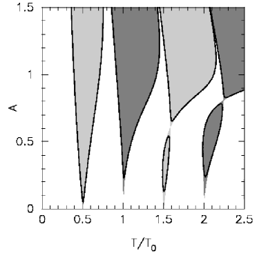
FIG. 2.: Shaded regions indicate $R>1$ (darker) and $R<-1$ (lighter). Solid lines delineate the boundaries $|R|=R_{c}$. The damping $\gamma=0.01$ and the frequency $\omega_{0}=0.4$.

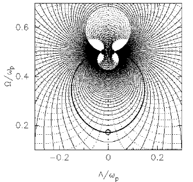
FIG. 3.: Contour plots of the left-hand side of Eq. (38) (solid lines) and Eq. (39) (broken lines) for $\omega_{0}=0.4$, $k=1.28$, $\gamma=0.01$, $A=1.0$, and $T_{k}=2T_{p}$, which lead to $R=1.00617$. Poles of a single oscillator are indicated by solid circles. Thick lines correspond to solutions of Eqs. (38) (solid) and (39) (broken). The intersections of the solid and dotted thick lines, indicated by open circles, are thus solutions of Eq. (30). Although there is a single oscillator pole with positive $\Lambda$ there is no positive-$\Lambda$ collective mode.

FIG. 4.: Trajectories associated with Fig. 3. Thick solid line: mean $\left<x\right>$. Thin solid line: deviation $\Delta x$. The inset also includes the trajectory $x$ of an individual oscillator (broken line).

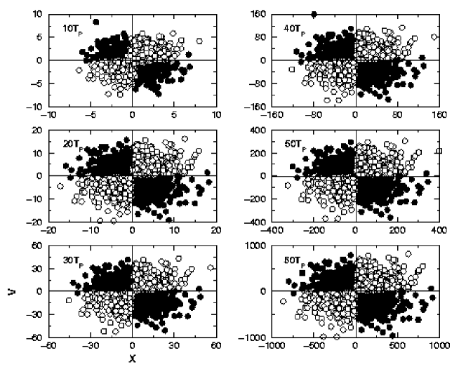
FIG. 5.: Phase point snapshots of $2000$ individual oscillators in the system associated with Figs. 3 and 4. Note the scale changes with increasing time.

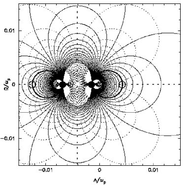
FIG. 6.: Contour plots of the left-hand side of Eqs. (38) (solid lines) and Eq. (39) (broken lines) for $\omega_{0}=0.4$, $k=1.28$, $\gamma=0.01$, $A=1.0$, and $T_{k}=T_{p}$, which lead to $R=1.0001$. Poles of a single oscillator are indicated by solid circles. Thick lines correspond to solutions of Eqs. (38) (solid) and (39) (broken). The intersections of the solid and dotted thick lines, indicated by open circles, are thus solutions of Eq. (30). Although the single oscillator poles have all negative $\Lambda$, the collective modes include a pole with positive $\Lambda$ and $\Omega=0$. This mode diverges exponentially without oscillation.

FIG. 7.: Trajectories associated with Fig. 6. Thick solid line: mean $\left<x\right>$. Thin solid line: deviation $\Delta x$. The inset also includes the trajectory $x$ of an individual oscillator (broken line).

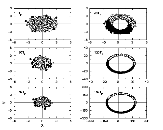
FIG. 8.: Phase point snapshots of $2000$ individual oscillators in the system associated with Figs. 6 and 7. Note the scale changes with increasing time.

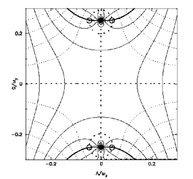
FIG. 9.: Contour plots of the left-hand side of Eqs. (38) (solid lines) and Eq. (39) (broken lines) for $\omega_{0}=0.4$, $k=1.28$, $\gamma=0.01$, $A=1.0$, and $T_{k}=4T_{p}/3$, which lead to $R=-0.01037$. Poles of a single oscillator are indicated by solid circles. Thick lines correspond to solutions of Eqs. (38) (solid) and (39) (broken). The intersections of the solid and dotted thick lines, indicated by open circles, are thus solutions of Eq. (30). Although the single oscillator poles all have negative $\Lambda$, the collective modes include a pole with positive $\Lambda$ and nonzero. This mode diverges exponentially with oscillation.

FIG. 10.: Trajectories associated with Fig. 9. Thick solid line: mean $\left<x\right>$. Thin solid line: deviation $\Delta x$. The inset also includes the trajectory $x$ of an individual oscillator (broken line).

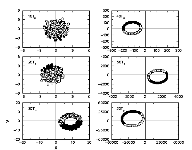
FIG. 11.: Phase point snapshots of $2000$ individual oscillators in the system associated with Figs. 9 and 10. Note the scale changes with increasing time.

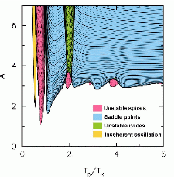
FIG. 12.: Phase diagram for the mean field model with oscillator parameters $\omega_{0}=0.4$, $k=1.28$ and $\gamma=0.16$. White regions denote stable regimes. The various instability regimes are color coded as indicated. The characteristic behavior in each instability regime is described in the text.

FIG. 13.: Bifurcation diagrams showing $\Lambda$ (solid lines) and $\Omega$ (dotted lines) with changing modulation amplitude for various values of the modulation period. Panel (a): $T_{p}/T_{k}=0.75$; (b): $T_{p}/T_{k}=2.04$; (c): $T_{p}/T_{k}=3.0$; (d): $T_{p}/T_{k}=3.9$. The behavior implied by these diagrams is discussed in detail in the text.

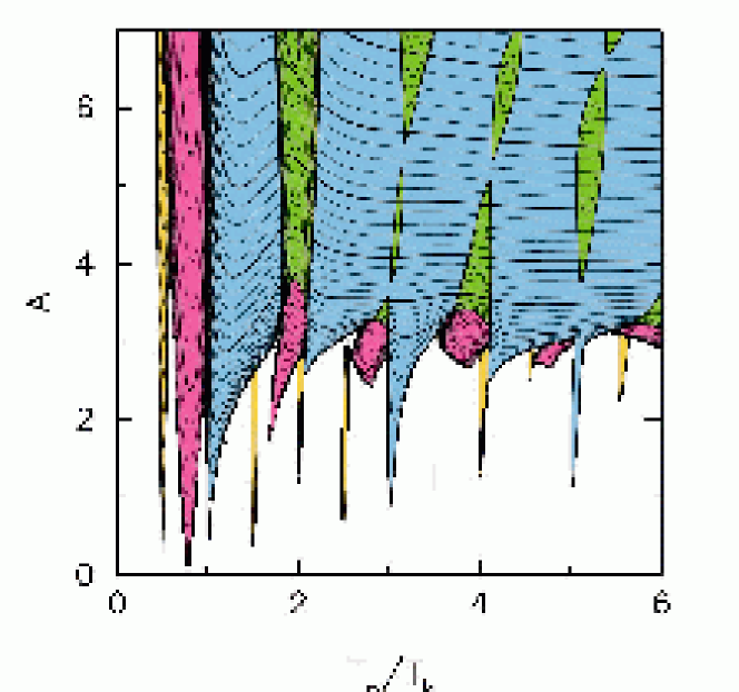
FIG. 14.: Phase diagram for the mean field model with oscillator parameters $\omega_{0}=0.4$, $k=1.28$ and $\gamma=0.01$.

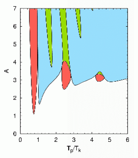
FIG. 15.: Bifurcation diagram for the anti-phased dimer with the same parameters as in Fig. 12

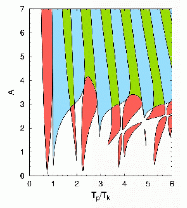
FIG. 16.: Phase diagram for the anti-phased dimer with the same parameters as in Fig. 14

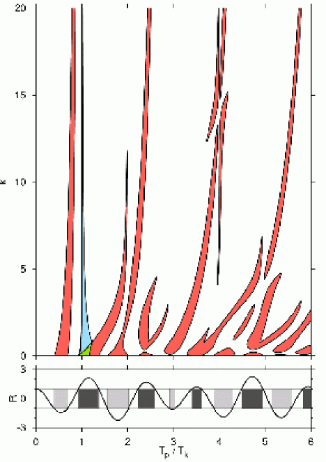
FIG. 17.: Upper panel: Bifurcation diagram for the anti-phased dimer in the $(T_{p}/T_{k},k)$ plane for $A=0.9$, $\gamma=0.01$, and $\omega_{0}=0.4$, using the same color convention as in Fig. 12. Lower panel: $R$ (Eq. (13)) as a function of $T_{p}/T_{k}$; light grey areas denote $R<-1$ and dark grey areas $R>1$.

REFERENCES

- [1] Y. Kuramoto, Chemical Oscillations, Waves and Turbulence (Springer, Berlin, 1984).
- [2] I. Bena and C. Van den Broeck, Europhys. Lett. 48, 498 (1999).
- [3] M. Copelli and K. Lindenberg, to appear in Phys. Rev. E, cond-mat/0008022.
- [4] R. Kawai et al., in preparation.
- [5] L. D. Landau and E. M. Lifschitz, Mechanics, (Pergamon Press, Oxford, 1969); V.I. Arnold, Equations différentielles ordinaires (Editions Mir, Moscou, 1974).
- [6] K. Lindenberg, V. Seshadri, and B.J. West, Phys. Rev. A 22, 2171 (1980); N. G. van Kampen, Stochastic Processes in Physics and Chemistry (North Holland, Amsterdam, 1981), p. 382, 387 and 393; Abdullaev, S. Darmanyan and M. Djumaev, Phys. Lett. A141, 423 (1989); P. S. Landa and A. A. Zaikin, Phys. Rev. E 54, 3535 (1996); P. S. Landa, A. A. Zaikin, M. G. Rosenblum and J. Kurths, Phys. Rev. E 56, 1465 (1997).
- [7] R. M. Mazo, J. Stat. Phys. 24, 39 (1981); M. Gitterman, R. J. Schrager and G. H. Weiss, Phys. Lett. A 142, 84 (1989); C. Zerbe, P. Jung and P. Hänggi, Phys. Rev. E 49, 3626 (1994).
- [8] Such parametric oscillators are encountered in a variety of contexts that include elementary particles, astrophysics, fluid mechanics, magnetism, plasma physics, electrical and electronic networks, optical systems and lasers, applied mechanics, and biophysics, cf. bibliography in [2] and [3].
- [9] J. Tan and G. Gabrielse, Phys. Rev. Lett. 67, 3090 (1991).
- [10] P. Coullet and K. Emilsson, Physica D 61, 119 (1992); V. Petrov, Q. Ouyang and H. L. Swinney, Nature 388, 655 (1997).
- [11] A. H. Nayfeh and D. T. Mook. Nonlinear Oscillations (Wiley, New York, 1979).
- [12] B. Denardo et al. , Phys. Rev. Lett. 68, 1730 (1992); N. V. Alexeeva, I. V. Barashenkov, and G. P. Tsironis, Phys. Rev. Lett. 84, 3053 (2000).
- [13] B. Van der Pol and M. J. O. Strutt, Phil. Mag. 5, 18 (1928).
- [14] E. Yorke, Am. J. Phys. 46, 285 (1978).
- [15] K. Lindenberg and B. J. West, The Nonequilibrium Statistical Mechanics of Open and Closed Systems (VCH, New York, 1990).
- [16] C. Van den Broeck and I. Bena, “Parametric resonance revisited,” preprint.
- [17] C. Van den Broeck and R. Kawai, Phys. Rev. E 57, 3866 (1998).
- [18] A. Becker and L. Kramer, Phys. Rev. Lett. 73, 955 (1994); G. Grinstein. M. A. Munoz and T. Yuhai, Phys. Rev. Lett. 76, 4376 (1996).
- [19] As opposed to the anti-phased dimer, the phased dimer () can reproduce the yellow regions exactly [3].