New correlation duality relations for the planar Potts model

Abstract

We introduce a new method to generate duality relations for correlation functions of the Potts model on planar graphs. The method extends previously known results, by allowing the consideration of the correlation function for arbitrarily placed vertices on the graph. We show that generally it is linear combinations of correlation functions, not the individual correlations, that are related by dualities. The method is illustrated in several non-trivial cases, and the relation to earlier results is explained. A graph-theoretical formulation of our results in terms of rooted dichromatic, or Tutte, polynomials is also given.

1 Introduction

The Potts model, a generalization of the Isling model to $q$ spin components introduced by Potts [1] in 1952, has been at the forefront of research interest for almost five decades. While the critical properties of planar models are now largely known [2] - [5], much less is known about their correlation functions.

A key element of planar spin models is the notion of duality relations. Every planar graph, or lattice, $G$ has an associated dual planar graph $G^{(\rm D)}$, and it is well-known [1, 6] that the partition functions of the Potts model on $G$ and $G^{(\rm D)}$ are proportional to each other when their couplings are correctly related. In the case of $q=2$, the Ising model, it is also known [7] that a duality relation exists between certain two-spin correlation functions. It has long been suspected that the correlations of the Potts models on $G$ and $G^{(\rm D)}$ should be similarly related. Indeed, in a series of recent papers we have obtained correlation dualities for vertices (spins) residing on the boundary of one face [8] - [10] or two faces [11] of $G$, and reformulated the 1–face results in graph-theoretical terms [12]. In this paper we consider the $N$-face problem, namely, correlation duality relations for vertices residing on $N$ faces of $G$ for general $N$. As we shall see, a new picture emerges for $N\geq 2$. Instead of duality relations between individual correlation functions, we now obtain relations between linear combinations of correlation functions.

The organization of this paper is as follows. In Sec. 2 we establish notations and briefly review the Fortuin-Kasteleyn (F-K) representation of the Potts model, and derive the duality relation for the partition function. Using two identities which we establish as lemmas, we introduce in Section 3 a method which allows us to generate correlation duality relations. While our method does not necessarily generate all such duality relations, we show that generally the duality relates linear combinations of, rather than individual, correlation functions. Explicit examples are given in Section 4 and the relation to earlier results is explained. In Section 5 we reformulate our results in graph-theoretical terms as rooted dichromatic, or Tutte, polynomials.

2 The setup

2.1 The Fortuin-Kasteleyn representation

Consider a finite, planar connected graph $G$ with vertex set $V$, edge set $E$, and face set $F$. We write $|V|$ for the size of the set $V$ and similarly for $E$, $F$, and other terms. Let $\sigma$ denote an assignment of colors, or states, to the vertices of $G$, which is a map from $V$ to the color set ${\cal C}=\{1,\dots,q\}$. Then the partition function of the Potts model on $G$ is

$$Z=\sum_{\sigma}\,\prod_{\langle i,j\rangle}\,e^{K\delta({\sigma}_{i},{\sigma}_{j})}$$ (1)

where the summation is over the $|V|^{q}$ coloring assignments $\sigma$, the product runs over all nearest neighbor spin pairs interacting with the coupling parameter $K$, $\delta$ is the Kronecker delta function, and $\sigma_{i}$ is the color of the $i$-th vertex.

The Fortuin-Kasteleyn (F-K) representation [13] of the Potts model replaces the configurational sum in (1) by a sum over edge sets. Let $S\subseteq E$ be an edge set on the graph $G$. If we remove from $G$ all the edges which are not in $S$, we obtain a subgraph which contains all the vertices, and which in general has many connected components. This is called a spanning subgraph of $G$. We write $|S|$ to denote the number of edges in $S$, and write $p(S)$ to denote the number of connected components in the spanning subgraph defined by $S$. In this picture, any isolated vertex in the spanning subgraph counts as a connected component, and so contributes a summand 1 in the counting of $p(S)$. Define

$$v=e^{K}-1$$ (2)

so that we have

$$e^{K\delta({\sigma}_{i},\sigma_{j})}=1+v\,\delta({\sigma}_{i},\sigma_{j})$$ (3)

The substitution of (3) into (1) now gives rise to the F-K representation of the partition function

$$Z(G;q,v)\equiv Z=\sum_{S\subseteq E}v^{|S|}\,\,q^{p(S)}$$ (4)

The number of colors $q$ appears as a variable in (4), rather than a summation limit as in (1). For this reason the F-K representation (4) forms the basis of essentially all analyses of the Potts model.

2.2 Dual partition functions

As a precursor to discussions in later sections, we give here a graph-theoretical derivation of the well-known duality relation for the partition function.

The standard dual graph of $G$ is constructed by placing vertices in the faces of $G$, and connecting them with edges which are transverse to the edges of $G$. A pair of transverse edges are said to be dual to each other. The resulting dual graph $G^{(\rm D)}$ has $|F|$ vertices, $|E|$ edges and $|V|$ faces, and is also planar. For a given edge set $S$ on $G$, we define its dual edge set $S^{(\rm D)}$ on $G^{(\rm D)}$ by requiring that an edge of $G^{(\rm D)}$ is in $S^{(\rm D)}$ if and only if its dual edge is not in $S$. Thus,

$$|S|+|S^{(\rm D)}|=|E|$$ (5)

Moreover, if we start from $|V|$ isolated vertices of $G$, and add one by one the edges of $S$, then each edge reduces $p(S)$ by 1 unless it forms an independent cycle, in which case $p(S)$ is unchanged. Therefore we have the relation

$$p(S) = |V|-|S|+c(S)$$ (6)

$$= |V|-|S|+p(S^{(\rm D)})-1$$

where $c(S)$ is the number of independent cycles in the spanning subgraph of $S$, and is related to $p(S^{(\rm D)})$, the number of components in $S^{(\rm D)}$, through the topological relation $c(S)=p(S^{(\rm D)})-1$. Using (5) and (6) we have the identity

$$v^{|S|}\,q^{p(S)} = v^{|E|-|S^{(\rm D)}|}q^{|V|-|S|+p(S^{(\rm D)})-1}$$ (7)

$$= k\,(q/v)^{|S^{(\rm D)}|}\,q^{p(S^{(\rm D)})}$$

where

$$k=q^{1-|F|}v^{|E|}$$ (8)

and we have used the Euler relation

$$|V|+|F|=|E|+2$$ (9)

Substituting (7) into (4), we see that the Potts model partition functions on $G$ and $G^{(\rm D)}$ are proportional, when the couplings $K$ and $K^{*}$ are related by the equation

$$vv^{*}=q$$ (10)

where $v^{*}=e^{K^{*}}-1$. The partition function duality is the statement that

$$Z(G;q,v)=k\,Z(G^{(\rm D)};q,v^{*})$$ (11)

where we have made use of the one-to-one correspondence between edge sets $S$ and dual edge sets $S^{(\rm D)}$. Note that we have

$$k\cdot k^{(\rm D)}=q^{1-|F|}v^{|E|}\cdot q^{1-|V|}(v^{*})^{|E|}=1$$ (12)

which says that the dual of the dual partition function is the partition function itself.

2.3 The correlation function

The Potts correlation function is defined as the probability that a given set of vertices are assigned fixed colors [4]. Specifically, let $R\subseteq V$ be any subset of the vertices which are assigned fixed colors. We shall call these the roots for the correlation functions, and the graph with roots a rooted graph. Let the $|R|$ roots lie on the boundaries of $N$ distinct faces of $G$, which will be called the external faces of the graph. For simplicity, we shall assume that external faces are not adjacent to each other, namely they do not share any vertices or boundary edges.

Let $c:R\rightarrow{\cal C}$ be any assignment of colors on the roots, so that $c_{i}$ is the color assigned to the root $i$, and we write

$${\delta}_{c}(\sigma)=\prod_{i\in R}{\delta}(\sigma_{i},{c}_{i})$$ (13)

Then the correlation function for the assignment $c$ on the root set $R$ is defined to be the expectation value of $\delta_{c}(\sigma)$, namely,

$$P_{c}\equiv\langle{\delta}_{c}(\sigma)\rangle=Z(G;q,v)^{-1}{\sum_{\sigma}}\,{\delta}_{c}(\sigma)\prod_{\langle i,j\rangle}\,e^{K\delta({\sigma}_{i},\sigma_{j})}$$ (14)

where the summation in the right-hand side is a partial partition function. Clearly, the explicit expression of $P_{c}$ depends on the location of the roots as well as the explicit color assignment $c$.

Every color assignment $c$ defines a partition $X$ of the roots, namely a division of the $|R|$ roots into disjoint blocks, by the rule that two vertices $i,j$ in $R$ belong to the same block of $X$ if and only if $c_{i}=c_{j}$. By the symmetry of the Potts interactions, the correlation (14) depends only on this partition defined by $c$, not on the specific colors. We can therefore associate each partial partition function to a partition $X$. Alternately, for any partition $X$ of the roots, we have a partial partition function

$$Z_{X}\equiv Z_{X}(G;q,v)={\sum_{\sigma}}\,{\delta}_{c}(\sigma)\prod_{\langle i,j\rangle}\,e^{K\delta({\sigma}_{i},\sigma_{j})}$$ (15)

where $c$ is any color assignment that produces the partition $X$. Since $P_{c}$ and $Z_{X}$ are proportional, it is sufficient to discuss duality relations for the partial partition function $Z_{X}$.

The F-K representation also extends to the partial partition functions. For any edge set $S$, we define a “connected” partition $\pi(S)$ of $R$ by the rule that two roots $i,j$ belong to the same block if and only if they belong to the same connected component of the spanning subgraph defined by $S$. Using this notion, we can separate the edge sets into classes

$${\cal S}(X)=\{S\subseteq E\,:\,\pi(S)=X\}$$ (16)

labeled by their corresponding connected partitions of $R$. Clearly every edge set $S$ belongs to exactly one of these classes ${\cal S}(X)$.

Now the role of the factor $\delta_{c}(\sigma)$ in (14) and (15) is to restrict the summations to fixed colors for vertices in $R$. The net result is that each cluster containing roots contributes a factor 1, instead of the factor $q$ in (4). This leads us to define, for any partition $X$, the summation over edge sets $S$ with $\pi(S)=X$,

$$F_{X}(G;q,v)=\sum_{S\in{\cal S}(X)}v^{|S|}\,\,q^{p(S)-|X|},$$ (17)

where $|X|$ is the number of blocks in $X$. The set of partitions of $R$ is partially ordered. We write $Y\preceq X$ to mean that every block in $Y$ is wholly contained in a block in $X$ or, equivalently, $Y$ is a refinement of $X$. Then we have the identity

$$Z_{X}(G;q,v)=\sum_{Y\preceq X}F_{Y}(G;q,v)$$ (18)

2.4 Möbius inversion and planar identities

It is well-known [14] that the partially ordered sum (18) can be inverted, allowing us to write $F_{X}$ as a linear combination of $Z_{Y}$. For $Y\preceq X$ define the Möbius inversion coefficient

$$\mu(Y,X)=(-1)^{|Y|-|X|}\prod_{b\in X}(n_{b}(Y)-1)!$$ (19)

where the product on the right side runs over blocks $b$ in $X$, and $n_{b}(Y)$ is the number of blocks of $Y$ that are contained in $b$. Then we have for every partition $X$,

$$F_{X}(G;q,v)=\sum_{Y\preceq X}\mu(Y,X)Z_{Y}(G;q,v)$$ (20)

One peculiarity for planar graphs is that $F_{X}$ can be zero for certain partitions $X$. This phenomenon was explored in detail in [10] in the case of a single external face. In this case, one has $F_{X}=0$ if the partition $X$ is non-planar (also called a crossing partition in the mathematics literature [15]). It then follows from (20) that whenever $X$ is a non-planar partition, the partial partition functions $Z_{Y}$ must satisfy the identity

$$\sum_{Y\preceq X}\mu(Y,X)Z_{Y}(G;q,v)=0$$ (21)

giving rise to “sum-rule” relations for the partial partition functions [9]. In general, when there are several external faces, identities of this type also hold for any root set $R$, although it seems to be a hard problem to decide if a given partition is planar or not.

3 Correlation duality relation

3.1 Dual rooted graph $G^{*}$

In Section 2.2 we introduced the dual graph $G^{(\rm D)}$, and described the well-known duality for partition functions on $G$ and $G^{(\rm D)}$. In this section we introduce the dual rooted graph $G^{*}$ which plays the corresponding role for correlation functions.

Starting from a rooted graph with $|R|$ roots on $N$ external faces, one can construct a dual rooted graph $G^{*}$. The procedure of constructing $G^{*}$ for $N=1$ has been described in detail in [10, 12]. The construction of $G^{*}$ for general $N$ repeats the $N=1$ process for each external face, a prescription we now briefly describe.

Place $N$ extra vertices, one each in the center of each of the $N$ external faces. For each external face, let $f$ be the extra vertex and connect it to each root on the boundary of this face by an edge. This gives a new graph $G^{\prime\prime}$ which has $N$ more vertices than $G$ and $|R|$ additional edges. The dual graph of $G^{\prime\prime}$ is also planar, and it has $N$ faces containing the $N$ extra vertices $f$. Now remove all edges of these $N$ faces, and the resulting graph is the dual rooted graph $G^{*}$.

The vertices of $G^{*}$ residing inside the $N$ external faces of $G$ are now the dual roots and we denote this set by $R^{*}$. Clearly, the number of edges of $G^{*}$ is $|E|$, and we have $|R^{*}|=|R|$ (because external faces are non-adjacent). It is also clear that the total number of vertices of $G^{*}$ is

$$|V^{*}|=|F|+|R|-N$$ (22)

We can recover the standard dual graph $G^{(\rm D)}$ from $G^{*}$ by fusing the dual roots $R^{*}$ inside each external face into a single dual vertex. This gives a one-to-one correspondence between edges on $G^{(\rm D)}$ and $G^{*}$, and hence we define the dual edge set $S^{*}$ on $G^{*}$ to be the same edge set as $S^{(\rm D)}$ on $G^{(\rm D)}$. Therefore in particular we have

$$|S^{*}|=|S^{(\rm D)}|$$ (23)

Let $G^{(\rm F)}$ denote the graph generated by fusing all roots $R$ in $G$, and $({G^{*}})^{(\rm F)}$ the graph generated by fusing all roots $R^{*}$ in $G^{*}$. Then, we have the identities

$$({G^{*}})^{(\rm F)}=G^{(\rm D)}\hskip 14.22636pt{\rm and}\hskip 14.22636ptG^{(\rm F)}=(G^{*})^{(\rm D)}$$ (24)

3.2 A preliminary relation

Our results will depend crucially on the topology of the connectedness of the partitions $\pi(S)$ and $\pi(S^{*})$. Fix an edge set $S$ on $G$, and let $X=\pi(S)$, $Y=\pi(S^{*})$. Recall that $|X|$ is the number of blocks in $X$. Also, let $n(X)$ be the number of clusters of external faces on $G$ connected by $S$ (where we define two external faces to be in the same cluster if a connected component of $S$ contains roots on both faces). Similar definitions apply to $|Y|$ and $n(Y)$.

Now $S^{*}$ and $S^{(\rm D)}$ are the same edge set, and $G^{(\rm D)}$ is obtained from $G^{*}$ by fusing. Hence we have

$$p(S^{*}) = |Y|+\Delta$$

$$p(S^{(\rm D)}) = n(Y)+\Delta$$ (25)

where $\Delta$ is the number of connected components in the spanning graph generated by $S^{*}$ that are not connected to any dual roots. It follows that we have

$$|Y|-n(Y)=p(S^{*})-p(S^{(\rm D)})$$ (26)

and similarly

$$|X|-n(X)=p(S)-p({S^{*}}^{(\rm D)})$$ (27)

where ${S^{*}}^{(\rm D)}$ on ${G^{*}}^{(\rm D)}$ is the edge set dual to $S^{*}$ on $G^{*}$. Combining (26) and (27) and making use of (6), we obtain the identity

$$|X|+|Y|-n(X)-n(Y) = [p(S)-p(S^{(\rm D)})]+[p(S^{*})-p({S^{*}}^{(\rm D)})]$$ (28)

$$= [|V|-|S|-1]+[|V^{*}|-|S^{*}|-1]$$

$$= |V^{*}|-|F|$$

$$= |R|-N$$

where use has also been made of (22), the Euler relation (9), and the relation

$$|S|+|S^{*}|=|E|$$ (29)

For $N=1$, we have $n(X)=n(Y)=1$, and (28) reduces to

$$|X|+|Y|=|R|+1$$ (30)

a relation used in [10]. For $N=2$, (28) reduces to Eq. (21) of Ref. [11].

3.3 First identity

Our construction of correlation duality relations is based on the use of two identities. The first identity, which we now state as a lemma, is a generalization of the identity (7). The new ingredient here is that the generalization should permit the consideration of the factor $v^{|S|}\,\,q^{p(S)-|X|}$ appearing in the F-K representation (17).

Lemma 1

For a fixed edge set $S$ on $G$, define $X=\pi(S)$ and $Y=\pi(S^{*})$. Then we have the identity

$$v^{|S|}\,\,q^{p(S)-[|X|-n(X)]/2}=k^{\prime}\,\,(v^{-1}q)^{|S^{*}|}\,\,q^{p(S^{*})-[|Y|-n(Y)]/2}$$ (31)

where

$$k^{\prime}=v^{|E|}\,q^{1-|F|-[|R|-N]/2}$$ (32)

Remark: Notice that $v^{-1}q=e^{K^{*}}-1$, so we define $v^{*}=v^{-1}q$ as before, and we can rewrite (31) as follows to indicate the explicit dependence on $S$ and $S^{*}$,

$$v^{|S|}\,\,q^{p(S)-[|\pi(S)|-n(\pi(S))]/2}=k^{\prime}\,\,(v^{*})^{|S^{*}|}\,\,q^{p(S^{*})-[|\pi(S^{*})|-n(\pi(S^{*}))]/2}$$ (33)

Proof: The proof of the lemma parallels that of the partition function duality given in Section 2.2. First, the relation (6) still holds so that after using (29) the first line of (7) becomes

$$v^{|S|}\,q^{p(S)}=v^{|E|-|S^{*}|}q^{|V|-|S|+p(S^{(\rm D)})-1}$$ (34)

The lemma (31) now follows after the use of the identities (26) and (28). Notice that we have

$$k^{\prime}\cdot(k^{\prime})^{*}=v^{|E|}\,q^{1-|F|-[|R|-N]/2}\cdot(v^{*})^{|E|}\,q^{1-|V^{*}|-[|R|-N]/2}=1$$ (35)

where $|V^{*}|$, the number of faces of the dual of $G^{*}$, is given by (22).

3.4 Second identity

Let $S$ and $T$ be edge sets which define the same partition of $R$, i.e., $\pi(S)=\pi(T)$, then a key feature of the case $N=1$ is that their dual edge sets also define the same partition of $R^{*}$. Namely,

$$\pi(S)=\pi(T){\rm\ \ \ \ if,\>\>and\>\>only\>\>if\ \ \ \ }\pi(S^{*})=\pi(T^{*}),\hskip 28.45274ptN=1$$ (36)

This feature permits us to derive correlation duality relations for $N=1$ [8] - [10]. But (36) is false for $N\geq 2$ [11]. However a weaker statement holds which we now state as a lemma.

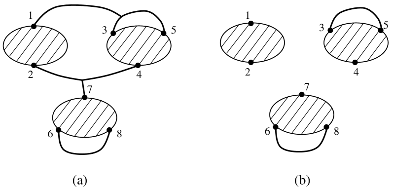
Figure 1: An $N=3$ example of a partition $X$ and the associated local partition $X_{\rm loc}$. (a) $X=(135)(247)(68)$, (b) $X_{\rm loc}=(1)(35)(2)(4)(7)(68)$. Cross-hatched areas denote external faces; lines denote connected edge sets.

First, some definitions: A block of $X$ is local if it contains roots from one face only, and is non-local otherwise. A partition $X$ is local if every block of $X$ is local, and is non-local if any block in $X$ is non-local. Given a partition $X$, we can construct from it a unique local partition $X_{\rm loc}$ as follows: We split up every non-local block into a collection of local blocks, by separating its roots which lie on different faces. The collection of all these local blocks is the new partition $X_{\rm loc}$. See Fig. 1 for an example.

Any local partition is a collection of planar partitions of the roots on each of the external faces. Each of these planar partitions on a single face has a unique dual partition. So for any local partition $\xi=X_{\rm loc}$, we will define ${\xi}^{*}$ to be the collection of these dual partitions on $G^{*}$, and by extension we will call it the dual partition of $\xi$. Notice that ${\xi}^{*}$ is always a local partition on $G^{*}$.

Lemma 2

For any edge set $S$ on $G$, we have

$$\pi(S^{*})_{\rm loc}\preceq\pi(S)_{\rm loc}^{*}$$ (37)

Furthermore, let $S$ and $T$ be two edge sets on $G$, and suppose that $\pi(S)=\pi(T)$. Then we have

$$\pi(S^{*})_{\rm loc}=\pi(T^{*})_{\rm loc}$$ (38)

Remark: The result corresponding to (38) also holds on $G^{*}$, namely, if $\pi(S^{*})=\pi(T^{*})$ then also $\pi(S)_{\rm loc}=\pi(T)_{\rm loc}$.

Proof: It is sufficient to establish the relations (37) and (38) for each external face separately. So pick one external face, call it $f$, and let $R_{f}$ denote the roots which belong to this face, and $R_{f}^{*}$ their dual roots. We will construct two different $N=1$ rooted graphs from $(G,R)$, as follows (recall that a rooted graph is an ordered pair, consisting of a graph together with a set of roots. Mostly we have ignored the distinction between graph and rooted graph, but we will distinguish them throughout this proof).

First, by ignoring the roots on the other faces we obtain the rooted graph $(G,R_{f})$. As a shorthand we will denote this pair by $G_{f}$. Second, by fusing the roots on the other external faces (but not on $f$) we obtain a different rooted graph $(G^{(F)}_{f},R_{f})$, which also has roots only on the face $f$. (Recall that we fuse roots on a face by merging them into a single vertex). Again as a shorthand we denote this by $G^{F}_{f}\equiv(G^{(F)}_{f},R_{f})$.

Each of these rooted graphs has a dual rooted graph, which we denote by $G_{f}^{*}$ and $(G^{F}_{f})^{*}$ respectively. These are constructed according to the procedure described in Section 3.1 for the $N=1$ case, using only the roots on the face $f$. Notice that the underlying graph of $(G^{F}_{f})^{*}$ is identical to the graph $G^{*}$, because the process of fusing roots on a face in $G$ automatically splits the dual vertex in $G^{(\rm D)}$ to produce the dual roots. As a convenient shorthand we write $(G^{*})_{f}$ to denote the pair $(G^{*},R_{f}^{*})$, which is obtained from $G^{*}$ by ignoring the roots on the other faces. It follows then that

$$(G^{F}_{f})^{*}=(G^{*})_{f}$$ (39)

Now let $S$ be an edge set on $G$. Since the underlying graphs of $G_{f}$ and $G^{F}_{f}$ have the same edges as $G$, $S$ also defines partitions of the roots $R_{f}$ on $G_{f}$ and $G^{F}_{f}$. For clarity in this proof, we write these partitions as $\pi(S;G_{f})$ and $\pi(S;G^{F}_{f})$ respectively, where we include the graph in order to distinguish them. Note that $\pi(S;G_{f})$ is one part of the local partition $\pi(S)_{\rm loc}$, namely the part that contains the roots on $f$. Let $\pi(S)_{f}$ denote this part of the partition $\pi(S)_{\rm loc}$, and similarly $\pi(S^{*})_{f}$ the part of $\pi(S^{*})_{\rm loc}$ which contains the dual roots on $f$. So we have

$$\pi(S;G_{f})=\pi(S)_{f},\quad\quad\pi(S^{*};(G^{*})_{f})=\pi(S^{*})_{f}$$ (40)

To prove the first result (37), note that since $G^{F}_{f}$ is obtained from $G_{f}$ by fusing vertices we have

$$\pi(S;G_{f})\preceq\pi(S;G^{F}_{f})$$ (41)

These are both $N=1$ partitions, hence they have dual partitions, and these satisfy

$$\pi(S;G_{f})^{*}\succeq\pi(S;G^{F}_{f})^{*}=\pi(S^{*};(G^{F}_{f})^{*})$$ (42)

Using (39) and (40) this gives

$$\pi(S)_{f}^{*}=\pi(S;G_{f})^{*}\succeq\pi(S^{*};(G^{*})_{f})$$ (43)

Combining these for every external face gives

$$\pi(S)_{\rm loc}^{*}\succeq\pi(S^{*})_{\rm loc}$$ (44)

To prove the second result (38), note that since $\pi(S)=\pi(T)$ it follows also that

$$\pi(S;G^{F}_{f})=\pi(T;G^{F}_{f}).$$ (45)

Taking the dual of both sides gives

$$\pi(S^{*};(G^{F}_{f})^{*})=\pi(T^{*};(G^{F}_{f})^{*})$$ (46)

and hence

$$\pi(S^{*};(G^{*})_{f})=\pi(T^{*};(G^{*})_{f})$$ (47)

Again combining these for every external face gives

$$\pi(S^{*})_{\rm loc}=\pi(T^{*})_{\rm loc}$$ (48)

Q.E.D.

3.5 Form of duality relations

As a convenient shorthand, for partitions $X$ of $R$ and $Y$ of $R^{*}$ we write

$$Z_{X}=Z_{X}(G;q,v),\hskip 28.45274ptZ_{Y}^{*}=Z_{Y}(G^{*};q,v^{*})$$ (49)

and similarly we write

$$F_{X}=F_{X}(G;q,v),\hskip 28.45274ptF_{Y}^{*}=F_{Y}(G^{*};q,v^{*})$$ (50)

where $F_{X}$ is defined in (18). We seek duality relations which express each given $Z_{X}$ in terms of a linear combination of the dual $Z_{Y}^{*}$. Recall the Möbius inversion (20) relating $Z_{X}$ to $F_{X}$, it is sufficient to obtain duality relations for the functions $F_{X}$. Indeed, for $N=1$, for example, the identity (36) ensures that there is a one-to-one correspondence between the (connected) partitions $X=\pi(S)$ on $G$ and $Y=\pi(S^{*})$ on $G^{*}$. Then, using Lemma 1 one obtains the desired duality relation

$$q^{|X|/2}F_{X}(G;q,v)=k^{\prime}\ q^{|Y|/2}F_{Y}(G^{*};q,v^{*})\hskip 28.45274ptN=1$$ (51)

where we have used $n(X)=n(Y)=1$, and the coefficient $k^{\prime}$ was defined in (32). This duplicates a result of [10].

For $N\geq 2$, however, the mappings $X\to Y$ and/or $Y\to X$ are not necessarily one-to-one [11]. See Fig. 2 for an example. Generally, for fixed $\pi(S)=X,\pi(S^{*})=Y$, we define by analogy to (17) the functions

$$F_{X,Y}(G;q,v) = \sum_{S\in{\cal S}(X),S^{*}\in{\cal S}(Y)}v^{|S|}\,\,q^{p(S)-|X|}$$

$$F_{Y,X}(G^{*};q,v^{*}) = \sum_{S\in{\cal S}(X),S^{*}\in{\cal S}(Y)}{(v^{*})}^{|S^{*}|}\,\,q^{p(S^{*})-|Y|},$$ (52)

Then, one has the duality relation

$$q^{|X|/2}F_{X,Y}(G;q,v)=k^{\prime}\ q^{|Y|/2}F_{Y,X}(G^{*};q,v^{*})$$ (53)

which is a generalization of (51). The partial partition functions are then

$$Z_{X}(G;q,v) = \sum_{X^{\prime}\preceq X}\sum_{Y}F_{X,Y}(G;q,v)$$

$$Z_{Y}(G^{*};q,v^{*}) = \sum_{Y^{\prime}\preceq Y}\sum_{X}F_{Y,X}(G^{*};q,v^{*})$$ (54)

For $N=1$, the $X\leftrightarrow Y$ mapping is unique, so that (3.5) becomes (18) and the relation (3.5) can be inverted, permitting one to express $Z_{X}$ as a linear combination of $Z_{Y}$’s. For $N\geq 2$, however, (3.5) cannot be inverted, and so we cannot express the $F_{X,Y}$ in terms of the $Z_{X}$. Hence the duality relations (53) do not help us. As a result, we will instead derive duality relations of the form

$$\sum_{X}\alpha(X)F_{X}=k^{\prime}\,\sum_{Y}\beta(Y)F_{Y}^{*}$$ (55)

The sum on the left runs over partitions of the root set $R$, and the sum on the right side runs over partitions on $R^{*}$. The coefficients $\alpha$ and $\beta$ depend on $q,v$ as well as their arguments $X$ and $Y$, and are different for each duality relation.

Using the Möbius inversion (20), (55) provides duality relations for the partial partition functions, and we end up with

$$\sum_{W}a(W)Z_{W}=k^{\prime}\,\sum_{U}b(U)Z_{U}^{*},$$ (56)

where

$$a(W) = \sum_{X\succeq W}\mu(W,X)\alpha(X)$$

$$b(U) = \sum_{Y\succeq U}\mu(U,Y)\beta(Y)$$ (57)

Note that the number of independent relations depends on the root set $R$. If all roots lie on one face, so that $N=1$, then our result produces the same number of relations as the number of planar partitions of the root set. This duplicates the results of [10]. If all roots lie on distinct faces, so that $|R|=N$, then our method produces just one relation, namely the original duality (11).

3.6 Correlation duality

We use the two lemmas to generate correlation duality relations. The definition (3.5) was not useful because it involved a sum over all edge sets $S$ with fixed partition $X=\pi(S)$ and fixed dual partition $Y=\pi(S^{*})$. As we now show, one way to generate duality relations is by summing instead over all edge sets with fixed local partitions $X_{\rm loc}$ and $Y_{\rm loc}$. According to (37) each of these must be a refinement of the dual of the other, so we can restrict attention to such pairs of local partitions.

Accordingly, writing

$$\xi=X_{\rm loc},\hskip 28.45274pt\eta=Y_{\rm loc}$$ (58)

we say that $(\xi,\eta)$ are compatible if

$$\eta\preceq{\xi}^{*}\quad{\rm and}\quad\xi\preceq{\eta}^{*}$$ (59)

Let $(\xi,\eta)$ be compatible local partitions, and define a collection of edge sets on $G$ as follows:

$${\cal S}(\xi,\eta)=\{S\subset E\,:\,\pi(S)_{\rm loc}=\xi,\,\,\pi(S^{*})_{\rm loc}=\eta\}$$ (60)

For ease of notation, we write ${\cal S}(\xi,\eta)^{*}$ for the collection of edge sets on $G^{*}$ which are dual to those in ${\cal S}(\xi,\eta)$.

In general, for a given pair $(\xi,\eta)$, the set ${\cal S}(\xi,\eta)$ may be empty. (For example, in the case $N=1$ this happens unless $\eta={\xi}^{*}$). However if ${\cal S}(\xi,\eta)$ is not empty, then (38) implies that it must have the following form (recall the definition (16))

$${\cal S}(\xi,\eta)={\cal S}(X_{1})\cup\cdots\cup{\cal S}(X_{m})$$ (61)

for some collection of partitions $\{X_{1},\dots,X_{m}\}$. The reason is clear: suppose that $S\in{\cal S}(\xi,\eta)$ and that $\pi(S)=X$. Let $T$ be any other edge set with $\pi(T)=X$. Then by definition also $\pi(T)_{\rm loc}=\xi$, and by (38), $\pi(T^{*})_{\rm loc}=\eta$. Hence also $T\in{\cal S}(\xi,\eta)$, hence ${\cal S}(X)\subset{\cal S}(\xi,\eta)$.

We postpone for a moment the question of determining which partitions occur on the right side of (61). First we will use this relation to write the sum over edge sets in ${\cal S}(\xi,\eta)$ as a sum over factors $F_{X}$ defined in (17). Recalling the left side of (33), and using (61) and (17) we get the following identity:

$$\sum_{S\in{\cal S}(\xi,\eta)}v^{|S|}\,\,q^{p(S)-[|\pi(S)|-n(\pi(S))]/2} = \sum_{j=1}^{m}\sum_{S\in{\cal S}(X_{j})}v^{|S|}\,\,q^{p(S)-[|\pi(S)|-n(\pi(S))]/2}$$

$$= \sum_{j=1}^{m}q^{[|X_{j}|+n(X_{j})]/2}\,\,F_{X_{j}}$$

Next we use our first identity. Using (33) we can rewrite the left side of (3.6) as

$$\sum_{S\in{\cal S}(\xi,\eta)}v^{|S|}\,q^{p(S)-[|\pi(S)|-n(\pi(S))]/2}=k^{\prime}\sum_{S^{*}\in{\cal S}(\xi,\eta)^{*}}(v^{*})^{|S^{*}|}\,q^{p(S^{*})-[|\pi(S^{*})|-n(\pi(S^{*}))]/2}$$ (63)

Now we repeat for $G^{*}$ the argument leading to (61), and obtain

$${\cal S}(\xi,\eta)^{*}={\cal S}(Y_{1})\cup\cdots\cup{\cal S}(Y_{l})$$ (64)

for some collection of partitions $\{Y_{1},\dots,Y_{l}\}$ of $R^{*}$. Hence we end up with the analog of (3.6), namely

$$\sum_{S^{*}\in{\cal S}(\xi,\eta)^{*}}(v^{*})^{|S^{*}|}\,\,q^{p(S^{*})-[|\pi(S^{*})|-n(\pi(S^{*}))]/2}=\sum_{i=1}^{l}q^{[|Y_{i}|+n(Y_{i})]/2}\,\,F_{Y_{i}}^{*}$$ (65)

Putting together (3.6), (63) and (65) we get

$$\sum_{j=1}^{m}q^{[|X_{j}|+n(X_{j})]/2}\,\,F_{X_{j}}=k^{\prime}\,\,\sum_{i=1}^{l}q^{[|Y_{i}|+n(Y_{i})]/2}\,\,F_{Y_{i}}^{*}$$ (66)

This is our new duality relation. As stated earlier, it relates a linear combination of $F_{X}$ to a linear combination of $F_{Y}^{*}$.

Now we turn to the question of which partitions can occur on the left-hand and right-hand sides of (66). These are determined by the compatible pair $(\xi,\eta)$ via the relations (61) and (64). In order to decide which partitions occur in (61) and (64), it seems to be necessary to work on a case by case basis, by starting with $(\xi,\eta)$ and examining each planar partition $X$ to see if it produces this pair. So partly to hide our ignorance, and partly to tidy up the notation, we define

$$\theta(X;\xi,\eta)=\cases{1&if $\exists$ $S\subset E$ such that $\pi(S)=X$, $\pi(S)_{\rm loc}=\xi$, $\pi(S^{*})_{\rm loc}=\eta$\cr 0&otherwise}$$ (67)

Similarly if $Y$ is a partition of $R^{*}$, then define ${\theta}^{*}(Y;\xi,\eta)=1$ if there is an edge set $S^{*}$ with $\pi(S^{*})=Y$ and also $\pi(S)_{\rm loc}=\xi$, $\pi(S^{*})_{\rm loc}=\eta$, and otherwise ${\theta}^{*}(Y;\xi,\eta)=0$. Then we can rewrite (66) as

$$\sum_{X}\theta(X;\xi,\eta)q^{[|X|+n(X)]/2}\,\,F_{X}$$

$$=k^{\prime}\,\,\sum_{Y}{\theta}^{*}(Y;\xi,\eta) q^{[|Y|+n(Y)]/2}\,\,F_{Y}^{*},$$ (68)

and this is precisely the form described in (55).

Finally we use the Möbius relation (20) to re-express (3.6) in terms of the partial partition functions. The result has the form (56), namely

$$\sum_{W}a(W)Z_{W}=k^{\prime}\,\sum_{U}b(U)Z_{U}^{*},$$ (69)

where the coefficients are

$$a(W)=a(W;\xi,\eta)=\sum_{X\succeq W}\,\mu(W,X)\,\theta(X;\xi,\eta)\,q^{[|X|+n(X)]/2}$$ (70)

and

$$b(U)=b(U;\xi,\eta)=\sum_{Y\succeq U}\,\mu(U,Y)\,{\theta}^{*}(Y;\eta,\xi)\,q^{[|Y|+n(Y)]/2}$$ (71)

To summarize, we have obtained a duality relation for every pair of compatible local partitions $(\xi,\eta)$ in the form of (3.6). In some cases the relation is empty; otherwise it is given by (3.6). However, it must be emphasized that while we have obtained new duality relations for the partial partition functions $Z_{X}$, our prescription does not necessarily generate all duality relations (in fact we know that it is incomplete in the case $N=2$ as described below). The generation of the complete set of dualities remains an open question.

4 Examples

4.1 Two external faces, two roots each

This case was examined in detail in [11] (see in particular Figs. 6 and 7), and we compare our results here with those in [11]. Label the roots $1,2$ on one face, and $3,4$ on the other. There are four local partitions on $G$, namely $(1)(2)(3)(4)$, $(12)(3)(4)$, $(1)(2)(34)$ and $(12)(34)$ (we follow standard notation for partitions, so, for example, $(1)(2)(34)$ means that there are three blocks, containing roots $(1)$, $(2)$ and $(3,4)$ respectively). Since there are also four local partitions on $G^{*}$, there are 16 possible pairs $(\xi,\eta)$. However, only 10 of these satisfy (37), so there are 10 possible duality relations (69). Closer examination shows that only 5 of these pairs can occur as local partitions of edge sets. We write $1^{*},2^{*},3^{*},4^{*}$ for the dual roots. The 5 possible pairs are

$$\xi=(1)(2)(3)(4),\quad\eta = (1^{*}2^{*})(3^{*}4^{*})$$ (72)

$$\xi=(1)(2)(34),\quad\eta = (1^{*}2^{*})(3^{*})(4^{*})$$

$$\xi=(12)(3)(4),\quad\eta = (1^{*})(2^{*})(3^{*}4^{*})$$

$$\xi=(12)(34),\quad\eta = (1^{*})(2^{*})(3^{*})(4^{*})$$

$$\xi=(1)(2)(3)(4),\quad\eta = (1^{*})(2^{*})(3^{*})(4^{*})$$

There are 15 partitions of the 4 roots on $G$, and they are all planar, namely, each one can occur as $\pi(S)$ for some edge set $S$. By our basic result (61) each partition is associated with one of the five pairs in (72). Similarly the 15 partitions of the dual roots are each associated with one pair. In Table 1 we show these associations.

The 5 duality relations are now obtained by substituting into (66). For example, the third pair in (72) gives the identity

$$q^{5/2} F_{(12)(3)(4)}+q^{3/2}F_{(123)(4)}+q^{3/2}F_{(124)(3)}$$

$$= k^{\prime}[q^{5/2}F_{(1^{*})(2^{*})(3^{*}4^{*})}+q^{3/2}F_{(1^{*}3^{*}4^{*})(2^{*})}+q^{3/2}F_{(2^{*}3^{*}4^{*})(1^{*})}]$$

This reproduces a result in [11]. Similarly the first, second and fourth pairs in (72) reproduce three other identities in [11]. However the last pair in (72) produces an identity which is the sum of two independent identities in [11].

4.2 The general case $N=2$

The general case $N=2$ is similar to the example above. The present method reproduces many but not all of the duality identities discovered in [11]. In [11] a non-local block in a partition $X$ was called a bridge, and $X$ was called a $k$-bridge partition if it contained $k$ bridges ($k=0,1,\dots$). It was found that there exists one independent duality relation corresponding to every $0$-bridge partition, and in addition one independent relation for every $k$-bridge partition with $k\geq 2$.

Our method here reproduces all the duality relations for the $0$-bridge partitions, but not for the $k$-bridge partitions for $k\geq 2$. In the latter case it combines $k$ independent relations into a single relation. This was the case in the previous example, where the two relations for $k=2$ were combined into a single relation.

4.3 An example with $N=3$

As an illustration of our method we consider the case where there are three external faces, each containing two roots. Roots $1,2$ are on face 1, roots $3,4$ are on face 2 and roots $5,6$ are on face 3. The dual roots are $1^{*},2^{*}$ etc.

The number of local partitions of $R$ is 8, since there are two choices on each face. Hence the total number of pairs $(\xi,\eta)$ of local partitions on $R$ and $R^{*}$ is 64. The number of compatible local pairs is 27. After closer analysis, it turns out that only 15 of these pairs can be realised via edge sets. Hence our method produces 15 independent duality relations corresponding to these 15 allowed pairs.

For brevity we present just one of these relations, corresponding to the following local pair:

$$\xi=(12)(3)(4)(5)(6),\quad\eta=(1^{*})(2^{*})(3^{*}4^{*})(5^{*}6^{*})$$ (74)

Instead of writing out the identity, we list in Table 2 the 13 partitions which occur on the left-hand side of (66), and the 9 dual partitions that occur on the right-hand side, along with the exponents of $q$.

4.4 Bounds on the number of relations

In general it seems to be a hard problem to determine exactly the number of compatible local partitions which can produce duality relations. However our method does provide a lower bound on this number. If $\xi$ is a local partition of $R$, then certainly ${\cal S}(\xi,{\xi}^{*})$ is not empty, and hence there is always a duality relation for this compatible pair. The number of such relations is the product of the number of planar local partitions on the faces. For example, if $N=2|R|$ and the roots are paired on the faces, then the number of relations is at least $2^{N}$.

5 The Tutte polynomial

In 1955 Tutte [16, 17] introduced in graph theory the notion of dichromatic, or Tutte, polynomials, which turns out to be precisely the Potts partition function. For our purposes and to conform with notations of [12], we define the Tutte polynomial associated with a graph $G$ as the two-variable polynomials

$$Q(G;t,v) = v^{-|V|}\ Z(G;vt,v)$$ (75)

$$= v^{-|V|}\sum_{S\subseteq E}t^{p(S)}v^{|S|+p(S)}$$

where we have $t=v^{*}=q/v$. Similarly, one defines as in [12] the rooted Tutte polynomials

$$Q_{X}(G;t,v) = v^{-|V|}\ Z_{X}(G;vt,v)$$

$$Q_{X,Y}(G;t,v) = v^{-|V|}\ Z_{X,Y}(G;vt,v)$$ (76)

and the associated summations

$$H_{X}(G;t,v) = v^{-|V|}F_{X}(G;vt,v)$$

$$H_{Y}(G^{*};v,t) = t^{-|V^{*}|}F_{Y}(G;vt,t)$$

$$H_{X,Y}(G;t,v) = v^{-|V|}F_{X,Y}(G;vt,v)$$

$$H_{Y,X}(G^{*};v,t) = t^{-|V^{*}|}F_{Y,X}(G;vt,t)$$ (77)

Then, the duality relation (11) for the partition function becomes

$$v\ Q(G;t,v)=t\ Q(G^{\rm(D)};v,t)$$ (78)

and Lemma 1 assumes the form

$$v^{1-|V|+|X|-n(Y)}\Big{[}v^{|S|}(vt)^{p(S)-|X|}\Big{]}=t^{1-|V^{*}|+|Y|-n(X)}\Big{[}t^{|S^{*}|}(vt)^{p(S^{*})-|Y|}\Big{]}$$ (79)

Likewise, the $N=1$ correlation duality (51) becomes

$$v^{|X|}\ H_{X}(G;t,v)=t^{|Y|}\ H_{Y}(G^{*};v,t)\hskip 28.45274ptN=1$$ (80)

and the duality (53) becomes

$$v^{|X|}t^{n(X)-1}\ H_{X,Y}(G;t,v)=t^{|Y|}v^{n(Y)-1}\ H_{Y,X}(G^{*};v,t)$$ (81)

Furthermore, the relation (66) for general $N$ can be written as

$$v^{1-|V|+(|R|-N)/2}\sum_{j=1}^{m}(vt)^{[|Y_{i}|+n(Y_{i})]/2}\,\,H_{X_{j}}$$

$$\hskip 85.35826pt=t^{1-|V^{*}|+(|R|-N)/2}\,\,\sum_{i=1}^{l}(vt)^{[|Y_{i}|+n(Y_{i})]/2}\,\,H_{Y_{i}}^{*}$$ (82)

These expressions reflect the symmetric roles played by the variables $v$ and $t=v^{*}=q/v$.

Acknowledgments

This research was supported in part by a Research Scholarship Development Fund (RSDF) grant from Northeastern University. In addition CK was partially supported by NSF Grant DMS-9705779, and FYW was partially supported by NSF Grant DMR-9980440. We thank W. T. Lu for help in preparing the figures.

Local pair $(\xi,\eta)$	Partitions of $R$	Partitions of $R^{*}$
(1)(2)(3)(4)	(1)(2)(3)(4)	$(1^{*}2^{*})(3^{*}4^{*})$
$(1^{*}2^{*})(3^{*}4^{*})$	(13)(2)(4)	$(1^{*}2^{*}3^{*}4^{*})$
	(14)(2)(3)
	(23)(1)(4)
	(24)(1)(3)
(1)(2)(34)	(1)(2)(34)	$(1^{*}2^{*})(3^{*})(4^{*})$
$(1^{*}2^{*})(3^{*})(4^{*})$	(134)(2)	$(1^{*}2^{*}3^{*})(4^{*})$
	(234)(1)	$(1^{*}2^{*}4^{*})(3^{*})$
(12)(3)(4)	(12)(3)(4)	$(1^{*})(2^{*})(3^{*}4^{*})$
$(1^{*})(2^{*})(3^{*}4^{*})$	(123)(4)	$(1^{*}3^{*}4^{*})(2^{*})$
	(124)(3)	$(2^{*}3^{*}4^{*})(1^{*})$
(12)(34)	(12)(34)	$(1^{*})(2^{*})(3^{*})(4^{*})$
$(1^{*})(2^{*})(3^{*})(4^{*})$	(1234)	$(1^{*}3^{*})(2^{*})(4^{*})$
		$(1^{*}4^{*})(2^{*})(3^{*})$
		$(2^{*}3^{*})(1^{*})(4^{*})$
		$(2^{*}4^{*})(1^{*})(3^{*})$
(1)(2)(3)(4)	(13)(24)	$(1^{*}3^{*})(2^{*}4^{*})$
$(1^{*})(2^{*})(3^{*})(4^{*})$	(14)(23)	$(1^{*}4^{*})(2^{*}3^{*})$

Table 1: List of compatible local pairs and their associated partitions.

Partition $X$	$|X|+n(X)$	Partition $Y$	$|Y|+n(Y)$
(12)(3)(4)(5)(6)	8	$(1^{*})(2^{*})(3^{*}4^{*})(5^{*}6^{*})$	7
(123)(4)(5)(6)	6	$(1^{*}3^{*}4^{*})(2^{*})(5^{*}6^{*})$	5
(124)(3)(5)(6)	6	$(1^{*}5^{*}6^{*})(2^{*})(3^{*}4^{*})$	5
(125)(3)(4)(6)	6	$(1^{*})(2^{*}3^{*}4^{*})(5^{*}6^{*})$	5
(126)(3)(4)(5)	6	$(1^{*})(2^{*}5^{*}6^{*})(3^{*}4^{*})$	5
(12)(35)(4)(6)	6	$(2^{*})(1^{*}3^{*}4^{*}5^{*}6^{*})$	3
(12)(36)(4)(5)	6	$(1^{*})(2^{*}3^{*}4^{*}5^{*}6^{*})$	3
(12)(3)(45)(6)	6	$(1^{*}3^{*}4^{*})(2^{*}5^{*}6^{*})$	3
(12)(3)(46)(5)	6	$(2^{*}3^{*}4^{*})(1^{*}5^{*}6^{*})$	3
(1235)(4)(6)	4
(1236)(4)(5)	4
(1245)(3)(6)	4
(1246)(3)(5)	4

Table 2: List of partitions and dual partitions for the pair (74).

Figure Captions

Fig. 1. An $N=3$ example of a partition $X$ and the associated local partition $X_{\rm loc}$. (a) $X=(135)(247)(68)$, (b) $X_{\rm loc}=(1)(35)(2)(4)(7)(68)$. Cross-hatched areas denote external faces; lines denote connected edge sets.

Fig. 2. An $N=2$ example showing a given partition $X=(1)(23)(4)$ (solid line) can be the dual of two different partitions $Y_{1}$ and $Y_{2}$ (broken lines).
(a) $Y_{1}=(1^{*}2^{*}3^{*}4^{*})$, (b) $Y_{2}=(1^{*}2^{*})(3^{*}4^{*})$.

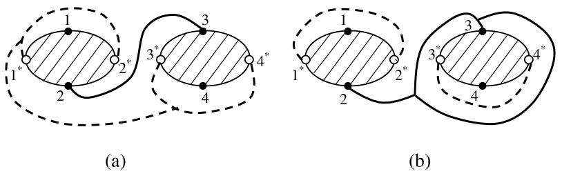
Figure 2: An $N=2$ example showing a given partition $X=(1)(23)(4)$ (solid line) can be the dual of two different partitions $Y_{1}$ and $Y_{2}$ (broken lines).
(a) $Y_{1}=(1^{*}2^{*}3^{*}4^{*})$, (b) $Y_{2}=(1^{*}2^{*})(3^{*}4^{*})$.

References

- [1] R. B. Potts, Some generalized order-disorder transformations, Proc. Camb. Philos. Soc. 48:106-109, (1952).
- [2] R. J. Baxter, Potts model at the critical temperature, J. Phys. C: Solid State Phys. 6:L445-448 (1973).
- [3] M. P. M. den Nijs, A relation between the temperature exponents of the 8-vertex and -state Potts model, J. Phys. A: Math. Gen. 12:1857-1868 (1979).
- [4] F. Y. Wu, The Potts model, Rev. Mod. Phys. 54:235-268 (1982).
- [5] F. Y. Wu, Potts model of magnetism, J. Appl. Phys. 55:2421-2426 (1984).
- [6] F. Y. Wu and Y. K. Wang, Duality transformation in a many component spin model, J. Math. Phys. 17:439-440 (1976).
- [7] P. G. Watson, Impurities and defects in Ising lattices, J. Phys. C: Solid State Phys. 1:575-581 (1968).
- [8] F. Y. Wu, Duality relation for Potts correlation functions, Phys. Lett. A 228:43-47 (1997).
- [9] F. Y. Wu and H. Y. Huang, Sum rule identities and the duality relation for the Potts -point boundary correlation functions, Phys. Rev. Lett. 79:4954-4957 (1997).
- [10] W. T. Lu and F. Y. Wu, On the duality relation for correlation functions of the Potts model, J. Phys. A: Math. Gen. 31:2823-2836 (1998).
- [11] C. King, 2D Potts model and annular partitions, J. Stat. Phys. 96:1071-1089 (1999).
- [12] F. Y. Wu, C. King, and W. T. Lu, On the rooted Tutte polynomial, Ann. Inst. Fourier, Grenoble 49:1103-1114 (1999).
- [13] C. M. Fortuin and P. W. Kasteleyn, On the random-cluster model I. Introduction and relation to other models, Physica 57:536:564 (1972).
- [14] I. J. van Lint and R. M. Wilson, A course in combinatorics (Cambridge University Press, Cambridge, 1992), p. 301.
- [15] R. P. Stanley, Enumerative Combinatorics Vol. 1 (Wadsworth and Brooks/Cole, Montery, California, 1986).
- [16] W. T. Tutte, A contribution to the theory of chromatic polynomials, Can. J. Math. 6:80-91 (1954).
- [17] W. T. Tutte, On dichromatic polynomials, J. Comb. Theory 2:301-320 (1967).