A microscopic mechanism for rejuvenation and memory effects in spin glasses

Abstract

Aging in spin glasses (and in some other systems) reveals astonishing effects of ‘rejuvenation and memory’ upon temperature changes. In this paper, we propose microscopic mechanisms (at the scale of spin-spin interactions) which can be at the origin of such phenomena. Firstly, we recall that, in a frustrated system, the effective average interaction between two spins may take different values (possibly with opposite signs) at different temperatures. We give simple examples of such situations, which we compute exactly. Such mechanisms can explain why new ordering processes (rejuvenation) seem to take place in spin glasses when the temperature is lowered. Secondly, we emphasize the fact that inhomogeneous interactions do naturally lead to a wide distribution of relaxation times for thermally activated flips. ‘Memory spots’ spontaneously appear, in the sense that the flipping time of some spin clusters becomes extremely long when the temperature is decreased. Such memory spots are capable of keeping the memory of previous ordering at a higher temperature while new ordering processes occur at a lower temperature. After a qualitative discussion of these mechanisms, we show in the numerical simulation of a simplified example that this may indeed work. Our conclusion is that certain chaos-like phenomena may show up spontaneously in any frustrated and inhomogeneous magnetic system, without impeding the occurrence of memory effects.

1 Introduction

The phenomena of slow dynamics in spin glasses, well known from the experiments in which the out-of-equilibrium effects are prominent Sitges ; Nordblad , have been these last years the subject of significant developments in theory Review , numerical simulations numerics , and also experiments on other glassy systems like e.g. polymers PMMA , supercooled liquids Nagel , dielectrics Levelut or gels gel . In the spin-glass phase, dynamical response functions evolve with time: this is the aging phenomenon, comparable with physical aging which has been widely studied in the rheology of glassy polymers Struik . Aging in spin glasses is evidenced in two general classes of ac and dc experiments. The starting point of aging is when the spin glass is cooled from above $T_{g}$ down to some temperature $T_{1}$ (usually $\sim 0.5-0.9T_{g}$).

In $dc$ experiments, e.g. zero-field cooled (‘ZFC’) procedure, the sample is cooled in zero field and kept at $T_{1}$ during a waiting time $t_{w}$. After $t_{w}$, a weak magnetic field is applied, and the slow increase of the magnetization is recorded as a function of time $t$. The response curves obtained depend on both independent time variables $t$ and $t_{w}$: they become slower and slower for increasing $t_{w}$. Similar results are obtained in the inverse procedure of cooling in a weak field and removing the field after $t_{w}$ (‘TRM’ procedure). In $ac$ experiments, equivalently, the response to a small oscillating field at frequency $\omega$ is found to relax slowly as the time $t$ from the quench elapses: here again two separate time scales ($\omega^{-1},t$) are involved Sitges . Such aging effects have now been clearly identified in numerical simulations of the three-dimensional Edward-Anderson model, and are also found in the analytical treatment of some mean-field models Review ; CuKu . They appear as a characteristic feature for the dynamics of randomly interacting objects.

The effect on aging of temperature changes has led to some non-trivial experimental results hierarki ; DTupps , recently emphasized as ‘memory and chaos’ or ‘memory and rejuvenation’ effects memchaos . Figure 1 (from Ref.VD ) shows the characteristic example of a negative temperature cycling experiment in ac mode. After a long aging stage at $T_{1}=0.72T_{g}$ (characterized by a downwards relaxation of $\chi"(\omega)$ by about 30%), a further cooling to $T_{2}=0.54T_{g}$ results in an apparent reinitialization of aging (‘rejuvenation’): $\chi"$ rises up to about the value that would be obtained after a direct quench, and a strong relaxation restarts. This observation contradicts the expectation from simple thermal slowing down, and suggests a possible indication of ‘chaos in temperature’ as proposed in Refs.bray ; domains . Following this ‘rejuvenation’ effect upon cooling, a completely different phenomenon is observed when re-heating from $T_{2}$ to $T_{1}$. The memory of aging at $T_{1}$ is retrieved, in the sense that $\chi"$ goes back to the value attained at $T_{1}$ before the temperature cycle, and relaxes in continuity with the previous part hierarki .

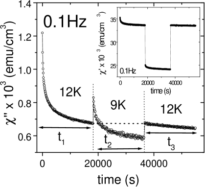
Figure 1: Effect on the $\chi^{\prime\prime}$ relaxation of a negative temperature cycling ($CdCr_{1.7}In_{0.3}S_{4}$ insulating spin glass with $T_{g}=16.7$K, frequency 0.1Hz, from Ref.VD ). Aging is mostly reinitialized during negative cycling (rejuvenation). The inset shows the $\chi^{\prime}$ behaviour during this procedure: the same effects are visible, but less clearly.

In the same way, a measurement of $\chi"(T)$ during continuous re-heating from low temperatures shows a ‘dip’ centered around $T_{1}$ memchaos . Astonishingly, it is even possible to ‘imprint’ and ‘read’ several memories at different temperatures, like in the example presented in Fig.2 VD . However, we shall mainly address here the question of the basic mechanisms underlying the observations of Fig.1. The multiple memories of Fig.2 will only be discussed as a possible extrapolation of our approach in Section 4.

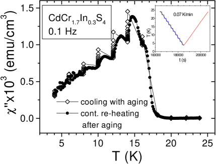
Figure 2: An example of multiple ‘rejuvenation and memory’ steps. The sample was cooled by 2K steps, with an aging time of 2000 sec at each step (open diamonds). Continuous re-heating at 0.001K/s (full circles) shows memory dips at each temperature of aging (from Ref.VD ).

A comprehensive description of this class of experiments in terms of a hierarchical organization of the metastable states as a function of temperature has been developed, and gives a satisfactory account of all results hierarki . This phenomenological picture has been made quantitative in models of random walk in a hierarchical set of traps BD ; Nemoto . However, the interpretation of the rejuvenation and memory effects in the real space of spins remains puzzling. From a comparison with aging in disordered ferromagnets, a scenario of pinned wall reconformations DWhierarchy has been proposed, in which the hierarchy of reconformation length scales is a real space transcription of the hierarchy of states ferro . But the exact nature of such walls in a spin glass remains mysterious martin . It is the purpose of the present paper to take a different point of view, and to consider microscopic and explicit mechanisms, at the scale of spin-spin interactions, which are possible candidates for being at the origin of these memory and rejuvenation effects.

On the basis of previous works on the reentrant phenomena in frustrated systemsREENT , we study example situations in which a slow evolution towards equilibrium at a certain temperature can be irrelevant to equilibration at another temperature (rejuvenation). On the other hand, the memory effect implies that spin rearrangements at one temperature do not irreversibly affect the structure grown at another temperature. This is the case for the mechanisms which will be considered here. Due to the inhomogeneity of the interactions, intricate developments of the spin-spin correlation take place, which should play an important role in the peculiar properties of spin glasses. Let us note that this intricate structure of the domains growing at different temperatures does not necessarily imply a fractal geometry.

In this paper, we limit ourselves to the study of examples of frustrated magnetic structures which, on the basis of phenomenological arguments, can be shown to reproduce the ‘single memory’ situation. The question of the extension of this basic mechanism to a double or multiple memory case, although conceivable (as discussed in Section 4), remains beyond the scope of the present paper.

2 Temperature dependent effective interactions and memory spots

In spin glasses, the ferromagnetic and antiferromagnetic bonds are randomly distributed. For statistical reasons, some regions of the lattice are highly frustrated, while others are less frustrated. The distribution of such regions is at the origin of complicated ordering processes, which are not as intuitively understandable as in the case of ferromagnets.

It has been early recognized Seiji that, in very simple frustrated systems of a few spins which can be analyzed exactly, the effective coupling constant between spins may behave strangely, such as changing of sign with temperature. This property, due to frustrated spin coupling, has been shown to generate reentrant phenomenaREENT . A similar idea has been more recently developed in the case of the Edwards-Anderson model Huse .

As an example, let us consider the simple 3-spin system pictured in Fig.3(a). If we consider the case where $J_{1}<0$ (antiferromagnetic) and $J_{2}>0$ (ferromagnetic), the spins $\sigma_{1}$ and $\sigma_{2}$ interact by frustrated bond structures. An effective coupling $J_{\rm eff}(T)$ between $\sigma_{1}$ and $\sigma_{2}$ can be defined by

$$e^{\beta J_{\rm eff}(T)\sigma_{1}\sigma_{2}}\propto\sum_{\sigma_{0}=\pm 1}e^{\beta J_{1}\sigma_{1}\sigma_{2}+\beta J_{2}(\sigma_{1}+\sigma_{2})\sigma_{0}}$$ (1)

where $\beta=1/k_{\rm B}T$, and $J_{\rm eff}(T)$ is explicitly given by

$$J_{\rm eff}(T)=J_{1}+{k_{\rm B}T\over 2}\ln[\cosh(2{J_{2}\over k_{\rm B}T})].$$ (2)

In the case $|J_{1}|<J_{2}$, $J_{\rm eff}$ changes sign as a function of temperature, as displayed in Fig. 3(b).

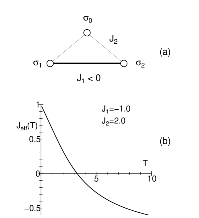
Figure 3: (a) An example of frustrated interaction. (b) The effective coupling constant $J_{\rm eff}(T)$ as a function of temperature.

From this simple example, it is clear that, due to frustration, ordering processes can change qualitatively with the temperature. We have listed in Appendix some realizations of the effective coupling in various frustrated situations. In the quoted examples, we see that the effective interactions may change with temperature in very different ways, even non-monotonically in some cases. If such bond configurations are randomly distributed in the lattice, it is clear that the equilibrium correlations at a given temperature do not coincide with those at other temperatures, a natural mechanism for rejuvenation effects. In a recent study of domain growth processes in a Mattis model YOSHINO , the consequences of bond changes on rejuvenation effects have been investigated (see a more detailed discussion in our last section). The microscopic mechanisms studied in our present paper can be considered as a possible explanation for the bond changes that have explicitly been assumed in YOSHINO .

Let us note that the effective couplings which are considered here correspond to a coarse-grained picture of the original lattice. Thus, the spins which are interacting via the effective bonds do in fact represent block spins, i.e. clusters of spins with less frustrated bond structures, as proposed in REENT . They are entities which already possess a significant entropy.

We expect the memory effect to be related to another characteristic of spin-glasses, which is that the relaxation times of spins distribute widely from spin to spin due to inhomogeneous interactionsTAKANO . As an example, let us consider the case depicted in Fig. 4, in which all couplings are ferromagnetic, one of them ($|J_{1}|$) being much larger than those of the surrounding bonds $J_{0}$ $(J_{1}\gg J_{0})$.

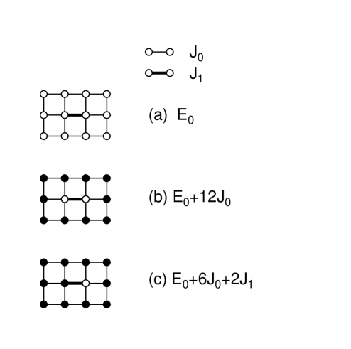
Figure 4: An example of memory spot ($J_{1}\gg 3J_{0}$). (a) stable state, (b) metastable state, and (c)unstable state. In order to relax from the metastable state (b) to the ground state (a), the system has to cross an energy barrier $\Delta E=2J_{1}-6J_{0}$ due to the intermediate state (c).

In Fig. 4(a), the ground state configuration with energy $E_{0}$ is shown; if all the external spins change sign, the two strongly coupled spins become metastable with energy $E_{0}+12J_{0}$, Fig. 4(b). In order to relax the two spins to the ground state, the system has to pass an intermediate state of higher energy $E_{0}+2J_{1}+6J_{0}$, Fig. 2(c). This corresponds to an energy barrier $\Delta E=2J_{1}-6J_{0}$. Thus, if $T\ll\Delta E$, it is difficult to flip the two spins, even if the surrounding spins are changed. The relaxation time is

$$\tau_{\rm mem}=\tau_{0}\exp\left({\Delta E\over T}\right),$$ (3)

where $\tau_{0}$ is a microscopic time; $\tau_{\rm mem}$ becomes suddenly long below a certain temperature. We expect that this kind of strongly coupled clusters are effectively realized in the less frustrated regions of a spin glass. Such clusters are distributed in the system, and can memorize a grown pattern of ordered configuration at a given temperature. We call them ‘memory spot’. When the temperature is lowered, the magnetizations of the stronger memory spots, which memorize the configurations at higher temperatures, are stable. In turn, when the temperature is raised, the memories for the lower temperatures are erased.

3 Rejuvenation and memory effects from basic mechanisms

Let us now summarize how a ‘rejuvenation and memory’ scenario can be built up with temperature dependent effective interactions and memory spots. Our qualitative discussion will be followed by the Monte-Carlo simulation of an example lattice.

If we quench the system from a high temperature to a certain value, say $T_{1}$, order corresponding to the minimization of the effective interaction energies at this temperature begins to grow. Let us consider the example sketched in Fig. 5(a). The fuzzy lines correspond to regions of high frustration, where the effective bonds at $T_{1}$ are weaker than in other parts and where in consequence domain walls are easily trapped. The ‘configurational domains’ delimited by these lines represent less frustrated regions.

Here we suppose that each domain has two degenerate minimum energy states, which are denoted by up and down arrows. We assume that the minimum energy state of the whole system with respect to the effective interactions at $T_{1}$ corresponds to all domain arrows pointing in the same direction. As we discuss later, the memory spots follow the direction of the domains in the time evolution at $T_{1}$, and record their direction at lower temperatures. In Fig. 5(a), the magnetization direction of the memory spots is shown by arrows for the equilibrium state.

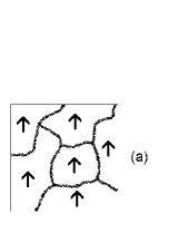
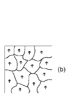
Figure 5: Schematic domain configurations after a waiting time (a) at $T_{1}$ and (b) at $T_{2}$. The domain boundaries, which consist of weaker bonds where the domain wall is easily trapped, are represented by lines. The memory spots (in (a) and (b)) are shown by arrows. The equilibrium spin correlations inside a domain can be rather general (Mattis model like); they do not coincide at both temperatures (the up direction of the arrows refers to the projection onto an arbitrary two-fold state).

In a short time $\tau_{\rm iD}$ after quenching, local order has been realized within each domain (low frustration). But no order between the domains has yet been established. That is, at this stage, the arrows of the domains are independently oriented. Then, waiting during $t_{w}$, correlations among the domains develop, with a flipping time scale $\tau_{\rm DD}$; meanwhile, $\chi"(\omega)$ decreases. The increase of the correlation length is very slow because as mentioned above the domain walls are naturally pinned at the boundaries slowDG .

We assume that the flipping time $\tau_{\rm mem}$ of the memory spot is less than the flipping time $\tau_{\rm DD}$ of the $T_{1}$ configurational domains. Hence the memory spots follow the direction of the domains, and record their direction as order among the domains develops. At lower temperatures, the magnetization of these memory spots will be frozen.

Then we change the temperature to $T_{2}<T_{1}$. Fig. 5(b) is a sketch of the configurational domains at $T_{2}$. Since the values of the effective bonds have changed, the grown domain structure grown at $T_{1}$ is just a random configuration for $T_{2}$ (rejuvenation). Thus new domains relevant to $T_{2}$ start growing, and $\chi"(\omega)$ rises back to a higher value.

Although the most part of the lattice has been rejuvenated, the memory spots remain stable because they consist of unfrustrated structures and $\tau_{\rm mem}$ increases rapidly as the temperature goes down. The structure at $T_{2}$ will be also recorded in smaller memory spots. In this way, the structure of order at each temperature can be recorded by memory spots of proper size, whose magnetization remains frozen at lower temperatures.

When re-heating to $T_{1}$, the order developed at $T_{2}$ in most of the lattice is now random with respect to order at $T_{1}$. However, in each $T_{1}$ configurational domain, the memory spot has memorized the previous direction of order. Therefore the domains tend to re-order according to their memorized direction, which rapidly reconstructs the configuration obtained at $T_{1}$ before the temperature cycle. Thus, in a very short time, $\chi"(\omega)$ decreases back to the value previously obtained (memory).

Let us now illustrate the above scenario by the numerical simulation of a simple model. We consider a lattice made of 5x5 times the unit clusters ($10\times 10$) shown in Fig. 6. The bonds $J_{1}$ and $J_{2}$ will mark the boundaries of the configurational domains at respectively $T_{1}$ and $T_{2}$. The memory spots are given by $J_{3}$. All other bonds are $J_{0}$. Table 1 displays the bond values at $T_{1}=2.0$ and $T_{2}=1.0$, the temperature variation being assumed to be due to the mechanisms described above.

Figure 6: Bond configuration (unit). The boundaries of the ‘configurational clusters’ will be given by the bold solid lines at $T=T_{1}$, and by the dotted lines at $T=T_{2}$

$T$ $J_{0}$ $J_{1}$ $J_{2}$ $J_{3}$ $T_{1}$= 2 1 1 0.5 3.2 $T_{2}$=1 $-1$ $-0.5$ $-1$ $3.2$

Table 1: Coupling constants for the bonds in Fig.6.

Obviously, from Table 1, the order is ferromagnetic at $T_{1}$ and (mostly) antiferromagnetic at $T_{2}$. We have chosen these two equilibrium configurations at $T_{1}$ and $T_{2}$ as simple examples; they might as well be any ground state choice of a Mattis model, as has been used in YOSHINO , as far as they are sufficiently different from each other.

Figure 7: (a) a configuration just after the short range order developed in each domain at $T_{1}$, (b) domain structures after a certain time at $T_{1}$, where correlation among the domains developed.

Figure 8: (a) an early stage configuration after the change of the temperature to $T_{2}<T_{1}$, (a’) configuration displayed in the antiferromagnetic gauge $\sigma_{i}\rightarrow\sigma_{i}\times\sigma^{0}_{i}$, where $\sigma^{0}_{i}$ gives the antiferromagnetic order, (b) developed new domain structure, at $T_{2}$, (b’) configuration displayed in the antiferromagnetic gauge and (c) recovery of the previous domain structure after the temperature comes back to $T_{1}$.

The initial configuration is completely random. In a short time $\tau_{\rm iD}$, order inside the domain develops, and the correlation length increases up to the size of the unit cluster ($\sim$ 10), as shown in Fig.7(a) for $t=10$MCS. In a second stage, order among the domains develops at the time scale $\tau_{\rm DD}\gg\tau_{\rm iD}$ (Fig.7(b) at $t=5000$MCS).

Then, at $t=5001$MCS, we change the temperature to $T_{2}$, which means changing the values of the effective couplings (Table 1). Antiferromagnetic order is now favoured. At $t=5010$MCS (Fig.8(a)), the new structure appears random (rejuvenation), but the memory spots are visible, clearly keeping track of previous ordering. In order to emphasize the new ordering process at $T_{2}$, we projected the configuration attained at $t=5010$MCS (Fig.8(a)) onto an antiferromagnetic ground state (‘transformed’ picture), as represented in Fig.8(a’). The new order among the new clusters has not yet grown. The $T_{1}$ memory spots can also be seen.

A new domain structure starts to develop within the time scale of $\tau_{\rm DD}(T_{2})$. Fig. 8(b) (direct) and 8(b’) (transformed) show the development at $t=7000$MCS of the new order at $T_{2}$ (the memory spots are still visible).

Then, at $t=7001$MCS, the temperature is increased back to its original value $T_{1}$. In a short time, most of the previous ordering is recovered, as can be seen from Fig.8(c) at $t=7100$MCS. The comparison of Fig.8(c) with Fig.7(b) shows that the memory of ordering at $T_{1}$ has actually survived to the rejuvenation process at $T_{2}$. The rapid re-ordering processes which occur immediately after re-heating to $T_{1}$ are likely to produce a short $\chi^{\prime\prime}$ ‘transient relaxation’, which has indeed been noted in some experiments hierarki ; DTupps .

4 Discussion

4.1 A plausible scenario for multiple memories ?

Beyond this simple example of rejuvenation and memory phenomena at two temperatures, the possibility of imprinting and reading multiple memories at several temperatures using the above mechanisms is a very incentive issue, even if it remains somewhat speculative. At different temperatures which are separated by a large enough interval $\Delta T$, we consider that the ordering patterns are decorrelated from each other, like different ground states in a Mattis model for different sets of bonds (for smaller $\Delta T$’s, it is clear that the ordering patterns will have similarities, and that the memory spots cannot fully work).

We suppose that the bond configuration of the memory spots is frozen at lower temperatures, as well as their orientation. Hence they memorize the signs of the local order (which is two-fold at each temperature). They will play the role of nucleation centers when the temperature is raised back.

The important point is that the memorized patterns do not correspond to ordering at other temperatures. At lower temperatures, the memory spots from higher temperatures are like frozen impurities. That is, the memory spots of a given pattern cannot act as nucleation centers for another pattern. This happens effectively in our numerical example (Fig.8): the ferromagnetically ordered spots do not have a significant influence on the antiferromagnetic order.

In the previous section, we chose ferromagnetic (F) and antiferromagnetic (AF) order as examples of two independent ordering patterns at $T_{1}$ and $T_{2}$. If we now consider a third temperature $T_{3}$ ($T_{3}<T_{2}<T_{1}$), the ordering pattern at $T_{3}$ must be independent of both F and AF, as mentioned above, and the memory spots for $T_{1}$ (F-ordered clusters) and for $T_{2}$ (AF-ordered clusters) will just be like frozen impurities. One may think of repeating this process in further and further cooling. How many ordering patterns can be treated as independent ones is an interesting problem, which is related to the question of pattern recognition in random networks, as studied in the Hopfield model network . In real systems, the number of spins is quite large, and it is not difficult to have several independent patterns; the present mechanism may thus work to memorize successive independent patterns at different temperatures. But the memory spots must be large enough to distinguish between different patterns, and also they have to be small compared with the ordering domains. In the simulation of the previous section, the ordering domains were $10\times 10$, and the memory spots were $2\times 3$. It is clear that the demonstration of multiple memories by simulations of our scenario will strongly be hindered by size limitations.

4.2 Rejuvenation effects and chaotic behaviour

The mechanism proposed here to be at the basis of rejuvenation effects is of ‘chaos-type’ bray ; domains , in the sense that it provides a microscopic basis for a ‘chaotic’ temperature dependence of the bonds. Memory is obtained due to the ‘memory spots’ which appear spontaneously in any inhomogeneous system. The question of ‘memory despite rejuvenation’ in domain growth processes has recently been discussed by Yoshino et al YOSHINO in an analytical and numerical study of the Mattis model. The Mattis model is purely random, but with no frustration, and the doubly degenerate ground state can be arbitrarily chosen by the set of the magnetic interactions. In YOSHINO , the bonds are changed ‘by hand’ from one set to another, and back (this is not far from the numerical example that we have presented here). A first order grows, say of A-type, then some other B-order develops, and coming back to A-bonds one may examine how far A-order has been preserved despite the rejuvenation caused by the growth of B-order. In the Mattis model, domain growth is a fast process because there is no frustration, so the memory of A-domain growth is rapidly erased by the growth of B-type domains. Due to its simplicity, the Mattis model is a useful ‘toy-model’ which even allows some analytic calculations YOSHINO . In a real (fully disordered) system, the growth of the correlation length is naturally much slower.

The study of the Mattis model YOSHINO shows that the large scale shape of the A-domains is preserved (memory), while the effect of rejuvenation can be seen as small scale ‘holes’ in the big A-domains. The same features can be observed in our numerical example, comparing Fig.7(b) and 8(c), but memory is here more robust thanks to the memory spots.

The fact that memory is preserved in large length scales, while rejuvenation occurs at short length scales, agrees well with the hierarchical sketch corresponding to the experiments hierarki . In contrast, the usual discussion of chaos in spin glasses bray ; domains is in terms of an overlap length beyond which the equilibrium correlations are re-shuffled by a temperature or bond change. In YOSHINO , and to a certain extent (apart from the memory spots) in the present numerical example, the overlap length between both considered states is zero, and rejuvenation and memory occur at respectively short and large length scales in a ‘hierarchical’ fashion.

The question of ‘chaos’ bray in the Edwards Anderson spin glass is rather puzzling. The spins in our present simplified picture can perhaps be compared with ‘block spins’ in the Edwards Anderson model, which have been shown in Huse to interact via effective bonds of temperature-dependent signs (in the same spirit as in REENT ; Seiji . It is intriguing that, in the present numerical simulations of the Edwards Anderson spin glass numerics , no clear rejuvenation and memory effects could be found in the dynamics (as well as no sign of chaos in the statics). In our present scenario, temperature dependent interactions and memory spots are obtained from simple bond arrangements. In a real spin glass, we argue that similar situations should statistically be realized due to the high number of random bonds. It is likely that this is not the case for numerical simulations, in which the number of spins may remain too small to allow the presence of such complicated structures as proposed here. On the other hand, the time scale of the simulations ($\sim 10^{5}$) is strongly limited compared to experiments ($\sim 10^{15}$), which benefit of very short microscopic ($\tau_{0}\sim 10^{-12}{\rm s}$) compared to laboratory ($t\sim 10^{0-5}{\rm s}$) time scales. Experiments Orbach and simulations numerics have shown that the spatial growth of the spin-spin correlation length $\xi$ is very slow ($\xi\sim(t/\tau_{0})^{0.15T/T_{g}}$), reaching hardly 5-10 lattice units in simulations. It is therefore very likely that Edwards Anderson simulations cannot spatially develop neither the kind of mechanisms that we have proposed here, nor the hierarchy of embedded length scales which should correspond to the hierarchical interpretation of the experiments hierarki ; DWhierarchy . In that case, the question of ‘chaos’ in the Edwards Anderson spin glass numerics might remain open for some time.

Finally, let us emphasize that, by discussing temperature dependent effective interactions as a possible origin of the rejuvenation effects found in experiments, we want to raise the question of a possible ‘classical’ origin of apparently ‘chaos-like’ phenomena. Indeed, an important feature of our present results (as well obtained in YOSHINO ) is that the ‘chaotic’ effect is mainly found at short distances (rejuvenation), while long distance correlations are preserved (memory). This is very similar to the theoretical case of an elastic line in presence of pinning disorder DWhierarchy , in which rejuvenation (and memory) effects can also be expected, due to the selection of smaller and smaller reconformation length scales as the temperature is lowered (see the discussion of experiments on spin glasses and disordered ferromagnets in ferro ). In such a system, when the temperature is decreased, the small length scales are driven out of equilibrium because of the classical thermal variation of the Boltzmann weights of configurations which were equivalent at a higher temperature, therefore new equilibration processes must restart.

5 Conclusion

In this paper, we have discussed some basic mechanisms which should be at play in frustrated (conflicting interactions) and inhomogeneous (interactions of various strengths) magnetic systems, and can thus be at the origin of the so-called ‘rejuvenation and memory’ phenomena.

Our first point is that, in the presence of frustration, the effective interaction between two spins (or domains) can take different values with even different sign at different temperatures (this same result explains some reentrance phenomena) REENT ; Seiji . As a second point, we have shown that the inhomogeneity of the interactions can by itself explain the memory effects, since regions with stronger interactions and less frustration will naturally remain frozen for very long times when the temperature is lowered. We have recalled simple examples which can be computed exactly.

Combining these two points, we have shown how rejuvenation and memory can take place in a simple numerical example. In the case of real spin glasses, many complicated bond structures exist, and are likely to correspond to different equilibrium spin structures for reasonably separate temperatures. Hence we expect that in a real spin glass the above scenario takes place ‘spontaneously’ between different temperatures.

In our numerical example, we considered that the system of spins as a whole was subjected to rejuvenation when the temperature is changed. That is, almost all bonds are changed by the temperature change. However, it is likely that only a part of the system rejuvenates. Multiple independent rejuvenation and memory stages, which take place at different temperatures (like in Fig.2), may then correspond to various embedded regions in the sample.

The ordering mechanisms that we have described, in which frustration and inhomogeneity play a major role, should be important ingredients for understanding the spin glass phenomena, at least at the mesoscopic scale, which is the most important for the observable slow dynamics. The extension of the present real space approach to a plain random bond distribution should offer a link with the phase space hierarchical picture, and clarify our understanding of the astonishing properties of spin glasses.

Acknowledgments

We are grateful to H. Yoshino, J.-Ph. Bouchaud, A. Lemaître, V. Dupuis, D. Hérisson, E. Bertin and J. Hammann for important discussions on various aspects of this work. We also want to thank the Monbusho grant (Grant-in-Aid from the Ministry of Education, Science, Sports and Culture in Japan), which made possible fruitful contacts and collaborations for several years.

6 Appendix: Temperature variations of effective coupling constants

In this appendix we show that the effective coupling between spins which interact by frustrated interactions can show a variety of temperature dependences. This idea has been discussed in previous papers Seiji , and shown to be at the origin of reentrant phase transitions REENT . Here we describe some fundamental mechanisms for various temperature dependences.

Let us consider the effective coupling constant between spins $\sigma_{1}$ and $\sigma_{2}$ related by a linear chain with $n$ bonds like in Fig. 9(a). We assume, for simplicity, that all the bonds are the same and equal to $J$. We define the effective coupling $K_{\rm eff}$ by the correlation function of $\sigma_{1}$ and $\sigma_{2}$:

$$\langle\sigma_{1}\sigma_{2}\rangle=\tanh K_{\rm eff}.$$ (4)

Tracing out the intermediate spins (${\rm s}_{1}$,$\cdots$ ${\rm s}_{n-1}$), we obtain

$$K_{\rm eff}(n,T,J)={1\over 2}\left({1+\tanh^{n}\beta J\over 1-\tanh^{n}\beta J}\right)$$ (5)

where $\beta=1/k_{\rm B}T$. The effective interaction $J_{\rm eff}=K_{\rm eff}/\beta$ varies with temperature.

Let us now consider two chains of different lengths $n$ and $m$, like in Fig. 9(b). The effective coupling between the spins $\sigma_{1}$ and $\sigma_{2}$ is the sum of the contributions of the two chains:

$$K_{\rm eff1}(n,m,T,J,J^{\prime})=K_{\rm eff}(n,T,J)+K_{\rm eff}(m,T,J^{\prime})\ .$$ (6)

If the signs of the two contributions are different, these interactions suffer frustration. In Fig.10(a), we show the temperature dependence of $K_{\rm eff1}$ for $(n=10,J)$ and $(m=11,J^{\prime}=-J)$ as a function of $T/J$. We see that the effective coupling stays constant at low temperatures. By the relation (4), the fact that the effective coupling stays constant means that the spin correlation function does not develop up to unity. That is, the spins do not align completely even at low temperatures. Here , we used the same amplitudes for $J$ and $J^{\prime}$ in order to cancel the coupling at low temperatures. But of course we can use different ones. Indeed, the example given in Section 3 corresponds to $K_{\rm eff1}(1,2,T,J,-2J)$, where the effective coupling changes sign.

Because of the additive nature of the effective couplings Eq.(6), we can arrange various temperature dependences making use of the step-function like dependence of $K_{\rm eff1}$. For example, we can make an effective bond which is relevant only in a limited temperature range, by combining $K_{\rm eff1}(n,n+1,T,J_{1},-J_{1})$ and $K_{\rm eff1}(n,n+1,T,J_{2},-J_{2})$ as

$$K_{\rm eff2}(n,T,J1,J2)=K_{\rm eff1}(n,n+1,T,J_{1},-J_{1})$$

$$+K_{\rm eff1}(n,n+1,T,J_{2},-J_{2})\ .$$ (7)

Fig. 10(b) shows $K_{\rm eff2}$ in the case $n=10$, $J_{1}=J$ and $J_{2}=-1.2J$.

An example of a further complicated case is shown in Fig. 10(c), the effective coupling of which is made of two contributions of the type of (7):

$$K_{\rm eff3}(T)=K_{\rm eff2}(n,T,J_{1},-1.2J_{1})$$

$$+K_{\rm eff2}(n,T,-2J_{1},2.4J^{\prime}_{1})\ .$$ (8)

The examples in this appendix show that a remarkably wide variety of temperature dependences can be obtained in this way.

Figure 9: Spins $\sigma_{1}$ and $\sigma_{2}$ coupled by : (a) a chain of $n$ spins ($s_{1},\cdots,s_{n}$), (b) two chains of $n$ and $m$ spins ($s_{1},\cdots,s_{n}$, and $s_{1},\cdots,s_{m}$).

Figure 10: (a) Temperature dependence of $K_{\rm eff1}$ for the case of $n=10$ and $m=11$ ($J=-J^{\prime})$. (b) Temperature dependence of $K_{\rm eff2}$ for the case of $n=10$ $J_{1}=J$ and $J_{2}=-1.2J$. (c) Temperature dependence of $K_{\rm eff3}$ for the case of $K_{\rm eff3}(T)=K_{\rm eff2}(n,T,J_{1},-1.2J_{1})$ $+K_{\rm eff2}(n,T,-2J_{1},2.4J^{\prime}_{1})$.

References

- (1) E. Vincent, J. Hammann, M. Ocio, J.-P. Bouchaud, L.F. Cugliandolo, in Complex Behaviour of Glassy Systems, Springer Verlag Lecture Notes in Physics Vol.492, M. Rubi Editor, 1997, pp.184-219, e-print cond-mat/9607224, and refs. therein.
- (2) P. Nordblad and P. Svedlindh, in ‘Spin-glasses and Random Fields’, A. P. Young edt. (World Scientific, 1998), pp.1-28, and refs. therein.
- (3) For a review of different theoretical models leading to aging, in particular mean-field models, see: J.-P. Bouchaud, L. F. Cugliandolo, J. Kurchan, M. Mézard, in ‘Spin-glasses and Random Fields’, A. P. Young edt. (World Scientific, 1998), pp.161-224, e-print cond-mat/9702070.
- (4) H. Rieger, Ann Rev. of Comp. Phys. II, ed. D. Stauffer (World Scientific, Singapore, 1995); E. Marinari, G. Parisi, F. Ritort and J. J. Ruiz-Lorenzo, Phys. Rev Lett. 76, 843 (1996); T. Komori, H. Yoshino and H. Takayama, J. Phys. Soc. Jpn. 68, (1999) 3387; M. Picco, F. Ricci-Tersenghi, F. Ritort, e-print cond-mat/0005541.
- (5) L. Bellon, S. Ciliberto and C. Laroche, Europhys. Lett. 51, 551 (2000).
- (6) L. Leheny and S.R. Nagel, Phys. Rev. B 57, 5154 (1998).
- (7) P. Doussineau, T. de Lacerda-Arôso and A. Levelut, Europhys. Lett. 46, 401 (1999).
- (8) D. Bonn, H. Tanaka, G. Wegdam, H. Kellay and J. Meunier, Europhys. Lett. 45, 52 (1998); L. Cipelletti, S. Manley, R.C. Ball and D.A. Weitz, Phys. Rev. Lett. 84, 2275 (2000).
- (9) L. C. E. Struik, ‘Physical aging in Amorphous Polymers and Other Materials’, Elsevier Scient. Pub. Co., Amsterdam (1978).
- (10) L.F. Cugliandolo and J. Kurchan, J. Phys. A: Math. Gen. 27, 5749 (1994), and Phys. Rev. B 60, 922 (1999).
- (11) Ph. Refregier, E. Vincent, J. Hammann and M. Ocio, J. Phys. France 48, 1533 (1987); E. Vincent, J.-P. Bouchaud, J. Hammann and F. Lefloch, Phil. Mag. B 71, 489 (1995).
- (12) P. Granberg, L. Lundgren and P. Nordblad, J. Magn. Magn. Mater. 92, 228 (1990); P. Granberg, L. Sandlund, P. Nordblad, P. Svedlindh and L. Lundgren, Phys. Rev. B 38, 7097 (1988).
- (13) K. Jonason, E. Vincent, J. Hammann, J.-P. Bouchaud and P. Nordblad, Phys. Rev. Lett. 31, 3243 (1998); K. Jonason, P. Nordblad, E. Vincent, J. Hammann and J.-P. Bouchaud, Europ. Phys. Jour. B 13, 99 (2000).
- (14) V. Dupuis, PhD thesis, in progress.
- (15) A.J. Bray and M.A. Moore, Phys. Rev. Lett.58 (1987) 57.
- (16) D. S. Fisher and D. A. Huse, Phys. Rev. B 38, 373 and 386 (1988); G. J. M Koper and H. J. Hilhorst, J. Phys. France 49, 429 (1988).
- (17) J.-P. Bouchaud and D.S. Dean, J. Phys. I France 5, 265 (1995); J.-P. Bouchaud, in “Proceedings of the Fifty Third Scottish Universities Summer School in Physics. Soft and Fragile Matter: Nonequilibrium Dynamics, Metastability and Flow (St Andrews NATO School)”, pp. 285-304, Cates M.E. and Evans M.R. eds. (Bristol and Philadelphia 2000), e-print cond-mat/9910387.
- (18) M. Sasaki and K. Nemoto, J. Phys. Soc. Jap. 69, 2283 (2000).
- (19) L. Balents, J.-P. Bouchaud, M. Mézard, J. Physique I 6, 1007 (1996); see also Review .
- (20) E. Vincent, V. Dupuis, M. Alba, J. Hammann and J.-P. Bouchaud, Europhys. Lett. 50, 674 (2000).
- (21) J. Houdayer, O. C. Martin, Europhys. Lett. 49, 794 (2000).
- (22) H. Kitatani, S. Miyashita and M. Suzuki, J. Phys. Soc. Jpn. 55 (1986) 865.
- (23) S. Miyashita, Prog. Theor. Phys. 69, (1983) 714.
- (24) D.A. Huse and L.F. Ko, Phys. Rev. B 56, 14597 (1997).
- (25) H. Yoshino, A. Lemaître and J.-P. Bouchaud, accepted for publication in EPJ B (2001), preprint cond-mat/0009152.
- (26) H. Takano and S. Miyashita, J. Phys. Soc. Jpn. 64, 423 and 3688 (1995).
- (27) D.A. Huse and C.L. Henley, Phys. Rev. Lett. 54, 2708 (1985); T. Kawasaki and S. Miyashita, Progr. Theor. Phys. 89, 1167 (1993).
- (28) J. J. Hopfield, Proc. Nat. Acad. Sci. USA 79, 2554 (1982), and 81, 3088 (1984). D. J. Amit, Modeling Brain Function, Cambridge, 1989. E. Domany, J. L. van Hermann and K. Schulten, Model of Neural Networks III, Springer 1995.
- (29) Y.G. Joh, R. Orbach, G.G. Wood, J. Hammann and E. Vincent, Phys. Rev. Lett. 82, 438-441 (1999).