I Introduction
The microscopic derivation of the effective time-dependent Ginzburg-Landau
(GL) theory continues to attract attention since an early paper
by Abrahams and Tsuneto Abrahams . Whereas the static GL potential
was derived Gor'kov from the microscopic BCS theory soon after its
introduction, the time-dependent GL theory is still a subject of interest
(see Aitchison.1997 ; Aitchison for a review on the problem’s history).
One of the reasons for this is the presence of Landau damping terms
in the effective action. For -wave superconductivity these terms
are singular at the origin of energy-momentum space, and consequently
they cannot be expanded as a Taylor series about the origin.
In other words, these terms do not have a well-defined expansion
in terms of space and time derivatives of the ordering field and therefore
they cannot be represented as a part of a local Lagrangian.
We recall that at and for the static (time-independent) case
the Landau damping vanishes, so that either at one still has
a local well-defined time-dependent GL theory or for
the familiar static GL theory exists. It is known, however,
that for -wave superconductivity even though the Landau terms
do exist, they appear to be small compared to the main terms of
the effective action in the large temperature region
Aitchison , where is the superconducting transition temperature.
This is evidently related to the fact that only
thermally excited quasiparticles contribute to the Landau damping.
The number of such quasiparticles at low temperatures appears to be a small
fraction of the total charge carriers number in the -wave
superconductor due to the nonzero superconducting gap
which opens over all directions on the Fermi surface.
For a -wave superconductor there are four Dirac points (nodes)
where the superconducting gap becomes zero
on the Fermi surface.
The presence of the nodes increases significantly the number of the
thermally excited quasiparticles at given temperature comparing to
the -wave case. Therefore one can expect that the Landau damping
should be stronger for superconductors with a -wave gap which
is commonly accepted to be the case of high-temperature
superconductors (HTSC) d-wave . Moreover, it is believed that
at temperatures ,these quasiparticles are reasonably
well described by the Landau quasiparticles, even though such an
approach fails in these materials at higher energies Lee .
This is the reason why one can hope that a generalization of the BCS-like
approach Aitchison for the 2D -wave superconductivity may be
relevant to the description of the low-temperature time-dependent
GL theory in HTSC.
In this work we derive such a theory from a microscopical model with
-wave pairing extending the approach of Aitchison
developed for -wave superconductivity. As known from Abrahams
the physical origin of the Landau damping is a scattering of the
thermally excited quasiparticles (“normal” fluid) with group
velocity from the excitations of phase
(or -) quantums. Such
conversion occurs only if the Čerenkov condition,
for the energy and momentum
of the -excitation is satisfied. This phenomenon
in superconductivity is also called Landau damping since its
equivalent in the plasma theory was originally obtained by Landau
(see e.g. Sitenko ).
To emphasize the difference between the Landau damping for - and
-wave pairing, we also derive for the comparison the corresponding terms
for a 2D -wave superconductor. In addition we compare 2D expressions
obtained here with the 3D -wave case studied in Aitchison .
The collective phase oscillations in charged -wave superconductor
for clean and dirty cases were recently studied in Takada .
Due to the complexity of the corresponding equations they were solved
numerically, neglecting damping of the phase excitations. Thus our fully
analytical treatment can be very useful for further studies
of the phase excitations. We also mention a recent paper
Randeria.action where the effective action for the phase mode in
the -wave superconductor was obtained using the cumulant expansion.
The Landau terms were neglected in Randeria.action , but the effect
of Coulomb interaction was taken into account.
Our main results can be summarized as follows.
1. We find that the main physical difference between the -
and -wave cases is related to the fact that for -wave
superconductivity the direction of the quasiparticle group
velocity ( is the quasiparticle dispersion law) does not
coincide with the Fermi velocity
Lee ; Carbotte and a gap velocity
also enters into the Čerenkov condition along with .
2. We show that the intensity of the Landau damping has a linear
temperature dependence at low with a coefficient expressed
in terms of the anisotropy of
the Dirac spectrum .
Here () are the projections of the quasiparticle momentum
on the directions perpendicular (parallel) to the Fermi surface.
The parameters , and proved to be very
convenient both in the theory, for example, of the transport phenomena
Lee , ultrasonic attenuation Carbotte in -wave superconductors
and for the analysis of various experiments Chiao .
3. We find that the Landau damping is sensitive to the direction
of the phason momentum. In particular, for a given node the Landau
damping is possible only if the components of the phason momentum
(which are defined exactly as the components
of the quasiparticle momentum above) satisfy the
condition .
4. We derive a simple approximate representation for the Landau
damping terms which can be useful for further studies of the
-wave superconductors.
5. We derive an approximate expression for the propagator of the
Bogolyubov-Anderson mode which includes the Landau damping.
6. Concerning the mathematical formalism used in the paper,
we adapt the bilocal Hubbard-Stratonovich field method of Kleinert
to the -wave pairing. Additionally we adjust the technique of the
derivative expansion for the “phase only” action
(see Aitchison and Refs. therein) for the model with the
tight-binding spectrum.
The paper is organized as follows:
In Section II we present our model and write down
the partition function using a bilocal Hubbard-Stratonovich field.
In Section III, we introduce the modulus-phase variables and
represent the effective “phase only” action as an infinite series.
It appears that the low-energy phase dynamics is contained in the first two
terms which are evaluated, respectively,
in Sections IV and V with some
details considered in Appendix A.
The effective Lagrangians for the - and -wave cases without the Landau
damping are discussed in Section VI.
In Section VII we derive the damping terms
and in detail compare - and -wave cases. The approximate forms
of the effective action and - propagator are considered in
Section VIII. Section IX
presents our conclusions and comments on a possible experimental
observation of the phase excitations.
II Model
Let us consider the following action
|
|
|
(1) |
where the Hamiltonian is
|
|
|
(2) |
Here is a fermion field with the spin
, ,
is the imaginary time and
is an attractive potential.
For the sake of the simplicity we consider the dispersion law,
for a model on a
square lattice with the constant including the nearest-neighbor
hopping only. This, however, is not an essential restriction because the
final results for the -wave case will be formulated in terms of
the non-interacting Fermi velocity
and the gap velocity
defined in the Introduction.
The bilocal Hubbard-Stratonovich fields
and
(see e.g. Kleinert ) can be
utilized to study the model (1), (2)
|
|
|
(3) |
On the right hand side, is understood as
numeric division, no matrix inversion being implied. The hermitian conjugate of
includes the transpose in the
functional sense, i.e. .
Thus in the Nambu variables
|
|
|
(4) |
the partition function can be written as
|
|
|
(5) |
where
and , are Pauli matrices.
In general an electron-electron attraction on the nearest-neighbor
lattice sites can be considered (see, for example, Nikolaev ; Meintrup ).
The momentum representation for this interaction contain in the
pairing channel extended -, - and even -wave pairing terms:
|
|
|
(6) |
Motivating by
HTSC we consider here -wave pairing only, so
that for the Fourier transform of the pairing potential
we use
|
|
|
(7) |
As was mentioned in Introduction, we will compare the main results
for the -wave case with the simplest 2D continuum -wave
pairing model (see e.g. Gusynin.JETP1 and the
review Loktev.review ) which has a quadratic dispersion
law and a local attraction
.
III The Effective Action
While for the model with the local four-fermion attraction
Aitchison ; Gusynin.JETP1
the modulus-phase
variables could be introduced exactly, one should apply an additional
approximation for treating the present model.
Let us split the charged fermi-fields and
in (5) into the neutral
fermi-field foot1
and charged Bose-field
|
|
|
(8) |
It is clear that the terms containing in
(5) can be treated similarly to the old model and the
problem arises when one deals with the Hubbard-Stratonovich field. To consider
this field we introduce the relative
and center of mass coordinates .
Now we can introduce the modulus-phase representation for the
Hubbard-Stratonovich field
|
|
|
(9) |
where is the modulus of the Hubbard-Stratonovich
field and is its phase.
Assuming that the global phase
varies slowly over distances on the order of a Cooper pair size and thus
is not sensitive to the inner pair structure described by the relative
variable , we can rewrite (9) as
|
|
|
(10) |
The approximation we made writing Eq. (10) is in fact
equivalent to the Born-Oppenheimer approximation Thouless.1993
which allows one to separate the dynamics of the Cooper pair formation
described by the relative coordinate in
from the motion of the superconducting condensate
described by the center mass coordinate in
.
If the condensate motion
is slow enough this separation becomes
possible because the dynamics of the Cooper pair formation
can always follow the motion of the condensate.
Using the lattice language one can also say about
(10) that the bond phase
is replaced by the site phase Tesanovic .
Applying the transformations (10) and
(8) to the terms with the Hubbard-Stratonovich field
in (3) we obtain (the imaginary time is omitted)
|
|
|
(11) |
where we used the assumption (or
hydrodynamical, long wavelength approximation, see
Palo.1999 ) that varies slowly,
.
Here is the coherence length which for the BCS theory coincides
with an average pair size.
Then the partition function in the modulus-phase variables is
|
|
|
(12) |
where the effective potential
|
|
|
(13) |
with
|
|
|
(14) |
|
|
|
(15) |
|
|
|
(16) |
Thus the gauge transformation (8)
resulted in the separation of the dependences on and ,
viz. is present only in . The similar method of
the derivative expansion was used before in Aitchison.1995 ; Aitchison .
As pointed out in Aitchison the method allows to
maintain explicitly the Galilean invariance
(the Landau terms break it) and the continuity equation, while the
expansion used recently
in Takada demands the additional
enforcement of the conservation laws Kulik .
Since the low-energy dynamics in the phase in which
is determined by the long-wavelength fluctuations
of , only the lowest order derivatives of the phase
such as , and
need be retained in what follows. However, to take into account
the tight-binding electron spectrum the operators
and must be kept. Thus in we have omitted
higher order terms in , but in order to keep all relevant
terms in the expansion of the necessary resummation
was done Sharapov:1998:PC . One can easily see that for the quadratic
dispersion law ,
and , so that Eq. (16)
reduces to the known expression from Aitchison.1995 ; Aitchison .
Thus we arrive at the one-loop effective action
|
|
|
(17) |
where
|
|
|
(18) |
and
|
|
|
(19) |
Deriving the “phase only” action for the -wave model it was possible to
use Loktev.review .
The -wave case is more complicated because one should keep the dependence
on the relative coordinate,
which is related to
the nontrivial pairing.
The dependences of the gap on , and follow
from the extremum condition for the mean-field
() potential
which results in the usual BCS gap equation.
For the -wave pairing potential (7)
one obtains
|
|
|
(20) |
where is the gap amplitude. In our case there is no need
to solve the gap equation and express in terms of
, and since in what follows we will use ,
or more precisely the velocity , as the input
parameters and will be interested in the low temperature
() regime.
Thus assuming that
does not depend on one obtains for
the frequency-momentum representation of (15)
|
|
|
(21) |
where is given by (20) and
is fermionic (odd) Matsubara frequency.
The phase dynamics is contained in the kinetic part
of the effective action which only involves the single degree of freedom
. As discussed in Aitchison , it is enough to restrict
ourselves to terms with in the infinite series in
(18) since at this would give
the right answer for a local time-dependent GL functional which
involves the derivatives not higher than and
.
IV The First Order Term of the Effective Action and
the Nodal Approximation
In this section we calculate the first () term of the sum appearing
in (18):
|
|
|
(22) |
Summing over Matsubara frequencies, one obtains
|
|
|
(23) |
with ,
and
|
|
|
(24) |
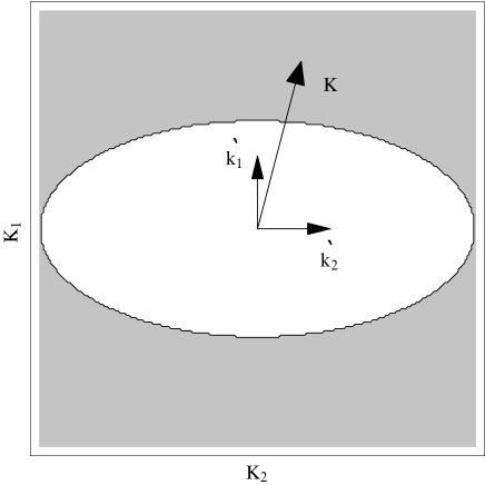
For
linearizing the quasiparticle spectrum about the nodes and defining a
coordinate system at each node with
() perpendicular (parallel) to the Fermi surface, we can
replace the momentum integration in (23) by an integral
over the -space area surrounding each node Lee .
If we further define a
scaled momentum we can let
|
|
|
(25) |
where , and . Note that for the particular square lattice model used above
those velocities are and respectively.
Using (25) one can express Eq. (23)
in terms of and
|
|
|
(26) |
where
|
|
|
(27) |
is the density of carriers.
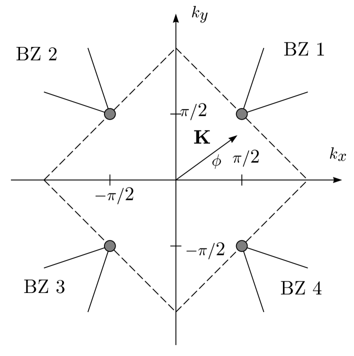
We note that due to the slow convergence of the integrand in
(26) the final expression depends explicitly on the value
of the momentum cutoff which was defined in Lee in such a way
that the area of the new integration region over 4 Brillouin sub-zones
(see Fig. 1) is the same as that of the original
Brillouin zone. Going from Eq. (23) to
(26) we essentially replace the averaging over the
true Fermi surface of the system by the averaging over 4 nodal sub-zones.
The validity of this approximation can only be justified if the
corresponding integrals contain the derivative of the Fermi distribution
which is highly peaked in the vicinity of the nodes.
This appears to be the case of the temperature dependent parts
of the phase stiffness , compressibility and the
Landau damping terms. For the zero temperature values
and the nodal approximation is not well justified.
However, as we show in Sec. VI, this approximation can
be justified a forteriory for their ratio (see Fig. 2)
which determines the velocity of the Bogolyubov-Anderson-Goldstone mode.
Finally, we stress that after approximation is used, it is impossible to
recover the -wave limit by putting .
V The Second Order Term of the Effective Action
Let us evaluate the trace of the second term
in expansion (18):
|
|
|
(28) |
Substituting (16) into (28) we obtain that
|
|
|
(29) |
where using we denoted symbolically that the
corresponding term of (28) is either diagonal
(i.e. its frequency-momentum representation contains
or ) as
|
|
|
(30) |
|
|
|
(31) |
or mixed
|
|
|
(32) |
In (30) - (32)
we introduced the following short-hand notations
|
|
|
(33) |
More generally, we can rewrite Eqs. (31)
and (32) as follows
|
|
|
(34) |
|
|
|
(35) |
where
|
|
|
(36) |
,
we used the approximation and took into account that
.
It is convenient to introduce here
|
|
|
(37) |
which would allow to rewrite (30)
in the same fashion as (34).
As one could notice the product of the Fermi velocities enters
Eq. (34) via (36).
There is nothing surprising in this
fact since this piece of the effective action is related to the paramagnetic
current correlator
Randeria.action
and in its turn the current operator, contains the Fermi
velocity .
We will return to this point considering the Landau
term which originates from (34), so that here we
note only that the current correlator term along with
the diamagnetic term in Eq. (22)
form together the mean-field phase stiffness.
The matrix traces and the corresponding expressions
for are calculated in Appendix A. Although
the expressions for them are rather lengthy they have a clear
physical interpretation which is also discussed in the Appendix.
VI The effective Lagrangian at without the Landau terms
The contribution of the first order term to the effective action is given in
(26). Concerning the second order term, we note that
when the Landau terms are neglected it is enough to
set inside in (30),
(34) and
(35). To be more precise,
the Landau terms arise from the second line of Eqs. (74)
and (75) which contains “dangerous” denominators
. One can
however notice that the second line of Eq. (74) leads also to the
regular terms which are proportional to the derivative .
These lead to the second term in the square brackets
in (38) and the whole expression (39)
shown below.
For the -wave superconductivity Gusynin.JETP1 ; Aitchison in the
temperature region these terms are very small
compared to the main terms.
Although the contribution from these terms is still local, their
presence breaks the Galilean invariance Aitchison .
This is the reason why it was more natural for Aitchison to treat them
along with “true” Landau terms since they also originate
from the same denominators of the second line of (74) as was
mentioned above.
For the -wave superconductivity this splitting, however, appears
to be rather artificial since these terms are not small even for low
temperatures due to the presence of the nodal quasiparticles, so here
we will consider all regular terms.
For the regular terms from the second order term we obtain a local
effective action, involving time and space derivatives of :
|
|
|
(38) |
|
|
|
(39) |
and the mixed term (35)
does not contribute to the regular part within the used
approximation, since .
Evaluating (38) and (39)
we performed the analytical continuation back to the real continuous frequencies, so that is the real
time.
Using the nodal expansion (25) to calculate
(38), (39) and adding (26)
we finally obtain the regular effective Lagrangian,
such that
for and ignoring the Landau terms:
|
|
|
(40) |
where the phase stiffness and
compressibility are
|
|
|
(41) |
The linear time derivative term in
(40) is important for the description of vortex
dynamics (see Randeria.action and Refs. therein), but we
omit it in what follows.
We stress that the second, temperature dependent term in
follows from Eq. (39) which contains the derivative
of the Fermi distribution, . Its presence, as we mentioned
in Sec. IV, makes the nodal approximation valid
Lee .
Since we consider only the low temperature
region, we restrict ourselves by the values
and at , so that all temperature
dependences appear to be linear. For higher temperatures
it is necessary to take into account that and
are in fact decreasing functions of .
It is useful to compare the stiffness and compressibility
from (41) with those parameters derived
in Gusynin.JETP1 for the continuum 2D model
with -wave pairing:
|
|
|
(42) |
First of all one can see that for low temperatures the superfluid
stiffness in (42) does not contain any term which
goes to zero more slowly
than , while (41)
has a term proportional to . The origin of this difference is
well-known and related to the presence of the nodal quasiparticles.
Secondly, we can compare the values of the zero temperature superfluid
stiffness which for the continuum translationally invariant system has to
be equal to , so that all carriers participate
in the superfluid ground state Leggett . Since the presence of
a lattice evidently breaks the continuum
translational invariance the superfluid
density at in the case of (41) is less than
, as can be readily seen from (23).
Finally, since we consider here a neutral system it has the
Berezinskii-Kosterlitz-Thouless (BKT) collective mode
foot2 , with .
One can see that for the continuum -wave case and
|
|
|
(43) |
for the -wave model on lattice at .
Eq. (43) gives rather simple approximate expression
for the BKT mode velocity for the lattice model of
-wave superconductor. Comparing in Fig. 2 the results
obtained for using Eq. (43) with the numerical
computation without the nodal approximation, we can see that
that even being very simple Eq. (43) predicts the correct
behavior of .
Following Randeria.action we estimate the upper
values for the frequency in (38) and the momentum
in (39). The “phase-only” effective action
is appropriate for phase distortions whose energy is smaller than
the condensation energy, , where
is the density of states. For the -wave case (42)
this leads to the following restrictions: ,
and for the -wave case
(41): ,
,
where is the anisotropy of the Dirac spectrum defined
in Introduction.
VII The imaginary part of the Landau terms for 2D -wave
and -wave cases
The key values which are necessary for evaluation of the Landau terms are the
differences and .
Expanding in ,
|
|
|
(44) |
where the group velocity is given by
|
|
|
(45) |
It is obvious that due to the gap -dependence
Eq. (44) differs from the -wave case Aitchison , where the difference is simply
|
|
|
(46) |
It is convenient to rewrite (44) and
(45) in terms of the nodal approximation described after
Eq. (25). In the vicinity of one of the nodes we have
|
|
|
(47) |
where the momentum of -particle was also
expressed in the nodal coordinate system
, , so that
, and
.
(We denoted the components of as to
make them different from the node label used in what follows.)
The corresponding
substitution in the integrals over reads
similarly to Eq. (25)
|
|
|
(48) |
where is evidently related to the maximal value of
discussed at the end of Sec. VI.
Finally, we can approximate the difference
as
|
|
|
(49) |
Having the differences (47) and (49)
we can now derive the imaginary part for the Landau terms.
In the subsequent subsections we consider all three
terms of Eq. (29) for -wave pairing
and compare them with their -wave counterparts.
We would like to note that the Landau terms have also
the real part which for the 3D -wave case was consider
in detail in Aitchison . This real part consists of
regular and irregular terms. The regular term was already taken into
account in Sec. VI and the irregular term
is not considered in this paper.
VII.1 term
Let us consider firstly the contribution from
(see
Eqs. (30) and (74) for ), which
after the analytical continuation takes the form
|
|
|
(50) |
Here is the step function and we used the integral
|
|
|
(51) |
Integrating over we had to take into account that there are two
points where -function contributes into the integral:
,
and
,
.
As we can see from the first equality in
(50) the imaginary
part develops when .
This condition was interpreted in Abrahams as the “Čerenkov”
irradiation (absorption) condition for the process:
“thermally excited -fluctuation quantum (phason) + quasiparticle
phason + quasiparticle” (or
phason being absorbed and scattering thermally excited quasiparticles).
As was discussed in Lee , since definite energy
is carried by the quasiparticles, this process is defined by their
group velocity
Abrahams as well as thermal and spin currents.
It is in fact a coincidence that for the -wave superconductor the directions
of and are the same, so that for the 2D -wave
superconductor using (46) instead of
(44) and (45)
one can obtain
|
|
|
(52) |
where following Aitchison we used the notations
and .
Comparing (52) with the 3D case Aitchison
(in the notations of Aitchison the term we consider
is related to the sum )
one can notice that the only difference between the corresponding
expressions is in the square root in the denominator of
(52). It obviously originates from
the different measures for the angular integration in 2D and 3D where
the extra is present. Comparing also
(50) and (52)
one can see that their main analytical structure appears to be
the same, viz. for the -wave case
and for the -wave case, so that the momentum
variables and do not appear in the numerator.
We note that the calculation of the ultrasonic attenuation
in -wave superconductors results in the
expression
|
|
|
(53) |
which has the same structure as (50).
This can be easily seen if one takes into account that
for ultrasound frequency range
, so that
the corresponding terms from Eq. (50)
can be simplified as follows
|
|
|
(54) |
leading to Eq. (53). This the reason why in the limit
the angular dependence of the Landau damping
(50) which we consider in
Sec. VIII would appear to be the same as
the angular dependence of the ultrasonic attenuation Carbotte .
VII.2 term
The contribution from
(see Eqs. (34) and (74) for )
can be treated in the same manner
|
|
|
(55) |
and for the -wave case
|
|
|
(56) |
Let us now compare the expressions (55) and
(56). Evidently their analytical structure
is different since for the -wave case we have again that it is
proportional to , while for -wave pairing
enters the numerator, so that the main structure
(excluding the measure of integration over and the square
root in the denominator) is .
This difference originates from the angular integration in
(55) and (56)
which is performed using the -function. Since the arguments
of the -function for the - and -wave cases
are different we have obtained two different answers.
Indeed, for the -wave case the argument is proportional to
that coincides with the product
outside the -function.
(see Sec. V after Eq. (34),
where the origin of the term
is discussed), so that the angular integration
removes from the numerator. The -wave case appears to be different
since we have inside the -function
and outside, so that the angular integration leaves in the numerator.
Despite the fact that looks substantially less
singular than , the first expression still remains
nonanalytical near because it is expressed in terms
of the coordinate representation of which is the
non-local operator .
Thus physically the difference between the analytical form of the Landau
damping in - and -wave superconductors originates from
the -dependence of the gap
which in its turn makes the direction of the quasiparticle group velocity
different from the Fermi velocity .
The last velocity, however, still enters the numerator of
(55) since, as was already mentioned in
Sec. V, it originates from the current-current
correlator. The electrical current is proportional to
, not because quasiparticles carry definite
energy and spin, but do not carry definite charge.
Therefore, the specific form of the Landau damping terms
in a -wave superconductor has the same physical origin as the source
of the extra terms in the thermal and spin conductivities Lee
which are related to the presence in both
and components.
The -wave Landau damping (56) itself
can be again related to the 3D case Aitchison , where
it is expressed via the difference .
VII.3
term
Finally we consider the contribution from
(see Eqs. (35) and (75)):
|
|
|
(57) |
and for the -wave case
|
|
|
(58) |
Once again the difference between - and -wave cases is related to the
different directions of and . Since this
time we had
outside the -function, we
could not get as in
Eq. (55) and obtained again
as in Eq. (50).
Furthermore, because we have instead
of as in Eq. (50)
we got only got only
(compare with the square brackets in Eq. (50))
which after multiplying by gives the final
result . It is interesting to note that the mixed
term for - (see Eq.(57))
and -wave (see Eq.(58))
has the opposite with respect to other terms sign. This means
that the mixed term describes the energy transfer from the
quasiparticles to the phase excitations. It turns out, however,
that the whole sum (59) of the Landau damping terms
has the sign which corresponds to the phason damping.
(We stress that the different sign in front of all final -wave
expressions and their -wave counterparts are due to the explicit
presence of the derivative of the Fermi distribution, which is negative,
in the former expression.)
VII.4 Final expression for the Landau damping term in the -wave case
Since the Landau damping terms for -wave pairing all are
, we can combine (52),
(56) and
(58):
|
|
|
(59) |
This expression coincides with the function
introduced in Aitchison except for the above mentioned
difference between angular integration in 2D and 3D.
Thus the simultaneous derivation of the - and -wave
cases allowed us to be sure that all relevant terms
were included and to see explicitly why the corresponding
- and -wave terms behave so differently.
VII.5 Temperature and energy-momenta dependences of Landau Damping
We now compare the conditions on the momenta and energies for
the existence of the nonzero Landau terms in - and -wave
cases and the temperature dependences of these terms.
As one can see from Eqs. (50),
(55) and (57)
for a given node the imaginary parts
develop when
(or ).
Thus in contrast to the -wave case when the imaginary part is nonzero
for all directions of the phason momentum satisfying the
condition
(or , where is defined after
Eq. (52)), for the -wave it is
sensitive to the direction of the phason momenta as shown in Fig. 3.
As we will discuss in Sec. VIII for HTSC
, so that the directional anisotropy of the Landau
damping becomes very strong. Indeed as can be seen from Fig. 3
for and the Landau
damping would exist only in a narrow region of the momenta directions.
Furthermore, if the projection of the phason momentum
is not exactly zero (),
the condition can be well
replaced by .
We will discuss the validity of this approximation in
Sec. VIII.
It is important to stress that the sharp directional
dependence discussed here is not related to the nodal approximation and
follows only from the gap anisotropy and the fact that the difference
of the Fermi distribution functions (49)
which is present in Eqs. (50),
(55) and (57)
has a very sharp -dependence, so that in principle
unbounded (for example, for the model
with the quadratic dispersion law Aitchison )
functions and in
the corresponding integrals were replaced by their values at the
Fermi surface.
The final expressions (50),
(55) and (57)
for the -wave case are in fact
simpler than their -wave counterparts, (52),
(56) and
(58) (or the final expression
(59))
because the latter expressions
still have one integration which depends on the ratio
via the -function. Thus if , only
large contribute into the corresponding integrals.
This circumstance
and the opening of an isotropic gap
make the contribution from the Landau terms very small comparing to the
main terms. For -wave pairing a relative contribution of
the Landau terms does not depend on the ratio
via integration,
so that all frequencies and momenta satisfying the conditions
imposed by the -functions in (50)
and (55) have the same temperature dependent
weight.
As in the case with the superfluid density the temperature dependence
of the Landau terms is linear in , but while the superfluid
density is nonzero at , there is no Landau damping at .
The linear dependence and the absence of damping at
are obviously related to the fact that for -wave
pairing there are only four gapless points on the Fermi surface.
It is known, for example, that for a normal (nonsuperconducting) system
the Lindhard function (or polarization bubble)
|
|
|
(60) |
has a nonzero imaginary part even at Schrieffer if
the Fermi surface remains ungapped since the derivative of the Fermi
distribution at becomes singular on the entire
Fermi surface (or line in 2D).
Finally, we note that there is also imaginary contribution
even from the first, “superfluid” term in (74) for .
As we already mentioned, this term involves pair breaking
which for -wave pairing has the threshold energy, .
For -wave pairing this energy is zero for
due to the presence of nodes. Nevertheless, if a
finite energy is necessary to create these excitations
and the imaginary contribution is nonzero only for .
Besides the analytical structure of this term is regular and
it has a higher order than the terms considered here.
Thus this term appears to be less important than
the Landau terms we just considered.
VIII The Approximate Form of the Effective Action and
-propagator
Whereas the local nodal coordinate systems are convenient to
write down the corresponding contributions from each node, the final result
should be presented in the global or laboratory
coordinate system . It is
convenient to measure the angle from the vector ,
so that corresponds to the corner of the Fermi surface
(see Fig. 1) and the first node is at . Thus the
transformations from the global coordinate system into the local system
related to the -th node are
|
|
|
(61) |
The estimates of Chiao show that in YBCO
and in BSCCO (see Table 1).
Thus we can also use the inequality
in what follows. First of all this inequality implies that for
-th node we may assume that
|
|
|
(62) |
This approximation is, of course, valid only if is not
parallel to the Fermi surface ().
We note that this direction which is “dangerous” for -th node
is the nodal direction for the neighboring nodes. The size
of the “dangerous” direction where Eq. (62) becomes
invalid can be estimated from the condition
which gives .
Since Eq. (62) is in fact well
justified outside the nodal regions.
Using Eq. (62)
we can also rewrite the discussed in Sec. VII.5
inequality imposed by -functions which
define the region where the Čerenkov condition can be satisfied
as
|
|
|
(63) |
One can easily see that the condition (63)
is in fact equivalent to the condition
we already mentioned.
The effective action (18) in the momentum
representation in the global coordinate system can be written as
|
|
|
(64) |
with the regular (compare with Eqs. (40) and
(41))
|
|
|
(65) |
and Landau, , parts.
It is possible to
write down substituting
(61) directly into (50)
and (55), but to have a more
transparent expression we would like to consider a more simple case
.
This condition becomes equivalent to due to the
presence of -functions in (50),
(55) and (57)
which are cutting out the forbidden domains with .
Physically, the condition is
relevant if one, for instance, estimates the Landau damping for
the BKT mode (43)
because it follows from (43) that
.
Thus we obtain
|
|
|
(66) |
where
|
|
|
(67) |
|
|
|
(68) |
and
|
|
|
(69) |
The functions , and are obtained from
(50), (55) and
(57),
respectively. Deriving (67) - (69) we used the
the assumption replacing the square roots in
(50), (55) and
(57) by 1. Furthermore,
we kept only from (50).
Nevertheless, we kept the -functions which are present
in (50), (55) and
(57) because they are
essential in imposing the condition .
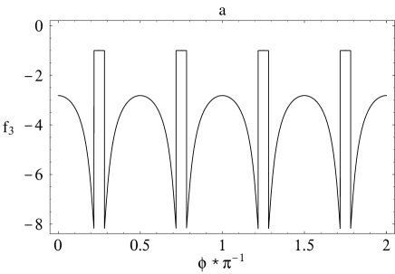
In Figs. 4 (a), 5 (a) and 6 (a)
we show the functions , and which describe the intensity
of Landau damping ( and for the term
and for the term , respectively) as a function
of the direction in the plane. Although the functions and
describe the directional dependence for the same
term, we do not combine these functions into the single function
because they originate from the different expressions.
(We recall that originates from Eq. (50)
and originates from Eq. (57),
respectively.)
For the comparison in Figs. 4 (b), 5 (b)
and 6 (b) we show the directional dependences
calculated by the direct substitution of Eq. (61) into
Eqs. (50), (55)
and (57) without making the
approximations we just described. As one can see, the approximate
representation (66), (67) - (69)
despite its relatively simple form (we have used only the terms
and ) gives reasonably good
expression for the Landau damping terms. The biggest discrepancies
are seen between Fig. 4 (a) and Fig. 4 (b)
because more approximations were made to obtain term.
As we mentioned in Sec. VII, the angular dependence
described by (see Fig. 4 (a))
coincides with the angular dependence of the
ultrasonic attenuation Carbotte in the limit .
Indeed the -functions from (67) disappear when
and Eq. (67) reduces to the
corresponding equation from Carbotte .
We stress also
that the analytical structure of the damping terms in
(66) appears to be quite different
from the dissipation introduced in
Benfatto.dissipation into the “phase only” action basing
on the low frequency conductivity measurements.
Since and terms are odd functions of the frequency ,
they integrate to zero in .
Nevertheless, the damping terms are manifest in the equation
of motion and in the propagator of the BKT mode which is
considered below.
Comparing Figs. 4, 5 and 6, one can see that
the functions and have more pronounced angular dependence
than . Although as we explained above, the contribution from a
given node is zero if for some the condition
(63) is not satisfied, this
condition can still simultaneously be satisfied for the neighboring
nodes, so that the sum over all nodes in – is not necessarily
zero.
We note also that by the absolute value both (or ) and
terms are practically the same. This can be easily seen if we rewrite,
for example, term as
|
|
|
(70) |
where writing the last identity we explicitly used the ratio
for the BKT mode at given above.
In such a way following Aitchison we can write an approximate
propagator of the BKT mode near as
|
|
|
(71) |
with
|
|
|
(72) |
As discussed in Aitchison Eq. (71) has
the form of a bosonic propagator with damping and its line-width
has an explicit dependence. In contrast to
the -wave case, the width depends not only on the absolute value of
, but also on the direction of .
The angular dependence for
is shown in Fig. 7.
Despite a simple form of the propagator (71),
the corresponding effective wave operator (the transform of
to space and time)
has a nonlocal form in coordinate space due to the presence
of the damping term which depends Aitchison on .
Comparing the second term in parentheses of (71) with
the damping term one can see that they have the same order of magnitude
showing that even for the low temperature region the Landau damping becomes
important and its magnitude is comparable with term which describes the
linear low temperature decrease in the superfluid stiffness.
We stress also the difference between the Landau damping representation
in Eqs. (71) and (66).
While the propagator (71) relies on the particular
dispersion law for the BKT mode with the approximate
given by Eq. (43), our Eq. (66)
along with Eqs. (67) - (69) present a rather general
representation for the Landau damping terms derivation of which
did not rely on any particular dispersion law for the phase
excitations. Thus it can be, in principle, used to describe the damping
of the plasmons in charged superconductor. The only assumption we made is that
, which was used to derive more simple and transparent
representation for the Landau damping. For the more general case
one should use the results from Sec. VII.
IX Concluding Remarks
It is very important to note that the collective phase excitations
described by the propagator similar to (71)
can and have indeed been studied experimentally. Indeed
the measurements of the order parameter
dynamical structure factor in the dirty Al films allowed
to extract the dispersion relation of the corresponding Carlson-Goldman
mode and to investigate its temperature dependence Goldman .
It is important to stress that since the real systems are
charged this mode appears to be different from
the sound-like Bogolyubov-Anderson mode which exists in a
neutral superfluid Fermi liquid. However, as discussed in
Kulik (see also Takada and Refs. therein)
the discovery of Carlson-Goldman collective mode Goldman
overcame the widespread opinion that the Bogolyubov-Anderson
collective oscillations predicted for a neutral superfluid should
be forced to the frequencies on the order of the plasma frequency.
It appears that if under certain conditions the frequency of the phase
excitations is sufficiently low, the normal electron fluid may screen
completely the associated electric field, thereby making the theory of
uncharged superconductor applicable Brieskorn . The conditions
for screening and occurrence of the Carlson-Goldman mode in -wave
superconductors are favorable only if the systems are dirty
(to suppress the Landau damping) and Kulik .
As recently claimed in Takada in -wave superconductors
the conditions appear to much less strict, so that the Carlson-Goldman
mode may be observed in the clean systems for down to .
Now there are some new questions which would be interesting to address
from both experimental and theoretical points of view.
First of all, there is a general question whether the Carlson-Goldman
mode which is the equivalent of the Goldstone mode for the charged
system can be observed experimentally. There are also a lot
of theoretical questions which study would make this kind of experiment
possible. Leaving aside the specific of the Carlson-Goldman mode
studied in Takada we mention some of them which are directly
related to the present work.
1. The Carlson-Goldman experiment Goldman measures
so called dynamical structure factor. This factor has a peak
associated with the phase excitations the width of which is primarily
controlled by the Landau damping. Therefore our result that
the intensity of Landau damping has a strong directional
dependence should be taken into account in the calculation of
the structure factor. In particular, the lowest for the observation
of the Carlson-Goldman mode temperature in Takada
is obtained for the nodal direction. As can be seen from, for example,
Fig.4 and 5, the corresponding
Landau damping terms become maximal in the vicinity
of this direction which should likely result in widening
of the corresponding peak. If this widening is too big that the peak
may become unobservable, this would again suggest that
the dirty samples should be used for the experiment.
2. Taking into account the lattice effects and the dominance
of the nodal excitations we have obtained that the velocity
of the phase excitations at is given by
(see Eq. (43) and the
discussion after Eq. (23)).
This expression appears to be quite different from the well-known continuum
result, .
The estimates of the velocities and
obtained from the values and
Chiao are presented in Table 1.
It is seen from these estimates that the difference between
the description proceeding from continuum and lattice models can be
quite different. However the estimates of the minimal
for the observation of the Carlson-Goldman mode temperature in Takada
are based on the continuum expression .
Thus it would be interesting to reconsider these estimates
for the lattice case.
3. Finally, as pointed out in Randeria.action
if the plasmon is at finite frequency at , the Landau
damping does not occur since when is finite and
it is impossible to satisfy Čerenkov condition discussed
above. However, a very small value of the plasma frequency in HTSC
suggests that the Landau damping may still be relevant when
is nonzero and the Čerenkov condition can be satisfied.
Thus the corresponding damping terms should be included in the
“phase only” actions which are used to describe plasma excitations
in -wave superconductors. Predicted anisotropy of the Landau
damping would result in the damping anisotropy for the plasma
excitations.
To summarize, we have considered the “phase only” effective action
for so called neutral (or uncharged) fermionic
superfluid with - and -wave pairing in 2D. When the damping terms
are included into this action, it turns out non-local in coordinate
space and its analytical structure for the -wave case is very
different from the -wave case.
To consider a charged superfluid it is necessary to combine the approaches
used in the present paper and in Randeria.action ; Takada to
consider the Landau damping in the presence of Coulomb interaction.
Appendix A
Substituting (21) into (30) and
(34), using the definitions for
and and evaluating the matrix traces for the
diagonal terms we obtain
|
|
|
(73) |
Performing in (73) the summation over Matsubara frequencies and
simplifying the result we arrive at
|
|
|
(74) |
where , and . The second
term in Eq. (74) can be further simplified if one notices that the term
with transforms into the term when . Note that the
terms do coincide with the corresponding terms in Aitchison .
For the mixed term (35) one obtains
|
|
|
(75) |
To get the last identity we again replaced
and took into account that also changes sign
under this transformation.
One can also check that .
Eq. (75) is also in agreement with the corresponding term
in Aitchison denoted as .
The first and second terms in (74) and (75) have a
clear physical interpretation Schrieffer .
The first term gives the contribution
from “superfluid” electrons. The second term gives the contribution
of the thermally excited quasiparticles (i.e. “normal” fluid component).
The essential physical difference between the two terms is that
the superfluid term involves creation of two quasiparticles,
with the minimum excitation energy in the -wave case being .
(For the -wave case the minimum energy turns out to be zero in the
four nodal points, see the discussion at the end of
Sec. VII.)
On the other hand, the normal fluid term
involves scattering of the quasiparticles already present
and the excitation energy in this case can be arbitrary small,
as in the normal metal, independently whether we are in the vicinity of
the node or not. Of course, the number of the
quasiparticles participating in this scattering depends on
the value of the gap and drastically increases if the gap is equal
to zero in some points.
As we shall see, the Landau damping terms originate from the second,
normal fluid term. Note that our Eqs. (74) and (75)
(as well as Eqs. (30),
(34) and
(35))
are suitable for studying both - and -wave cases.