Against Temperature Chaos in Naive TAP Equations

Abstract

We study the temperature structure of the naive TAP equations by mean of a recursive algorithm. The problem of the chaos in temperature is addressed using the notion of the temperature evolution of equilibrium states. The lowest free energy states show relevant correlations with the ground state, and a careful finite size analysis indicates that these correlations are not finite size effects, ruling out the possibility of chaos in temperature even in the thermodynamic limit. The correlations of the equilibrium states with respect to the ground state are investigated. The performance of a new heuristic algorithm for the search of ground states is also discussed.

I Introduction

The mean-field theory of spin glasses (SG) based on the Sherrington-Kirkpatrik (SK) model has revealed very interesting properties of its low-temperature phase. Among them there are a rugged free-energy landscape with many metastable states, universality of the probability distribution function of the overlap between states, and their ultrametric organization [4]. These properties are common to various randomly frustrated systems, but the full analytic control is formulated mostly for the SK model.

The first attempt toward a Curie-Weiss theory of the SG phase has been done within the TAP theory [5], in which a set of non-linear equations for the mean site magnetizations $\{m_{i}\}$ has been introduced much in the same spirit of the mean-field equations for ordinary ferromagnets. Such a set of equations has been analytically investigated in [6], where it has been found that the number of minima increases exponentially with the system size (precisely as $\exp(\alpha(T)N)$, being $\alpha(T)$ some temperature dependent $O(1)$ constant and $N$ the number of spins), and that there exists a temperature dependent free energy threshold above which the solutions of the TAP equation are uncorrelated (i.e. their mutual overlap is zero in the limit of $N\rightarrow\infty$). However a number of questions about the detailed structure of the metastable states of the SK model still remains unanswered.

A direct numerical solution of the TAP equations is difficult because of the so called Onsager reaction term (we will discuss about it in the following), which introduces a portion of the configuration space in which the equations themselves lose their validity [6, 7]. Here we will study a simplified version of TAP equations, obtained from the original ones dropping the numerically dangerous Onsager reaction term. This new set of equations is known as the naive mean-field (NMF) equations, and they become the exact mean-field equations for a generalized SK model [8]. This model turns out to have strikingly similar SG properties to the original SK model [9], capturing all the complexities of the SG phase, but with mean-field equations open to easier numerical integration. This model, as well as the original SK model, displays Replica Symmetry Breaking.

The main focus of this work has been the analysis of the organization of the equilibrium states at different temperatures. The motivation that led us to this problem is that while, at least at the mean-field level, it is well known that below $T_{C}$ states at the same temperature in the SG phase are non-trivially correlated, very little is known about the correlations between states at different temperatures, despite intense theoretical and numerical efforts on this subject in the last fifteen years.

The hypothesis of the chaos in temperature can be very simply stated in terms of absence of correlations between states at different temperatures. It was originally introduced as a constitutive ingredient of the phenomenological droplet theory [11] in order to take into account the absence of strong cooling rate dependence experimentally not observed in real spin glasses [12, 13]: the approach to equilibrium of a given observable after cooling from the high temperature to a working temperature $T_{W}<T_{C}$ does not depend on the thermal history of the experimental sample, but only on the time spent at the last temperature $T_{W}$ [14]. The puzzle becomes more intricated once we turn our attention to the memory effects observed in temperature cycling experiments [14]: the state reached by a system at a given temperature below $T_{C}$ is recovered after a negative temperature cycle. The memory effects are manifestly contradicting the chaotic scenario suggested by the cooling rate insensitivity, giving rise at the same time to a number of theoretical explanations mostly focused on real space point of view [15, 16]. Let us stress a possible source of misunderstanding: in [12] it was related temperature chaos with bond-chaos, i.e. perturbation on the systems induced by infinitesimal changes in the quenched disorder. While the latter it has been clearly shown to be present [17], we believe to be able to demonstrate in what follows that the two forms of chaos are different and that, at least at the mean field level, no temperature chaos is present.

On the pure theoretical side, even at the mean-field level, the situation is still far from being satisfactory. Chaos in temperature was first advocated in an unpublished work of Sompolinsky, then reconsidered negatively in [18] at zero-loop order (i.e. for the infinite range limit of the theory), then again supported in [19] at one-loop order (i.e. for the short range case). Lastly we point out the work of Franz et al. [20] where, by means of the coupled real replicas method [21], they supported the presence of chaos. This approach was recently reconsidered in [22], where it was demonstrated that taking into account higher order perturbation terms, there is no chaos in temperature.

On the numerical side, clues of chaos in temperature for short range spin glass model were discussed in [23, 24, 25], while our results are in substantial agreement with the simulations presented in [26] where it was observed that the overlap correlation length in 3D Edwards-Anderson model (EA) is a monotonically increasing length scale with respect of the aging time, and with the more recent simulations of the SK model and the 3D Edwards-Anderson model presented in [27].

In this work we carried out a careful numerical analysis of the solutions of the naive TAP equations. We solved these equations by using a recursive algorithm in the spirit of [9, 10]. We managed to give a coherent description of the temperature structure of the solutions, that we have classified into two families: solutions appearing just below the critical temperature which display a bifurcation scenario as the temperature is decreased, and a huge number of solutions appearing well below the critical temperature. We have addressed our investigation on the changes in temperature of the free energy landscape by operatively defining the temperature evolution of a generic equilibrium state. This allowed us for the analysis of the correlations between the ground state and its temperature evolved state: the obtained results suggest a temperature smoothly varying free energy landscape, and consequently a non chaotic scenario. Exploiting this temperature evolution technique we have also been able to characterize the nature of the first solutions just below $T_{C}$: it turns out that these solution are highly correlated with the ground state, suggesting a scenario in which the first minima appearing just below the paramagnetic phase are also the deepest ones throughout the whole SG phase. Let us stress that our findings are strengthened by a careful finite size scaling analysis that rules out the possibility that our results are finite size effects. The interpretation of the temperature structure of the equilibrium phase space has suggested to us the implementation of a heuristic algorithm for the search of the ground states that gives an approximate value for the ground state energy density which is always less than $1\%$ higher than the true ground state.

The paper is organized as follows. In Sec. II we will introduce both the model and the numerical method. In Sec. III we will discuss the nature of the tree of solutions of the naive TAP equations in terms of their free energy landscape. In Sec. IV we will discuss the temperature organization of the equilibrium states. We will show in terms of free energy landscape that the minimum originating from the ground state shifts smoothly with respect of temperature changes with no sign of temperature chaos. In Sec. V we will discuss the performance of a new heuristic algorithm for the search of the ground states. In Sec. VI we will briefly summarize our findings and comment on further developments.

II Model and numerical methods

The main difference between the replica method and the TAP approach is that while in the former we can only calculate observables averaged over the disorder probability distribution function, using the latter we can gain information about single sample quantities, eventually averaging the results over the disorder at a later stage of the calculation. A rigorous derivation of the self-consistency equations for the magnetization of the SK model gives [4, 5]:

$$m_{i}=\tanh\left[\beta\left(\sum_{j=1}^{N}J_{ij}m_{j}+h_{i}-\beta\sum_{j=1}^{N}J^{2}_{ij}(1-m_{j}^{2})m_{i}\right)\right]\,.$$ (1)

This formula is a system of $N$ coupled non-linear equations for the local magnetizations $m_{i}\equiv\langle s_{i}\rangle$. The physical interpretation of the terms involved in the TAP equations is rather simple: the first two terms inside the hyperbolic tangent in the r.h.s of (1) are the usual mean-field terms of ordinary ferromagnets, while the last one is the Onsager reaction term, which is a measure of the contribution to the internal field acting on the site $i$ coming from the magnetization $m_{i}$ itself. Such a term is relevant in the case of the SK model because the generic coupling $J_{ij}\propto N^{-1/2}$, while for a ferromagnetic theory the coupling is $O(1/N)$ (the free energy must be proportional to $N$), so that, at the mean-field level, this term is never taken into account. In the paramagnetic phase and for small values of $\tau=T_{C}-T$ the local magnetizations are expected to behave as $m_{i}=\tau^{1/2}+O(\tau)$, so that the Onsager term drops to zero as $\tau^{3/2}$ apart from a constant term whose main effect is to shift the critical temperature. In the low temperature phase ($\beta\rightarrow\infty$) a detailed replica calculation shows that $q_{EA}\equiv 1/N\sum m_{i}^{2}=1-O(\beta^{-2})$ (at least for the lowest energy states), so that $\beta(1-q_{EA})=O(\beta^{-1})$ and again the Onsager term drops. The analytical calculation presented in [9] and numerically confirmed in [28], yields a value of $T_{C}=2$ for the critical temperature, where it has to be noticed that the critical temperature for the SK model (i.e. for the complete TAP equation (1)) is $T_{C}=1$.

In the following we will set to zero the Onsager term and the extern magnetic field $h_{i}$, and we will use random symmetric Gaussian couplings of zero mean and variance $1/N$. Under these assumptions we can rewrite (1) as follows:

$$m_{i}=\tanh\left(\beta\sum_{j=1}^{N}J_{ij}m_{j}\right)\,.$$ (2)

As we have mentioned above in the low temperature phase (2) has a lot of solutions. We shall label them with $m_{i}^{\alpha}$, and we shall use in general the superscript $\alpha$ to denote quantities such as the free energy $F^{\alpha}$ related to the corresponding solution:

$$F^{\alpha}=E^{\alpha}-\frac{S^{\alpha}}{\beta}\,,$$ (3)

where the internal energy $E^{\alpha}$ and the entropy $S^{\alpha}$ are given by:

$$E^{\alpha} = -\sum_{1\leq i<j\leq N}J_{ij}m_{i}^{\alpha}m_{j}^{\alpha}$$ (4)

$$S^{\alpha} = -\frac{1}{2}\sum_{i=1}^{N}\left[(1+m_{i}^{\alpha})\ln\left(\frac{1+m_{i}^{\alpha}}{2}\right)+(1-m_{i}^{\alpha})\ln\left(\frac{1-m_{i}^{\alpha}}{2}\right)\right]\,.$$ (5)

In the following we will mainly deal with densities of thermodynamic potentials. We shall adopt for these quantities the standard lowercase notation $f^{\alpha},e^{\alpha},s^{\alpha}$.

Let us stress that, at least for the naive TAP equations, it is easy to demonstrate that the critical temperature $T_{C}$ is self-averaging observing that in the paramagnetic phase (i.e. high temperature) the equation (2) can be rewritten as $m_{i}=\beta\sum_{k}J_{ij}m_{j}$. The transition temperature $T_{C}$ in this contest is the temperature where the paramagnetic solution $\{m_{i}=0\}$ becomes unstable. From random matrix theory [29] it is known that this temperature corresponds with the higher positive eigenvalue (which is $2$) and moreover such an eigenvalue turns out to be self-averaging.

Denoting with $N_{S}(T)$ the number of solutions of (2) at temperature $T$, the link between the TAP formalism and the single sample mean-field partition function is given by

$$Z_{J}=\sum_{\alpha=1}^{N_{S}(T)}e^{-\beta F^{\alpha}}\,,$$ (6)

which encodes the intuitive idea of Boltzmann weighted sum over the solutions [30]. The internal density of energy can be expressed, according to (6), as:

$$e=-\frac{1}{V}\frac{\partial\ln(Z_{J})}{\partial\beta}=\frac{1}{V}\sum_{\alpha=1}^{N_{S}(T)}\frac{e^{-\beta F^{\alpha}}}{Z_{J}}\frac{\partial}{\partial\beta}(\beta F^{\alpha})=\sum_{\alpha=1}^{N_{S}(T)}e^{\alpha}w^{\alpha}\,,$$ (7)

where we defined the weights $w^{\alpha}\equiv e^{-\beta F^{\alpha}}/Z_{J}$, and we exploited the stationarity conditions $\partial_{m_{i}}F=0$, which are the mean-field equations (2).

In order to solve (2) we used a recursion algorithm in the spirit of [28, 31]. We start by generating a random initial configuration $m_{i}^{(0)}$ taken from a flat probability distribution function with support in $[-1,1]$, and then we start the recursion:

$$m_{i}^{(t+1)}=\tanh\left(\beta\sum_{j=1}^{N}J_{ij}m_{j}^{(t)}\right)\,.$$ (8)

The algorithm stops when $\sum|m_{i}^{(t+1)}-m_{i}^{(t)}|<10^{-6}$. The algorithm was implemented in double precision, in order to avoid rounding problems. We also checked that the state obtained by the converging recursion is effectively a solution of (2) by direct inspection. In the following we will assume that two solution $\{m_{i}^{\alpha}\},\{m_{i}^{\beta}\}$ of (2) have to be considered as different whenever $\sum|m_{i}^{\alpha}-m_{i}^{\beta}|>10^{-2}$. Given this requirement we have found no difficulty in distinguishing solutions. We have also checked that the results do not change when more stringent bounds are adopted. Note that the maximum volume reached in our simulations was $N=200$.

The exhaustive enumeration of the solutions at a given temperature was achieved following this simple procedure: each solution obtained by the iteration is accumulated into a stack if it is different from all the other solutions already accumulated. Each solution is also labelled with the number of times that it has been found by the recursion. The search stops after all solutions in the stack have been found at least $10$ times. We also tried to increase this number but we did not find any increase in the total number of the solutions, at least within the volume accessible for exhaustive enumerations, which for us is $N\leq 28$ for the whole SG phase, and $N\leq 200$ down to $T=T_{C}/2=1$. We insist here on the strict requirement of exhaustive enumeration, by checking that each solution has the magnetic reversal counterpart. It is in fact obvious that if $\{\hat{m}_{i}$} is a solution of (2), also $\{-\hat{m}_{i}\}$ will be a solution with the same free energy as a consequence of the overall $Z_{2}$ symmetry of the model.

III The tree of the solutions

The detailed knowledge of the temperature scenario of the states of the mean-field SG phase is lacking so far. The main problem is that while the more complete description available today is within the replica approach, this task is very complex from the analytic point of view. The TAP formalism bypasses this fundamental difficulty allowing us for a complete description of the single sample Boltzmann states, at least at a numerical level.

We have already mentioned the exponential number of solution of both TAP equations [5], and the naive SK mean-field model [9]. It would be interesting to understand how each of the solution is related to all the others. The similarity between states is given by the scalar product between states, so that if $\{m_{i}^{\alpha}(T)\}$ and $\{m_{i}^{\beta}(T)\}$ are two different states of magnetization at a given temperature $T$ , we can define their mutual overlap as $q_{\alpha\beta}(T)\equiv 1/N\sum m_{i}^{\alpha}(T)m_{i}^{\beta}(T)$. Such a scalar product is directly related to the Euclidean distance $d_{\alpha,\beta}$ of the two vectors, in fact:

$$d^{2}_{\alpha,\beta}\equiv\frac{1}{N}\sum_{i=1}^{N}\left(m_{i}^{\alpha}(T)-m_{i}^{\beta}(T)\right)^{2}=q_{EA}^{\alpha}(T)+q_{EA}^{\beta}(T)-2q_{\alpha\beta}(T)\,.$$ (9)

In Fig. 1 we present $q_{\alpha\beta}(T)$ calculated for $\alpha$ and $\beta$ running through all the solutions of (2) for a given sample of $N=16$ and all temperatures in the window $0.0\leq T<2.5$. Decreasing the temperature from $T=2.5$ we have a single paramagnetic solution, until we arrive around $T\sim 1.7$ which is the critical temperature of the displayed sample. In the low temperature region until $T\sim 0.8$ we have two solutions related by the $Z_{2}$ symmetry, so that their mutual overlap is just $\pm q_{EA}(T)$. At lower temperature we find an interesting phenomenon: the sudden appearance of another solution which is not coming from a bifurcation of the previous ones. Let us recall that from this point down to $T\sim 0.4$ we have $4=2\times 2$ solutions, corresponding to $6=2\times(2+1)$ points on the figure, so that in general if at a given temperature we have $n$ solutions, $2n(n+1)/2=n(n+1)$ points will be displayed. Below $T\sim 0.4$ we see a great number of solutions, mostly concentrated around $q=0$. The merging solutions phenomena around $T=0$ is due to the fact that at this temperature the local magnetizations $m_{i}$ have modulus $1$, therefore the allowed values of $q_{\alpha\beta}$ are $\pm k/N$ for $k=0,1,...,N$. The reflection symmetry of the figure with respect to the horizontal axis is a signature of the $Z_{2}$ symmetry of (2). We have verified that all the solutions are minima of the free energy defined in (3), by a numerical check of the strict positivity of the Hessian of the matrix $\partial_{m_{i}m_{j}}^{2}F$ calculated on each solution encountered at a given temperature. This control has been done using a standard C [32] on $10$ samples of $N=28$, and $100$ samples of $N=24$.

Let us now turn back our attention to the phenomenon of appearance of solutions. The first thing we would like to understand is how this could be interpreted in terms of the free energy landscape. Let us denote for definiteness with $T_{\alpha}$, the temperature at which the generic $\alpha$ solution appears. In principle two different scenarios could happen: a couple of solutions merging at a certain temperature, or the most common case according to Fig. 1, the appearance of a single solution. While the former case can be interpreted in terms of the usual Landau-Ginzburg potential, the latter case can be locally described in terms of a cubic free energy functional of the following form:

$$F(m)\propto m^{3}+(T-T_{\alpha})m^{2}$$ (10)

A consequence of this cubic potential is that around the minimum $q\propto\sqrt{(T-T_{\alpha})}$, so that, as it is visible in Fig. 1, the solutions appear with a sudden increase of their derivative with respect to the temperature (See also Fig. 2). We also tracked some of the solutions, and we verified that they are effectively proportional to the square root of $T-T_{\alpha}$. It is interesting to note that once a solution appears at $T_{\alpha}$, it can be continuously tracked down to $T=0$, which means, from the point of view of the free energy landscape, that once a local minimum appears, it persists down to zero temperature.

IV The organization of the states at different temperatures

Given the richness of the low temperature phase space unveiled by the tree mentioned above, it would be interesting to understand better how these features are connected with the organization of the states. As a first qualitative impression from Fig. 1, we could argue that the relative distance of the free energy minima at neighbor temperatures seem to be highly correlated, since we observe well defined lines. From this observation we cannot conclude that the free energy landscape changes smoothly with temperature since, at least at the level of the tree, we are measuring the relative distance of minima but at the same temperature, so that in principle we could still expect a smooth covariation of minima, even in presence of dramatic changes in temperature of the free energy landscape: the only way to rule out this possibility is to measure the relative distance of minima at different temperatures.

In order to give a measure of how much temperature affects the phase space structure, we have the following strategy:

• We calculate the ground state for a given sample $\{m_{i}(T=0)\}$.

• We plug the ground state into the recursion equation (8) at $T_{1}=\delta T=0.01$ initialized with $m_{i}^{(0)}=m_{i}(T=0)$.

• We repeat this procedure until we arrive in the high temperature phase of the sample around $T=2$.

We will call this procedure heating of the ground states. In general we can use this procedure with any state, and we can decide to decrease instead of increasing the temperature. Hereafter we will address to the thermal path followed by any state according to the technique above, as cooling or heating of a state.

We calculated the ground states up to volumes $N=200$ using a Reluctant algorithm [33]. Then we calculated the following quantity:

$$q_{J}^{gs}(0,T)=\frac{1}{N}\sum_{i=1}^{N}m_{i}(0)m_{i}(T)$$ (11)

where we used the $\{m_{i}(T)\}$ obtained from the ground state heating procedure discussed above, and we have stressed with subscript $J$ the sample dependence of the quantity, since we will be eventually interested in its average over the sample realizations, which we will denote with the notation $q^{gs}(0,T)$. In Fig. 3 we display the behavior of $q^{gs}(0,T)$, averaged over $1000$ samples and for volume $N$ ranging from $50$ to $200$. It is clear that the heated ground state remains similar to its origin at $T=0$ up to the critical temperature at $T=2$, where one has to keep in mind that $m_{i}(T\sim T_{C})\propto(T-T_{C})^{1/2}$, so that $q^{gs}(0,T)$ above the critical temperature is zero by definition. It is interesting to note that we have fitted the behavior of $q^{gs}(0,T)$ near $T_{C}$ obtaining a well behaved square root regime in temperature. In terms of the free energy landscape we can conclude that the minimum originating the ground state shifts continuously in temperature with no sign of temperature chaos. It is interesting to point out that, as we can see from the inset of Fig. 3, the finite size effects even enforce this interpretation since the higher the volume, the smaller is the effect of the temperature shift of the minima (the same effect is present throughout the whole low-temperature phase, as it is barely visible from the main body of Fig. 3). This last observation allow us reasonably to rule out the possibility that we are observing finite size effects.

One may wonder if the disorder average actually hides something interesting. Some of the single sample $q_{J}^{gs}(0,T)$ are displayed in Fig. 4. We start from the top left sample which shows the behavior which we would expect from the sample averaged $q^{gs}(0,T)$ (see Fig. 3), but the other three samples deserve some comments. As the temperature is raised from $T=0$ one encounters sudden jumps in the overlap with the ground state which can be more or less small, but in each case the next valley selected by the recursion, is always positively correlated with the ground state. It is interesting to study the finite size dependence of these jumps, so that we have defined a jump a discontinuity in the $q_{J}^{gs}(0,T)$ profile such that $\left(q^{gs}_{J}(0,T)-q^{gs}_{J}(0,T+\delta)\right)>0.05$ (here $\delta=0.01$). In Tab. I we show the average size of the jumps $\Delta q^{gs}$: this quantity is almost stable with the size or at least very slowly decreasing (at least within the volume considered). At the same time we have also calculated the average number of jumps per sample which turns out to be linearly increasing with the size of the system. It is tempting to speculate a thermodynamic limit scenario in which each sample has an infinite number of jumps of zero size.

So far we have concentrated our attention on the temperature properties of the ground state free energy valley, in other words we explored only the correlations in temperature of a single valley. One of the advantage of working within the TAP formalism is that one can easily get reliable information on single sample Boltzmann-Gibbs averages. In order to give a quantitative estimate of the degree of correlation of all the TAP states $\{m_{i}^{\alpha}(T)\}$, $\alpha=1,...,N_{S}(T)$, at a certain temperature $T<T_{C}$ with the ground state, we will define the following observable:

$$Q^{gs}_{J}(T)=\sum_{\alpha=1}^{N_{S}(T)}w_{\alpha}q^{gs}_{J\alpha}(0,T)=\frac{\sum_{\alpha=1}^{N_{S}(T)}q^{gs}_{J\alpha}(0,T)e^{-N\beta f_{\alpha}}}{\sum_{\alpha=1}^{N_{S}(T)}e^{-N\beta f_{\alpha}}}$$ (12)

where $q^{gs}_{J\alpha}(0,T)=(1/N)\sum m_{i}(0)m^{\alpha}_{i}(T)$. Since, as we already pointed out, for each solution $\{m^{\alpha}_{i}(T)\}$ we have the $\{-m^{\alpha}_{i}(T)\}$ counterpart with the same free energy, in (12) we considered only solutions with positive overlap with the ground state. We show the behavior of the disorder average of this quantity (which we will denote as $Q^{gs}(T)$) as a function of the temperature for sizes $N=50,100,150$ in Fig. 5. Here the considered number of samples is $1000$ for each size. Given the relevant computational effort required in the exhaustive enumeration of the solutions, we have limited our search in a temperature region $T_{C}/2<T<T_{C}$. The curves show again a high degree of correlation, and it is interesting to note that, at least below $T<1.6$, the bigger the volumes, the lower the correlations with the ground state. We have interpreted this phenomenon as a consequence of the appearing of a huge number of zero-overlap solutions. It is evident that in order to maintain such a correlated scenario, the Boltzmann-Gibbs weights of those uncorrelated solutions must be definitely lower compared with the correlated ones: we will try to be more precise in the following (see discussion of Fig. 6). Turning our attention to the behavior of $Q^{gs}(T)$ near the critical temperature a different finite size scenario holds: the bigger the volumes, the higher the correlations (in this region we have for most of the samples just one solution).

We now present some additional information about the properties of the solutions of (2). In figure Fig. 6 (upper panel) we display a scatter plot of $q^{gs}_{J\alpha}(0,T)$ vs. the rescaled free energy density $f_{J}-f_{J}^{min}$ at $T=1.2$ calculated for $N=1000$. The results for $1000$ samples are superimposed. The bell-shaped pattern shows that there is a systematic correlation between lower free energy and higher correlation with the ground state. We think that the cloud of these uncorrelated states is a signature of solutions appearing in deep low temperature phase. In the lower panel of Fig. 6 we display the probability distribution function of the lowest energy states overlaps with the ground states averaged over $1000$ realizations of the disorder defined by:

$$P\left(q^{gs}|f=f_{min}\right)=\left[\sum_{\alpha=1}^{N_{S}(T)}\delta\left(q-q^{gs}_{J\alpha}(0,T)\right)|_{f^{\alpha}=f_{min}}\right]_{J}\,$$ (13)

where the square brackets denote averages over the quenched disorder. We can observe that the distribution is strongly peaked around $q^{gs}=\mp 0.6$ confirming at a more quantitative level that the lower the free-energy, the higher the number of states highly correlated with the ground state is. Let us point out that a finite size scaling analysis on the $P\left(q^{gs}|f=f_{min}\right)$ (not shown in the plot), shows a behavior insensitive to the system size, so that it is impossible at this level to guess the thermodynamic limit of (13).

V A heuristic algorithm for the search of the ground states

The interpretation of the organization of the states at different temperatures we have given also seems to suggest that the first valleys appearing just below the critical temperature are also the deepest ones down to $T=0$. This feature suggested us to try a simple minded scheme for the search of the ground states. We start at very high temperatures, i.e. at temperatures where we are sure that the recursion find only the paramagnetic solutions $\{m_{i}=0\}$, then we lower the temperature smoothly until we find the first state different from zero. At this point we reproduce the heating technique introduced above, but now decreasing the temperature until we arrive at zero. We have compared the states obtained with this cooling scheme with the output of the Reluctant algorithm we have used in the previous analyses and we have verified that we obtain the same results in average for $20\%$ of the samples.

We have implemented a systematic analysis of the performance of our algorithm for sizes ranging from $N=19$ to $N=200$, for $10000$ samples. The results are displayed in Fig. 7. They are systematically higher out of the error bars, but it is interesting to note that the free energy difference with the true ground states, as showed in the inset of Fig. 7, do not increases too much with respect to the system size, lying always below $1\%$. Let us stress that the time required by our algorithm in order to find these quasi ground-states has a polynomial increase with time (approximately as the square of the system size).

The partial failure of the algorithm has suggested us a more detailed analysis of the correlations of the true free energy minima with the ground states. When we refer to true free energy minima, we refer to the lowest free energy states calculated with the exhaustive enumeration of solution previously explained. The results are reported in the main body of Fig. 8 where it is shown that these minima are always highly correlated with the ground states (lower curve) but less correlated compared to the states obtained from the ground-states heating procedure explained above (the upper curve is taken from the $N=150$ curve of Fig. 3). The results in Fig. 8 are obtained for $N=150$, but it seems that they do not depend sensibly on the system size. In inset of Fig. 8 we show the free energy difference between states obtained by heating the ground state, and true minima. At temperature higher than $T\sim 1.6$ we see there is no difference between this two classes of states, while at lower temperature the heating procedure gives a free energy difference lesser than $10^{-2}$. Note that this difference will eventually become zero at $T=0$, and that the free energy difference is of the same order of magnitude of the results displayed in Fig. 7.

VI Conclusions and perspectives

In this work we have studied the temperature organization of the equilibrium states of the naive TAP mean-field equation. Our main focus has been the problem of the chaos in temperature, i.e. whether or not correlations between equilibrium states at different temperatures exist. We have numerically solved the naive TAP equations with a recursion algorithm which is able to detect only solutions relative to the minima of the free energy functional. The equilibrium solutions, according to our analysis, can be classified into two families: solutions rising just below the critical temperature following a bifurcation scenario, and solutions appearing at temperatures well below the critical one. We have introduced the notion of state heating, which we have used in order to characterize the change in temperature of the free energy landscape. We have measured the correlation at different temperatures of the free energy minimum relative to $T=0$ the ground state. These states are always positively correlated throughout all the low temperature phase. The finite size analysis of these correlations are such that we can exclude that we are observing finite size effects. We have measured also the weighted (according to their Boltzmann-Gibbs thermodynamic weights) correlations of all states appearing below the critical temperature $T_{C}$ with the ground state and again the scenario suggested is highly non-chaotic. Another instructive information gained from our numerical study is that the first minimum appearing at $T_{C}$ is almost every time the deepest one. We have exploited this unexpected feature to implement a heuristic algorithm for the search of the ground state, just by tracking the first solution we find at $T=T_{C}$ down to $T=0$. The obtained results are interesting, since the pseudo ground states calculated with this algorithm always are less then $1\%$ away the true minimum energy density.

We believe that our findings support clearly a non-chaotic scenario (at least for $N\leq 200$). The natural question is how much of this scenario remains once we take into account also the Onsager reaction term, i.e. in the SK model case. Let us recall that such a term goes to zero as $T\rightarrow 0$ so that, at sufficient low temperature, we should find the same phenomenology. Moreover it is known that the naive TAP equation shows full replica symmetry breaking (RSB), much the same the SK model, another hint in the sense that what we observe it might be common to all mean-field model with RSB scenario. However it would be interesting to define the same notion of state temperature evolution, for the full fledged TAP equations (1). But if on one hand we are confident that, at least at the mean field level, the non-chaotic scenario seems to be likely enough, on the other hand we believe that chaos in short range systems remains the most challenging problem, and an extension of our techniques for the Edwards-Anderson problem should be instructive.

We acknowledge interesting discussions with T. Rizzo, A. Cavagna, A. Crisanti, and I. Giardina. We especially thank E. Marinari and M. Ratieville for interesting discussions and a careful reading of the manuscript. We would like also to thank M. Palassini and A.P. Young for providing us the first set of exact ground states. R.M. thanks the interchange program between the University of Rome “La Sapienza” and the University of “La Habana”. A.P. acknowledges the kind hospitality of ICTP where part of this work was done. Part of the simulations were carried out on the Pentium cluster of the University of Cagliari (Kalix 2) funded by Italian MURST 1998 COFIN.

FIG. 1.: Plot of the single sample mutual overlap of all the solutions of (2). Here $N=16$ and $0\leq T\leq 2.5$. The sample critical temperature is $T_{C}\simeq 1.6$.

FIG. 2.: Plot of the free energy landscape relative to the appearance of a new solution. Here we only reproduce a schematic plot of a one-dimensional slice of this scenario since the free energy depends on $N$ local magnetizations.

FIG. 3.: Plot of the correlations $q^{gs}(0,T)$ defined in (11) (see text). The details of the simulations are displayed in Tab. I. Note the finite-size scaling in the zoom in which we show a temperature window $0<T<0.2$: the bigger the volume, the higher the correlations; the same results hold for the whole displayed temperature range.

FIG. 4.: Plot of the single sample $q^{gs}_{J}(0,T)$ defined in (11). Four different typical samples are displayed (see text).

FIG. 5.: Weighted overlap $Q^{gs}(T)$ (12) of the equilibrium states at a given temperature with the ground states (see text).

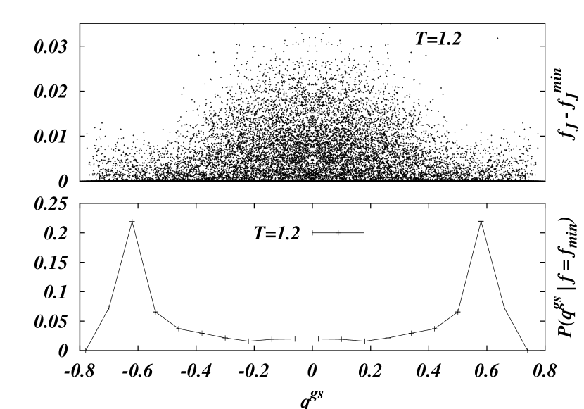
FIG. 6.: Scatter plot (upper panel) of the free energy density $f^{\alpha}_{J}-f^{min}_{J}$ of each equilibrium state at temperature $T=1.2$ vs. overlap with the sample ground state $q^{gs}_{J\alpha}(0,T)$. Here $N=150$ and the results of $1000$ different samples are superimposed. In the lower panel we display the averaged probability distribution function defined in (13) (see text).

FIG. 7.: Average ground state energy for sizes ranging from $N=19$ to $N=199$. We label with Cooling the output of our algorithm and with True the exact ground state. We have averaged each point over $1000$ samples. In inset we show the difference of the two results.

FIG. 8.: In the main body of this figure we display the averaged overlap $q^{gs}(0,T)$ vs. $T$. The upper curve is the same in Fig. 3 for $N=150$ (here we have reduced the number of considered temperatures), while the lower curve is obtained considering only the lowest free energy states. In inset we display the free energy difference $f_{min}-f_{heated}$ as a function of T.

$N$	$\Delta q^{gs}$	$\#\mathrm{jumps}$	$\#\mathrm{samples}$
50	0.149(4)	0.78(1)	10000
75	0.154(4)	0.82(1)	10000
100	0.150(4)	0.86(1)	10000
125	0.149(4)	0.90(1)	10000
150	0.147(4)	0.95(1)	10000
175	0.144(8)	0.97(1)	20000
200	0.14(1)	1.00(2)	17186

TABLE I.: In this table we display the results for the average size $\Delta q^{gs}$ of the jumps (second column), and the average number of jumps per sample (third column). The number of samples considered is in the fourth column.

REFERENCES

- [1] Email: mulet@ictp.trieste.it Permanent Address: Superconductivity Laboratory, Physics Faculty - IMRE, University of Havana, CP 10400, La Habana, Cuba.
- [2] Email: andrea.pagnani@roma1.infn.it
- [3] Email: giorgio.parisi@roma1.infn.it
- [4] K. Binder and A. P. Young, Rev. Mod. Phys. 58, 801 (1986); M. Mézard, G. Parisi and M. A. Virasoro, Spin Glass Theory and Beyond (World Scientific, Singapore 1987); K. H. Fisher and J. A. Hertz, Spin Glasses (Cambridge University Press, Cambridge U.K. 1991).
- [5] D.J. Thouless, P.W. Anderson, and R.G. Palmer, Phil. Mag. 35, 593 (1987).
- [6] A.J. Bray, and M.A. Moore, J. Phys. C: Solid State Phys. 12 L441 (1979); ibid. 13 L469 (1980).
- [7] K. Nemoto, and H. Takayama, J. Phys. C: Solid State Phys. 18 L529 (1985).
- [8] A.J. Bray, H. Sompolinsky, and C. Yu, J. Phys. C: Solid State Phys. 19 6389 (1986).
- [9] H. Takayama, and K. Nemoto, J. Phys.: Condens. Matter 2 1997 (1990).
- [10] M. Guagnelli, E. Marinari, and G. Parisi, J. Phys. A: Math. Gen. 26 5675 (1993); D. Lancaster, E. Marinari, and G. Parisi, ibid. 28, 3959 (1995).
- [11] D.S. Fisher and D.A. Huse, Phys. Rev. Lett. 56 1601 (1986).
- [12] A.J. Bray and M.A. Moore, Phys. Rev. Lett. 58, 57 (1987).
- [13] D.S. Fisher and D.A. Huse, Phys. Rev. B 38, 373 (1988).
- [14] K. Jonason, E. Vincent, J. Hammam, J.P. Bouchaud, and P. Nordblad, Phys. Rev. Lett. 81, 3243 (1998).
- [15] J.-P. Bouchaud in Soft and Fragile Matter, ed: M.E. Cates and M.R. Evans (Institute of Physic Publishing, Bristol and Philadelphia, 2000).
- [16] L.F. Cugliandolo and J. Kurchan, Phys. Rev. B 60, 922 (1999).
- [17] H. Rieger, L. Santen, U. Blasum, M. Diehl, and M. Jünger, J. Phys. A: Math. Gen. 29 3939 (1996).
- [18] I. Kondor, J. Phys. A: Math. Gen. 22, L163 (1989).
- [19] I. Kondor and A. Végsö, J. Phys. A: Math. Gen. 26, L641 (1993).
- [20] S. Franz and M. Ney-Nifle, J. Phys. A: Math. Gen. 28, 2499 (1995).
- [21] S. Franz, G. Parisi and M.A. Virasoro, J. Physique I 2, 1969 (1992).
- [22] T. Rizzo, Modelli di vetri di spin in campo medio: caos in temperatura, Tesi di Laurea, Università di Roma “La Sapienza” (1999).
- [23] F. Ritort, Phys. Rev. B 50, 6844 (1994).
- [24] M. Ney-Nifle, Phys. Rev. B 57, 492 (1998).
- [25] M. Ney-Nifle and A.P. Young, J. Phys. A: Math. Gen. 30, 5311 (1997).
- [26] J. Kisker, L. Santen, M. Schreckenberg, and H. Rieger Phys. Rev. B 53 6418 (1996).
- [27] A. Billoire and E. Marinari, J. Phys. A: Math. Gen. 33, L265 (2000).
- [28] K. Nishimura, K. Nemoto, and H. Takayama, J. Phys. A: Math. Gen. 23 5915 (1990).
- [29] M.L. Mehta, Random Martices and the Statistical Theory of Energy Levels, (Academic Press, New York, 1991).
- [30] C. De Dominicis and A.P. Young, J. Phys. A: Math. Gen. 16 2063 (1983).
- [31] H. Yoshizawa, and D.P. Belanger, Phys. Rev. B 30 5220 (1984); C. Ro, G.S. Grest, C.M. Soulolis, and K. Levin, Phys. Rev. B 31 1682 (1985).
- [32] W.H. Press, S.A. Teukolsky, W.T. Wetterling, and B.P. Flannery, Numerical Recipes in C. The Art of Scientific Computing, (Cambridge Univeristy Press, 1992).
- [33] The Reluctant algorithm works as follows: We generate random , then we calculate the local magnetic fields . We are interested in reducing to zero the number of spins opposite to the local fields, so that as a Reluctant strategy each time we flip the spin relative to the smaller (with regard to its absolute value) local field , then we calculate again the local fields until all spins are aligned with their local fields. We iterate this procedure until we find for times the same lower energy state. This procedure was introduced by G. Parisi in On the Statistical Properties of the Large Time Zero Temperature Dynamics of the SK Model, cond-mat/9501045.