Alternating-Spin Ladders in a Magnetic Field: New Magnetization Plateaux

Abstract

We study numerically the formation of magnetization plateaux with the Lanczos method in 2-leg ladders with mixed spins of magnitudes $(S_{1},S_{2})=(1,1/2)$ located at alternating positions along the ladder and with dimerization $\gamma$. For interchain coupling $J^{\prime}>0$ and $\gamma=0$, we find normalized plateaux at $m=1/3$ starting at zero field and $m=1$ (saturation), while when $\gamma\neq 0$ is columnar, another extra plateau at $m=2/3$ shows up. For $J^{\prime}<0$, when $\gamma<\gamma_{c}(J^{\prime})$ we find no plateau while for $\gamma>\gamma_{c}(J^{\prime})$ we find four plateaux at $m=0,1/3,2/3,1$. We also apply several approximate analytical methods (Spin Wave Theory, Low-Energy Effective Hamiltonians and Bosonization) to understand these findings and to conjeture the behaviour of ferrimagnetic ladders with a bigger number of legs.

]

I Introduction

Low dimensional spin systems has attracted many interests in recent years. It is the dominant effect of quantum fluctuation which distinguishes them from the classical picture which is valid for higher dimensions. For instance it was argued by Haldane[1] that integer spin chains have an energy gap between the ground state and the first excited state. In the presence of magnetic field, the energy gap persists up to a critical field, equal to the gap. For $S$=1 Anti-Ferromagnetic Heisenberg (AFH) chain the spectrum is gapless from the critical field up to the saturation field[2]. The $S$=1/2 AFH chain remains gapless from zero field up to the saturation field, where the ground state is fully polarized[3]. The situation might be more complex when one considers non-nearest neighbour interactions or non-homogeneous spin system by considering Bond-Alternations (BA) or different kind of spins. However a similar information may be obtained about the full spectrum by study the magnetization of system in the presence of a magnetic field.

The study of the magnetization process in one-dimensional quantum spin systems has been spured since the discovery of quantized plateaux in the magnetization curves as a function of the applied magnetic field [4],[5],[6]. This behaviour is a sort of “magnetic analogy” of the Quantum Hall Effect for charge degrees of freedom and it has become an issue of both theoretical and experimental interest. Likewise, 1d-chains with alternating mixed spins have been shown to behave with unusual quantum properties: they show ferrimagnetic behaviour instead of antiferromagnetism [7]-[11]. For instance for low spin values of ($S_{1},S_{2}$) ferrimagnetic chain ($S_{1}\neq S_{2}$) the low energy spectrum is gapless while there is a gap above this spectrum. Thus, a natural question arises as to whether ferrimagnetic systems are on equal footing with AF systems as far as the formation of magnetization plateaux is concerned. Here a remark is in order. As an alternating spin chain has an ordered ground state (GS) with total spin $S={N\over 2}(S_{1}-S_{2})$, then a natural plateau is expected even at zero field. Being this GS magnetization quite robust, a possible scenario for quantum ferrimagnets is that no other plateaux will appear, in addition to the saturation one. We shall show that this is not the case.

Although there are recent studies of one-chain ferrimagnets with magnetic fields [12],[13], to our knowledge little is known about the onset of magnetization plateaux in ferrimagnetic ladders. A ferrimagnetic ladder may be regarded as the first step to consider the interaction between ferrimagnetic chains as shown in Fig.1. This structure exists in $MnCu(pbaOH)(H_{2}O)_{3}$ where it is composed of parallel planes containing ferrimagnetic chains and in each plane the interaction between chains is assumed to be smaller than the intra-chain interactions[14]. In this paper we address the study of ferrimagnetic ladders under several situations of the Anti- ($J^{\prime}>0$) and Ferro-magnetic ($J^{\prime}<0$) interchain coupling and $\gamma$ dimerization patterns, which reveal a very reach structure of plateaux at fractional values of the full magnetization.

We define the total magnetization $M$ per unit length as follows,

$$M={1\over L}\sum_{\alpha=1}^{2}\sum_{n=1}^{L}\langle S_{1}^{(\alpha)z}(n)+S_{2}^{(\alpha)z}(n)\rangle\;,$$ (1)

where ${\bf S}^{(\alpha)}_{1}(n)$ denotes the quantum spin-$1$ at site $n$ in the leg $\alpha=1,2$ of the ladder, similarly ${\bf S}^{(\alpha)}_{2}(n)$ for the spin-$1/2$ and the number of sites is $N=2\times L$, $L$ is the number of rungs. Alternatively we may use $m$, the normalized value of the magnetization with respect to the saturation value as $m=M/M_{sat}$. We want to study this observable in a 2-leg ferrimagnetic ladder with the following Heisenberg Hamiltonian ($i=2n+\alpha$),

$$H = J\sum_{\alpha=1}^{2}\sum_{n=1}^{{L\over 2}-1}\;(\;[1+\gamma^{(\alpha)}(i)]\;\;{\bf S}^{(\alpha)}_{1}(i)\cdot{\bf S}^{(\alpha)}_{2}(i+1)$$ (2)

$$+ [1+\gamma^{(\alpha)}(i+1)]\;\;{\bf S}^{(\alpha)}_{2}(i+1)\cdot{\bf S}^{(\alpha)}_{1}(i+2)\;)$$ (3)

$$+ J^{\prime}\sum_{\alpha\neq\beta}^{1,2}\sum_{n=1}^{L}{\bf S}^{(\alpha)}_{1}(n)\cdot{\bf S}^{(\beta)}_{2}(n)-hS^{z}_{total}\;,$$ (4)

where $h$ is the magnetic field, $J$ and $J^{\prime}$ are coupling constants along the legs and the rungs respectively, and $\gamma^{(\alpha)}(n)$ is the dimerization patterns. We consider two different dimerization patterns : i) CBA (Columnar Bond Alternation, Fig.1-(a)) for which $\gamma^{(\alpha)}(n)=(-1)^{n+1}\gamma$ [15], and ii) SBA (Staggered Bond Alternation, Fig.1-(b)) where $\gamma^{(\alpha)}(n)=(-1)^{\alpha+1+n}\gamma$ [15]. We use periodic boundary conditions along the legs of the ladder.

The paper is organized as follows. In the next section we show the application of spin wave theory to derive the saturation field. In Sec. III we obtain a low-energy effective Hamiltonian based on Quantum Renormalization Group (QRG) formalism to describe the magnetization curve and give a conjecture for a $2n$-leg ferrimagnetic ladder. We present an Abelian Bosonization in Sec. IV to support our conjecture and express the necessary condition for the appearance of the magnetization plateaux in a $2n$-leg ferrimagnetic ladder. In Sec. V we will confirm the results of the analytical methods using a numerical method (Lanczos method) applied to a 2-leg ladder under a variety of situations. Finally, we summerize our results as a conclusion in Sec. VI.

II Spin Wave Theory

We start considering the case $J^{\prime}>0$. Then, since the GS is an ordered state with non-vanishing magnetization, it is natural to apply SWT to study the low energy properties of these ladders and predict correctly their ferrimagnetic behaviour. Now we extend this analysis including the effect of the external magnetic field. For weak magnetic fields we expect that the ferrimagnetic GS will be little perturbed so that it is still a good choice to make a SWT analysis around a partially polarized state with magnetization $S^{z}_{GS}={N\over 2}(S_{1}-S_{2})$. At $h=0$ the 2-leg ladder presents two pairs of branches, say $\omega_{A}^{(\pm)}(k;h=0),\omega_{B}^{(\pm)}(k;h=0)$, in the dispersion relation, namely:

$$\omega_{A}^{(\pm)}(k;0)=\frac{1}{2}(C_{1}-C_{2}+\sqrt{(C_{1}+C_{2})^{2}-4C_{3}^{2(\pm)}(k)}),$$ (5)

$$\omega_{B}^{(\pm)}(k;0)=\frac{1}{2}(C_{2}-C_{1}+\sqrt{(C_{1}+C_{2})^{2}-4C_{3}^{2(\pm)}(k)}),$$ (6)

$$C_{1}=(2J+J^{\prime})S_{1}\;\;\;;\;\;\;C_{2}=(2J+J^{\prime})S_{2}\;,$$ (7)

$$C_{3}^{(\pm)}(k)=\sqrt{S_{1}S_{2}}(2J\cos k\pm J^{\prime})\;.$$ (8)

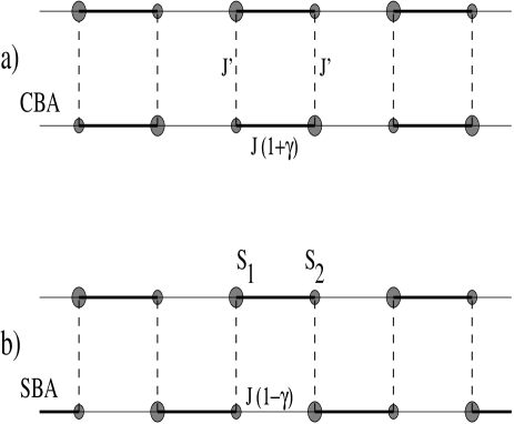
FIG. 1.: A picture of the dimerization patterns considered in a 2-leg mixed spin ladder: a) Columnar Bond Alternation (CBA), b) Staggered Bond Alternation (SBA).

For $J^{\prime}=0$ the two chains decouple and the branches collapse by pairs reproducing the one-chain result. When $h$ is applied the spectrum (6) is modified as follows:

$$\omega_{A}^{(\pm)}(k;h)=\omega_{A}^{(\pm)}(k;h=0)-h\;,$$ (9)

$$\omega_{B}^{(\pm)}(k;h)=\omega_{B}^{(\pm)}(k;h=0)+h\;,$$ (10)

After doing this analysis we find that the Bogoliubov transformation to diagonalize the SWT Hamiltonian is independent of $h$. This fact implies that we cannot see the plateaux of the curves $M=M(h)$ using this SWT.

For strong magnetic fields the previous ferrimagnetic GS is not a good choice to perturb around. It is more natural to choose a fully polarized (ferromagnetic) state with total magnetization $S^{z}_{GS}={N\over 2}(S_{1}+S_{2})$. We find that the SWT analysis yields the following spectrum:

$$\Omega_{A}^{(\pm)}(k;0) = \frac{1}{2}(-(C_{1}+C_{2})\pm\sqrt{(C_{1}+C_{2})^{2}-D^{(+)}(k)}),$$ (11)

$$\Omega_{B}^{(\pm)}(k;0) = \frac{1}{2}(-(C_{1}+C_{2})\pm\sqrt{(C_{1}+C_{2})^{2}-D^{(-)}(k)}),$$ (12)

$$D^{(\pm)}(k) = 16JS_{1}S_{2}(J\pm J\cos k+J^{\prime})(1\mp\cos k).$$ (13)

The inclusion of the magnetic field merely shifts this spectrum by $h$:

$$\Omega_{A}^{(\pm)}(k;h)=\Omega_{A}^{(\pm)}(k;h=0)+h\;,$$ (14)

$$\Omega_{B}^{(\pm)}(k;h)=\Omega_{B}^{(\pm)}(k;h=0)+h\;.$$ (15)

Again, we are not able to detect magnetization plateaux. However, now we can give a reliable prediction for the location of the saturation field $h_{sat}$. This happens when $\Omega_{A}^{(-)}(k=0;h_{sat})\equiv 0$, giving us the following relation for $S_{1}=1,S_{2}=1/2$ and normalizing $J=1$:

$$h^{sat}={3\over 2}(2+J^{\prime}).$$ (16)

We shall find that this condition is verified numerically. For decoupled chains $J^{\prime}=0$ we reproduce the one-chain results [13]. Similarly, for ferromagnetic coupling $J^{\prime}<0$ we find the following saturation field,

$$h_{sat}={3\over 4}\left((2+J^{\prime})+\sqrt{(2+J^{\prime})^{2}-{64J^{\prime}\over 9}}\right).$$ (17)

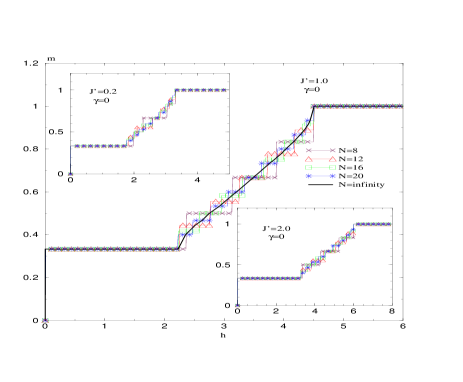
FIG. 2.: Magnetization plateaux for alternating 2-leg ladder: $\gamma=0$, $J^{\prime}=0.2,1.0,2.0$. There are two plateaux at $m=1/3\;,\;1$.

III Low Energy Effective Hamiltonian

In order to explain qualitatively the onset of magnetization plateaux in a 2-leg ferrimagnetic ladder we can use an RG transformation to map the original model (4) onto a one-chain model with known properties. To perform the block RG transformation we choose as the building block the unit cell made up of 2 spins $(S_{1}=1,S_{2}=1/2)$. The block Hamiltonian is then $h^{B}=J^{\prime}{\bf S}_{1}\cdot{\bf S}_{2}-h(S_{1}^{z}+S_{2}^{2})$. For simplicity, we assume a strong coupling regime $J^{\prime}\gg J$. This allows us to place $h^{B}$ on the vertical rungs of the 2-leg ladder so that the whole block Hamiltonian is the rung Hamiltonian ($H^{B}=H_{r}$) and the inter-block Hamiltonian is the leg Hamiltonian ($H^{BB}=H_{l}$). We need to distinguish 2 regimes of magnetic field to construct the truncation operator. a) For low fields, namely $h<3/2J^{\prime}$, the lowest lying states of $h^{B}$ is a spin-1/2 doublet. Then we use this to map (4) onto the following low-energy effective Hamiltonian ($J=1$):

$$H_{eff}=-LJ^{\prime}- {4\over 9} \sum_{n=1}^{L}\gamma^{\prime}_{n}\ {\bf S}^{\prime}_{n}\cdot{\bf S}^{\prime}_{n+1}-h\sum_{n=1}^{L}S^{\prime z}_{n}\;,$$ (18)

$$\gamma^{\prime}_{n} = \sum_{\alpha=1}^{2}(1+\gamma^{(\alpha)}(n))\;,$$ (19)

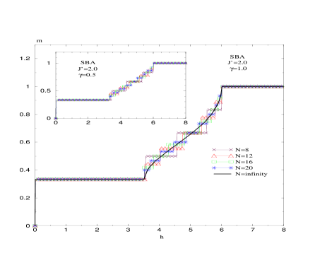
FIG. 3.: Magnetization curves for SBA configuration with $J^{\prime}=2.0$, $\gamma=1.0,0.5$ which shows only two plateaux at $m=1/3\;,\;1$.

$H_{eff}$ is a spin (${\bf S}^{\prime}=$) 1/2 Ferromagnetic Heisenberg chain in the presence of an external magnetic field, which shows a ferromagnetic phase with $M=1/2\ (m=1/3)$.

b) For high fields, namely $h>3/2J$, the lowest two energy states of $h^{B}$ have now spin quantum numbers $|S_{T}=1/2,S^{z}_{T}=+1/2\rangle$, $|3/2,+3/2\rangle$. Upon projection of (4) onto this subspace we arrive at the following effective Hamiltonian ($J=1$):

$$H_{eff}=-({J^{\prime}\over 4}+h)L+{5\over 36}\sum_{n=1}^{L}\gamma^{\prime}_{n}+H_{XXZ+h}\;,$$ (20)

where $H_{XXZ+h}$ is an AF spin 1/2 Heisenberg model in a magnetic field with coupling parameters given by:

$$H_{XXZ+h} = {2\over 3}\sum_{n=1}^{L}\gamma^{\prime}_{n}(\sum_{\mu=x,y}S_{n}^{\prime\mu}S^{\prime\mu}_{n+1}+\Delta S_{n}^{\prime z}S^{\prime z}_{n+1})-h^{\prime}_{n}S^{\prime z}_{n}\;,$$ (21)

$$\Delta = {1\over 3}\;\;\;\;;\;\;\;\;h^{\prime}_{n}={3\over 2}h-{11\over 6}\gamma^{\prime}_{n}-{9\over 4}J^{\prime}\;,$$ (22)

In the absence of dimerization $\gamma=0$ or when the dimerization pattern is SBA, we have $\gamma^{\prime}_{n}=2$ constant and thus the effective field $h^{\prime}$ is also uniform. In this case we can use the knowledge of the $H_{XXZ+h}$ model to predict the existence of 2 plateaux. It is known that this model has a critical value for $h^{\prime}$ where a phase transition occurs between the Partially Magnetized (PM) to the Saturated Ferromagnetic (SF) states. This critical line in the $\Delta-h^{\prime}$ phase diagram is given by [16] $h^{\prime}_{c}=\Delta+1$ (for $h^{\prime}>0$). Firstly, we find that the relation between the magnetization $M$ of the original ferrimagnetic ladder and the magnetization $M_{XXZ}$ of the effective XXZ model is:

$$M=1+M_{XXZ}.$$ (23)

Now it is possible to derive the dependence of $M$ on $h$. By using the relation in (22) we find two critical fields given by $h_{c1}={2\over 3}+{3\over 2}J^{\prime}$ and $h_{c2}={38\over 9}+{3\over 2}J^{\prime}$ such that for $h\leq h_{c1}$ then $M=1/2$, for $h_{c1}\leq h\leq h_{c2}$ then $1/2\leq M\leq 3/2$ and for $h\geq h_{c2}$ then $M=3/2$. Therefore, we find a good qualitative picture of the $M(h)$-plot with two plateaux at normalized values of $m=1/3$ and $m=1$ [17]. This agrees with the numerical results in Fig. 1 and Fig. 2 using Lanczos.

Although the knowledge of known models obtained in Eqs.(19,22) was used to explain the magnetization curve one may however continue using QRG for Eqs.(19,22) to obtain the RG-flow of coupling constants and finally the magnetization curve. In the case of Eq.(19) the Hamiltonian will be projected to another ferromagnetic Heisenberg model with larger spins. By repeating this procedure one will arrive at the classical ferromagnetic Heisenberg fixed point. In the other case in Eq.(22), the RG-flow will describe both the partially magnetized and the fully polarized state of the $XXZ+h$ model [18]. Needless to say that the final result will not change.

Furthermore, if we restrict ourselves to a strong coupling analysis, we can extend this QRG analysis in a simple way to ferrimagnetic ladders with a number of legs given by $n_{l}\equiv 2n$ in order to preserve the structure of $(S_{1},S_{2})$-cells in both directions. Then, in each rung the highest total spin is $n(S_{1}+S_{2})$ and when we apply a $h$ field we find that the allowed values of $M$ are $-n(S_{1}+S_{2}),-n(S_{1}+S_{2})+1,\ldots,n(S_{1}+S_{2})-1,n(S_{1}+S_{2})$. Upon normalization to the highest value, we get that the allowed values of $m$ are:

$$-1,-1+{1\over n(S_{1}+S_{2})},\ldots,+1-{1\over n(S_{1}+S_{2})},+1\;.$$ (24)

Now, if we particularize to the case $S_{1}=1,S_{2}=1/2$, we find $-1,-1+2/3n,\ldots,+1-2/3n,+1$. We can readily check that in this set the values 1/3 and 1 are always present. Moreover, we may conjeture the existence of additional plateaux if the number of legs increases.

IV Abelian Bosonization

We may re-obtain this quantization condition using a heuristic argument based on Abelian Bosonization, as in the original OYA argument [5]. This has been carried out with full detail for standard AF spin-1/2 ladders in refs. [19]. For simplicity, let us consider first a one-chain ferrimagnet ($J^{\prime}>0$) with spins $(S_{1},S_{2})$ in the unit cell and no dimerization $\gamma=0$. This unit cell will play the role of an effective site in the bosonization. Firstly, the spin chain is fermionized by introducing colored fermions $\psi_{n}^{(i),c_{i}}$, $i=1,2$, with color index $c_{i}=1,\ldots,2S_{i}$ to describe the spin degrees of freedom of $S_{1}$ and $S_{2}$, respectively. We make the usual assumption about the continuum limit: only excitations close to the Fermi points are important. Thus, we introduce slowly varying Left and Right fermionic fields $\psi_{L,R}^{(i),c_{i}}(x)$, $i=1,2$ such that $\psi_{n}^{(i),c_{i}}\sim e^{ik_{F}x}\psi_{R}^{(i),c_{i}}(x)+e^{-ik_{F}x}\psi_{L}^{(i),c_{i}}(x)$. Then, the bosonization proceeds in a standard fashion representing these fermions by vertex operators in terms of chiral boson fields $\phi_{L,R}^{(i),c_{i}}$ as $\psi_{L,R}^{(i),c_{i}}(x)=e^{\mp i\phi_{L,R}^{(i),c_{i}}/R}$, respectively, and $R$ is the compactification radius of the boson. In this low energy analysis, all potentially massive modes will decouple and only the massless bosons will contribute to this effective description. This is the case of the total diagonal boson $\Phi=\sum_{i=1,2}\sum_{c_{i}=1}^{2S_{i}}(\phi_{L}^{(i),c_{i}}+\phi_{R}^{(i),c_{i}})$. In terms of this boson, the translational symmetry by one unit cell of the original lattice chain is realized as a total shift $\Phi\rightarrow\Phi+2(S_{1}+S_{2})k_{F}2\pi R$. On the other hand, the Fermi momentum is modified by a shift of the magnetization as $k_{F}={\pi\over 2}(1-m)$ (the magnetic field acts as a chemical potential.) With these two conditions, a leading operator of the form $\cos(\Phi/R)$ will be compatible only if $(S_{1}+S_{2})(1-m)=\mbox{integer}$. This is the application of the OYA condition to ferrimagnetic systems.

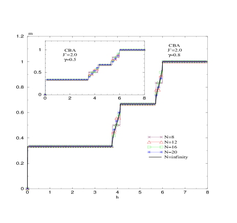
FIG. 4.: Magnetization plateaux for CBA configuration with $J^{\prime}=2.0$, $\gamma=0.8,0.5$. A new plateau appears at $m=2/3$, its width increases by increasing $\gamma$.

In our case, we have $S_{1}=1,S_{2}=1/2$ and this yields only $m=1/3,1$. This agrees with the QRG analysis [17] and with numerics [13]. We may attempt to go beyond this one-chain case to a set of $n$ 2-leg alternating ladders coupled together. In each 2-leg ladder we assume a strong coupling limit ($J^{\prime}\gg 1$) and place the unit cell $(S_{1},S_{2})$ on the rungs as in the RG analysis. Then, we assume a weak coupling ($J^{\prime}\ll 1$) among these set of $n$ ladders. Repeating the argument yields the following quantization condition for magnetization plateaux:

$$T_{u}(S_{1}+S_{2})\ n\ (1-m)=\mbox{integer}\;,$$ (25)

where we have introduced a “translational unit” $T_{u}$ to account for the translational symmetry of the ground state. In the original Hamiltonian we have $T_{u}=2$ but due to non-perturbative effects it can be different in the real ground state [6]. This condition (25) (with $T_{u}=1$) is precisely equivalent to eq. (22) [19]. We remark that this condition (25) appears as a necessary condition, but it is not sufficient. Additionally, the compactification radius should be greater than its critical value. Thus, we consider this quantization condition as a conjeture and we have applied the Lanczos method to test it.

V Numerical Results: The Lanczos Method

Now we present our numerical studies of 2-leg ladders with a number of sites $N=2\times L$ where $L=4,6,8,10$ (due to the constraint of periodic BC’s). We apply Lanczos to each $S^{z}$-sector of the Hilbert space from $S^{z}=0$ to $S^{z}={N\over 2}(S_{1}+S_{2})$. We always set $J=1$ and make $J^{\prime}$ range both in AF and Ferromagnetic regimes. The dimerization parameter $\gamma$ is also varied for both CBA and SBA patterns.

Firstly, we consider AF couplings ($J^{\prime}>0$) and vanishing dimerization ($\gamma=0$). In Fig.2 we show 3 plots of the magnetization curve for weak $J^{\prime}=0.2$, intermediate $J^{\prime}=1.0$ and strong coupling $J^{\prime}=2.0$. For weak coupling we find two plateaux at $m=1/3,1$ and values of $h_{c1},h_{c2}=h_{sat}$ very close to the pure 1d ferrimagnet. This amounts to a smooth evolution from the one-chain case. Moreover, at strong and intermediate couplings, the same picture holds true which supports our effective Hamiltonians (19),(20) based on the low-energy analysis. We have also checked numerically that the value of the saturation field $h_{sat}$ fits nicely the SWT result in eq. (16), as clearly shown in Fig.2. Another remarkable aspect of our plots is that they show a square-root behaviour of the magnetization $m-m_{c}\sim\sqrt{h^{2}-h^{2}_{c}}$ in the transient region near the critical points, as is also the case for standard AF spin-1/2 ladders [19]. Next, as a check of our numerical method, we consider SBA dimerization with $\gamma=1$ and $J^{\prime}=2.0$. In this situation the 2-leg ladder degenerates onto a one-chain ferrimagnet with coupling $J=2.0$ and in Fig.3 we reproduce exactly the existence of two plateaux and the value of the saturation field $h_{sat}=3$ (in units $J=2$.) We find that this SBA picture is robust by plotting the case $\gamma=0.5$.

In order to see the effect of different dimerization patterns in the formation of the magnetization plateaux, we have also studied the CBA dimerization configuration. We plot the case CBA for $J^{\prime}=2.0$ and $\gamma=0.5,0.8$ in Fig.4. Interestingly enough, we clearly find a new plateau at $m=2/3$ in addition to the previous ones at $m=1/3$ and $m=1$. This agrees with eq. (25) with $T_{u}=2$. The width of this new plateau grows with increasing dimerization. The new plateau shows the appearance of an energy gap between the two energy bands in the spectrum of CBA configuration. This picture is true for CBA configuration ($J^{\prime}>0$) when $\gamma\neq 1$. By setting $\gamma=1$ the ladder will be decomposed to isolated 4-sites plaquette which does not reflect the properties of a system in the thermodynamic limit ($N\rightarrow\infty$).

Secondly, we consider Ferromagnetic couplings ($J^{\prime}<0$) with different dimerizations. In this case the CBA pattern is more interesting for we have found that it exhibits two phases, one gapless for $\gamma<\gamma_{c}$ and another gapped for $\gamma>\gamma_{c}$, in the $J^{\prime}-\gamma$ diagram with a phase-separating line which goes as $\gamma_{c}\sim 0.42$ when $J^{\prime}\rightarrow-\infty$ [15].

In Fig.5 we consider a plot for $J^{\prime}=-1.0$ and $\gamma=0.2$ which happens to be in the gapless phase. Accordingly with this behaviour, there is no plateau at $m=0$ and the transient region immediately starts at $h=0$. Moreover, the previously robust $1/3$-magnetization plateau is now absent. The reason for this is because now the GS has no longer total spin ${N\over 2}(S_{1}-S2)$ but $0$. This is completely in agreement with the effective Hamiltonian which has been obtained for this region in [15]. The effective Hamiltonian for CBA configuration ($J^{\prime}<0$) and $\gamma<\gamma_{c}$ is a bond-alternation spin 3/2 AFH model in the gapless phase [15]. It has been shown that the gapless phase of spin 3/2 AFH chain is in the universality class of a spin 1/2 AFH chain[20]. As it has been noted in the introduction the model has no plateau in the magnetization curve up to the saturation field.

Finally, we consider the opposite case of parameters corresponding to the gapped phase, namely $J^{\prime}=-1.0$ and $\gamma=0.8$, in Fig.6.

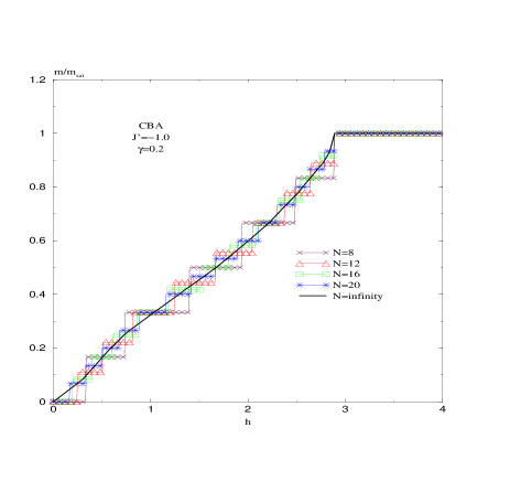
FIG. 5.: Magnetization curves for ferro CBA ladders with $J^{\prime}=-1.0$, $\gamma=0.2$. There is no plateau which reveals no gap in the full spectrum.

This plot shows a very rich structure. It shows four magnetization plateaux at $m=0,1/3,2/3,1$. Since the model has an energy gap in this region the $m=0$ plateau extends until the magnetic field closes the gap in the spectrum $h_{c}=\Delta$. More interesting is now the $m=1/3$ plateau, which is not natural for now the GS is not ferrimagnetic when $J^{\prime}<0$. In fact, this plateau does not start at $h=0$ as in Figs.2-4. To explain the nature of these plateaux we can resort to a strong coupling RG analysis and map the original Hamiltonian (4) onto a AFH one-chain of spins $3/2$ with dimerization (see eq.(5) in [15]) and apply the OYA argument. We have also checked that the saturation field $h_{sat}$ is also correctly predicted by SWT in eq. (17).

The situation of SBA at $J^{\prime}<0$ is similar to Fig.5. This can be understood by the effective low-energy Hamiltonian which is a homogenous spin 3/2 AFH chain[15]. The model is gapless for the whole range of magnetic field which results to no plateaux.

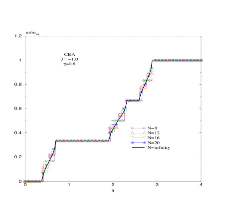
FIG. 6.: Magnetization plateaux for ferro CBA configurations with $J^{\prime}=-1.0$, $\gamma=0.8$. Four plateaux appear in this region at $m=0\;,1/3\;,2/3\;,1$.

VI Conclusions

We have addressed the study of alternating $(S_{1},S_{2})$-spin ladders in the presence of an external uniform magnetic field in a fixed direction. The low energy properties of this problem is relevant in understanding the behaviour of ferrimagnetic systems in magnetic fields as compared with the properties exhibited by more standard antiferromagnetic ladders.

In summary, we have shown that mixed-spin systems show extra magnetization plateaux in addition to the natural ones at $m=1/3\ \mbox{and}\ 1$ and we have presented a complete account for the diversity of plateaux-patterns when we vary the interchain and dimerization couplings.

We have undertaken a complete numerical study using the Lanczos method of the 2-leg ladders with alternating spins $S_{1}=1/2,S_{2}=1$, for several regimes of the interchain coupling constant $J^{\prime}$, both antiferro- and ferromagnetic, and for several types of dimerization patterns (CBA and SBA). In the antiferromagnetic regime ($J^{\prime}>0$) the SBA configuration shows only the natural plateaux at $m=1/3\ \mbox{and}\ 1$ while the CBA configuration shows an extra plateau at $m=2/3$. In the ferromagnetic regime ($J^{\prime}<0$) the SBA configuration shows no plateau where the model remains gapless from the zero field up to the saturation field. The CBA configuration in the $J^{\prime}<0$ regime has more interesting features. For $\gamma<\gamma_{c}$ the model is gapless for all range of magnetic field and results to no plateau, while for $\gamma>\gamma_{c}$ the model is gapful. Then the first plateau appears at $m=0$. There are also two other plateaux at $m=1/3\ \mbox{and}\ 2/3$ which are expressed by the dimerized $S$=3/2 AFH effective model. The trivial plateau at $m=1$ counts the number of plateaux to 4 in this case.

The magnetization curves obtained in this way provide a whole picture of the response of mixed-spin systems to external magnetic fields.

We have complemented these numerical studies with additional analytical methods such as Spin Wave Theory (in two fashions), effective low-energy mappings of the type used in Quantum RG methods and Abelian Bosonization. Although none of these analytical methods provide a complete understanding of the problem, they however give us some useful partial knowledge that fits nicely into our findings obtained with numerical methods.

Concerning the possible experimental realization of the magnetic ferriladders studied in this work, we would like to point out that the field of organic chemistry is a likely candidate for synthesizing this type of materials [21, 22, 23].

Acknowledgements We acknowledge discussions with M. Abolfath, H. Hamidian and G. Sierra, and the Centro de Supercomputación Complutense for the allocation of CPU time in the SG-Origin 2000 Parallel Computer and Max-Planck-Institut für Physik komplexer Systeme for computer time. M.A.M.-D. was supported by the DGES spanish grant PB97-1190.

REFERENCES

- [1] F. D. M. Haldane, Phys. Lett. A93, 464 (1983).
- [2] T. Sakai and M. Takahashi, Phys. Rev. B43, 13383 (1991).
- [3] R. B. Griffiths, Phys. Rev. 133, A768 (1964).
- [4] K. Hida, J. Phys. Soc. Jpn. 63, 2359 (1994).
- [5] M. Oshikawa, M. Yamanaka and I. Affleck, Phys. Rev. Lett. 78, 1984 (1997).
- [6] K. Totsuka, Phys. Lett. A228, 103 (1997); Phys. Rev. B57, 3454 (1998)
- [7] M. Drillon, J. C. Gianduzzo and R. Georges, Phys. Lett. A96, 413 (1983). V. N. Krivoruchko, Fiz. Nizk. Temp. 14, 844 (1989);
- [8] S. K. Pati, S. Ramasesha, and D. Sen, Phys. Rev. B 55, 8894 (1997). J. Phys. Cond. Matt. 9, 8707 (1997);
- [9] S. Yamamoto, S. Brehmer and H.-J. Mikeska Phys. Rev. B57, 13610 (1998); S. Yamamoto and T. Fukui, Phys. Rev. B57, R14008 (1998); S. Yamamoto, T. Fukui, K. Maisinger and U. Schollwock, J. Phys. Cond. Matt. 10, 11033 (1998).
- [10] A. K. Kolezhuk, H.-J. Mikeska, and S. Yamamoto, Phys. Rev. B55, R3336 (1997).
- [11] S. Brehmer, H.-J. Mikeska and S. Yamamoto, J. Phys. Cond. Matt. 9, 3921 (1997);
- [12] K. Maisinger et al., cond-mat/9805376.
- [13] T. Sakai and S. Yamamoto, Phys. Rev. B60, 4053 (1999).
- [14] O. Kahn, Y. Pei, M. Verdaguer, J.P. Renard and J. Sletten, J. Am. Chem. Soc. 110, 782 (1988).
- [15] A. Langari, M. Abolfath and M.A. Martin-Delgado, Phys. Rev. B61, 343 (2000).
- [16] C.N. Yang and C. P. Yang, Phys. Rev. 150, 321 (1966).
- [17] We have performed the same QRG analysis for a one-chain finding the same picture of two plateaux at but with different values of . This agrees with numerical results.
- [18] A. Langari, Phys. Rev. B58, 14467 (1998).
- [19] D. C. Cabra, A. Honecker and P. Pujol, Phys. Rev. Lett. 79, 5126 (1997); Phys. Rev. B58, 6241 (1998).
- [20] S. Yamamoto, Phys. Rev. B55, 3603 (1997).
- [21] A. Canishi et al. Inorg. Chem. 27, 1756 (1988).
- [22] Y. Hosokoshi et al., Phys. Rev. B60, 12924 (1999).
- [23] M. Nishizawa et al., J. Phys. Chem. B104, 503 (2000).