Polymer Films in the Normal-Liquid and Supercooled State:
A Review of Recent Monte Carlo Simulation Results

Abstract

The present paper reviews recent attempts to study the development of glassy behavior in thin polymer films by means of Monte Carlo simulations. The simulations employ a version of the bond-fluctuation lattice model, in which the glass transition is driven by the competition between an increase of the local volume requirement of a bond, caused by a stiffening of the polymer backbone, and the dense packing of the chains in the melt. The melt is geometrically confined between two impenetrable walls separated by distances that range from once to about fifteen times the bulk radius of gyration. The confinement influences static and dynamic properties of the films: Chains close to the walls preferentially orient parallel to it. This orientation tendency propagates through the film and leads to a layer structure at low temperatures and small thicknesses. The layer structure strongly suppresses out-of-plane reorientations of the chains. In-plane reorientations have to take place in a high density environment which gives rise to an increase of the corresponding relaxation times. On the other hand, local density fluctuations are enhanced if the film thickness and the temperature decrease. This implies a reduction of the glass transition temperature with decreasing film thickness.

I Introduction and Overview

Many recent studies deal with the influence of confinement on the dynamic behavior of glass forming liquids [1, 2]. Besides the practical importance of such systems (polymer films as protective coatings, flow through porous materials, etc.) one motivation for this research is that it might also provide a better understanding of the glass transition in the bulk [1, 3, 4, 5]. If the glass transition was driven by an underlying correlation length $\xi$ which grows with progressive supercooling towards the transition temperature $T_{\rm g}$, confinement should truncate the growth as soon as $\xi$ becomes comparable to the size, $L$, of the restrictive geometry. Marked deviations from the bulk behavior are then expected.

However, the trend of these deviations is not obvious. Should the dynamics be accelerated or slowed down? Theoretical arguments may be put forward for both scenarios. For instance, one could speculate that the glass transition is caused by some subtle kind of static order which characterizes the spatial arrangement of the particles in the glassy phase and spontaneously develops during supercooling. The correlation length should then measure the growth of these (solid-like) regions. If this was true, one could invoke an analogy to the theory of spin glasses [6] and suggest that the structural relaxation time $\tau$ scales as $\tau\sim\xi^{z}$ ($z$ being a dynamic critical exponent). When $\xi\simeq L$, $\tau$ should level off and the dynamics should become faster in confined geometry. On the other hand, one can also adopt the point of view that supercooling makes the dynamics of a glass former become progressively cooperative. Cooperativity means that the displacement of a particle is predicated upon the simultaneous rearrangement of many neighboring particles and the correlation length measures the spatial extent for these cooperative processes. There is evidence for such a dynamic heterogeneity from recent simulations [7, 8, 9, 10, 11, 12] and experiments [13, 14, 15, 16]. In spatial confinement some of these processes should be suppressed. Therefore, one expects $\tau$ to increase and the dynamics to slow down compared to the unrestricted bulk.

A variety of experiments [2, 17, 18, 19, 20, 21, 22, 23, 24, 25, 26, 27, 28], computer simulations [2, 29, 30, 31, 32, 33, 34, 35, 36, 37] and theoretical approaches [2, 38, 39, 40] have attempted to display the phenomenology and to elucidate the underlying mechanisms of dynamics in confinement. The systems studied range from simple liquids [29, 31, 32, 33, 34, 40], over molecular and hydrogen-bonded liquids [17, 18, 19, 20, 21, 35] to polymers [22, 23, 24, 25, 26, 27, 28, 36, 37, 39]. The geometries considered involve three-dimensional cavities [21, 31, 38], pores [17, 18, 19, 20, 34, 35], nano-sized fillers embedded in polymer melts [37], and thin films [22, 23, 24, 25, 26, 27, 28, 29, 30, 32, 33, 36, 39, 40], exhibiting different interactions between the glass former and the walls of the confinement. These interactions and the arrangement of the molecules close to the walls introduce boundary effects which perturb the bulk structure. These effects can reinforce or mask the influence of pure confinement on the dynamics. Therefore, a good knowledge and control of the surface properties is important for the interpretation of the results.

Such knowledge and control is typically available in computer simulations. Simulations study precisely defined – though often highly idealized – systems to reveal possible consequences of various kinds of confinement. A special kind of confinement which may only be realized in computer simulations is a size variation of the simulation box while maintaining periodic boundary conditions. This means the following: Usually, the simulated system is contained in a cubic box which is replicated in all spatial dimensions. If a particle leaves the box on one side, an identical image particle simultaneously enters the box from the opposite side. The simulation cell can thus be thought of as a section of a macroscopic system. The fact that the adjacent boxes are identical copies does not influence the physical properties of the system if the box size is large (and if there are no such complications, such as long-range interactions, spontaneous ordering close to phase transitions, etc.). However, if it shrinks, finite-size effects may occur. The development of such finite-size effects during supercooling has been observed in simulations of binary Lennard-Jones mixtures [41], of hard sphere mixtures [42, 43] and of silica [44, 45], and was also treated analytically [38]. Generally, one finds the dynamics to be slowed down with shrinking box size (see [41] for a comparative discussion of the results from Refs. [41] and [42]).

An important property of these studies is that the confinement is weak. There is no specific interaction with the boundary and no spatial arrangement close to the surface of the simulation box. Changes of the bulk structure are very mild or not present at all. The same situation is also realized in recent simulations of the relaxation dynamics in spherical cavities [31] and pores [34, 46]. In these studies, a sphere or a cylinder is cut out of a large bulk sample. Subsequently, only the inner particles are allowed to move, whereas the outer particles are frozen. They realize the walls of the confinement. Since the walls are rough and adapted to the liquid structure, a fluid particle can be trapped in cavities, into which it perfectly fits. Relaxation out of these traps is thus sluggish so that one finds a slowing down of the dynamics close to the walls. This slow relaxation also retards the dynamics of particles in the inner part of the liquid [34, 46].

While the impact of confinement on the structure is negligible in these studies, wall-induced perturbations of the bulk structure occur in simulations of thin film geometries. If the film geometry is realized by two free surfaces (freely standing films), the density of the liquid decreases from the bulk value to zero across the liquid/vacuum interface [29, 30, 47]. The interface sharpens with decreasing temperature. On the other hand, if the glass former is embedded between two impenetrable and smooth walls, there are pronounced density oscillations starting with a value larger than the bulk density at the wall. These oscillations can decay towards the bulk density with increasing distance from the wall or propagate through the film, depending on the film thickness and temperature considered. These structural differences also affect the dynamic behavior. For the freely standing films one generally finds that the particles closer to the interface are more mobile than inner particles which behaves bulk-like [29, 30, 47]. Therefore, the overall dynamics of the film is faster than the bulk at the same temperature. This should lead to a decrease of the average glass transition temperature. The same interpretation is also suggested by an analysis of recent experimental results for freely standing polystyrene films [26] and by comparitive computer simulations of freely standing and supported polymer film models [48].

Whereas the observed speeding up of the particle motion close to a free interface is intuitively expected, the situation is not so clear for glass formers confined between two completely smooth, impenetrable walls which exert no preferential attraction on the particles, but merely represent a geometric confinement. Simulations of glassy polymer films [49, 50] suggests an acceleration of the local relaxation dynamics, whereas simulations of binary hard sphere mixtures rather find a slowing down [32, 33]. A tentative explanation of this difference could be as follows: The aforementioned density oscillations are much more pronounced for the binary mixtures than for the polymer films. This is a consequence of the model parameters used in the simulations. For the mixtures there seem to be densely filled layers of particles stacked on top of each other at low temperature. Motion has to occur in this very high density environment which might therefore be slower than in the bulk and in the simulations of the polymer films.

Thin film geometries are also extensively studied experimentally, especially for polystyrene melts [22, 23, 24, 25, 26, 27, 28]. The geometries investigated range from freely standing films [23, 24, 25, 26] to supported films (two inequivalent surfaces: ${\rm SiO_{2}}$ and air) [22, 24, 25, 28] and polystyrene embedded between two ${\rm SiO_{2}}$ substrates, realized either by capping the film with another silicon-oxide layer [24] or by intercalating the polymer in layered-silicate hosts [27]. A systematic variation of film thickness and chain length has revealed many interesting results which have been summarized in recent comprehensive reviews [51, 52] and elicited theoretical explanations [39].

The present paper also deals with the glass transition of a thin polymer film. It presents Monte Carlo simulation results for a simple model of a non-entangled polymer melt confined between two solid walls. Its main focus is to investigate static and dynamic properties when polymer films of different thicknesses are progressively supercooled. The paper is organized as follows: Section II describes the background of the model and the employed simulation technique. Sections III and IV illustrate the influence of spatial confinement on the structure of the melt and the resulting consequences for the dynamic behavior. The last section V summarizes and discusses the results.

II Coarse-Grained Lattice Simulations of Polymer Films

The present approach uses a lattice model: the bond-fluctuation model [53, 54, 55]. This model is intermediate between a highly flexible continuum treatment and standard lattice models of polymers [56, 57, 58]. With the latter it has in common the simple lattice structure which is very efficient from a computational point of view [59]. However, it differs from them in that the set of bond vectors is not limited by the coordination number of the lattice, but much larger. In this respect, it resembles more a continuum model.

A monomer of the bond-fluctuation model does not directly correspond to a chemical monomer. It should rather be thought of as representing a group of chemical monomers (comprising typically $3$ to $5$ monomers for simple polymers, such as polyethylene [57, 60]). A lattice bond should thus be interpreted as the vector joining these groups. This coarse-grained vector can fluctuate in length and direction to a much larger extent than its chemical counterpart. The bond-fluctuation model accounts for this flexibility of the coarse-grained bond vector by associating a monomer not with a single lattice site, but with a unit cell of a simple cubic lattice. The monomers can be connected by 108 different bond vectors which are chosen such that local self-avoidance of the monomers and uncrossability of the bond vectors during the simulation are guaranteed.

Energy Function and Geometric Frustration. In addition to excluded volume interaction and chain connectivity an energy function ${\cal H}(\mbox{\boldmath$b$\unboldmath})$ is introduced for the bond vectors $b$. It favors bonds of length $b=3$ and directions along the lattice axes (${\cal H}(\mbox{\boldmath$b$\unboldmath})=0$) in comparison to the rest of available bond vectors (${\cal H}(\mbox{\boldmath$b$\unboldmath})=\epsilon$) [61, 62, 63]. Figure 1 illustrates the effect of this two-level Hamiltonian. If temperature decreases, each bond attempts to adopt the ground state ${\cal H}(\mbox{\boldmath$b$\unboldmath})=0$. A bond in the ground state blocks four lattice sites which can no longer be occupied by any other monomers due to the excluded volume interaction. This reduces the amount of accessible volume and generates a competition between the internal energy of a bond and the local arrangement of other monomers around it. This competition forces some bonds to remain in the excited state. They are geometrically frustrated [62, 63]. For instance, the bond of the lower chain in Fig. 1 could only reach the ground state if the monomer of the upper chain moved away. However, this motion is only possible if the constraints acting on this monomer are released which might in turn require the motion of further distant monomers. The relaxation of local geometric frustration is thus predicated upon the cooperative rearrangement of many monomers, which can become very sluggish due to mutual blocking at low temperatures. Therefore, the development of the geometric frustration during the cooling process causes the glassy behavior of the model. It is also the driving force which the Gibbs-Di Marzio theory makes responsible for the glass transition of polymer melts [64, 65, 66].

Monte Carlo Methods: Real versus Artificial Dynamics. The competition between energetic and packing constraints leads to a slow, glass-like structural relaxation of the melt if the usual bond-fluctuation dynamics is used. This dynamics consists of the following steps: First, a monomer and a lattice direction are chosen at random. Then, it is checked whether the targeted lattice sites are empty (excluded volume interaction) and whether the new bonds belong to the allowed set (maintenance of chain connectivity). If these conditions are satisfied, the energy change $\Delta E$ associated with a monomer displacement in the chosen lattice direction is calculated. The attempted move is accepted with probability $\min\left(1,\exp\left[-\beta\Delta E\right]\right)$ (Metropolis criterion [58, 67]), where $\beta=1/k_{\rm B}T$ is the reciprocal temperature (the temperature is measured in units of $\epsilon/k_{\rm B}$). These local moves are supposed to mimic a random force exerted on a monomer by its environment. They lead to Rouse-like dynamics which is typical of short polymers in dense melts [68, 69, 70].

The local dynamics gives rise to a strongly protracted structural relaxation of the melt. Although this is exactly the physical phenomenon that we are interested in, such a slow relaxation is very disadvantageous to quickly equilibrate the system during the cooling process. To circumvent this problem one can exploit the property of the Monte Carlo technique that the elementary move may be adapted at will. Since the final equilibrium state is independent of the way by which it was reached, the realistic local dynamics may be replaced by an artificial one which uses non-local moves. A non-local move involves many (or even all) monomers along the backbone of a chain.

The so-called “slithering snake dynamics” is an example for such a collective move [56, 58]. In this dynamic scheme, one tries to attach a bond vector to one of the ends of a polymer. Both the vector and the end monomer are randomly chosen. If the attempt does not violate the excluded volume restriction, the move is accepted again with probability $\exp[-\Delta E/k_{\rm B}T]$. But now, $\Delta E$ represents the energy difference between the newly added bond and the last bond of the other end of the chain, which is removed when the attempt is accepted. Whereas the local dynamics propagates the chains by one lattice constant for every accepted move, the slithering-snake dynamics shifts the whole chain by one lattice constant. Therefore, one expects this algorithm to be faster by a factor of the order of the chain length already at high temperatures. The simulations show that this expectation is borne out and furthermore that the algorithm is very efficient in equilibrating low temperatures [71, 72].

Simulation Parameters. In the present study a chain always consists of $N=10$ monomers. When taking into account that a lattice monomer roughly corresponds to a group of three to five chemical monomers (see above) our simulation deals with fairly short, non-entangled [59, 73, 74] oligomeric chains. The number of chains, $K$, in the rectangular simulation box (of size $L\times L\times D$) is adjusted so that the volume fraction of occupied lattice sites is $\phi=8NK/DL^{2}=0.5\bar{3}$. This value is a compromise between two requirements: it is high enough so that the model realizes the typical properties of dense melts [59], and low enough to allow a sufficient acceptance rate of chain moves to equilibrate the melt by slithering-snake dynamics [71].

The dimension of the simulation box parallel to the walls is $L=60$ (in units of the lattice constant; see Fig. 1). Since the maximum end-to-end distance is $R_{\rm max}=27$ ($=9\times 3=(N-1)\times\mbox{bond length in the ground state}$), we have $L/2>R_{\rm max}$ so that there are no finite-size effects (this has been tested explicitly by simulations with $L=120$). Impenetrable, completely smooth and structureless walls are situated at $z=1$ and $z=D$. Technically, these walls are generated by disallowing monomer moves to $z<1$ or $z>D$. The film thickness ranges from $D=6$ ($\approx 1.5R_{\rm g}$; $R_{\rm g}=$ bulk radius of gyration) to $D=60$ ($\approx 15R_{\rm g}$).

In order to improve the statistics several independent simulation boxes are treated in parallel. The total statistical effort involves between $43200$ and $86400$ monomers, depending on the system under consideration. This allows us to keep the numerical uncertainties of the results at a low level. Unless otherwise stated, the statistical errors are always of the order of the size of the symbols in the following figures.

III Static Properties: Gyration Tensor and Density Profiles

Structural properties represent an important input for analyzing the dynamics of a polymer melt (and of any other system in general). Close to a solid interface the structure of the melt markedly deviates from the behavior of the unconstrained bulk [75, 76]. This is pointed out by analytical approaches [77, 78, 79, 80, 81, 82, 83, 84, 85, 86, 87, 88], computer simulations of lattice [89, 90, 91, 92, 93, 94, 95] and continuum models [37, 78, 79, 81, 82, 83, 96, 97, 98, 99, 100, 101, 102], and recent experiments [103] (however, see also [104] for different experimental results). The present section describes the influence of hard walls on the static properties of our model.

A Gyration tensor

A polymer chain in the bulk can adopt a multitude of different configurations. Each configuration has a certain distribution of monomers around its center of mass. This distribution determines the instantaneous shape of the chain. Classical mechanics suggests that a quantitative measure of this distribution may be provided by the moment of inertia tensor $\mathsf{\Theta}$ [105]

$\displaystyle\mathsf{\Theta}=\big{(}{\rm Tr}\,\mathsf{Q}\big{)}\mathsf{1}-\mathsf{Q}\;,$where 1 denotes a $3\times 3$ unit matrix and ${\rm Tr}\,\mbox{\sf Q}$ is the trace of the tensorial generalization of the radius of gyration (note that $\langle{\rm Tr}\,{\mathsf{Q}}\rangle=R^{2}_{\rm g}$)

$$Q_{\alpha\beta}=\frac{1}{N}\sum_{n=1}^{N}\Big{[}\left(r_{n,\alpha}-R_{{\rm cm},\alpha}\right)\left(r_{n,\beta}-R_{{\rm cm},\beta}\right)\Big{]}\qquad(\alpha,\beta=1,2,3)\;.$$ (1)

Here, $r_{n,\alpha}$ and $R_{{\rm cm},\alpha}$ are the $\alpha$th spatial component of the position vectors to the monomer $n$ ($\mbox{\boldmath$r$\unboldmath}_{n}$) and to the center of mass ($\mbox{\boldmath$R$\unboldmath}_{\rm cm}$), respectively.

The average of $\mathsf{\Theta}$ or equivalently of the gyration tensor $\mathsf{Q}$ are good indicators of the characteristic shape of a polymer because they reflect the average distribution of monomers in the internal coordinate system of a chain. This coordinate system is given by the principal axes obtained after diagonalization of $\mathsf{Q}$. The corresponding eigenvalues, $\lambda_{1}$, $\lambda_{2}$ and $\lambda_{3}$, measure the length of the axes. If the (instantaneous) monomer distribution was spherical, all eigenvalues would be equal.

However, the seminal work of Šolc and Stockmayer already pointed out that the average shape of a (single isolated) polymer is far from spherical [106]. This conclusion has been corroborated by various further studies [105, 107, 108, 109]. All principal axes of a polymer have different lengths. For a random walk the ratio of the average eigenvalues is given by: $\langle\lambda_{1}\rangle:\langle\lambda_{2}\rangle:\langle\lambda_{3}\rangle=12.07:2.72:1$ [109]. Therefore, even a random walk is distorted with respect to a sphere: Its size is extended along the largest principal axis and reduced in directions of the axes corresponding to $\langle\lambda_{2}\rangle$ and $\langle\lambda_{3}\rangle$. Since a random walk is a viable model for (the large scale properties of) a chain in the melt, the average shape of chains in the melt rather resembles a flattened ellipsoid than a sphere.

In addition to the eigenvalues two other quantities were introduced to discuss deviations from a spherical structure: the asphericity $\Delta_{0}$ and the prolateness $S_{0}$ [105, 110]. They are defined by

$$\Delta_{0}=\frac{3}{2}\,\frac{{\rm Tr}\,\mbox{\sf Q}^{2}}{\big{(}{\rm Tr}\,\mbox{\sf Q}\big{)}^{2}}=\frac{1}{6}\,\frac{\sum\limits_{\alpha=1}^{3}\left(\lambda_{\alpha}-\overline{\lambda}\right)^{2}}{\overline{\lambda}^{2}}$$ (2)

and

$$S_{0}=27\,\frac{\det\mbox{\sf Q}}{\big{(}{\rm Tr}\,\mbox{\sf Q}\big{)}^{3}}=\frac{\prod\limits_{\alpha=1}^{3}\left(\lambda_{\alpha}-\overline{\lambda}\right)}{\overline{\lambda}^{3}}$$ (3)

with $\overline{\lambda}=(\lambda_{1}+\lambda_{2}+\lambda_{3})/3$.

For a sphere one has $\lambda_{\alpha}=\overline{\lambda}$ so that $\Delta_{0}=S_{0}=0$. Two extreme deviations from this high symmetry can be considered: On the one hand, the sphere may be squashed to a disk. Then, $\lambda_{1}=0$ and $\lambda_{2}=\lambda_{3}=3\overline{\lambda}/2$ which yields $\Delta_{0}=1/4$ and $S_{0}=-1/4$. On the other hand, it can be stretched to a rod. Then, $\lambda_{1}=3\overline{\lambda}$, whereas $\lambda_{2}=\lambda_{3}=0$ so that $\Delta_{0}=1$ and $S_{0}=2$. Therefore, the asphericity only measures deviations from the spherical structure, whereas the prolateness additionally determines by its sign whether the deviation is disk-like, i.e., “oblate” ($S_{0}<0$), or elongated, i.e., “prolate” ($S_{0}>0$).

B Asphericity and Prolateness of Polymer Films

High-Temperature Results. Figures 2 and 3 compare the variation of $\langle\Delta_{0}(z_{\rm cm})\rangle$ and $\langle S_{0}(z_{\rm cm})\rangle$ with the distance of the chain’s center of mass, $z_{\rm cm}$, from the (left) wall for different film thicknesses $D$ at $T=\infty$. Here, $\langle\bullet\rangle$ denotes the average over all chains in the system. For $T=\infty$ only excluded volume interactions between the monomers and between the monomers and the walls are effective. This temperature is therefore representative of the high-temperature liquid state of the melt. In this state, the average shape of chains in the inner part of the film resembles a prolate ellipsoid. The numerical values for $\langle\Delta_{0}(z_{\rm cm})\rangle$ and $\langle S_{0}(z_{\rm cm})\rangle$ are close to those of a random walk [107]. The bulk-like inner part extends from the middle of film to about $z_{\rm cm}\approx 2R_{\rm g}=7.36$, where the interfacial region starts. Since the melt is confined between two walls, a bulk-like inner part can only be observed if $D\geq 18$ ($\approx 5R_{\rm g}$). For smaller thicknesses ($D\leq 12\approx 3R_{\rm g}$) the film just consists of interfacial region because the perturbations of the structure, which propagate from both walls, interfere. Similar results have already been observed before [90, 91, 95, 100, 102, 111].

Let us first consider the larger films $D\geq 18$. For these thicknesses the profiles of $\langle\Delta_{0}(z_{\rm cm})\rangle$ and $\langle S_{0}(z_{\rm cm})\rangle$ are independent of $D$. When $z_{\rm cm}\lesssim 2R_{\rm g}$, the chains first slightly expand along the longest principal axis, then shrink, pass through a minimum and finally become very elongated when their center of mass lies at the wall (i.e., at $z=1$). This variation of the eigenvalues is accompanied by a reorientation of the principal axes (see [112]). Whereas the chains can orient freely in the bulk-like inner region of the film and thus appear spherical on average, the solid wall singles out those configurations, in which the two largest axes are aligned parallel to it. The corresponding eigenvalues are bigger than those measured in the film center [$\langle\lambda_{1}(z_{\rm cm}=1)\rangle\simeq 12.81>\langle\lambda_{1}(z_{\rm cm}=15)\rangle\simeq 10.23$, $\langle\lambda_{2}(1)\rangle\simeq 2.40>\langle\lambda_{2}(15)\rangle\simeq 2.32$], whereas the third eigenvalue is considerably smaller [$\langle\lambda_{3}(1)\rangle\simeq 0.34<\langle\lambda_{3}(15)\rangle\simeq 0.80$]. Therefore, the chains are not only oriented parallel to the wall, but also distorted. They adopt a rather flattened shape. This influence of the wall on the structure of the chains is also confirmed by other simulations [79, 81, 82, 89, 90, 91, 92, 95, 97, 100, 102, 111].

A distortion of the structure and orientation of the chains is entropically unfavorable because they strongly restrict the number of accessible configurations. As $z_{\rm cm}$ increases, the disk-like ellipsoid therefore turns away from the parallel alignment, shrinks in directions of the longest axes and expands along the smallest axis. This effect is most pronounced for $z_{\rm cm}=3$, where the polymer concentration has a maximum (see Fig. 5). In order to accomodate many chains at the same distance each chain has to be compressed so that the average shape is least prolate [$\langle\lambda_{1}(z_{\rm cm}=3)\rangle\simeq 8.86$, $\langle\lambda_{2}(z_{\rm cm}=3)\rangle\simeq 2.31$, $\langle\lambda_{3}(z_{\rm cm}=3)\rangle\simeq 0.84$]. This effect is stronger for $D=6$ because the chain density is much higher at $z_{\rm cm}=3$ (middle of this film) than for the thicker film (see Fig. 5).

If $z_{\rm cm}$ increases further, the chain expands again and $\langle\Delta_{0}(z_{\rm cm})\rangle$ and $\langle S_{0}(z_{\rm cm})\rangle$ go through weak maximum at $z_{\rm cm}=6$ before crossing over to the respective bulk values. The maximum corresponds to chains which are on average slightly oriented in direction perpendicular to the wall. Such chains can (presumably) already touch the wall with some of their monomers and thus contribute to the large monomer concentration at $z=1$ (see Fig. 6). This interpretation is corroborated by simulations of liquid $n$-tridecane, in which the variation of the monomer distribution around the center of mass shows exactly this behavior, as $z_{\rm cm}$ approaches the wall [113]. Since $z_{\rm cm}=6=D/2$ for $D=12$, chains at $z_{\rm cm}=6$ can reach both walls, which enhances $\langle\Delta_{0}(z_{\rm cm})\rangle$ and $\langle S_{0}(z_{\rm cm})\rangle$ for this particular thickness in comparison to the other films.

A similar behavior can also be observed for quantities which are experimentally better accessible than $\langle\Delta_{0}(z_{\rm cm})\rangle$ or $\langle S_{0}(z_{\rm cm})\rangle$. For instance, for the radius of gyration [93, 94] (or the end-to-end distance [114]). When measuring the components of radius of gyration parallel and perpendicular to the wall, one finds that the parallel component $R_{{\rm g},\|}(z_{\rm cm})$ is large at $z_{\rm cm}=1$, whereas $R_{{\rm g},\perp}(z_{\rm cm}=1)$ is small (see Fig. 4). With increasing separation from the wall the perpendicular component $R_{{\rm g},\perp}(z_{\rm cm})$ increases towards a pronounced maximum at $z_{\rm cm}=6$ before crossing over to the bulk value. On the other hand, $R_{{\rm g},\|}(z_{\rm cm})$ has a shallow minimum at $z_{\rm cm}=6$ only, but otherwise decreases continuously towards the bulk value. For both components the bulk value is reach if $z_{\rm cm}\approx 2R_{\rm g}$. This behavior is found in many other simulations [79, 81, 82, 89, 90, 91, 92, 95, 97, 100, 102, 111], can be reproduced by self-consistent field theory (for confined binary polymer blends) [115] and is also suggested by some experiments [103] (however, [104] reports that $R_{\rm g}$ remains essentially bulk-like, even for $D/R_{\rm g}\approx 0.5$).

Dependence on Temperature. The insets of Figs. 2 and 3 illustrate the temperature dependence of $\langle\Delta_{0}(z_{\rm cm})\rangle$ and $\langle S_{0}(z_{\rm cm})\rangle$ for the smallest film thickness $D=6$ ($\approx 1.5R_{\rm g}$). Although this film has no bulk-like inner part, the infinite temperature results for the asphericity and prolateness at $z_{\rm cm}=1$ coincide with those obtained for larger $D$. Therefore, the structure of the chains at the wall is independent of film thickness. Other simulations support this finding [90, 102]. When $z_{\rm cm}$ increases, $\langle\Delta_{0}(z_{\rm cm})\rangle$ and $\langle S_{0}(z_{\rm cm})\rangle$ decrease and become much smaller than the bulk value in the middle of the film. This is (probably) a consequence of the high polymer concentration at $z_{\rm cm}=3$, as pointed out above (see also Fig. 5).

If the film is progressively supercooled, this behavior changes in two respects: First, the values of $\langle\Delta_{0}(z_{\rm cm})\rangle$ and $\langle S_{0}(z_{\rm cm})\rangle$ at the wall increase. This indicates that the chains become more prolate with decreasing temperature. Second, the minimum at $z_{\rm cm}=3$ turns into a maximum of about the same height as found at the walls. Furthermore, there are minima between the maxima at $z_{\rm cm}=1,3,5$ which have almost the same value as that at the walls for $T=\infty$. The resulting zig-zag structure is in phase with the profile of the chain density (Fig. 5). Contrary to the behavior at $T=\infty$, chains located at positions of high density are extremely prolate. This means that all chains of the film, and not only those at $z_{\rm cm}=1$, are preferentially oriented parallel to the walls and flattened.

This temperature dependence of the profiles is a consequence of the model’s energy function. Remember that this function favors large bond vectors which point along the lattice directions and are thus parallel to the walls. At low temperature, the energy function will therefore reinforce the influence of the walls to align chains parallel. The combined effect should be to single out those chain configurations which almost lie completely in the lattice layer next to the wall. Since this layer is rather densely filled (see discussion of Fig. 5) and thus essentially impenetrable, it represents another (rugged) wall in front of the original one. Effectively, the film has become thinner by two lattice constants (one from each wall). This reduction of the available volume limits the orientational freedom of the remaining chains in the middle of the film so that they also align parallelly.

C Density Profiles of Chains and Monomers

Chain Profiles. The discusssion of the previous section pointed out that the shape of chains at the wall is flattened. Such a deviation from the bulk structure and their parallel orientation are entropically unfavorable. At $T=\infty$, where only entropic effects are present, one can therefore expect the polymers to avoid the vicinity of the walls. Figure 5 shows that the chain concentration, $\rho_{\rm c}(z_{\rm cm})$, is in fact negligible at $z_{\rm cm}=1$ for all film thicknesses. On the other hand, if $z_{\rm cm}$ increases, the concentration quickly rises, attains a maximum close to $z_{\rm cm}=R_{\rm g}$ and then decreases towards the bulk density which is reach for $z_{\rm cm}\gtrsim 2R_{\rm g}$. This behavior is found for $D\geq 12$ ($\approx 3R_{\rm g}$) and confirmed by simulations with other models [79, 81, 82, 89, 90, 91, 92, 95, 97, 100, 102, 111]. The influence of film thickness on $\rho_{\rm c}$ is weaker than for the asphericity and prolateness discussed in the previous section. Large deviations are only seen for the thinnest film $D=6$, where $D$ is so small that the depletion effects occurring at both walls interfere and lead to a high concentration in the middle at $z_{\rm cm}=3$. The same argument was also put forward to interprete the simulation results of [102].

If temperature is reduced, the shape of $\rho_{\rm c}(z_{\rm cm})$ alters completely. This is exemplified again for $D=6$ in the inset of Fig. 5. Since a decrease of temperature favors long bond vectors along the lattice axes, the triangle-shaped profile of $T=\infty$ with a low concentration at the wall gradually turns into an enrichement of chains at $z_{\rm cm}=1$. These chains lie almost flat in the lattice layer next to the wall. The maximum number of chains which a layer can accomodate at low temperatures can be estimated as follows: Let us assume that a chain is a rod with $N-1=9$ bonds in the ground state (bond length $=3$). The end-to-end distance is then 27. Due to excluded volume interactions, a $60\times 60$ lattice layer can take up 60 chains at maximum. So, $\rho_{\rm c}^{\rm max}(z_{\rm cm}=1)=0.01\bar{6}$. A comparison of this estimate with Fig. 5 shows that the layer at the wall is very dense. Due to excluded volume interaction the following layer is depleted, which in turn allows for a larger concentration in the subsequent layer and so on. This zig-zag structure is a result of the interplay between the model’s energy function, the wall and the underlying lattice.

Monomer Profiles. The monomer profile $\rho_{\rm m}(z)$ is defined as the average density of monomers which are situated at a distance $z$ from the (left) wall. It exhibits an oscillatory structure not only at low, but also at high temperatures (see Fig. 6). This structure can be explained as a result of the competition between packing constraints and loss in entropy. The loss in entropy is caused by the reduction of accessible chain configurations near an impenetrable wall. It produces an effective repulsive force pointing away from the wall. This force competes with another effective force exerted by the densely packed chains in the inner part of the film. They tend to push the polymers, which are close to the wall, towards the wall. At melt-like densities packing constraints dominate and lead to an enrichment of monomers at the wall. Due to the mutual exclusion the monomer concentration is reduced in the next layer, which in turn allows an enrichment in the subsequent layer and so on. Therefore, the monomer profile is expected to exhibit a sequence of maxima and minima, the amplitudes of which should decay to zero when approaching the inner bulk-like portion of the film [79, 81, 82, 83, 84, 85, 86, 87, 88, 90, 91, 92, 97, 99, 100, 101, 102, 111, 113].

Figure 6 illustrates this behavior of $\rho_{\rm m}(z)$ at $T=\infty$ and $T=0.2$ for $D=30$ (see also [49]). At $T=\infty$, the comparison of the low polymer, but high monomer concentration at the wall suggests that most of the monomers at $z=1$ belong to different chains. This conclusion is true, as the calculation of the average number of monomers, which belong to the same chain and are in the same layer, shows. The number is about 3 at $T=\infty$, but increases to 7 or 8 at $T=0.2$ (see also [93, 112]). This is again evidence for the tendency of the chains to orient parallel to the wall under the influence of the model’s energy function.

IV Dynamic Properties of the Polymer Films

Previous work on the dynamics of polymer films focused on the behavior of mean-square displacements and related quantities, such as the monomer mobility and the chain’s diffusion coefficient parallel to the walls [36, 94, 114]. Another important means to study dynamic properties are time-displaced correlation functions. The present section discusses two different kinds of these functions: the incoherent intermediate scattering function which probes density fluctuations, and the correlation functions of the Rouse modes which are sensitive to reorientations along the backbone of a chain.

A Incoherent Intermediate Scattering Function

Let $\mbox{\boldmath$r$\unboldmath}_{m}(t)$ be the position vector to the $m$th monomer at time $t$. The incoherent scattering function can then be written as

$$\Phi_{q}^{\rm s}(t)=\frac{1}{M}\sum_{m=1}^{M}\Big{\langle}\exp\Big{(}{\rm i}\mbox{\boldmath$q$\unboldmath}\cdot[\mbox{\boldmath$r$\unboldmath}_{m}(t)-\mbox{\boldmath$r$\unboldmath}_{m}(0)]\Big{)}\Big{\rangle}\;,$$ (4)

where $\mbox{\boldmath$q$\unboldmath}=(q_{x},q_{y},0)$ denotes a wave vector corresponding to the $x,y$-plane of the simple cubic lattice and $\langle\bullet\rangle$ stands for both the thermodynamic average and the average over all wave vectors with the same modulus $q=|\mbox{\boldmath$q$\unboldmath}|$. Physically, the incoherent scattering function measures displacements of a monomer in time. The dominant contribution to the decay of $\Phi_{q}^{\rm s}(t)$ comes from motions of the order $2\pi/q$.

Qualitative Aspects of the Decay. An analysis at high temperature (i.e., at $T=\infty$) pointed out that the influence of finite film thickness on the decay of $\Phi_{q}^{\rm s}(t)$ diminishes with decreasing $q$-value, i.e., when density fluctuations on larger and larger length scales are probed [49]. Thus, the present study focuses on the peak of the static structure factor, $q=2.94$ [116], which corresponds to the scale of a bond in real space.

Figure 7 shows the time-dependence of $\Phi_{q}^{\rm s}(t)$ at this $q$-value for various temperatures and two different film thicknesses, $D=6$ ($\approx 1.5R_{\rm g}$) and $D=30$ ($\approx 7.5R_{\rm g}$). The figure clearly illustrates the slowing down of structural relaxation as the temperature decreases from the normal liquid ($T=0.35$) to the supercooled state ($T=0.2$) of the melt. The term “supercooled state” refers to temperatures close to, but still above the critical temperature of mode-coupling theory (MCT) [4, 117, 118, 119] for the bulk, which was estimated as $T_{\rm c}\approx 0.15$ in [120, 121].

Two observations can be made from Fig. 7: First, the thin film always relaxes faster than the thick film. This difference increases with decreasing temperature. Second, there is hardly any influence on the shape of the decay for both film thicknesses as long as $T>0.2$. If $T=0.2$, a shoulder begins to emerge at intermediate times for $D=30$. A similar feature is not visible for $D=6$. This shoulder can be interpreted as the onset of the MCT-$\beta$ process whose characteristic signature is a two-step relaxation of $\Phi_{q}^{\rm s}(t)$ [4, 117, 118, 119]. Physically, the $\beta$-process corresponds to the relaxation of particles in “cages” formed by their nearest neighbors. As temperature approaches $T_{\rm c}$, a particle is trapped for some time in its local enviroment (= “cage”) before it can escape and diffuse to an adjacent cage [4, 117, 118, 119]. The approximate theoretical treatment of this picture compares fairly well with simulation data for the bulk [61, 62, 120, 121]. The present results suggest that this relaxation behavior might also develop in a thin film geometry at lower temperatures than studied.

Scaling Behavior of the Incoherent Scattering Function. In order to illustrate these qualitative properties from a different point of view we determined the relaxation time $\tau_{q}^{\rm s}$ from the correlators by posing $\Phi_{q}^{\rm s}(\tau_{q}^{\rm s})=0.629$ and plotted $\Phi_{q}^{\rm s}(t)$ versus $t/\tau_{q}^{\rm s}$. Such a representation shifts the curves on top of each other and thus allows a better comparison of the influence of temperature and thickness on the shape of the decay. As expected from the qualitative discussion above, the data for both film thicknesses collapse at high temperature (exemplified by $T=0.35$ in Fig. 8). This indicates that the shape is unaffected by the confinement. The main influence is a change of the relaxation time.

However, such a collapse is only possible for the final decay, i.e., the late time $\alpha$-process, if the temperature belongs to the supercooled regime ($T\lesssim 0.23$). The shoulder is now clearly visible for $T=0.2$ and $D=30$ at intermediate times. Exactly in this intermediate time window the simulation results for $D=6$ markedly deviate from $D=30$, whereas they remain (very) close to $D=30$ if $T>0.2$. The data for $D=6$ and $T=0.2$ do not exhibit the shoulder. They rather resemble simulation results of $D=30$ obtained at a higher temperature than $T=0.2$. In other words, the thin film seems to behave like the thick film at a larger temperature. Therefore, the present analysis suggests that a possible influence of geometric confinement on the dynamics of the polymer films could be a shift of the temperature scale to higher values. Evidence in favor of this interpretation is provided by simulation results for a bead-spring model of a glassy polymer film [50] and by the temperature dependence of the relaxation time $\tau^{\rm s}_{q}$.

Temperature and Thickness Dependence of the Relaxation Time. Figure 9 shows the temperature dependence of the relaxation time $\tau_{q}^{\rm s}$ for the both film thicknesses, $D=6$ and $D=30$, and compares it with that of bulk. One can see that the curves gradually splay out with decreasing temperature. The films always relax faster than the bulk, and the relaxation time of the film is the smaller, the smaller its thickness. If one extrapolates this trend to low temperature by a Vogel-Fulcher equation [5],

$$\tau_{q}^{\rm s}=A^{\rm s}_{q}\exp\left(\frac{E^{\rm s}_{q}}{T-T_{0}}\right)\;,$$ (5)

one obtains a Vogel-Fulcher temperature $T_{0}$ which decreases with decreasing film thickness [49]. Therefore, density fluctuations on the length scale of bond suggest a reduction of the glass transition temperature with decreasing film thickness.

B Rouse Modes

Possible quantities to study reorientations are correlation functions of the Rouse modes [68]. The Rouse modes are the cosine transforms of the position vectors, $\mbox{\boldmath$r$\unboldmath}_{n}$, to the monomers. For the discrete polymer model under consideration they can be written as [122]

$$\mbox{\boldmath$X$\unboldmath}_{p}(t)=\frac{1}{N}\sum_{n=1}^{N}\mbox{\boldmath$r$\unboldmath}_{n}(t)\cos\left(\frac{(n-1/2)p\pi}{N}\right)\;,\quad p=0,\ldots,N-1\;.$$ (6)

One can think of the Rouse modes as standing waves along the backbone of the chain. The first mode has nodes only at the ends and is thus sensitive to reorientations of the whole polymer. The second mode has an additional node in the middle. It roughly divides the chain into two halves and probes reorientations of these two segments. The higher Rouse modes further decompose the chain. Approximately, one can consider the $p$th mode as a quantity which is sensitive to orientational dynamics of a chain segment with $N/p$ monomers. For the studied chain length $N=10$ the fifth Rouse mode thus measures relaxation processes on the same length scale of $\Phi_{q}^{\rm s}(t)$ at the maximum of the static structure factor. Therefore, we concentrate on this mode.

The auto-correlation function of the fifth mode is given by

$$\Phi_{55}(t)=\frac{\langle\mbox{\boldmath$X$\unboldmath}_{5}(t)\cdot\mbox{\boldmath$X$\unboldmath}_{5}(0)\rangle}{\langle\mbox{\boldmath$X$\unboldmath}_{5}(0)^{2}\rangle}=\exp\left(-\frac{t}{\tau_{5}}\right)\;,$$ (7)

where $\tau_{5}$ is the relaxation time of the mode. The second equality of Eq. (7) is the prediction of the Rouse model which is only approximately satisfied for the present model [74, 123] in the bulk (and other models as well [124]), if $p=1$. For higher mode indices deviations from a simple exponential behavior are observed [74, 123]. So, we expect to find similar differences between the simulation data for $\Phi_{55}(t)$ and $\exp(-t/\tau_{5})$ for the polymer films studied here.

Since the Rouse modes are vectors, one can distinguish between a component parallel and perpendicular to the wall. In the following the auto-correlation function parallel to the wall shall be considered only. Why? Imagine a polymer film with a thickness of one monomer. In this two-dimensional geometry no relaxation perpendicular, but only parallel to the walls can occur. In a film of finite thickness one may expect that the parallel component still dominates the dynamics of the correlation function (7) provided the thickness does not reach bulk-like dimensions. Therefore, we focus our attention on the relaxation of the parallel component of the fifth mode, $\Phi_{55,\|}(t)$, in the remainder of this section.

Qualitative Properties of the Decay. Figure 10 shows the time-dependence of $\Phi_{55,\|}(t)$ for the same temperatures and film thicknesses as studied before for the incoherent scattering function. Again, several observations can be made: The influence of film thickness on the shape of the decay is almost negligible. It is still weaker than for $\Phi_{q}^{\rm s}(t)$. Throughout the temperature range studied the thick film ($D=30$) remains very close to the bulk, and $\Phi_{55,\|}(t)$ always decays in a single step for both film thicknesses and for the bulk. There is no indication of a two-step relaxation contrary to $\Phi_{q}^{\rm s}(t)$. The film thickness seems to shift the relaxation time only.

This is also illustrated in Fig. 11 which shows an attempt to scale all data onto a master curve by plotting $\Phi_{55,\|}(t)$ versus $t/\tau_{5}$ in analogy to Fig. 8. As in the case of $\Phi_{q}^{\rm s}(t)$, the relaxation time was defined via $\Phi_{55,\|}(\tau_{5})=0.629$. This scaling almost perfectly collapses all data onto a common curve, the late time decay (i.e., $\Phi_{55,\|}(t)<0.5$) being eventually slightly different between the supercooled state ($T\lesssim 0.23$) and the normal liquid state ($T\gtrsim 0.35$). This indicates that the confinement effects visible in Fig. 10 leave the shape of $\Phi_{55,\|}(t)$, but only affect the relaxation time.

Temperature and Thickness Dependence of the Relaxation Time. Figure 12 shows the temperature and thickness dependences of $\tau_{5}$. Contrary to $\tau_{q}^{\rm s}$, one finds that $\tau_{5}$ increases with decreasing film thickness. The thin film ($D=6$) always relaxes more slowly than the thick film ($D=30$) which is in turn (a bit) slower than the bulk. A tentative explanation could perhaps be as follows: The discussion of the static properties showed that chains in the film of thickness $D=6$ are oriented parallel to the walls. At high temperature they crowd in the middle, whereas an oscillatory density profile with a high concentration at the walls develops during supercooling. In both cases the decorrelation of $\mbox{\boldmath$X$\unboldmath}_{5,\|}$ has to take place by many parallel displacements of all monomers of a chain in an environment where the chain density is higher than in the thick film or in the bulk. So, the relaxation could be slowed down for $D=6$ in comparison with $D=30$ which is more homogeneous and thus more bulk-like.

V Summary

This paper reports simulation results for a simple model of glassy polymer films. The model consists of short (non-entangled) monodisperse chains. The monomers of the chains solely interact by excluded volume forces with each other and with two completely smooth walls that define the thin film geometry. The glassy behavior is brought about by a competition between the internal energy of a chain, which tries to make the chain expand at low temperatures, and the dense arrangement of all monomers in the available volume. The temperatures investigated are taken from the temperature interval above the bulk critical temperature of mode-coupling theory.

With this model we studied both static and dynamic features of polymer films of various thicknesses. For the interpretation of the static results it is important to realize that the instantaneous shape of a polymer resembles an ellipsoid. Close to a hard wall, the ellipsoid tends to orient parallel to it (see Fig. 13). If the film thickness is large enough ($D\gtrsim 5R_{\rm g}$), there is a bulk-like inner region with free orientation of the chains. But, as the film thickness decreases, this orientational freedom becomes more and more limited. If $D\lesssim 4R_{\rm g}$, the perturbations of the structure induced by both walls interfere so that chains also align parallel to the walls in the inner portion of the film. With decreasing temperature this wall effect becomes strongly enhanced as a consequence of the internal energy of the chains which favors bond vectors that point along the lattice axes and are thus parallel to the wall.

The deviations from the isotropic structure of the bulk also affect the dynamic properties of the films. The relaxation of vectors, such as the Rouse modes, is dominated by reorientations parallel to the wall due to the alignment of the chains if the film thickness is small or if the temperature is low. Under these conditions (small $D$ and $T$) reorientations occur in an environment of high chain density which might be the reason why the relaxation time of orientational correlation functions increases with decreasing film thickness.

On the other hand, these orientations could also influence local density fluctuations. Oriented chains should have a smaller number of contacts with other chains compared to the bulk because they are less intermingled. This might be an explanation for the faster relaxation of $\phi_{q}^{\rm s}(t)$ in the thin film ($D=6$) already at high temperature and particularly at low temperature, where orientation effects become more pronounced due to the impact of the model’s energy function (see also [125] for a similar argument to interprete experimental results for freely-standing polymer films).

At low temperatures, however, another effect could also contribute. Theoretical developments [117, 119] as well as tests by experiments and simulations [4, 118, 126, 127, 128] have suggested that a significant contribution to the slowing down of structural relaxation stems from the mutual blocking of particles which are close in space (particles in the “cage”). This cage effect becomes important for the dynamics in the supercooled state and is determined by the liquid structure of the bulk, particularly by the first neighbor shell. Deviations from bulk behavior should be observed if this structure is perturbed. The structure is perturbed in the polymer films studied. The completely smooth walls of our model cut off the liquid structure and thereby remove part of the obstacles (i.e., other particles) which impede the displacement of a tagged particle (see Fig. 14). The walls act like a lubricant with respect to the bulk, which enhances the mobility of the nearby monomers with respect to the bulk. These more mobile monomers can transfer part of this impetus towards the inner portion of the film so that the effect should propagate over a certain distance away from the wall before it is gradually damped out.

This effect could complement the orientation-induced reduction of contacts for thin films in the supercooled state where the dynamics is very cooperative. Even if the chains densely populate the layer next to the wall at low temperatures for small film thickness and thus essentially form a more or less rugged surface in front of the wall, this surface is not frozen in, as assumed in the right panel of Fig. 14, for instance. On the one hand, this surface makes adjacent chains to orient parallel to it, thereby effectively reducing the number of contacts, and on the other hand, it should be lubricated by the smooth underlying wall and pass part of this enhanced mobility over to neighboring layers. Both effects could therefore reinforce one another.

However, there is still another effect which might eventually outweigh this enhanced mobility. The discussion of the static properties showed that the monomer density is larger at the wall than in the bulk and decays towards the bulk density in an oscillatory fashion with increasing distance from the wall. If the external control parameters (temperature, pressure, film thickness) are such that the density oscillations become very pronounced, the film could be divided into highly populated layers separated by sharp depletion zones. This seems to be the case in the above cited simulations of hard sphere mixtures [32, 33]. At low temperature the particle density at the wall is about a factor of 4 larger than the bulk value in these studies. In the present simulation, it is only a factor of about 2. It is plausible that the mobility should decrease if the density surmounts a certain threshold, which could in turn slow down the dynamics of the whole film. Therefore, even for a completely smooth wall the extent of the structuration of the liquid close to it might lead to faster or slower dynamics compared to the bulk. Qualitatively, this argument is similar to those presented in a discussion of the influence of wetting properties on diffusion in confined liquids [129, 130].

Finally, the preceding discussion always assumed that there is no preferential attraction between the monomers and the walls. If such an attraction, however, exists and if it is strong, one would expect a rather immobile interfacial layer of adsorbed particles to form. For small film thicknesses this layer should considerably influence of the overall film dynamics and could contribute to slowing down the structural relaxation of the film. In this case, the glass transition temperature should increase for thin films with respect to the bulk. There is evidence for this behavior from simulations of both freely standing and supported polymer films [48] and from experiments of polymer films [28, 131] (see also [20, 132] for comparable results of molecular glass formers).

FIG. 1.: Sketch of the simulation geometry (left panel) and of the model (right panel). The simulation box is confined by two hard walls in the $z$-direction, which are a distance $D$ apart ($D=6,\ldots,60\approx(1.5,\ldots,15)R_{\rm g}$; $R_{\rm g}$: bulk radius of gyration). In the $x$- and $y$-directions periodic boundary conditions are used (exemplified by the bond leaving the bottom and reentering at the top). The linear dimension in these directions is $L=60$. The right panel shows a possible configuration of two different chains. All bonds have energy $\epsilon$ ($\epsilon/k_{\rm B}=1$: this defines the temperature scale) except the bond $(3,0,0)$ which is in the ground state (two-level system). This vector blocks four lattice sites (marked by $\circ$) due to the excluded volume interaction. This interaction also forbids the jump in direction of the arrow.

FIG. 2.: Asphericity $\langle\Delta_{0}(z_{\rm cm})\rangle$ of a chain versus the distance, $z_{\rm cm}$, of the chain’s center of mass from the (left) wall at $T=\infty$ (main figure). $\langle\Delta_{0}(z_{\rm cm})\rangle$ is defined by Eq. (2). Since the profile of $\langle\Delta_{0}(z_{\rm cm})\rangle$ is symmetric around the middle of the film, only one half is shown. Various film thicknesses $D$, ranging from $D=6\approx 1.5R_{\rm g}$ to $D=60\approx 15R_{\rm g}$, are compared ($R_{\rm g}(T=\infty)\simeq 3.68=$ bulk radius of gyration; vertical dashed line). The result for the bulk, $\langle\Delta_{0}\rangle=0.411$, is also depicted (horizontal filled circles $\bullet$). This value is close to that expected for a random walk $\langle\Delta_{0}\rangle=0.396$ [107]. The inset illustrates the temperature dependence of $\langle\Delta_{0}(z_{\rm cm})\rangle$ for the thinnest film $D=6$. Here, the profile over the whole film is shown. The temperature varies from the high-$T$, liquid state ($T=\infty$) to the supercooled state of the melt ($T=0.18$). Lines are guides to the eye only. All lengths are measured in units of the lattice constant, and temperature is measured in units of $\epsilon/k_{\rm B}$ (see Sect. II and Fig. 1).

FIG. 3.: Prolateness $\langle S_{0}(z_{\rm cm})\rangle$ of a chain versus the distance, $z_{\rm cm}$, of the chain’s center of mass from the (left) wall at $T=\infty$ (main figure). $\langle S_{0}(z_{\rm cm})\rangle$ is defined by Eq. (3). Since the profile of $\langle S_{0}(z_{\rm cm})\rangle$ is symmetric around the middle of the film, only one half is shown. Various film thicknesses $D$, ranging from $D=6\approx 1.5R_{\rm g}$ to $D=60\approx 15R_{\rm g}$, are compared ($R_{\rm g}(T=\infty)\simeq 3.68=$ bulk radius of gyration; vertical dashed line). The result for the bulk, $\langle S_{0}\rangle=0.499$, is also depicted (horizontal filled circles $\bullet$). This value is close to that expected for a random walk $\langle S_{0}\rangle=0.481$ [107]. The inset illustrates the temperature dependence of $\langle S_{0}(z_{\rm cm})\rangle$ for the thinnest film $D=6$. Here, the profile over the whole film is shown. The temperature varies from the high-$T$, liquid state ($T=\infty$) to the supercooled state of the melt ($T=0.18$). Lines are guides to the eye only. All lengths are measured in units of the lattice constant, and temperature is measured in units of $\epsilon/k_{\rm B}$ (see Sect. II and Fig. 1).

FIG. 4.: Profile of the radius of gyration, $R_{\rm g}^{2}(z_{\rm cm})$, measured parallel and perpendicular to the wall, at $T=\infty$ (main figure). $z_{\rm cm}$ denotes the distance of the chains’ center of mass from the left wall. Since the profiles are symmetric around the middle of the film, the left half is only shown. Three different thicknesses are presented: $D=6$ ($\approx 1.5R_{\rm g}$), $D=12$, and $D=30$ ($\approx 7.5R_{\rm g}$). The bulk radius of gyration, $R_{\rm g}$ ($\approx 3.68$), is indicated as a vertical dashed line. All lengths are measured in units of the lattice constant. The inset shows the counterpart of the simulation to the experimental results of [103, 104] (see Figs. 3 of [103, 104]). Here, $R_{{\rm g},\|}(\mbox{film})$ denotes the average of the parallel component of $R_{\rm g}(z_{\rm cm})$ over the whole film and $R_{{\rm g},\|}=2R_{{\rm g}}/3$ is the corresponding bulk value. The ratio $R_{{\rm g},\|}(\mbox{film})/R_{{\rm g},\|}$, plotted versus $D/R_{\rm g}$, indicates that the average behavior of the whole film becomes bulk-like if $D\gtrsim 5R_{\rm g}$, as also observed in [103]. The dotted horizontal line shows the statistical uncertainty of $R_{{\rm g},\|}$ (horizontal dashed line). However, the overall expansion with decreasing $D/R_{\rm g}$ is weaker in the simulation than in [103].

FIG. 5.: The main figure shows the variation of the chain-density profile, $\rho_{\rm c}(z_{\rm cm})$, with the distance, $z_{\rm cm}$, of the chain’s center of mass from the (left) wall in the high-temperature liquid state of the films ($T=\infty$, i.e., only excluded volume interactions are effective). Since the profile is symmetric around the middle of the film, only one half is shown. Different film thicknesses, ranging from $D=6$ ($\approx 1.5R_{\rm g}$) to $D=60$ ($\approx 15R_{\rm g}$), are compared ($R_{\rm g}(T=\infty)\simeq 3.68=$ bulk radius of gyration; vertical dashed line). The small horizontal circles ($\bullet$) indicate the bulk value $\rho_{{\rm c},{\rm bulk}}=6.\bar{6}\times 10^{-3}$ ($=K/L^{2}D$; see Sect. II). The inset illustrates the temperature dependence of $\rho_{\rm c}(z_{\rm cm})$ for $D=6$. Here, the profile over the whole film is shown. Lines are guides to the eye only. The temperature varies from the high-$T$, liquid state ($T=\infty$) to the supercooled state of the melt ($T=0.18$). All lengths are measured in units of the lattice constant, and temperature is measured in units of $\epsilon/k_{\rm B}$ (see Sect. II and Fig. 1).

FIG. 6.: Temperature dependence of the monomer density profile $\rho_{\rm m}(z)$ for $D=30\approx 7.5R_{\rm g}$. $z$ denotes the distance of the (lower left corner of the) monomer from the (left) wall. The bulk radius of gyration $R_{\rm g}$ increases from $R_{\rm g}\simeq 3.68$ at $T=\infty$ to $R_{\rm g}\simeq 4.64$ at $T=0.2$ in the studied temperature interval. $T=\infty$ and $T=0.2$ are characteristic temperatures of the high-temperature, liquid state and the supercooled state of the melt, respectively. The horizontal circles ($\bullet$) indicate the bulk value $\rho_{{\rm m},{\rm bulk}}=6.\bar{6}\times 10^{-2}$ ($=NK/L^{2}D$; see Sect. II). Lines are guides to the eye only. All lengths are measured in units of the lattice constant, and temperature is measured in units of $\epsilon/k_{\rm B}$ (see Sect. II and Fig. 1).

FIG. 7.: Time dependence of the incoherent scattering function $\Phi_{q}^{\rm s}(t)$ for various temperatures ranging from the normal liquid state ($T=0.35$) to the supercooled state ($T=0.2$) of the melt. $\Phi_{q}^{\rm s}(t)$ is shown at the maximum of the static structure factor (i.e., at $q=2.94$ corresponding to a distance of 2 (lattice constants) in real space $\approx$ length scale of a bond). Two film thicknesses, $D=6$ ($\approx 1.5R_{\rm g}$; depicted by symbols) and $D=30$ ($\approx 7.5R_{\rm g}$; depicted by lines) are compared. The correspondence between temperature and line type is indicated in the figure. For the symbols it is: $\circ$ ($T=0.35$), $\ast$ ($T=0.26$), $\bigtriangleup$ ($T=0.23$), $\Box$ ($T=0.2$). Time is measured in Monte Carlo steps [MCS], i.e., the time needed to give all monomers the chance to move once.

FIG. 8.: Incoherent intermediate scattering function $\Phi_{q}^{\rm s}(t)$ versus scaled time $t/\tau_{q}^{\rm s}$. The scaling time is defined by the condition: $\Phi_{q}^{\rm s}(\tau_{q}^{\rm s})=0.629$. The $q$-value corresponds to the maximum of the static structure factor ($q=2.94$), as in Fig. 7. Three different temperatures are shown ($T=0.35\;\hat{=}$ normal liquid state of the melt; $T=0.23,0.2\;\hat{=}$ supercooled state). The symbols represent the data of the thin film $D=6$ ($\approx 1.5R_{\rm g}$) and the lines those of the thick film $D=30$ ($\approx 7.5R_{\rm g}$). The correspondence between temperature and line type is indicated in the figure. For the symbols it is: $\circ$ ($T=0.35$), $\ast$ ($T=0.23$), $\Box$ ($T=0.2$). A simple exponential, $\exp(-0.46t/\tau_{q}^{\rm s})$, is also shown to illustrate that the decay of $\Phi_{q}^{\rm s}(t)$ is always stretched. The factor $a=0.46$ in the exponent results from the requirement $\Phi_{q}^{\rm s}(\tau_{q}^{\rm s})=\exp(-a)=0.629$.

FIG. 9.: Temperature dependence of the relaxation times of $\Phi_{q}^{\rm s}(t)$ for two film thicknesses, $D=6$ ($\approx 1.5R_{\rm g}$) and $D=30$ ($\approx 7.5R_{\rm g}$), and the bulk (= unconfined system of linear dimension $L=60$). The relaxation time is defined by $\Phi_{q}^{\rm s}(\tau_{q}^{\rm s})=0.629$ (see Fig. 8). The lines represent fits to the Vogel-Fulcher equation [see Eq. (5)]. The prefactor $A_{q}^{\rm s}$ of Eq. (5) should be proportional to $\tau_{q}^{\rm s}(T=\infty)$. Since the variation of $\tau_{q}^{\rm s}(T=\infty)$ with $D$ is weak compared to that with $T$, it is possible to fit all curves with a constant prefactor $A_{q}^{\rm s}=1.03\pm 0.03$. Furthermore, the activation energy can also be taken as constant: $E_{q}^{\rm s}=0.855\pm 0.005$. Only $T_{0}$ depends on $D$: $T_{0}=0.119$ ($D=6$), $T_{0}=0.128$ ($D=30$), $T_{0}=0.136$ (bulk) (error bars for all $D$: $T_{0}+0.001/\!\!-0.002$). The bulk results are compatible with earlier findings [123].

FIG. 10.: Time dependence of the auto-correlation function of the fifth Rouse mode, $\Phi_{55,\|}(t)$, measured parallel to the wall. Different temperatures are shown, which range from the normal liquid state ($T=0.35$) to the supercooled state ($T=0.2$) of the melt. The correspondence between temperature and line type is indicated in the figure. For the symbols it is: $\circ$ ($T=0.35$), $\ast$ ($T=0.26$), $\bigtriangleup$ ($T=0.23$), $\Box$ ($T=0.2$). Two film thicknesses, $D=6$ ($\approx 1.5R_{\rm g}$; depicted by symbols) and $D=30$ ($\approx 7.5R_{\rm g}$; depicted by lines) are compared with each other and with the bulk (indicated by $\times$ for $T=0.35$ and $T=0.2$). Time is measured in Monte Carlo steps [MCS].

FIG. 11.: Same data for $\Phi_{55,\|}(t)$ as in Fig. 10, but plotted versus scaled time $t/\tau_{5}$. The scaling time is defined by the condition: $\Phi_{55,\|}(\tau_{5})=0.629$. The symbols represent the data of the thin film $D=6$ ($\approx 1.5R_{\rm g}$) and the lines those of the thick film $D=30$ ($\approx 7.5R_{\rm g}$). The correspondence between temperature and line type is indicated in the figure. For the symbols it is: $\circ$ ($T=0.35$), $\bigtriangleup$ ($T=0.23$), $\Box$ ($T=0.2$). Furthermore, the results for the bulk are also included for $T=0.2$ ($\times$) and $T=0.35$ ($\bullet$). A simple exponential, $\exp(-0.46t/\tau_{5})$, is also shown to illustrate that the decay of $\Phi_{55,\|}(t)$ is always stretched. The factor $a=0.46$ in the exponent results from the requirement $\Phi_{55,\|}(\tau_{5})=\exp(-a)=0.629$.

FIG. 12.: Temperature dependence of the relaxation times, $\tau_{5}(T)$, of the fifth Rouse mode $\Phi_{55,\|}(t)$. The relaxation time is defined by $\Phi_{55,\|}(\tau_{5})=0.629$. The ordinate is divided by the infinite temperature result $\tau_{5}(\infty)$ to illustrate the influence of film thickness with decreasing temperature. Two film thicknesses, $D=6$ ($\approx 1.5R_{\rm g}$) and $D=30$ ($\approx 7.5R_{\rm g}$), are compared with the bulk (= unconfined system of linear dimension $L=60$).

FIG. 13.: Schematic sketch of the influence of film thickness and temperature on static properties. A good approximation of the instantaneous structure of a chain is an ellipsoid. The chains are therefore represented by ellipsoids in the figure. Adjacent to a wall the two largest principal axes of the ellipsoid are aligned parallel to the wall, whereas the smallest axis points away from it in perpendicular direction. Furtherfore, the chain is distorted (i.e., flattened). Both effects are entropically unfavorable so that the number of chains close to the wall is small at high temperature. If the film is sufficiently large, there is a bulk-like inner region, where the chains can freely reorient (indicated by dashed ellipsoids in the left sketch). With decreasing film thickness the bulk-like region shrinks more and more, leading finally to parallel oriented chains also in the middle of the film if the thickness is $D\lesssim 4R_{\rm g}$. At high temperature the walls are still avoided in such a thin film so that a high concentration of chains occurs in the middle (indicated by the three ellipsoids in the right sketch instead of two in the left). Furthermore, the chains stiffen at low temperatures. This additionally favors orientation parallel to the walls, leading to a sequence of highly and weakly populated lattice layer for our model.

FIG. 14.: Illustration of a possible influence of confinement on the dynamics of a supercooled liquid. Two types of confinement are compared with the bulk: completely smooth walls and rough walls which are perfectly adapted to the liquid structure. In both cases, we assume that the walls are neutral. There is no strong attraction which leads to adsorption of the particles. Let us consider the bulk first and imagine that the particle $\bigcirc$ moves from its dashed position in direction of the large arrow. It opens space which its neighbors try to occupy. The dark-shaded particle has to compete with all other neighbors which are simultaneously moving in the space formerly occupied by $\bigcirc$. This exerts a friction on the dark particle, which is partly absent if it is situated next to a completely smooth wall (panel in the middle). On the other hand, the friction should be strongly enhanced if the particle is next to a rough wall exhibiting cavities, into which it perfectly fits (right panel). This contraint does not relax away contrary to the bulk. So, one can expect the mobility of dark particle to decrease with respect to the bulk for such a rough wall (see [34, 46], for instance), but to increase for a completely smooth wall which acts like a lubricant compared to the bulk.

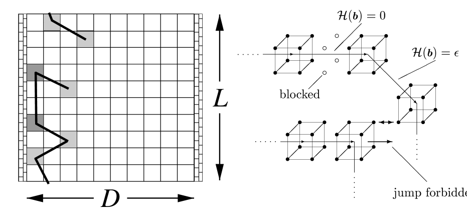
FIG. 1.:

FIG. 2.:

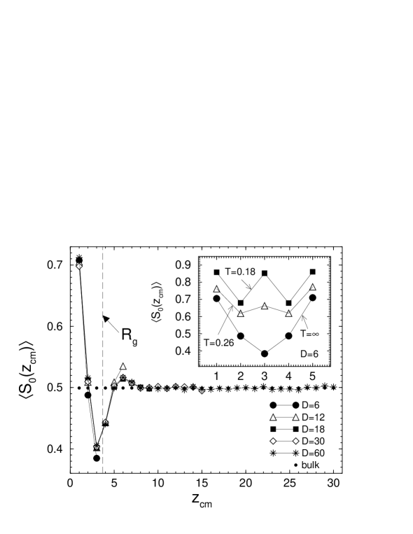
FIG. 3.:

FIG. 4.:

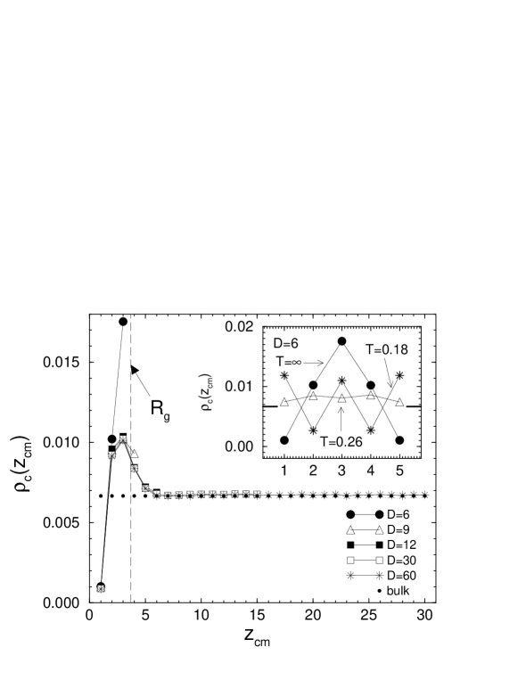
FIG. 5.:

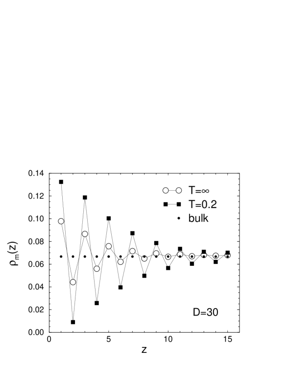
FIG. 6.:

FIG. 7.:

FIG. 8.:

FIG. 9.:

FIG. 10.:

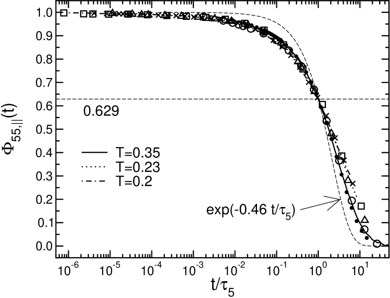
FIG. 11.:

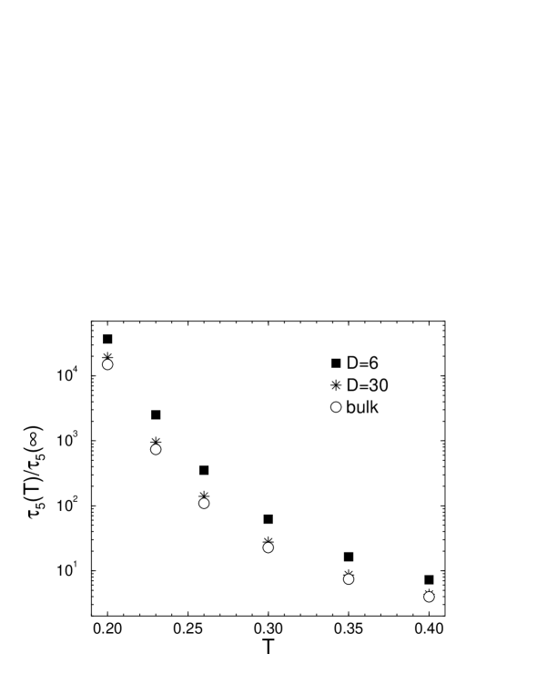
FIG. 12.:

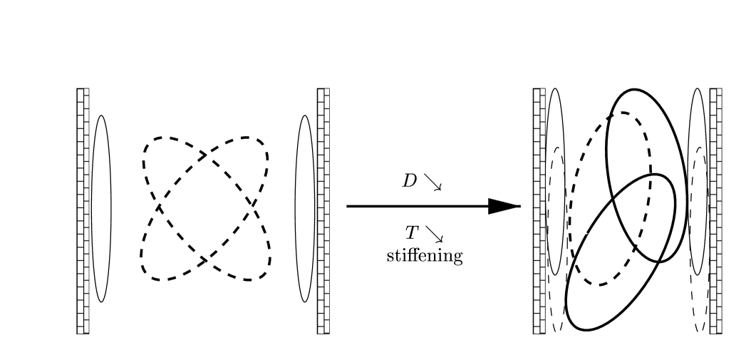
FIG. 13.:

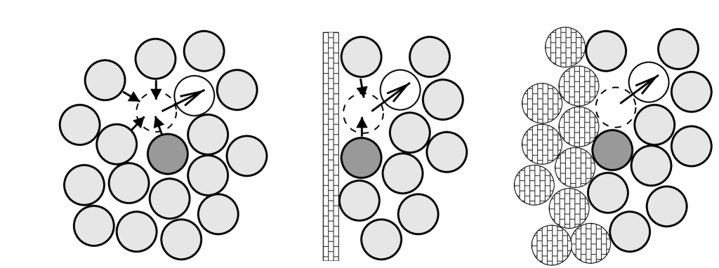
FIG. 14.:

REFERENCES

- [1] Proceedings of the Third International Discussion Meeting on Relaxation in Complex Systems, J. Non–Cryst. 235-237 (1998).
- [2] Proceedings of the International Workshop on Dynamics in Confinement, J. Phys. IV France 10 (2000).
- [3] Proceedings of the ICTP–NIST Conference on Unifying Concepts in Glass Physics, J. Phys.: Condens. Matter 12 (2000).
- [4] W. Götze, J. Phys.: Condens. Matter 11 (1999) A1.
- [5] J. Jäckle, Rep. Progr. Phys. 49 (1986) 171.
- [6] K. Binder and A. Young, Rev. Mod. Phys. 58 (1986) 801.
- [7] H. Fynewever and P. Harrowell, J. Phys.: Condens. Matter 12 (2000) 6305.
- [8] R. Yamamoto and A. Onuki, Phys. Rev. E 58 (1998) 3515.
- [9] B. Doliwa and A. Heuer, J. Phys.: Condens. Matter 11 (1999) A277.
- [10] S.C. Glotzer, V.N. Novikov and T.B. Schrøder, J. Chem. Phys. 112 (2000) 509.
- [11] C. Donati, S.C. Glotzer, P.H. Poole, W. Kob and S.J. Plimpton, Phys. Rev. E 60 (1999) 3107.
- [12] C. Bennemann, C. Donati, J. Baschnagel and S.C. Glotzer, Nature 399 (1999) 246.
- [13] W.K. Kegel and A. van Blaaderen, Science 287 (2000) 290.
- [14] E.R. Weeks, J.C. Crocker, A.C. Levitt, A. Schofield and D.A. Weitz, Science 287 (2000) 627.
- [15] H. Sillescu, J. Non-Cryst. Solids 243 (1999) 243.
- [16] M.D. Ediger, Annu. Rev. Phys. Chem. 51 (2000) 99.
- [17] C.L. Jackson and G.B. McKenna, Chem. Mater. 8 (1996) 2128.
- [18] H. Wendt and R. Richert, J. Phys.: Condens. Matter 11 (1999) A199.
- [19] J. Schüller, R. Richert and E.W. Fischer, Phys. Rev. B 52 (1995) 15232.
- [20] K. Kremer, A. Huwe, M. Arndt, P. Behrens and W. Schwieger, J. Phys.: Condens. Matter 11 (1999) A175.
- [21] G. Barut, P. Pissis, R. Pelster and G. Nimtz, Phys. Rev. Lett. 80 (1998) 3543.
- [22] J.L. Keddie, R.A.L. Jones and R.A. Cory, Europhys. Lett. 27 (1994) 59.
- [23] J.A. Forrest, K. Dalnoki-Veress, J.R. Stevens and J.R. Dutcher, Phys. Rev. Lett. 77 (1996) 2002; ibid. 4108.
- [24] J.A. Forrest, K. Dalnoki-Veress and J.R. Dutcher, Phys. Rev. E 56 (1997) 5705.
- [25] J.A. Forrest, C. Svanberg, K. Révész, M. Rodahl, L.M. Torell and B. Kasemo, Phys. Rev. E 58 (1998) R1226.
- [26] J.A. Forrest and J. Mattsson, Phys. Rev. E 61 (2000) R1226.
- [27] S.H. Anastasiadis, K. Karatosos, G. Vlachos, E. Manias and E.P. Giannelis, Phys. Rev. Lett. 84 (2000) 915.
- [28] D.S. Fryer, P.F. Nealey and J.J. de Pablo, Macromolecules 33 (2000) 6439.
- [29] B. Böddeker and H. Teichler, Phys. Rev. E 59 (1999) 1948.
- [30] K.F. Mansfield and D.N. Theodorou, Macromolecules 24 (1991) 6283.
- [31] Z.T. Németh and H. Löwen, Phys. Rev. E 59 (1999) 6824.
- [32] T. Fehr and H. Löwen, Phys. Rev. E 52 (1995) 4016.
- [33] R. Yamamoto and K. Kim, J. Phys. IV France 10 (2000) Pr7-15.
- [34] P. Scheidler, W. Kob and K. Binder, The Relaxation Dynamics of a Simple Glass Former Confined in a Pore [cond-mat/0003257].
- [35] P. Gallo, M. Rovere, M.A. Ricci, C. Harting and E. Spohr, Europhys. Lett. 49 (2000) 183; P. Gallo, M. Rovere and E. Spohr, Glass Transition and Layering Effects in Confined Water: A Computer Simulation Study [cond-mat/0010147].
- [36] J. Baschnagel and K. Binder, J. Phys. I France 6 (1996) 1271.
- [37] F.W. Starr, T.B. Schrøder and S.C. Glotzer, Effects of a Nano-Sized Filler on the Structure and Dynamics of a Simulated Polymer Melt and the Relationship to Ultra-Thin Films [cond-mat/0007486].
- [38] J. Jäckle, J. Phys. IV France 10 (2000) Pr7-3.
- [39] P.G. de Gennes, Eur. Phys. J. E 2 (2000) 201; commentaries by K. Binder and R.A.L. Jones, ibid., 204, 205; P.G. de Gennes, Glass Transitions of Freely Suspended Polymer Films [cond-mat/0009176].
- [40] L. Bocquet and J.–L. Barrat, Europhys. Lett. 31 (1995) 455.
- [41] S. Büchner and A. Heuer, Phys. Rev. E 60 (1999) 6507.
- [42] K. Kim and R. Yamamoto, Phys. Rev. E 61 (2000) R41.
- [43] J. Jäckle and H. Kawai, Molecular Dynamics Study of the Dependence of Self-Diffusion on System Size in a Dense Binary Liquid of Hard Spheres, submitted to Physica A.
- [44] J. Horbach, W. Kob, K. Binder and C.A. Angell, Phys. Rev. E 54 (1996) R5897.
- [45] J. Horbach and W. Kob, Phil. Mag. B 79 (1999) 1981.
- [46] P. Scheidler, W. Kob and K. Binder, J. Phys. IV France 10 (2000) Pr7-33.
- [47] P. Doruker and W.L. Mattice, Macromolecules 32 (1999) 194.
- [48] J.A. Torres, P.F. Nealy and J.J. de Pablo, Phys. Rev. Lett. 85 (2000) 3221.
- [49] J. Baschnagel, C. Mischler and K. Binder, J. Phys. IV France 10 (200) Pr7-9.
- [50] F. Varnik, J. Baschnagel and K. Binder, J. Phys. IV France 10 (2000) Pr7-239.
- [51] J.A. Forrest and R.A.L. Jones, in A. Karim and S. Kumar (Eds.), Polymer Surfaces, Interfaces and Thin Films (World Scientific, Singapore, 2000), pp. 251–294.
- [52] J.A. Forrest and K. Dalnoki–Veress, The Glass Transition in Thin Polymer Films, preprint.
- [53] I. Carmesin and K. Kremer, Macromolecules 21 (1988) 2819.
- [54] H.-P. Deutsch and K. Binder, J. Chem. Phys. 94 (1991) 2294.
- [55] H.-P. Wittmann and K. Kremer, Comp. Phys. Comm. 61 (1990) 309; H.-P. Wittmann and K. Kremer, Comp. Phys. Comm. 71 (1992) 343.
- [56] A.D. Sokal, in K. Binder (Ed.), Monte Carlo and Molecular Dynamics Simulations in Polymer Science (Oxford University Press, New York, 1995), pp. 47–124.
- [57] K. Binder, in K. Binder (Ed.), Monte Carlo and Molecular Dynamics Simulations in Polymer Science (Oxford University Press, New York, 1995), pp. 3–46.
- [58] K. Kremer and K. Binder, Comp. Phys. Rep. 7 (1988) 259.
- [59] W. Paul, K. Binder, D.W. Heermann and K. Kremer, J. Phys. II 1 (1991) 37; W. Paul, K. Binder, D.W. Heermann and K. Kremer, J. Chem. Phys. 95 (1991) 7726.
- [60] J. Baschnagel, K. Binder, P. Doruker, A.A. Gusev, O. Hahn, K. Kremer, W.L. Mattice, F. Müller–Plathe, M. Murat, W. Paul, S. Santos, U.W. Suter, V. Tries, Adv. Polym. Sci. 152 (2000) 41.
- [61] J. Baschnagel, in M.R. Tant and A.J. Hill (Eds.), Structure and Properties of Glassy Polymers, (ACS Symposium Series No. 710, American Chemical Society, Washington, DC, 1998), pp. 53–77.
- [62] W. Paul and J. Baschnagel, in K. Binder (Ed.) Monte Carlo and Molecular Dynamics Simulations in Polymer Science (Oxford University Press, New York, 1995), pp. 307–355.
- [63] J. Baschnagel, K. Binder and H.-P. Wittmann, J. Phys.: Condens. Matter 5 (1993) 1597.
- [64] J.H. Gibbs and E.A. Di Marzio, J. Chem. Phys. 28 (1958) 373.
- [65] G.B. McKenna, in C. Booth and C. Price, Comprehensive Polymer Science, Vol. 2 (Pergamon Press, New York, 1989), pp. 311–362.
- [66] M. Wolfgardt, J. Baschnagel, W. Paul and K. Binder, Phys. Rev. E 54 (1996) 1535; J. Baschnagel, M. Wolfgardt, W. Paul and K. Binder, J .Res. Natl. Inst. Stand. Technol. 102 (1997) 135.
- [67] K. Binder and D.W. Heermann, Monte Carlo Simulation in Statistical Physics: An Introduction (Springer, Berlin-Heidelberg, 1997).
- [68] M. Doi and S.F. Edwards, Theory of Polymer Dynamics (Clarendon Press, Oxford, 1986).
- [69] B. Dünweg, M. Stevens and K. Kremer, in K. Binder (Ed.), Monte Carlo and Molecular Dynamics Simulations in Polymer Science (Oxford University Press, New York, 1995), pp. 125–193.
- [70] K. Binder and W. Paul, J. Polym. Sci. B 35 (1997) 1.
- [71] M. Wolfgardt, J. Baschnagel and K. Binder, J. Phys. II (France) 5 (1995) 1035.
- [72] V. Tries, W. Paul, J. Baschnagel and K. Binder, J. Chem. Phys. 106 (1997) 738.
- [73] M. Müller, J. Wittmer and J.-L. Barrat, On two intrinsic length scales in polymer physics: topological constraints vs. entanglement length, submitted to Europhys. Lett. [cond-mat/0006464].
- [74] T. Kreer, J. Baschnagel, M. Müller and K. Binder, Monte Carlo Simulation of Long Chain Polymer Melts: Crossover from Rouse to Reptation Dynamics, submitted to Macromolecules [cond-mat/0008355].
- [75] G.J. Fleer, M.A. Cohen Stuart, J.M.H.M. Scheutjens, T. Cosgrove and B. Vincent, Polymers at Interfaces (Chapman & Hall, London, 1993).
- [76] I.C. Sanchez (Ed.), Physics of Polymer Surfaces and Interfaces (Butterworth-Heinemann, Boston, 1992).
- [77] J.B. Hooper, J.D. McCoy and J.G. Curro, J. Chem. Phys. 112 (2000) 3090.
- [78] J.B. Hooper, M.T. Pileggi, J.D. McCoy, J.G. Curro and J.D. Weinhold, J. Chem. Phys. 112 (2000) 3094.
- [79] M. Müller and L. Gonzalez MacDonald, Macromolecules 33 (2000) 3902.
- [80] A. Yethiraj, J. Chem. Phys. 109 (1998) 3269.
- [81] S. Sen, J.M. Cohen, J.D. McCoy and J.G. Curro, J. Chem. Phys. 101 (1994) 9010.
- [82] S. Phan, E. Kierlik, M.L. Rosinberg, A. Yethiraj and R. Dickman, J. Chem. Phys. 102 (1995) 2141.
- [83] A. Yethiraj, S. Kumar, A. Hariharan and K.S. Schweizer, J. Chem. Phys. 100 (1994) 4691.
- [84] P.K. Brazhnik, K. Freed and H. Tang, J. Chem. Phys. 101 (1994) 9143.
- [85] C. E. Woodward and A. Yethiraj, J. Chem. Phys. 100 (1994) 3181.
- [86] K. P. Walley, K.S. Schweizer J. Peanasky, L. Cai and S. Granick, J. Chem. Phys. 100 (1994) 3361.
- [87] E. Kierlik and M.L. Rosinberg, J. Chem. Phys. 100 (1994) 1716.
- [88] D.N. Theodorou, Macromolecules 21 (1988) 1391; ibid. 21 (1988) 1400.
- [89] I. A. Bitsanis and G. ten Brinke, J. Chem. Phys. 99 (1993) 3100.
- [90] G. ten Brinke, D. Ausserre and G. Hadziioannou, J. Chem. Phys. 89 (1988) 4374.
- [91] T. Pakula, J. Chem. Phys. 95 (1991) 4685.
- [92] J.-S. Wang and K. Binder, J. Phys. I France 1 (1991) 1583.
- [93] J. Baschnagel and K. Binder, Macromolecules 28 (1995) 6808.
- [94] J. Baschnagel and K. Binder, Macromol. Theory Simul. 5 (1996) 417.
- [95] R.S. Pai-Panandiker, J.R. Dorgan and T. Pakula, Macromolecules 30 (1997) 6348.
- [96] Do Y. Yoon, M. Vacatello and G. D. Smith, in K. Binder (Ed.), Monte Carlo and Molecular Dynamics Simulations in Polymer Science, (Oxford University Press, New York, 1995), pp. 433–475.
- [97] I. A. Bitsanis and G. Hadziioannou, J. Chem. Phys. 92 (1990) 3827.
- [98] R.G. Winkler, T. Matsuda and Do Y. Yoon, J. Chem. Phys. 98 (1993) 729.
- [99] M. Vacatello, Macromol. Theory Simul. 3 (1994) 325.
- [100] S. K. Kumar, M. Vacatello and Do Y. Yoon, Macromolecules 23 (1990) 2189.
- [101] R. Dickman, J. Chem. Phys. 96 (1992) 1516.
- [102] A. Yethiraj, J. Chem. Phys. 101 (1994) 2489.
- [103] J. Kraus, P. Müller-Buschbaum, T. Kuhlmann, D.W. Schubert and M. Stamm, Europhys. Lett. 49, 210 (2000).
- [104] R.L. Jones, S.K. Kumar, D.L. Ho, R.M. Briber and T.P. Russell, Nature 400 (2000) 146.
- [105] J.A. Aronovitz and D.R. Nelson, J. Physique 47 (1986) 1445.
- [106] K. Šolc and W.H. Stockmayer, J. Chem. Phys. 54 (1971) 2756; K. Šolc, J. Chem. Phys. 55 (1971) 335.
- [107] J.W. Cannon, J.A. Aronovitz, P. Goldbart, J. Phys. I 1 (1991) 629.
- [108] H.W.H.M. Janszen, T.A. Tervoort, P. Cifra, Macromolecules 29 (1996) 5678.
- [109] F. Eurich, P. Maass, Soft Ellipsoid Model for Gaussian Polymer Chains, cond-mat/0008425.
- [110] J. Rudnick and G. Gaspari, J. Phys. A: Math. Gen. 19 (1986) L191.
- [111] A. Yethiraj and C. K. Hall, Macromolecules 23 (1990) 1865.
- [112] J. Baschnagel, K. Binder and A. Milchev, in A. Karim and S. Kumar (Eds.), Polymer Surfaces, Interfaces and Thin Films (World Scientific, Singapore, 2000), pp. 1–49.
- [113] M. Vacatello, D. Y. Yoon and B. C. Laskowski, J. Chem. Phys. 93 (1990) 779.
- [114] J. Baschnagel and K. Binder, Mat. Res. Soc. Symp. Proc. 543 (1999) 157.
- [115] F. Schmid, J. Chem. Phys. 104 (1996) 9191.
- [116] J. Baschnagel and K. Binder, Physica A 204 (1994) 47.
- [117] W. Götze, in J.P. Hansen, D. Levesque and J. Zinn-Justin (Eds.), Liquids, Freezing and the Glass Transition, Part 1 (North-Holland, Amsterdam, 1990), pp. 287–503.
- [118] W. Götze and L. Sjögren, Rep. Prog. Phys. 55 (1992) 241.
- [119] W. Götze and L. Sjögren, in S. Yip and P. Nelson (Eds.), Trans. Theory Stat. Phys. 24, 801 (1995).
- [120] J. Baschnagel, Phys. Rev. B 49 (1994) 135.
- [121] J. Baschnagel and M. Fuchs, J. Phys.: Condens. Matter 7 (1995) 6761. (1995).
- [122] P.H. Verdier, J. Chem. Phys. 45 (1966) 2118.
- [123] K. Okun, M. Wolfgardt, J. Baschnagel and K Binder, Macromolecules 30 (1997) 3075.
- [124] C. Bennemann, J. Baschnagel, W. Paul, K. Binder, Comp. Theo. Poly. Sci. 9 (1999) 217.
- [125] K.L. Ngai, A.K. Rizos, D.J. Plazek, J. Non-Cryst. Solids 235–237 (1998) 435.
- [126] S. Yip and P. Nelson (Eds.), Trans. Theory Stat. Phys. 24, No. 6–8 (1995).
- [127] W. Kob, in D. Stauffer (Ed.), Annual Reviews of Computational Physics Vol. 3, (World Scientific, Singapore, 1995), pp 1–43.
- [128] W. Kob, J. Phys.: Condens. Matter 11 (1999) R85.
- [129] J.–L. Barrat and L. Bocquet, Faraday Discuss. 112 (1999) 119.
- [130] Y. Alméras, J.–L. Barrat and L. Bocquet, J. Phys. IV France 10 (2000) Pr7-27.
- [131] J.L. Keddie, R.A.L. Jones and R.A. Cory, Faraday Discuss. 98 (1994) 219.
- [132] M. Arndt, R. Stannarius, H. Groothues, E. Hempel and F. Kremer, Phys. Rev. Lett. 79 (1997) 2077.