Spin-dependent transport in a Luttinger liquid

Abstract

We develop a detailed theory for spin transport in a one-dimensional quantum wire described by Luttinger liquid theory. A hydrodynamic description for the quantum wire is supplemented by boundary conditions taking into account the exchange coupling between the magnetization of ferromagnetic reservoirs and the boundary magnetization in the wire. Spin-charge separation is shown to imply drastic and qualitative consequences for spin-dependent transport. In particular, the spin accumulation effect is quenched except for fine-tuned parameter regimes. We propose several feasible setups involving an external magnetic field to detect this phenomenon in transport experiments on single-wall carbon nanotubes. In addition, electron-electron backscattering processes, which do not have an important effect on thermodynamic properties or charge transport, are shown to modify spin-dependent transport through long quantum wires in a crucial way.

I Introduction

Spin-polarized transport represents a new branch of mesoscopic physics, in which both the charge and spin of the electron are actively manipulated.[1, 2, 3, 4, 5] In different setups, the spin may be employed as information storage or transport element, where the advantage over charge transport stems from the very long spin lifetimes in many materials, and the smallness of the dissipated power. These advantages have already resulted in many technological applications, and among the most popular future perpectives of spintronics is the field of quantum computation.[6] Spin-dependent transport also offers novel insights into fundamental physics. In this paper we shall address in detail how spin transport proceeds in strongly interacting non-Fermi liquid metals, taking the behavior of one-dimensional (1D) metals as a paradigm in which electron-electron interactions lead to a breakdown of Fermi liquid theory. The 1D non-Fermi liquid behavior is often described by Luttinger liquid (LL) theory.[7]

The primary motivation for this study comes from recent transport experiments[8] on carbon nanotubes,[9] which have demonstrated the breakdown of Fermi liquid theory in these nearly ideal 1D quantum wires (QWs). In fact, when studying charge transport in single-wall nanotubes (SWNTs), the observed power-law behaviors in the tunneling density of states are consistent with their theoretical description[10] in terms of a LL. The LL describes metals in the 1D limit where only one or very few bands intersect the Fermi energy. This non-Fermi liquid exhibits fractionalization of electrons into novel quasiparticles, comprising a diverse set carrying spin separately from charge, and charge in fractions of the electron charge $e$.[11] Furthermore, the LL is the simplest model showing the remarkable phenomenon of spin-charge separation which has been postulated by many to underly the cuprate superconductors.[12, 13, 14, 15] In a LL, spin and charge degrees of freedom are completely decoupled, and moreover characterized by different velocities. As Landau quasiparticles are unstable, an electron will spontaneously decay into charge and spin density wave packets which then propagate with different velocities. Thereby a spatial separation of spin and charge of the electron results. Unfortunately, this hallmark behavior of strongly correlated 1D fermions remains to be observed experimentally (at least in an unambiguously accepted way). Elaborating on our short paper,[16] we propose several feasible setups that would allow to unambiguously detect spin-charge separation via spin transport experiments on an individual SWNT. For related but rather different proposals to detect spin-charge separation in a LL via spin transport, see also Refs. [17] and [18].

As will be described at length below, this can be achieved by attaching ferromagnetic leads to the QW, and possibly an additional magnetic field, see Fig. 1. For simplicity, identical contact parameters are assumed below, with straightforward generalization possible. By measuring the variations of the current-voltage $(I-V)$ characteristics with either the angle $\theta$ between the ferromagnetic magnetizations in the leads, or the magnetic field $\vec{B}$, one can indeed directly probe spin-charge separation. A related spin-transport experiment has been carried out recently for multi-wall nanotubes, where the angle $\theta$ was fixed to either zero or $\theta=\pi$.[19] The experiment proposed here for SWNTs should either allow for arbitrary $\theta$, or employ an additional magnetic field. We note that spin transport in such a setup is well understood for Fermi liquids. In particular, the $I-V$ characteristics (including a magnetic field) have been computed recently using a semiclassical description.[20]

In our theory, we assume that tunneling across the two contacts proceeds incoherently, i.e., the length $L$ of the QW must be longer than either the thermal length scale $\hbar v/k_{B}T$ or the scale $\hbar v/eV$ set by the applied voltage $V$. We then consider in general systems composed of 1D interacting quantum wires and bulk ferromagnets. With the exception of Sec. VI, where the additional flavor degree of freedom present in SWNTs will be addressed, we focus on single-mode QWs.

Another interesting aspect of spin transport concerns the role of electron-electron backscattering interactions. In a spin-$\frac{1}{2}$ QW, these interactions are (marginally) irrelevant under the renormalization group (RG) flow, and therefore only cause a renormalization of interaction parameters in the low-energy LL theory.[7] However, this essentially thermodynamic (equilibrium) argument must be re-examined when dealing with spin transport. In fact, such interactions, despite being irrelevant, can result in nonlinear and sometimes dramatic effects, e.g., a non-sinusoidal oscillatory $I-V$ characteristics.

The structure of this paper is as follows. In Sec. II, we introduce the basic model and outline the computation of the non-equilibrium spin current. In Sec. III, the physics arising at a contact between a ferromagnetic reservoir and a Luttinger liquid is addressed at length. Two processes are shown to be of importance, namely electron tunneling and boundary exchange. Exchange leads to novel conformally-invariant boundary conditions which are derived here. In Sec. IV, a hydrodynamic description of spin transport in the 1D QW is developed. In Sec. V, we derive the $I-V$ characteristics in a magnetic field for the simplest spin transport device, see Fig. 1, first for a short-to-intermediate length of the QW. Under the latter condition, backscattering can be neglected. The effects of backscattering are then addressed in detail in Secs. V C and V D, where we focus on zero magnetic field for clarity. Finally, several extensions and possible concerns are addressed in Sec. VI. We conclude in Sec. VII by discussing an analogy to ballistic superconductor-normal-superconductor (SNS) junctions, summarizing some open questions and providing an outlook. Details of our calculations in Sec. V can be found in three appendices. In intermediate steps of the calculations, we put $e=\hbar=1$, but restore units in experimentally relevant results.

II Model and Formulation

The low-energy description of a single-mode QW is remarkably universal,[7] and a sufficient Hamiltonian for our purposes is

$$H_{\rm QW}=\int_{0}^{L}\!\!\!\!dx\,\left\{-i\psi^{\dagger}v\tau^{z}\partial_{x}\psi^{\vphantom{\dagger}}+u\left(\psi^{\dagger}\psi^{\vphantom{\dagger}}\right)^{2}\right\}\;,$$ (1)

where $\psi=\psi_{a\alpha}$ is a four-component spinor. Here $a=R/L$ indexes the chirality that differentiates right- and left-moving modes, and $\alpha=\uparrow/\downarrow$ indexes the spin. We suppress the indices whenever possible, employing Pauli matrices $\vec{\tau}$ and $\vec{\sigma}$ acting in the chirality and spin spaces, respectively. Furthermore, $v$ denotes the Fermi velocity, or, more generally, the spin velocity of the interacting theory. If the QW is isolated, the zero-current condition at the endpoints requires to impose the boundary conditions $\psi_{R}(0)=\psi_{L}(0)$ and $\psi_{R}(L)=\psi_{L}(L)$. Only the forward-scattering interaction $u$ is kept in Eq. (1). Alternatively, we will use the exponent $\alpha>0$ for tunneling into the end of the LL, e.g., at $x=0$, as a measure of the interaction strength. Eq. (1) is not completely general. It contains two parameters, $v$ and $u$, while a general single-mode LL has three parameters: a charge velocity $v_{c}$, a spin velocity $v$, and a dimensionless “Luttinger parameter”, often denoted $K_{\rho}$ or $g$, where $\alpha=(K_{\rho}^{-1}-1)/2$. In Eq. (1), we have assumed full (Galilean) translational invariance, leading to $K_{\rho}=v/v_{c}$. This relation is expected to be well-satisfied in many experimentally relevant QWs, and moreover the manipulations to follow relax this condition and thus can be applied even when $K_{\rho}\neq v/v_{c}$.

In some circumstances, Eq. (1) should be supplemented by the electron-electron backscattering interaction,

$$H_{\rm bs}=-bv\int dx\vec{J}_{L}\cdot\vec{J}_{R}\;,$$ (2)

with the chiral spin currents

$$\vec{J}_{R/L}(x)=\frac{1}{2}:\psi^{\dagger}_{R/L}(x)\vec{\sigma}\psi^{\vphantom{\dagger}}_{R/L}(x):\;,$$ (3)

where the colons denote normal ordering. These chiral spin currents obey Kac-Moody commutation relations ($\mu,\nu=x,y,z$),

$$[J_{L/R}^{\mu}(x),J_{L/R}^{\nu}(x^{\prime})] = \pm i\delta^{\prime}(x-x^{\prime})\delta^{\mu\nu}$$ (4)

$$+ i\epsilon^{\mu\nu\lambda}J_{L/R}^{\lambda}(x)\delta(x-x^{\prime})\;,$$ (5)

where the $+$ ($-$) sign is associated with the $L$ ($R$) current. We note that in a spin-$1/2$ QW, the backscattering interaction (2) is marginally irrelevant in the RG sense, and hence can be neglected at low energies in many equilibrium properties. In a SWNT, the generalization of $H_{\rm bs}$ causes exponentially small gaps that can be neglected at not too low energies. Furthermore, the dimensionless backscattering coupling constant $b$ is generally small and scales as $1/R$ with the tube radius $R$. Importantly, as will be discussed below in detail, a precession effect encoded in Eq. (2) is crucial for understanding spin transport in long QWs.

For energies well below the electronic bandwidth $D$, a ferromagnetic (FM) lead can be described using an effectively non-interacting Stoner-like picture[21] with a constant density of states. It is then sufficient to employ a non-interacting 1D model, e.g., for the left lead ($x<0$),

$$H_{\rm FM}=\sum_{s=\pm 1}\int_{-\infty}^{0}\!\!\!\!dx\,f^{\dagger}\left(-iv_{s}\hat{u}_{s}\tau^{z}\partial_{x}\right)f^{\vphantom{\dagger}}\;,$$ (6)

where $f$ is again a four-component spinor. Comparing to Eq. (1), different spin quantization axes have been used, and therefore the projection operator

$$\hat{u}_{s}=(1\pm\hat{m}\cdot\vec{\sigma})/2$$ (7)

projecting the spin quantization axis of the QW onto the magnetization $\hat{m}$ is needed. This description of the semi-infinite lead must be supplemented by an appropriate boundary condition, $f_{R}(0)=f_{L}(0)$. In Eq. (6), the two Fermi velocities $v_{\pm}$ parameterize the different densities of states, $\rho_{s}=1/(2\pi v_{s})$, for the majority and minority carriers. Following Ref. [20], we choose a suitable rescaling of the $f$ operators to set $v_{+}=v_{-}=1$, thereby incorporating the difference in the density of states into a redefinition of the hopping matrix elements, $t_{s}\rightarrow t_{s}/\rho_{s}$, employed in the tunneling Hamiltonian, see Eq. (8) below. Formally this is done by choosing eigenstates $f_{s}$ of $\hat{m}\cdot\vec{\sigma}$ with eigenvalue $s=\pm$, and then rescaling $f_{s}(x)\rightarrow v_{s}^{-1}f_{s}(x/v_{s})$, the spatial rescaling being allowed because the different spin polarizations are non-interacting and tunneling acts only at $x=0$.

The LLs and FMs in question will be considered coupled by low-conductance contacts with identical properties. Processes in which electrons are transferred across such a contact can be described by the tunneling Hamiltonian $H_{\rm tun}$. Provided this contact occurs at one of the ends of the LL, say, at $x=0$, this has the form

$$H_{\rm tun}=F^{\dagger}W\Psi^{\vphantom{\dagger}}+\Psi^{\dagger}W^{\dagger}F^{\vphantom{\dagger}}\;,$$ (8)

where $F=f(0^{-})$ and $\Psi=\psi(0^{+})$ are Fermion annihilation operators at the ends of the FM and QW, respectively. The 2$\times$2 tunneling matrix $W$ reads with Eq. (7),

$$W=\sum_{s=\pm 1}t_{s}\hat{u}_{s}\;.$$ (9)

Using the spin-dependent hopping matrix elements $t_{s}$, we may define spin-dependent conductances $G_{s}=(e^{2}/h)|t_{s}|^{2}$, or, alternatively, the contact parameters

$$G=G_{\uparrow}+G_{\downarrow}\;,\quad P=(G_{\uparrow}-G_{\downarrow})/G\;.$$ (10)

Here $G$ is the total conductance associated with the contact. In a slight abuse of terminology, we call $P$ the polarization. The polarization satisfies $0\leq P\leq 1$, and in fact represents the asymmetry between the local tunneling density of states of the majority and minority carriers of the ferromagnet. Hence $P$ is not a bulk property, and depends upon the detailed nature of the FM-QW contact. In the experiment of Ref. [19], application of our theoretical results, in particular Eq. (86) – which differs slightly from the theory used in Ref. [19] – gives a value of $P=0.3$ for a multi-wall NT to FM (cobalt) contact at $T=4.2K$.

From Eq. (8), one may deduce the spin current, defined by

$$\vec{J}^{\rm tun}={\partial\over{\partial t}}\left.\left(\int\!dx\,\vec{M}\right)\right|_{\rm tun}\;,$$ (11)

where the magnetization density in the QW is

$$\vec{M}=\vec{J}_{R}+\vec{J}_{L}\;.$$ (12)

Using the continuity equation in the absence of backscattering interactions, $b=0$, the steady-state current is thus

$$\vec{J}=v(\vec{J}_{R}-\vec{J}_{L})\;.$$ (13)

Then the tunneling current is

$$\vec{J}_{\rm tun}={i\over 2}\left(F^{\dagger}W\vec{\sigma}\Psi^{\vphantom{\dagger}}-\Psi^{\dagger}\vec{\sigma}\,W^{\dagger}F^{\vphantom{\dagger}}\right)\;.$$ (14)

Of course, a formula similar to Eq. (14) obtains for the charge current across the contact,

$$I=i\left(F^{\dagger}W\Psi^{\vphantom{\dagger}}-\Psi^{\dagger}W^{\dagger}F^{\vphantom{\dagger}}\right)\;.$$ (15)

In addition to the tunnel coupling in Eq. (8), the FM magnetization and the LL boundary magnetization can be coupled by a pure exchange term,

$$H_{\rm ex}=-K\hat{m}\cdot\Psi^{\dagger}{\vec{\sigma}\over 2}\Psi^{\vphantom{\dagger}}\;.$$ (16)

Even if in a microscopic formulation no bare exchange coupling $K$ is present, it will be generated in the low-energy effective Hamiltonian since tunneling causes virtual processes corresponding to exchange, see below and Ref. [22].

To study transport, we must formulate the non-equilibrium dynamics of the system. This formulation is more subtle than in conventional charge transport, due to the complications arising from the non-commuting nature of spin. We therefore proceed carefully along the lines of a Keldysh approach. For concreteness, we specialize for the moment to a semi-infinite LL contacted at $x=0$. Consider an initial system composed of two decoupled pieces, described by the Hamiltonian $H_{0}=H_{\rm FM}+H_{\rm QW}$. The ferromagnetic part, governed by $H_{\rm FM}$, is polarized along direction $\hat{m}$, and located at $x<0$. The wire, located at $x>0$, is governed by $H_{\rm QW}$, which is assumed $SU(2)$ invariant. The latter condition guarantees the existence of a continuity equation for the spin density and current. Similarly, charge conservation implies a continuity equation for charge density and current. At $t=-\infty$, we assume that each half is at quasi-equilibrium at its own chemical potential, $\mu_{\rm FM}$ and $\mu_{\rm QW}$. Similarly, we assume that the LL supports a quasi-equilibrium magnetization, which can be described by a grand canonical distribution with a “spin chemical potential” $\vec{h}$. We stress that neither $\mu_{\rm QW}$ nor $\vec{h}$ are physical potentials, such as electrostatic or Zeeman fields, but rather characterize the initial non-equilibrium distribution. Then we adiabatically turn on the contact perturbation $H^{\prime}=H_{\rm tun}+H_{\rm ex}$,

$$H(t)=H_{0}+e^{\delta t}H^{\prime}\;,$$ (17)

where $\delta\rightarrow 0^{+}$ is an infinitesimal inverse time-scale controlling the slow turning on of the contact interaction.

The above formulation is rather rigorous, but has the limitation of being formulated to treat both the tunneling and boundary exchange terms as perturbations. In practice, this is appropriate in the low-conductance limit, since the boundary exchange is generally determined by virtual tunneling processes, and is hence small. However, it is useful theoretically to contemplate a situation in which the tunneling is small but the boundary exchange is not. In such a case, it appears natural to include $H_{\rm ex}$ into $H_{0}$ rather than in $H^{\prime}$. This raises difficult conceptual issues, since $H_{\rm ex}$ does not commute with the total spin of the LL, and hence renders its magnetization uncertain in directions perpendicular to $\hat{m}$. On physical grounds, however, we expect that, because $H_{\rm ex}$ transfers spin into/out of the LL only at the boundary, sense can be made of the bulk spin chemical potential in the limit of a semi-infinite LL. This is fairly clear from the following thought experiment: imagine preparing the LL with zero tunneling and zero boundary exchange in a state with a non-zero magnetization density not parallel to $\hat{m}$. Then, if $H_{\rm ex}$ is turned on at some time, its effect will be to scatter left-moving electrons into right-moving ones upon their reaching $x=0$, changing their spin orientation in the process. If the LL is semi-infinite, however, it would take an infinite amount of time to modify the mean magnetization of the LL in this way. Instead, one expects a steady-state to be established, generally with a time-independent spin current. Moreover, for a finite but long LL, so long as there are some inelastic processes deep in the LL that can equilibrate the returning electrons, one expects that an equilibrium state will be established which has a mean magnetization very close to that before turning on the boundary exchange. In fact, a scattering approach of this type can be directly implemented using bosonization methods, and will be discussed analytically in Sec. III B. Alternatively, $H_{\rm ex}$ can be incorporated directly into $H_{0}$, but in this case, care must be taken to ensure that $\vec{h}$ is coupled only to the magnetization outside a neighborhood of the boundary. For the moment, we simply use the above discussion as motivation to incorporate $H_{\rm ex}$ into $H_{0}$.

We are interested in the properties of the system at time $t=0$, when a steady-state transport of charge and spin between the two systems has been achieved. Then we can formally calculate the expectation value of any operator at this time:

$$\langle{\cal O}(0)\rangle = {1\over Z}{\rm Tr}\,\bigg{[}e^{-\beta(H_{0}-\Lambda)}{\cal T}\exp\left(i\int_{-\infty}^{0}dtH(t)\right){\cal O}$$ (19)

$$\times{\cal T}\exp\left(-i\int_{-\infty}^{0}dtH(t)\right)\bigg{]}\;,$$

where ${\cal T}$ denotes time ordering and

$$\Lambda=\mu_{\rm FM}N_{\rm FM}+\mu_{\rm QW}N_{\rm QW}+\vec{h}\cdot\vec{S}_{\rm QW}^{\rm tot}\;.$$ (20)

It will be most convenient to choose the zero of energy in $H$ such that $\mu_{\rm FM}=\mu_{\rm QW}=h=0$ in equilibrium, i.e., for zero applied voltage.

Expanding out the time-ordered exponential, one obtains to lowest order

$$\langle{\cal O}\rangle=-i\int_{-\infty}^{0}\!dt\,{1\over Z}{\rm Tr}\,\left(e^{-\beta\tilde{H}_{0}}\left[{\cal O},H^{\prime}(t)\right]\right)e^{\delta t}\;,$$ (21)

where $\tilde{H}_{0}=H_{0}-\Lambda$ and $H^{\prime}(t)=e^{iH_{0}t}H^{\prime}e^{-iH_{0}t}$. Owing to the factor of $\Lambda$ in the Boltzmann weight, not present in the time evolution of $H^{\prime}(t)$, this is a non-equilibrium expectation value. We can cast it into a more equilibrium form by writing $H_{0}=\tilde{H}_{0}+\Lambda$. Then

$$H^{\prime}(t)=e^{i\tilde{H}_{0}t}\left(e^{i\Lambda t}H^{\prime}e^{-i\Lambda t}\right)e^{-i\tilde{H}_{0}t}\;.$$ (22)

Equation (22) has the form of the time-evolution of the operator in the brackets evolved by the “non-equilibrium” Hamiltonian $\tilde{H}_{0}$, which is the same as is used in the Boltzmann weight in Eq. (21). Equation (21) can be rewritten in the slightly more suggestive form,

$$\langle{\cal O}\rangle=-i\int_{-\infty}^{0}\!dt\,e^{\delta t}\left\langle\left[{\cal O},H^{\prime}_{\Lambda}(t)\right]\right\rangle_{\tilde{H}_{0}}\;,$$ (23)

where $H^{\prime}_{\Lambda}$ indicates the modified operator

$$H^{\prime}_{\Lambda}=e^{i\Lambda t}H^{\prime}e^{-i\Lambda t}\;,$$ (24)

which evolves according to the fictitious equilibrium time evolution dictated by $\tilde{H}_{0}$. The subscript $\tilde{H}_{0}$ on the expectation value indicates that it is a standard equilibrium average with respect to the Hamiltonian $\tilde{H}_{0}$, in which the argument of the Fermion fields indicates standard Heisenberg picture time dependence using $\tilde{H}_{0}$,

$$\langle{\cal O}_{1}\cdots{\cal O}_{n}\rangle_{\tilde{H}_{0}} = {1\over Z}{\rm Tr}\,\left(e^{-\beta\tilde{H}_{0}}{\cal O}_{1}\cdots{\cal O}_{n}\right)\;,$$

$${\cal O}(t) = e^{i\tilde{H}_{0}t}{\cal O}e^{-i\tilde{H}_{0}t}\;.$$

Thereby we can express an intrinsically non-equilibrium property of the system with Hamiltonian $H_{0}$ in terms of a fictitious equilibrium average with respect to the shifted Hamiltonian $\tilde{H}_{0}$.

III Contacts

In this section, we analyze in detail the physics of a single contact between a FM lead and a semi-infinite LL (taken at $x=0$). We expect that the results apply to finite-length LLs longer than the thermal length $v/k_{B}T$ beyond which transport is incoherent.

A End contacts: Boundary operators

We first study the properties of the contact in equilibrium from the RG point of view. It is helpful to view both $H_{\rm tun}$ and $H_{\rm ex}$ as perturbations to a decoupled fixed point described by $H_{0}$. Standard arguments give the scaling dimension of both $t_{s}$ and $K$,

$$\Delta_{t_{s}}=1+\alpha/2\;,\quad\Delta_{K}=1\;.$$ (25)

The scaling dimension $\Delta_{K}$ is not renormalized due to spin-charge separation in the QW. A simple calculation then gives the RG scaling equations

$$\partial_{\ell}|t_{s}|^{2}(\ell)=-\alpha|t_{s}|^{2}\;,\qquad\partial_{\ell}K(\ell)=c\left(|t_{\uparrow}|^{2}-|t_{\downarrow}|^{2}\right)\;,$$ (26)

where $\ell=\ln(D/E)$ is the standard RG flow parameter, and $c$ denotes a non-universal constant. Note that $K$ is renormalized by the hopping matrix elements, but the converse does not occur. The most important property of Eq. (26) is that while the tunneling is irrelevant for $\alpha>0$, the exchange coupling $K$ between the LL and FM is exactly marginal.

Following the RG flow from the ultraviolet cutoff $D$ down to energy $E\approx{\rm max}(k_{B}T,eV)\ll D$, we find $|t_{s}|^{2}(E)=|t_{s}|^{2}(E/D)^{\alpha}$, and

$$K(E)=K+\alpha^{-1}cGP[1-(E/D)^{\alpha}]\gg|t_{s}|^{2}(E)\;.$$ (27)

Therefore the effective exchange coupling $K(E)$ does not pick up the $(E/D)^{\alpha}$ suppression factor, and generally is much larger than the effective hopping $t_{s}(E)$, regardless of the microscopic “bare” values of these couplings. Parenthetically, we note that the non-interacting limit, $\alpha\to 0$, is not correctly handled by the simple RG equations (26), as this limit involves additional marginal operators. In fact, for $\alpha\to 0$, not logarithmic dependencies [as predicted by Eq. (27)] but instead a principal parts prescription emerges.

Since the exchange coupling is exactly marginal and the tunneling irrelevant, solving the problem for zero tunneling but non-zero exchange gives the “boundary fixed point” solution. From the viewpoint of low-energy physics, the only effect of the boundary exchange coupling is then to induce a modified boundary condition at the contact. This modified conformally invariant boundary condition comprises a novel boundary fixed point[23] describing the semi-infinite LL close to a ferromagnet.

B Zero Tunneling Boundary Fixed Point

To gain maximum insight into the physics, we solve the equilibrium problem with zero tunneling exactly in a number of equivalent ways. The most familiar method is Abelian bosonization.[7] Choosing the quantization axis for the spinor basis along the $\hat{m}$ axis, the electron field can be written in terms of boson fields,

$$\sum_{s^{\prime}}\hat{m}\cdot\vec{\sigma}_{ss^{\prime}}\psi_{R/L,s^{\prime}}=\frac{1}{\sqrt{a_{0}}}\,e^{{i\over\sqrt{2}}[\varphi_{\rho}\pm\theta_{\rho}+s(\varphi_{\sigma}\pm\theta_{\sigma})]}\;,$$ (28)

where $(\varphi_{\rho},\theta_{\rho})$ and $(\varphi_{\sigma},\theta_{\sigma})$ are charge and spin bosons, respectively, that satisfy the algebra

$\displaystyle[\theta_{\rho/\sigma}(x),\varphi_{\rho/\sigma}(x^{\prime})]=i\pi\Theta(x-x^{\prime})$

with the Heaviside step function $\Theta(x)$. The short-distance cutoff $a_{0}$ describes a non-universal scale factor relating the microscopic Fermion field to the continuum bosonized vertex operators and is related to the bandwidth, $a_{0}\simeq v/D$.

Neglecting the bulk backscattering interaction (2) for the moment, the LL Hamiltonian splits into spin and charge components, $H=H_{\rho}+H_{\sigma}$. We require only the spin component,

$$H_{\sigma}={v\over{2\pi}}\int_{0}^{\infty}\!dx\,\left[(\partial_{x}\theta_{\sigma})^{2}+(\partial_{x}\varphi_{\sigma})^{2}\right]-{K\over{\pi\sqrt{2}}}\partial_{x}\theta_{\sigma}(0)\;.$$ (29)

The last term is the boundary exchange term. It can be transformed away by the canonical transformation

$$\theta_{\sigma}(x)\rightarrow\theta_{\sigma}(x)+{K\over{v\sqrt{2}}}\Theta(x-0^{+})\;,$$ (30)

which simultaneously encapsulates several physical effects. First, since

$\displaystyle\vec{S}\cdot\hat{m}\simeq\partial_{x}\theta_{\sigma}/(\pi\sqrt{2})\;,$

a local “proximity effect” magnetization is induced in the neighborhood of the contact. As this induced magnetization decays on the microscopic scale of the Fermi wavelength, the magnetization appears within bosonization as a delta function. Second, the transverse left- and right-moving spin currents also depend on $\theta_{\sigma}$,

$\displaystyle J_{R}^{\pm}\sim e^{\pm i\sqrt{2}(\varphi_{\sigma}+\theta_{\sigma})}\;,\quad J_{L}^{\pm}\sim e^{\pm i\sqrt{2}(\varphi_{\sigma}-\theta_{\sigma})}\;.$

Thus the shift in Eq. (30) leads to modifications of the transverse spin current,

$$J_{R}^{\pm}(x>0^{+}) \rightarrow e^{\pm i\vartheta/2}J_{R}^{\pm}(x>0^{+})\;,$$ (31)

$$J_{L}^{\pm}(x>0^{+}) \rightarrow e^{\mp i\vartheta/2}J_{L}^{\pm}(x>0^{+})\;,$$ (32)

where a dimensionless measure of the boundary exchange coupling is provided by the exchange angle,

$$\vartheta=2K/v\;.$$ (33)

This transformation can thus be interpreted physically as a phase shift. Where before the transformation spin conservation required $\vec{J}_{R}(0^{+})=\vec{J}_{L}(0^{+})$, after the change of variables, we have

$$J_{R}^{\pm}(0^{+})=e^{\pm i\vartheta}J_{L}^{\pm}(0^{+})\;.$$ (34)

Unlike the purely local magnetization parallel to $\hat{m}$, this phase shift can have measurable consequences far from the contact.

The phase shift can also be understood directly in terms of electrons, which is useful for making contact with earlier non-interacting theories.[20] It is simplest to combine the right- and left-moving Fermions of the semi-infinite LL into a single chiral right-moving Fermion for each spin species on the full infinite line. In particular, we let

$$\psi^{\prime}_{\alpha}(x)=\cases{\psi_{L\alpha}(-x)&$(x<0)$\cr\psi_{R\alpha}(x)&$(x>0)$}\;,$$ (35)

which ensures continuity of $\psi^{\prime}$ at the origin due to the boundary condition $\psi_{R}(0)=\psi_{L}(0)$. At the boundary where the original right- and left-movers have been “merged” together, we have $\vec{J}_{R}(0)=\vec{J}_{L}(0)=\vec{J}^{\prime}(0)$, so that the exchange Hamiltonian becomes

$$H_{\rm ex}=-2K\hat{m}\cdot\vec{J}^{\prime}(x=0)\;,$$ (36)

with $\vec{J}^{\prime}=(\psi^{\prime})^{\dagger}\vec{\sigma}\psi^{\prime}/2$. We may then write down the Dirac equation for $\psi^{\prime}$ as

$$(\partial_{t}+v\partial_{x})\psi^{\prime}(x)=iK\delta(x)\hat{m}\cdot\vec{\sigma}\psi^{\prime}(x)\;.$$ (37)

For low-energy stationary states, the time derivative may be neglected, and Eq. (37) then yields

$$\psi^{\prime}(x=0^{+})=\exp\left(i{\vartheta\over 2}\hat{m}\cdot\vec{\sigma}\right)\psi^{\prime}(x=0^{-})\;.$$ (38)

Thus the boundary exchange simply induces different phase shifts for (left-moving) electrons incident upon the contact from the LL and reflected back into the LL (as right-movers), dependent upon their polarization relative to $\hat{m}$.

It is technically most convenient to work directly with the spin currents. This has the advantage of keeping the spin quantization axis arbitrary at all stages. Using the same “merged” operators defined above, the Kac-Moody commutation relations (4) and Eq. (36) result in the equation of motion for the merged chiral spin current,

$$(\partial_{t}+v\partial_{x})\vec{J}^{\prime}=2K\delta(x)\hat{m}\times\vec{J}^{\prime}\;,$$ (39)

where bulk backscattering is again neglected. In a steady state, $\partial_{t}\vec{J}^{\prime}=0$, and Eq. (39) can be formally solved to obtain

$$\vec{J}_{R}(0^{+})={\cal R}(\vartheta)\vec{J}_{L}(0^{+})\;.$$ (40)

Here the phase shift is encoded in the one-parameter $SO(3)$ matrix,

$${\cal R}(\vartheta)=\exp(\vartheta\Gamma)\;,\quad\Gamma_{\mu\nu}=\sum_{\lambda}\hat{m}_{\lambda}\epsilon_{\lambda\mu\nu}\;,$$ (41)

which describes rotation by an angle $\vartheta$ around the rotation axis $\hat{m}$. Equations (40) and (41) provide the most general formulation of the effects of boundary exchange. Using them, we take $\vartheta$ to define the dimensionless “exchange coupling constant” of the low-energy theory. It describes the angle that an incident spin in the LL precesses around the FM magnetization direction $\hat{m}$ due to the exchange interaction. In principle, since the boundary exchange operator is exactly marginal, $\vartheta$ need not be small, but for the case of low-conductance contacts, one has $\vartheta\ll 1$, see Ref. [22]. The boundary condition (40) describes the zero tunneling boundary fixed point in the presence of exchange and is crucial to the subsequent development of our theory.

C General formulation

We now include the effect of tunneling on top of the boundary exchange above. To do this is slightly subtle, owing to an (unphysical) short-distance singularity inherent to the linearized spectrum of the Luttinger model. To resolve this difficulty, we are required to choose some short-distance regularization for the microscopic physics of the contact. The form of the resulting macroscopic equations is independent of this choice, although the quantitative values of certain $O(1)$ coefficients can be cut-off dependent. A convenient method is to employ the combined infinite chiral Fermion description introduced above, and then assume that the tunneling occurs on the right-moving branch slightly after the exchange coupling acts, i.e., within some distance of the order of $a_{0}$. When an electron tunnels into the LL from the FM, its spin and charge are propagated to the right and do not themselves interact with the exchange torque, so that

$$\vec{J}_{L}=\vec{J}_{L}(0^{+})\;,\quad\vec{J}_{R}=\vec{J}_{R}(0^{+})+\frac{1}{v}\vec{J}_{\rm tun}\;.$$ (42)

The additional tunneling spin current, $\vec{J}_{\rm tun}$, can now be calculated using the time-dependent perturbation theory treatment described in Sec. II.

In particular, we consider ${\cal O}=\vec{J}_{\rm tun}$ with Eq. (14), and $H^{\prime}=H_{\rm tun}$. For this case, Eq. (24) yields $H^{\prime}_{\Lambda}=A^{\vphantom{\dagger}}(t)+A^{\dagger}(t)$, where

$\displaystyle A(t)=F^{\dagger}WU(t)\Psi^{\vphantom{\dagger}}\;,$

with the unitary matrix

$$U(t)=\exp\left[i\left(V+{{\vec{h}\cdot\vec{\sigma}}\over 2}\right)t\right]\;,$$ (43)

where $V=\mu_{\rm QW}-\mu_{\rm FM}$. Note that $U(t)$ is simply a matrix, and hence does not represent an operator in the Hilbert space. It comprises the only explicit time-dependence in the integrand in Eq. (23), and can be removed outside the trace. Applying the above results to Eq. (23), we find (repeated indices are summed)

$$\langle\vec{J}_{\rm tun}\rangle = {\rm Re}\,\int_{-\infty}^{0}\!dt\,e^{\delta t}\left(W\vec{\sigma}\right)_{\alpha\beta}\left(U^{\dagger}(t)W^{\dagger}\right)_{\gamma\lambda}$$ (44)

$$\times \left\langle\left[F_{\alpha}^{\dagger}(0)\Psi_{\beta}^{\vphantom{\dagger}}(0),\Psi_{\gamma}^{\dagger}(t),F_{\lambda}^{\vphantom{\dagger}}(t)\right]\right\rangle_{\tilde{H}_{0}}\;.$$ (45)

A formula similar to Eq. (45) obtains for the charge current (15),

$$\langle I\rangle = 2\,{\rm Re}\,\int_{-\infty}^{0}\!dt\,e^{\delta t}W_{\alpha\beta}\left(U^{\dagger}(t)W^{\dagger}\right)_{\gamma\lambda}$$ (46)

$$\times \left\langle\left[F_{\alpha}^{\dagger}(0)\Psi_{\beta}^{\vphantom{\dagger}}(0),\Psi_{\gamma}^{\dagger}(t)F_{\lambda}^{\vphantom{\dagger}}(t)\right]\right\rangle_{\tilde{H}_{0}}\;.$$ (47)

Thereby both the charge and spin current across the contact can be calculated in terms of equilibrium correlation functions.

To calculate these correlation functions, it is more convenient to switch to a Euclidean Lagrangian approach. Note that we require correlators calculated not with respect to $H_{0}$, but to $\tilde{H}_{0}$. Thus we must consider

$$\tilde{L}_{\rm FM} = L_{\rm FM}-\int\!d\tau\int_{-\infty}^{0}\!\!\!\!dx\,\mu_{\rm FM}f^{\dagger}f^{\vphantom{\dagger}}\;,$$

$$\tilde{L}_{\rm QW} = L_{\rm QW}-\int\!d\tau\int_{0}^{\infty}\!\!\!\!dx\,\left(\mu_{\rm QW}\psi^{\dagger}\psi^{\vphantom{\dagger}}+\vec{h}\cdot\psi^{\dagger}{{\vec{\sigma}}\over 2}\psi^{\vphantom{\dagger}}\right)\;.$$

Fortunately, this modification of the Lagrangians has no effect on the $F$ and $\Psi$ correlators. Physically, this is because the lead and wire correlators are calculated in equilibrium, so that the added terms act as potentials. They thus simply rigidly shift the spectrum of states on both sides of the contact, and those states raised or lowered below the (equilibrium) chemical potential are filled or emptied, respectively. In general, this would induce some weak change in the correlators due to energy dependence of the density of states. For our model, however, the correlators of interest are strictly unaffected. Formally, this follows since the transformations

$$f(x) \rightarrow \exp\left[i\tau^{z}\mu_{\rm FM}x/v\right]f(x)\;,$$

$$\psi(x) \rightarrow \exp\left[i\tau^{z}\left(\mu_{\rm QW}+\vec{h}\cdot{\vec{\sigma}\over 2}\right){x\over v}\right]\psi(x)\;,$$

transform $\tilde{L}_{\rm FM}\rightarrow L_{\rm FM}$ and $\tilde{L}_{\rm QW}\rightarrow L_{\rm QW}$, leave $F$ and $\Psi$ invariant, and respect the boundary conditions at $x=0$. Note that calculating expectation values using these transformed fields (governed by $L_{\rm FM}$ and $L_{\rm QW}$) in a functional integral formalism naturally produces correlators normal ordered with respect to the shifted fields. This captures correctly the physics of filling/emptying the shifted energy eigenstates discussed above.

From the above discussion, it is apparent that the real-time correlator appearing in Eqs. (45) and (47) can be calculated using the pure, unpolarized Lagrangians, $L_{\rm FM}$ and $L_{\rm QW}$ corresponding to Eqs. (6) and (1), respectively. Their $SU(2)$ invariance therefore implies

$$\left\langle\left[F_{\alpha}^{\dagger}(0)\Psi_{\beta}^{\vphantom{\dagger}}(0),\Psi_{\gamma}^{\dagger}(t)F_{\lambda}^{\vphantom{\dagger}}(t)\right]\right\rangle_{\tilde{H}_{0}}\Theta(-t)=\delta_{\alpha\lambda}\delta_{\beta\gamma}iC(-t)\;,$$ (48)

where

$$iC(t)=\Theta(t)\left\langle\left[B^{\vphantom{\dagger}}(t),B^{\dagger}(0)\right]\right\rangle$$ (49)

is the standard retarded Green’s function of the operator

$$B=F_{\uparrow}^{\dagger}\Psi_{\uparrow}\;.$$ (50)

The choice of spin components in Eq. (50) is arbitrary.

Substituting Eq. (48) into Eqs. (45) and (47), and using $U^{\dagger}(-t)=U(t)$, we find

$$\langle\vec{J}_{\rm tun}\rangle = -{\rm Im}\,\int_{-\infty}^{\infty}\!dt\,{\rm Tr}\,\left(U(t)W^{\dagger}W^{\vphantom{\dagger}}\vec{\sigma}\right)C(t)\;,$$

$$\langle I\rangle = -2\,{\rm Im}\,\int_{-\infty}^{\infty}\!dt\,{\rm Tr}\,\left(U(t)W^{\dagger}W^{\vphantom{\dagger}}\right)C(t)\;.$$

It is helpful to express the matrices appearing in these expressions in terms of projection operators,

$$W^{\dagger}W^{\vphantom{\dagger}} = \sum_{s=\pm 1}|t_{s}|^{2}\hat{u}_{s}\;,$$

$$U(t) = \sum_{s^{\prime}=\pm 1}\exp\left[i\left(V+{{hs^{\prime}}\over 2}\right)t\right]\hat{v}_{s^{\prime}}\;,$$

with $\hat{v}_{s}\equiv(1+s\hat{h}\cdot\vec{\sigma})/2$ defined analogously to $\hat{u}_{s}$, see Eq. (7). Then it becomes straightforward to compute the averages

$${\rm Tr}\,\left(\hat{u}_{s}\hat{v}_{s^{\prime}}\right) = {1\over 2}\left(1+ss^{\prime}\hat{m}\cdot\hat{h}\right)\;,$$

$${\rm Tr}\,\left(\hat{u}_{s}\hat{v}_{s^{\prime}}\vec{\sigma}\right) = {1\over 2}\left(s\hat{m}+s^{\prime}\hat{h}+iss^{\prime}\hat{m}\times\hat{h}\right)\;,$$

and hence the tunneling spin current is

$$\left\langle\vec{J}_{\rm tun}\right\rangle = -{G\over 2}\sum_{s}\bigg{[}(P\hat{m}+s\hat{h}){\rm Im}\;\tilde{C}(V+hs/2+i\delta)$$ (52)

$$-Ps\hat{m}\times\hat{h}\;{\rm Re}\,\tilde{C}(V+hs/2+i\delta)\bigg{]}\;.$$

Similarly, the charge current is

$\displaystyle\left\langle I\right\rangle=-G\sum_{s}(1+Ps\hat{m}\cdot\hat{h})\;{\rm Im}\,\tilde{C}(V+hs/2+i\delta)\;.$

The quantities $G$ and $P$ were defined in Eq. (10), and we use the Fourier convention

$$\tilde{C}(\omega)=\int\!dt\;C(t)e^{i\omega t}\;.$$ (53)

The terms involving ${\rm Im}\;\tilde{C}$ are not surprising, since this is directly proportional to the spectral function of $B$, and hence has a simple interpretation in terms of tunneling via Fermi’s golden rule. For these terms, we can use well-known results discussed below. However, the terms involving the real part of $\tilde{C}$ correspond to exchange processes generated by tunneling, see Refs. [16] and [22]. That tunneling indeed causes effective exchange couplings (even in the absence of a “bare” exchange coupling) follows already from the simple RG equations (26). As the physical effects of exchange are included via the boundary condition (40) with the $SO(3)$ rotation matrix ${\cal R}(\vartheta)$, we drop the terms proportional to ${\rm Re}\,\tilde{C}$ in the spin current (52).

After some algebra, we then obtain the tunneling spin current as

$$\langle\vec{J}_{\rm tun}\rangle=-{1\over 2}\sum_{s}(P\hat{m}+s\hat{h})\,{\cal I}_{\alpha}(V+hs/2,T)\;,$$ (54)

where we have defined the function

$${\cal I}_{\alpha}(U,T) = G\,{\rm Im}\tilde{C}(U+i\delta)$$ (55)

$$= Gk_{B}T(k_{B}T/D)^{\alpha}\sinh\left(\frac{eU}{2k_{B}T}\right)$$ (56)

$$\times \left|\Gamma\left(1+\frac{\alpha}{2}+i\frac{eU}{2\pi k_{B}T}\right)\right|^{2}\;,$$ (57)

with the bandwidth $D$ and the LL end-tunneling exponent $\alpha>0$. We note that in SWNTs $D\approx 1$ eV, while $\alpha\approx 1.1$ according to the experiments reported in Ref. [8]. In the limit $eU\ll k_{B}T$, the function (55) becomes

$\displaystyle{\cal I}_{\alpha}\simeq\frac{GU}{2}(k_{B}T/D)^{\alpha}\Gamma^{2}(1+\alpha/2)\;,$

and in the opposite limit,

$\displaystyle{\cal I}_{\alpha}\simeq\frac{GU}{2}(eU/2\pi D)^{\alpha}\;.$

The LL magnetization away from the contact can now be related to the spin chemical potential using the LL spin susceptibility $\chi=1/(2\pi v)$,

$$\vec{M}=\vec{J}_{R}+\vec{J}_{L}=\chi\vec{h}\;.$$ (58)

Thereby we obtain the spin current $\vec{J}$ injected into the LL from the FM at any given contact for arbitrary exchange coupling $\vartheta$. Omitting the expectation values for brevity, we find

$$\vec{J}={1\over{2\pi}}{\cal S}\vec{h}+(1-{\cal S})\vec{J}_{\rm tun}\;,$$ (59)

where ${\cal S}=({\cal R}-1)/({\cal R}+1)$ is a real antisymmetric matrix. Similarly, the injected charge current is

$$I=-\sum_{s}(1+sP\hat{m}\cdot\hat{h})\,{\cal I}_{\alpha}(V+hs/2,T)\;.$$ (60)

For the case of a low-conductance contact, the exchange angle is small, $\vartheta\ll 1$, and Eq. (59) can be further simplified to

$$\vec{J}=\frac{\vartheta}{4\pi}\vec{h}\times\hat{m}-\frac{1}{2}\sum_{s}[P\hat{m}+s\hat{h}]\,{\cal I}_{\alpha}(V+sh/2,T)\;.$$ (61)

From Eq. (61), $\vartheta/4\pi$ can recognized as acting as a sort of dimensionless spin conductance – proportional in fact to the “spin mixing conductance” of Ref. [20]. The relations (60) and (61), together with the results in Sec. IV, provide the basis for our subsequent discussion of the setup in Fig. 1.

IV Hydrodynamic description of bulk properties

In the previous section, we discussed how to determine the charge and spin currents in the neighborhood of a contact in terms of the local charge and spin chemical potentials $\mu$ and $\vec{h}$ of a LL. To complete the formulation of the full transport problem, we need to understand how to relate these quantities at different points within the LL. This is the subject of this section. In doing so, we assume that the length of the system is always long compared to some characteristic dephasing length beyond which the behavior is incoherent and hence classical. For a LL, we expect the dephasing length is set simply by the thermal length scale $v/k_{B}T$. At low temperatures, this length is very long, and we thus are interested in the constitutive laws governing the LL on long length scales.

On such long length scales, we expect a rather classical description to apply both to charge and spin. For charge, classical behavior follows due to dephasing. For spin, more care must be taken, due to the non-commuting nature of the spin operators. On long length scales, however, the total spin $\hbar s$ within any region is large. For large $s\gg 1$, all three components of the spin can in fact be specified with very good accuracy, the uncertainty being of $O(1/s)$. Thus the long-wavelength “hydrodynamic” equations will involve simultaneously all three components of the magnetization and the corresponding currents.

A Operator equations of motion

To construct the hydrodynamic equations, consider first the operator equations of motion for the spin currents. These are obtained from the usual Heisenberg equations, $\partial_{t}\vec{J}_{L/R}(x)=i[H,\vec{J}_{L/R}(x)]$, with the Sugawara form of the spin Hamiltonian.[7] Writing

$\displaystyle H_{\rm QW}=H_{0}+H_{\rm bs}+H_{\rm magn}\;,$

the spin part of the LL Hamiltonian $H_{0}$ is

$$H_{0}={v\over 2}\int\!dx\,:\vec{J}_{R}\cdot\vec{J}_{R}+\vec{J}_{L}\cdot\vec{J}_{L}:\;.$$ (62)

The backscattering contribution has already been specified in Eq. (2), and we now also include an external magnetic field $\vec{B}$ acting on the QW. For that purpose, assuming a static and homogeneous field, we add the term

$$H_{\rm magn}=-\mu_{B}\int dx\vec{B}\cdot\vec{M}\;,$$ (63)

with the LL magnetization (58). Here we have absorbed the electron $g$-factor $g_{e}$ into a renormalized Bohr magneton $\mu_{B}=g_{e}e\hbar/2mc$. The equations of motion are

$$(\partial_{t}-v\partial_{x})\vec{J}_{L} = bv\vec{J}_{R}\times\vec{J}_{L}-bv\partial_{x}\vec{J}_{R}-\mu_{B}\vec{J}_{L}\times\vec{B}\;,$$ (64)

$$(\partial_{t}+v\partial_{x})\vec{J}_{R} = bv\vec{J}_{L}\times\vec{J}_{R}+bv\partial_{x}\vec{J}_{L}-\mu_{B}\vec{J}_{R}\times\vec{B}\;.$$ (65)

Here terms like $\vec{J}_{L}\times\vec{J}_{L}$ are absent by virtue of normal-ordering. Their absence follows also by comparing the equations of motions obtained from the Sugawara form (62) to the strictly equivalent equations of motion of the corresponding $SU(2)$ level $k=1$ Wess-Zumino-Witten action.[7]

Taking the sum of Eqs. (64) and (65), we find

$$\partial_{t}\vec{M}+\partial_{x}\vec{J}=-\mu_{B}\vec{M}\times\vec{B}\;,$$ (66)

where

$$\vec{J}=(1+b)v(\vec{J}_{R}-\vec{J}_{L})\;.$$ (67)

Comparing Eq. (67) to Eq. (13), we see that backscattering leads to a renormalization of the spin current. This is a “backflow” effect, similar to those in Fermi liquid theory. For $B=0$, Eq. (66) represents the standard spin continuity equation. Of course, the magnetic field will then spoil spin current conservation.

Taking the difference of Eqs. (64) and (65) gives

$$\partial_{t}\vec{J}+(1-b^{2})v^{2}\partial_{x}\vec{M}=bv\vec{M}\times\vec{J}-\mu_{B}\vec{J}\times\vec{B}\;.$$ (68)

For $B=0$, we have a conserved spin current $\vec{J}$ but bulk precession of the magnetization around the fixed spin current.

B Hydrodynamics

Note that Eqs. (66) and (68) are operator identities, not equations for the expectation values of these quantities. We will call these expectation values the classical values. As argued at the beginning of this section, to describe the bulk physics on long length scales, the hydrodynamics should be phrased in terms of equations of motion for these classical variables. In the absence of backscattering, $b=0$, Eqs. (66) and (68) are both linear, and so taking their quantum expectation immediately gives the correct hydrodynamic description for the classical values. At zero temperature in the linear-response limit, moreover, the RG analysis demonstrating that $b$ is marginally irrelevant implies that this $b=0$ hydrodynamics remains qualitatively correct. In general, even in this case there will also be finite renormalizations of physical quantities, but for $b\ll 1$, these are expected to be small.

At $T>0$, and possibly also in non-linear response at $T=0$, however, the hydrodynamic equations are generally corrected by dissipative terms. Formally, these exist due to the fact that $\langle\vec{M}\times\vec{J}\rangle\neq\langle\vec{M}\rangle\times\langle\vec{J}\rangle$. Physically, dissipative corrections to Eq. (68) describe processes caused by the backscattering in which a non-zero spin current can decay. That the backscattering interaction mediates such processes can be seen by expressing it in terms of Fermions,

$$H_{\rm bs} = -{bv\over 4}\int\!dx\,\big{[}2\psi_{R\uparrow}^{\dagger}\psi_{R\downarrow}^{\vphantom{\dagger}}\psi_{L\downarrow}^{\dagger}\psi_{L\uparrow}^{\vphantom{\dagger}}+(\uparrow\leftrightarrow\downarrow)$$ (70)

$$+\;\psi_{R}^{\dagger}\sigma^{z}\psi_{R}^{\vphantom{\dagger}}\,\psi_{L}^{\dagger}\sigma^{z}\psi_{L}^{\vphantom{\dagger}}\big{]}\;.$$

Consider an initial state containing one right-moving Fermion with up spin and one left-moving Fermion with down spin, thereby carrying a net spin current $J^{z}>0$ but no magnetization. Acting on this state, $H_{\rm bs}$ flips the spins of right- and left-moving Fermions, thereby conserving the magnetization but reversing the spin current $J^{z}\rightarrow-J^{z}$. Through a combination of such processes, it is natural to expect a finite lifetime for the decay of an initial spin current.

Further, on physical grounds, we can express the rate of such decay processes based on Fermi’s golden rule. In particular, we expect the inelastic spin current relaxation rate, $1/\tau^{\rm in}_{J}$, to be proportional to an expectation value that is quadratic in $H_{\rm bs}$. More formally, we can determine the lifetime using the leading non-constant correction to the Fermion self-energy, which is the usual two-loop bubble in Fig. 2. Either way, since $1/\tau^{\rm in}_{J}$ is quadratic in $b$, scaling determines the form of the decay rate,

$$1/\tau^{\rm in}_{J}=Ab^{2}k_{B}T/\hbar\;,$$ (71)

where we have used $k_{B}T$ to provide the energy scale needed from scaling. In addition, we have neglected more subtle logarithmic corrections expected on general grounds.[24] The order unity numerical prefactor $A$ is not obtained reliably by this simple argument, but a crude estimate may be obtained using Fermi’s golden rule. From the first term in Eq. (70), we may consider the rate for a single right-moving electron with down spin and momentum $k$ to flip it’s spin, simultaneously creating a left-moving electron-hole pair:

$$1/\tau_{\uparrow\downarrow} = \left({bv\over 2}\right)^{2}\int\!{{dk\,dq\,dq^{\prime}}\over{(2\pi)^{3}}}(2\pi)\delta(vk-vk^{\prime}-vq+vq^{\prime})$$

$$\times (2\pi)\delta(k+k^{\prime}-q-q^{\prime})f(vk^{\prime})$$

$$\times [1-f(vq)][1-f(vq^{\prime})]\;,$$

where $f(\epsilon)=1/(e^{\epsilon/k_{B}T}+1)$ is the Fermi function. This can be evaluated in the low-energy limit $vk\ll k_{B}T$ to give the result in Eq. (71), with however a surprisingly small prefactor $A=1/32\pi$.

We proceed at this stage on phenomenological grounds by modifying Eq. (68) by hand to include spin current relaxation,

$$\partial_{t}\vec{J}+(1-b^{2})v^{2}\partial_{x}\vec{M}=-\vec{J}/\tau_{J}+bv\vec{M}\times\vec{J}-\mu_{B}\vec{J}\times\vec{B}\;,$$ (72)

which provides a detailed (but approximate) description of the crossover between ballistic and diffusive spin transport at low temperatures. In general, elastic impurity scattering processes will also relax the spin current, where in fact no spin-orbit interaction is required. This can be included according to Matthiessen’s rule,

$${1\over\tau_{J}}={1\over\tau_{J}^{\rm in}}+{1\over\tau_{J}^{\rm el}}\;.$$ (73)

Since the same impurity scattering processes relax both spin and charge currents, we expect $1/\tau_{J}^{\rm el}$ to be comparable to the elastic scattering rate deduced from charge transport.

Taken together, Eqs. (66) and (72) provide a starting point for the investigation of the spin hydrodynamics of a LL in the presence of electron-electron backscattering. A useful check is that these equations correctly recover the Landau-Lifshitz dynamics[25] of classical ferromagnets at non-zero temperatures. Considering for simplicity $B=0$, in the low-frequency, linear response limit, the non-linearity in Eq. (72) is small, and the time-derivative of $\vec{J}$ can also be neglected. Then one can solve for $\vec{J}$ perturbatively in the non-linearity to obtain to leading order,

$$\vec{J}=-D_{s}\partial_{x}\vec{M}-bv\tau_{J}D_{s}\vec{M}\times\partial_{x}\vec{M}\;,$$ (74)

where the spin diffusion constant is

$$D_{s}=(v^{\prime})^{2}\tau_{J}=\frac{\hbar v^{2}}{Ab^{2}k_{B}T}\;.$$ (75)

For SWNTs, $b\ll 1$, and it is appropriate to approximate $1-b^{2}\approx 1$. In addition, the golden-rule estimate is at best valid for $b\ll 1$, and we therefore ignore the tiny renormalization $v\to v^{\prime}=(1-b^{2})v$. Inserting Eq. (74) into Eq. (66) then indeed gives the usual Landau-Lifshitz equation.[25]

We are predominantly interested in steady-state situations in which both $\vec{M}$ and $\vec{J}$ are time-independent. Using Eqs. (58) and (72), we find

$$\partial_{x}\vec{h}+\frac{1}{\sigma_{s}}\vec{J}=(b/v)\,\left(\vec{h}+{{2\pi\mu_{B}}\over b}\vec{B}\right)\times\vec{J}\;,$$ (76)

where the linear-response spin conductivity is given by the Einstein relation

$$\sigma_{s}=\chi D_{s}=v\tau_{J}/2\pi=\frac{\hbar v}{2\pi Ab^{2}k_{B}T}\;.$$ (77)

Note that the spin conductivity has dimensions of length as expected in 1D, and is essentially given by the mean-free-path for decay of spin currents, $\ell_{J}=v\tau_{J}$.

V Applications

As an application of our general formalism, we now consider transport for a LL connected to two FM reservoirs with magnetization directions $\hat{m}_{1}$ and $\hat{m}_{2}$ for applied voltage $V$, see Fig. 1. The FM magnetization unit vectors $\hat{m}_{1,2}$ are tilted by the angle $0\leq\theta\leq\pi$, so that $\hat{m}_{1}\cdot\hat{m}_{2}=\cos\theta$. For simplicity, we assume identical low-conductance contacts on both sides such that $\mu_{\rm QW}=0$ and the exchange angle is small, $\vartheta\ll 1$. Furthermore, we assume $P\ll 1$ for algebraic simplicity, although our results actually hold somewhat more generally.[26] The latter condition is probably fulfilled in any practical application and ensures that the spin chemical potential is small, $h/V\ll 1$. The validity of the latter condition is then self-consistently checked below. For $h/V\ll 1$, we can use the following expansion for Eq. (55),

$${\cal I}_{\alpha}((V-sh)/2,T)=I_{\alpha}(V,T)-shG_{\alpha}(V,T)\;.$$ (78)

Here the current (per spin channel) for non-magnetic leads is

$$I_{\alpha}(V,T)={\cal I}_{\alpha}(V/2,T)\;,$$ (79)

such that for parallel FM magnetizations, $\theta=0$, the charge current $I(0)=2I_{\alpha}$ results in the absence of backscattering. Furthermore, the respective conductance is

$$G_{\alpha}(V,T)=dI_{\alpha}/dV=(e^{2}/2\pi\hbar)g_{\alpha}\;.$$ (80)

Similarly we define a dimensionless contact conductance $g$ via $G=(e^{2}/2\pi\hbar)g$.

From Eq. (61), we can then write down the spin current $\vec{J}_{1}$ through the left contact, taken at $x=0$ with the local spin chemical potential $\vec{h}_{1}=\vec{h}(0)$, and likewise $\vec{J}_{2}$ through the right contact at $x=L$ with $\vec{h}_{2}=\vec{h}(L)$,

$$\vec{J}_{1} = \frac{\vartheta}{4\pi}\vec{h}_{1}\times\hat{m}_{1}+PI_{\alpha}\hat{m}_{1}-G_{\alpha}\vec{h}_{1}\;,$$ (81)

$$\vec{J}_{2} = -\frac{\vartheta}{4\pi}\vec{h}_{2}\times\hat{m}_{2}+PI_{\alpha}\hat{m}_{2}+G_{\alpha}\vec{h}_{2}\;.$$ (82)

The signs are chosen such that currents are oriented from left to right. Similarly, from Eq. (60), the charge current flowing through the device follows,

$$\frac{I(\theta)}{2I_{\alpha}}=1-\frac{PG_{\alpha}}{I_{\alpha}}\vec{h}_{1}\cdot\hat{m}_{1}\;,$$ (83)

where we have exploited current conservation,

$$\vec{h}_{1}\cdot\hat{m}_{1}+\vec{h}_{2}\cdot\hat{m}_{2}=0\;.$$ (84)

Next these relations describing the spin chemical potential and the spin current at the boundaries need to be related by virtue of the hydrodynamic description of Sec. IV. In the steady state, the basic hydrodynamic equations are Eq. (76) and

$$\partial_{x}\vec{J}=-\frac{\mu_{B}}{2\pi v}\vec{h}\times\vec{B}\;,$$ (85)

see Eq. (66). We first consider transport in zero magnetic field, and later on extend the analysis to finite fields in Sec. V B. In Secs. V A and V B, the effects of the backscattering interaction are neglected, $b\to 0$, so that the spin resistivity vanishes. This is expected to be appropriate for short-to-intermediate length $L$. The effects of $b\neq 0$ will then be addressed in Secs. V C (without dissipation) and V D (including spin diffusion).

A Effects of Spin-Charge Separation

We start with the simplest case of $b=0$ and $B=0$, where the steady-state equations (76) and (85) are solved by a constant magnetization and hence spin chemical potential, $\vec{h}_{1}=\vec{h}_{2}=\vec{h}$, and conserved spin current $\vec{J}$. To compute the charge current (83), we then need to find $\vec{h}$ which in turn is determined from spin current conservation, $\vec{J}_{1}=\vec{J}_{2}$. Using Eqs. (81) and (82), we then obtain three equations, namely Eq. (84) and

$$\frac{\vartheta}{4\pi}\vec{h}\cdot(\hat{m}_{1}\times\hat{m}_{2})+G_{\alpha}\vec{h}\cdot(\hat{m}_{1}-\hat{m}_{2})$$

$$-2PI_{\alpha}\sin^{2}(\theta/2) = 0\;,$$

$$\frac{\vartheta}{4\pi}\cos^{2}(\theta/2)\vec{h}\cdot(\hat{m}_{1}-\hat{m}_{2})-G_{\alpha}\vec{h}\cdot(\hat{m}_{1}\times\hat{m}_{2}) = 0\;.$$

From these relations, with $I(0)=2I_{\alpha}$, the current results in the form

$$\frac{I(\theta)}{I(0)}=1-P^{2}\frac{\tan^{2}(\theta/2)}{\tan^{2}(\theta/2)+Y_{\alpha}}\;.$$ (86)

Here the quantity $Y_{\alpha}$ reads

$$Y_{\alpha}(V,T)=1+\left(\frac{\vartheta}{2g_{\alpha}}\right)^{2}\;.$$ (87)

For $eV\ll k_{B}T\ll D$, using Eq. (80), this becomes

$\displaystyle Y_{\alpha}\simeq\frac{(2\vartheta/g)^{2}}{\Gamma^{4}(1+\alpha/2)}(k_{B}T/D)^{-2\alpha}\;,$

while for $k_{B}T\ll eV\ll D$,

$\displaystyle Y_{\alpha}\simeq\frac{(2\vartheta/g)^{2}}{(1+\alpha)^{2}}(eV/4\pi D)^{-2\alpha}\;.$

For a Fermi liquid, $Y_{0}=1+(2\vartheta/g)^{2}$ is related to the dimensionless spin mixing conductance $\eta$ of Ref. [20] by $Y_{0}=|\eta|^{2}/{\rm Re}(\eta)$, and Eq. (86) correctly recovers the current-voltage relation of a Fermi liquid[20] in the limit $\alpha\to 0$.

In the interacting case, $\alpha>0$, however, for $eV,k_{B}T\ll D$, Eq. (86) describes a drastically different behavior. Since $Y_{\alpha}$ becomes very large for low energies, the spin accumulation effect is completely destroyed for any $\theta\neq\pi$. This remarkable phenomenon is entirely due to spin-charge separation, since only then the exchange coupling is so efficient at relaxing the injected polarized tunneling spin current. The absence of spin accumulation is then a direct signature of the presence of spin-charge separation and would allow to experimentally establish this phenomenon in a spin transport experiment.[16] Only for $\theta=\pi$, one gets the standard $1-P^{2}$ suppression in the current. At low applied voltage, $eV\ll k_{B}T$, the jump in $I(\theta)/I(0)$ from unity for $\theta<\pi$ down to $1-P^{2}$ at $\theta=\pi$ is only smeared out by thermal fluctuations, see Eq. (87), and therefore becomes very sharp at low temperatures.

Next we self-consistently check on the magnitude of $h/V$. Multiplying $\vec{J}_{1}-\vec{J}_{2}=0$ by $\vec{h}$ yields with Eqs. (81) and (82),

$$\frac{h}{V}=\frac{PI_{\alpha}}{2VG_{\alpha}}\left(\frac{\tan^{2}(\theta/2)}{\tan^{2}(\theta/2)+Y_{\alpha}}\right)^{1/2}\;.$$ (88)

Note that $M=\chi h=h/(2\pi v)$, so that Eq. (88) also describes the spin accumulation in the QW. Now $I_{\alpha}/VG_{\alpha}$ equals $1$ at high temperatures, and $1/(1+\alpha)$ for $k_{B}T\ll eV$. Therefore $h/V\leq P/2$, and for $P\ll 1$, the assumed smallness of $h/V$ is self-consistently verified.[26] Finally, we explicitly write down the spin current,

$$\vec{J}=\frac{PI_{\alpha}}{4}(\hat{m}_{1}+\hat{m}_{2})\left\{1+(Y_{\alpha}-1)\frac{\tan^{2}(\theta/2)}{\tan^{2}(\theta/2)+Y_{\alpha}}\right\}\;.$$ (89)

Note that from Eq. (84), this implies that $\vec{h}$ and $\vec{J}$ are orthogonal.

B Magnetic field dependence

Next we consider a different and probably more feasible experimental setup aimed at revealing spin-charge separation. Instead of changing the angle $\theta$ between the FM magnetizations, a simpler setup could work with a fixed angle $\theta$ but employ the additional magnetic field $\vec{B}=B\hat{B}$. We assume that the bulk FM magnetizations $\hat{m}_{1,2}$ are not affected by this magnetic field, and consider $b=0$. Under these conditions, the steady-state hydrodynamics in Eqs. (76) and (85) describes a precession of both right- and left-moving spin currents around $\vec{B}$. Therefore, when moving from the left to the right contact, the magnetic-field dependent precession phase

$$\gamma=\mu_{B}BL/\hbar v$$ (90)

accumulates, so that $\gamma/2\pi$ is essentially the ratio of the Zeeman energy to the level spacing. Since a field of 1 Tesla corresponds to 0.058 meV, a sizeable precession phase can easily be achieved for tube lengths in the micron range and standard magnetic field strengths.

From Eqs. (76) and (85), we can relate $\vec{h}_{2}$ and $\vec{J}_{2}$ at the right contact to the respective quantities at the left contact. Some algebra leads to

$$\vec{h}_{2}=\cos\gamma\,\vec{h}_{1}+(1-\cos\gamma)\,(\hat{B}\cdot\vec{h}_{1})\,\hat{B}-\sin\gamma\,\vec{J}_{1}\times\hat{B}\;,$$ (91)

and similarly

$$\vec{J}_{2}=\cos\gamma\,\vec{J}_{1}+(1-\cos\gamma)\,(\hat{B}\cdot\vec{J}_{1})\,\hat{B}-\sin\gamma\,\vec{h}_{1}\times\hat{B}\;.$$ (92)

To compute the current, we then have to compute $\vec{h}_{1}\cdot\hat{m}_{1}$ as outlined in Appendix A. This is in general cumbersome and requires a numerical analysis. We thus restrict our attention to the special case $\theta=\pi$, where the FM magnetizations $\hat{m}_{1}=-\hat{m}_{2}$ are antiparallel. Note that for $\theta<\pi$, the spin accumulation effect is quenched anyways by spin-charge separation, and then the magnetic field should have virtually no effect for $\alpha>0$. The case $\theta=\pi$ is therefore also of most interest.

First we consider a fixed field strength $B$. Let us suppose that $B$ has been adjusted such that the precession phase is $\gamma=\pi$, but one allows for an arbitrary field direction $\hat{B}$. In that case, the equation in Appendix A can be solved analytically, and the current is

$$I(\beta)/2I_{\alpha}=1-P^{2}\frac{1}{1+Y_{\alpha}\tan^{2}\beta}\;,$$ (93)

where $Y_{\alpha}(V,T)$ is defined in Eq. (87) and $\hat{B}\cdot\hat{m}_{1}=\cos\beta$. If the magnetic field is parallel to the FM magnetizations, $\beta\to 0$, a maximum spin accumulation effect is recovered, $I(\beta)/2I_{\alpha}=1-P^{2}$. Upon tilting the magnetic field, however, since the quantity $Y_{\alpha}$ diverges at low energies, spin accumulation is quenched again. This is very similar in effect to varying the angle $\theta$ between the FM magnetizations, but may be easier to implement experimentally. For $\beta=0$, there is no precession since $\vec{h}_{1}$ is parallel to $\hat{m}_{1,2}$ and hence to $\hat{B}$. Therefore spin accumulation is not affected by the magnetic field. From this observation, we then expect that the suppression of spin accumulation at $\beta\neq 0$ holds in fact for a broad regime of magnetic field strengths, and no special fine-tuning to $\gamma=\pi$ should be necessary. The behavior of $I(\beta)$ is qualitatively different depending on whether spin-charge separation is realized or not.

Another possibility consists of fixing the field direction $\hat{B}$ and then measuring the $I-V$ characteristics for different magnetic field strength $B$ or, equivalently, precession phase $\gamma$, see Eq. (90). For simplicity, let us assume that $\hat{B}$ is adjusted perpendicular to $\hat{m}_{1}$. Under this condition, the current can be found in closed form again, with the result

$$\frac{I(\gamma)}{2I_{\alpha}}=1-P^{2}\frac{1}{1+F(\gamma)}\;,$$ (94)

where we use

$$F(\gamma)=\frac{(2\pi/g_{\alpha})^{2}-1+Y_{\alpha}\cos^{-2}(\gamma/2)}{(g_{\alpha}/2\pi)^{2}Y_{\alpha}+\cot^{2}(\gamma/2)}\;.$$ (95)

Note that Eq. (94) predicts a sharp negative transverse magnetoresistance peak near $B=0$ (and again at periodic intervals). In particular, at low temperatures, and in the linear bias regime, $Y_{\alpha},g_{\alpha}^{-1}\gg 1$, and one can estimate the full-width half-maximum (FWHM) of this feature in $I(B)$ by

$$\left(\Delta\gamma\right)_{\rm FWHM}={2g_{\alpha}\over\pi}\left[1+\left({\vartheta\over{4\pi}}\right)^{2}\right]^{-1/2},$$ (96)

which therefore decreases as $T^{\alpha}$ as $T\rightarrow 0$. The height of the peak is, however, temperature independent. More generally, the current (94) is a periodic function of the precession phase $\gamma$, with $F(\gamma)=0$ for $\gamma$ equal to an integer multiple of $2\pi$. In that case, the spin accumulation effect is maximal, and thus the current minimal, $I(\gamma)/2I_{\alpha}=1-P^{2}$. On the other hand, for $\gamma$ being an odd multiple of $\pi$, $F(\gamma)\to\infty$ and thus a complete suppression of spin accumulation obtains.

Remarkably, the way that one interpolates between these two limiting cases by varying $\gamma$ strongly depends on the correlation strength $\alpha$, see Fig. 3. The $\gamma$ dependence of the current-voltage relation can therefore again reveal spin-charge separation. While for $\alpha=0$, the current is a smooth periodic function in $\gamma$, for $\alpha>0$ and low energies, the periodicity is turned into a series of very sharp dips at $\gamma$ equal to integer multiples of $2\pi$. This can be seen from Eq. (95), yielding for $T=0$ and $eV\ll D$,

$\displaystyle F(\gamma)\sim V^{-4\alpha}\frac{1+(\vartheta/4\pi)^{2}\cos^{-2}(\gamma/2)}{(\vartheta/4\pi)^{2}+\cot^{2}(\gamma/2)}\;.$

Therefore the spin accumulation effect is quenched unless $\cot(\gamma/2)$ diverges. Measuring the magnetic field difference corresponding to the distance $\Delta\gamma=2\pi$ between two dips can also provide a direct estimate of the contacted length $L$ from Eq. (90).

C Backscattering: Dissipationless Precession

For the remainder of this section, we address the consequences of a finite backscattering coupling $b$, taking for simplicity $B=0$. We start with the zero-temperature limit where the spin resistivity vanishes and Eq. (76) predicts bulk precession of $\hat{h}(x)$ around the fixed spin current,

$$\partial_{x}\hat{h}=(b/v)\,\hat{h}\times\vec{J}\;.$$ (97)

Clearly, $\hat{h}\cdot\hat{J}$ is also conserved. It is then useful to introduce the quantities

$$C_{b} = \frac{bgPLD}{4\hbar v}\;,$$ (98)

$$C_{\vartheta} = \left(\frac{2\vartheta}{(1+\alpha)g}\right)^{2}\;,$$ (99)

which provide dimensionless measures of the backscattering strength $(C_{b})$ and of exchange ($C_{\vartheta}$). The problem is then fully specified in terms of four dimensionless parameters, namely the LL exponent $\alpha$, the tilting angle $\theta$, and of course $C_{b}$ and $C_{\vartheta}$.

Similar to Sec. V B, precession of $\hat{h}(x)$ around the conserved spin current implies a precession phase when going from the left to the right contact,

$$\Delta\varphi=bJL/v\;.$$ (100)

The spin chemical potentials $\vec{h}_{1}$ and $\vec{h}_{2}$ can now be determined from spin conservation, $\vec{J}_{1}=\vec{J}_{2}$, and the precession equation (97). In addition, a self-consistency condition arises since $J$ appears itself in the precession phase (100). This self-consistency implies that we are dealing with a nonlinear transport problem for $b>0$ and has far-reaching consequences. For convenience, use the abbreviation

$$X=\frac{hG_{\alpha}}{PI_{\alpha}}\;,$$ (101)

with $0\leq X\leq 1$, which provides a dimensionless measure of the absolute value of the spin chemical potential. Then the charge current (83) is

$$I=2I_{\alpha}(1-P^{2}X^{2})\;.$$ (102)

From Eq. (81), the absolute value of the spin current can be expressed in terms of $X$ as well,

$$J^{2}=(PI_{\alpha})^{2}\left[1+\left(\frac{\vartheta X}{2g_{\alpha}}\right)^{2}\right](1-X^{2})\;,$$ (103)

where $g_{\alpha}$ is given in Eq. (80). In Appendix B, we derive the following self-consistency equation determining the current,

$$\sin^{2}(\theta/2)=\frac{X^{2}+(\vartheta X/2g_{\alpha})^{2}}{1+(\vartheta X/2g_{\alpha})^{2}}\cos^{2}(\Delta\varphi/2)\;.$$ (104)

Using the precession phase (100) with Eq. (103), one can then solve for $X$ and thereby obtain the $I-V$ relation (102).

Remarkably, solution of Eq. (104) predicts a multi-valued $I-V$ relation. This is a direct consequence of the non-linearity of this spin transport problem in the presence of backscattering. Under an exact calculation, we would in fact expect a unique answer for the current, since thermal or quantal fluctuations around Eq. (104) should stabilize just one solution out of the multiple branches. Such a calculation could be performed in principle following a Keldysh approach or employing Langevin-type equations, but seems difficult to pursue in practice. A simpler approach based on an (approximate) free energy principle could obtain from the analogy to SNS junctions in Sec. VII A or the related “tilted washboard” picture of Josephson junctions above the critical current. In the latter system, a free-energy principle is well-known to apply and to correctly resolve multistability questions posed by the equations of motion alone.[27] The difficulty with this approach for the spin transport problem at hand is to describe the dissipative terms in such a free energy. While the bulk energy is known, the boundary terms are less straightforward to handle, and, unfortunately, a rigorous resolution of this question has to remain open. Below we shall argue on intuitive grounds as to which of the multiple branches is realized.

In general, one needs to numerically find the solutions to Eq. (104), e.g. using a Newton-Raphson root-finding algorithm.[28] Numerical results accurately confirm an analytical solution possible for low energies, $eV\ll D$, and $\alpha>0$. In the following, we focus on this regime of most interest, where $Y_{\alpha}\gg 1$, see Eq. (87), and search for solutions that fulfill also $Y_{\alpha}X^{2}\gg 1$. Note that otherwise the effect of backscattering is negligible in any case. Under these conditions, the self-consistency equation (104) is solved by the precession phase taking only one of the following discrete values,

$$\Delta\varphi=(2n+1)\pi-\theta\;,$$ (105)

where $n=0,1,2,\ldots$ is a winding number counting the number of full precession cycles of the steady-state bulk magnetization as one proceeds from the left to the right contact. In principle, there is also a set of solutions obtained from the substitution $\theta\to-\theta$ in Eq. (105). For $\theta=0$ and $\theta=\pi$, both sets coincide, and for $0<\theta<\pi$ we expect that only Eq. (105) gives stable solutions.

Then the following general picture emerges. Focussing for concreteness on the case $\theta=0$, the self-consistency equation (104) is solved either by $X=0$ or by $\Delta\varphi=(2n+1)\pi$. As the voltage $V$ is increased, first we have an arbitrary precession phase $\Delta\varphi<\pi$ that increases with $V$. At the same time, Eq. (104) enforces $X=0$, leading to the standard $b=0$ current $I=2I_{\alpha}$. As the precession phase hits $\Delta\varphi=\pi$ at the voltage $V=V_{0}(\theta)$ (see below), the spin current $J$ is locked at a fixed value such that $\Delta\varphi$ remains constant when further increasing the voltage. To keep $J$ constant, however, the charge current $I$ (or, equivalently, the quantity $X$) has to adjust from Eq. (103). Since this leads to a quadratic equation for $I$, there are two possible solutions for $I$. However, one of them would lead to unphysical currents exceeding $2I_{\alpha}$, and is disregarded in what follows. As the voltage is now increased up to $V_{1}(\theta)$, the precession phase $\Delta\varphi=3\pi$ becomes possible, and the above picture is re-iterated.

For arbitrary $\theta$, Eq. (105) then predicts the following current-voltage relation. For $V<V_{0}(\theta)$, the $b=0$ current (86) is realized. Upon increasing the voltage above the threshold $V_{0}(\theta)$, however, sawtooth-like oscillations appear. In the window $V_{n}(\theta)<V<V_{n+1}(\theta)$, we obtain

$$\frac{I(V)}{2I_{\alpha}} = 1-\frac{P^{2}}{2}\Biggl{\{}1-\frac{(eV/4\pi D)^{2\alpha}}{C_{\vartheta}}$$ (106)

$$+ \Biggl{[}\left(1+\frac{(eV/4\pi D)^{2\alpha}}{C_{\vartheta}}\right)^{2}$$ (107)

$$- \frac{1}{C_{\vartheta}}\left(\frac{(2n+1)\pi-\theta}{C_{b}(eV/4\pi D)}\right)^{2}\Biggr{]}^{1/2}\Biggr{\}}\;.$$ (108)

In the low-energy limit, the voltages $V_{n}(\theta)$ are given by

$$\frac{eV_{n}(\theta)}{4\pi D}=\frac{(2n+1)\pi-\theta}{C_{b}\sqrt{C_{\vartheta}}}\;,$$ (109)

and the $I-V$ relation for $V_{n}(\theta)<V<V_{n+1}(\theta)$ simplifies to

$$\frac{I(V)}{2I_{\alpha}}=1-\frac{P^{2}}{2}\left(1+\sqrt{1-(V_{n}(\theta)/V)^{2}}\right)\;.$$ (110)

Note that the $V_{n}(\theta)\sim 1/L$ and hence can in principle be made arbitrarily small simply by increasing the QW length $L$. Therefore the effects of backscattering become very important in sufficiently long QWs. Estimating the period $\Delta V=V_{n+1}-V_{n}$ corresponding to a full precession cycle from Eq. (109) for typical SWNT parameters, we find $\Delta V\approx 10$ to 100 mV. Measuring the oscillation period $\Delta V$ could provide useful information about the backscattering interactions and the exchange angle.

The non-sinusoidal oscillatory $I-V$ relation (110) is depicted in Fig. 4 for typical SWNT parameters and $\theta=0,\pi$. Apparently, backscattering has a dramatic influence on spin transport not anticipated from thermodynamical considerations. To experimentally observe the predicted sawtooth-like oscillatory $I-V$ relation, however, it will probably be necessary to measure at very low temperatures using rather long and clean QWs. Note that these oscillatory behaviors are a non-equilibrium effect not present in the temperature dependence of the linear conductance.

D Finite-temperature dynamics

As outlined in Sec. IV B, for finite temperature, backscattering causes spin diffusion, and we now address the effects of spin diffusion on the current-voltage relation, focussing on zero magnetic field, $B=0$, where the spin is still conserved. The self-consistency equation in this case is derived in detail in Appendix C. To solve this lengthy equation, we again restrict ourselves to the low-energy regime, $k_{B}T,eV\ll D$, with $\alpha>0$.

For $T\ll T^{*}$, we then basically recover the results of Sec. V C, while for $T\gg T^{*}$, with the crossover temperature

$$T^{*}=\frac{\hbar v}{2\pi^{2}k_{B}Ab^{2}L\vartheta}\sim 1/L\;,$$ (111)

a spin-diffusion-dominated regime emerges. This temperature is defined by $\pi\vartheta L=\sigma_{s}(T^{*})$, see Appendix C, with the spin conductivity (77). In the following, we focus on the regime $T\gg T^{*}$, for which the $I-V$ relation can be written as

$$\frac{I(V)}{2I_{\alpha}}=1-\frac{P^{2}}{2}\left(1+\sqrt{1-A_{n}}\right)\;,$$ (112)

where

$$A_{n}=\frac{2\hbar G_{\alpha}}{\sigma_{s}L}\left(\frac{[(2n+1)\pi-\theta]ev}{bPI_{\alpha}}\right)^{2}\;.$$ (113)

Remarkably, since $\sigma_{s}\sim 1/b^{2}$, any dependence on the backscattering coupling $b$ drops out in this temperature regime. In principle, the current is then again multivalued and indexed by a winding number $n$. Here the appropriate threshold voltages, above which the respective current can be realized, follow from the condition $A_{n}\leq 1$. On physical grounds, in this spin-diffusion limited transport regime, we expect that only the lowest winding number $n=0$ is realized, leading for $V>V_{0}(\theta)$ to the current,

$$\frac{I(V)}{2I_{\alpha}}=1-\frac{P^{2}}{2}\left(1+\sqrt{1-(V_{0}(\theta)/V)^{2+\alpha}}\right)\;,$$ (114)

where we assume $k_{B}T\ll eV$ and use the voltage scale

$$\left(\frac{eV_{0}(\theta)}{4\pi D}\right)^{2+\alpha}=\frac{(1+\alpha)\hbar e^{2}v^{2}(1-\theta/\pi)^{2}}{2\sigma_{s}Lb^{2}P^{2}GD^{2}}\;.$$ (115)

Note that the right-hand-side of Eq. (115) is proportional to $(k_{B}T/D)(\hbar v/LD)$, with a prefactor of order unity. Hence this spin-diffusion limited regime should be accessible to experiments.

VI Extensions

The approach developed in this paper is very flexible, and can straightforwardly be extended to describe a variety of other physically relevant situations. We sketch some of these extensions in this section.

A Bulk contacts

In many cases, particular in experiments on carbon nanotubes, contacts are made not to the ends of the quantum wire but to points in the “bulk”. Much of the preceding theory applies to this case as well, but there are some additional complications. First, let us reconsider the problem of a single contact at $x=x_{1}$, this time in the bulk ($0<x_{1}<L$) rather than at the boundary. Because there is no boundary condition relating right- and left-moving fields, there are more independent couplings. In general, the contact Hamiltonian $H_{c}$ has three distinct contributions, neglecting redundant forward scattering terms which give spin-independent phase shifts,

$\displaystyle H_{c}=H_{\rm tun}+H_{\rm ex}+H_{\rm bs1}\;.$

Tunneling is described by the tunneling Hamiltonian (8), where $\Psi=\psi(x_{1})$, and we allow for different hopping matrix elements for right- and left-moving states of each spin polarization, $t_{s}^{(a=R/L)}$. There are also two distinct exchange terms,

$$H_{\rm ex}=-\sum_{a=R/L}K_{a}\,\hat{m}\cdot\Psi_{a}^{\dagger}{{\vec{\sigma}}\over 2}\Psi_{a}^{\vphantom{\dagger}}\;.$$ (116)

Finally, there are local single-particle backscattering processes described by

$$H_{\rm bs1}=\sum_{s}\xi_{s}\Psi_{R}^{\dagger}\hat{u}_{s}\cdot\vec{\sigma}\Psi_{L}^{\vphantom{\dagger}}+{\rm h.c.}\ \;,$$ (117)

where the projection operator $\hat{u}_{s}$ is given in Eq. (7). These terms arise since the presence of a contact inevitably leads to local disorder within the QW.

For a non-interacting QW, all three contributions are on an equal footing, as they all involve Fermion bilinears. When interactions are present in the QW, however, this is no longer the case. In fact, in the boundary RG framework, they scale completely differently. In particular, the tunneling Hamiltonian $H_{\rm tun}$ is irrelevant, the boundary exchange $H_{\rm ex}$ is marginal, and the single-particle backscattering $H_{\rm bs1}$ is relevant. Thus provided all terms in $H_{c}$ are comparable, $H_{\rm bs1}$ will dominate at low energies, where the distance to another contact, the inverse temperature, and any inverse voltage are all sufficiently large. The effect of such relevant backscattering terms has been studied extensively.[29] We expect that the final result in the low energy limit is to completely sever the LL into two halves at $x=x_{1}$. In that case, one can effectively ignore at very low energies half of the LL, namely the one not connected to a closed circuit, and treat the other half using the end-contact phenomenology of the previous sections.

The latter discussion presumes that the $\xi_{s}$ are substantial. In many cases, however, it is natural to expect that in fact $|\xi_{s}|\ll|K_{a}|,|t_{s}^{(a)}|$. For nanotubes, if the characteristic scale of the contacts is substantially larger than the inter-atomic dimensions of the nanotube, the $\xi_{s}$, involving matrix elements that oscillate on the atomic scale, are considerably suppressed. Similarly, in contacts to semiconductor quantum wires with widths large compared to the Fermi wavelength, $\xi_{s}$ can be suppressed due to the smoothness of the effective potential at the contact. It is therefore of interest to describe the problem in the absence of single-particle backscattering, $\xi_{s}=0$. The equation-of-motion methods of Secs. III and IV can then be straightforwardly extended to describe bulk contacts. For illustration purposes, consider in particular the case of multiple tunneling contacts at points $0<x_{i}<L$, neglecting for simplicity bulk backscattering. Then the equations of motion for the chiral currents are

$$(\partial_{t}+av\partial_{x})\vec{J}_{a} = -\mu_{B}\vec{J}_{a}\times\vec{B}$$ (118)

$$+ \sum_{i}\delta(x-x_{i})\left[\vec{J}_{a}^{\rm tun}(x_{i})+K_{a}\hat{m}_{i}\times\vec{J}_{a}\right]\;,$$ (119)

where $a=L/R=\mp$, and the tunneling current $\vec{J}^{\rm tun}_{a}(x_{i})$ is determined from Eq. (54), with chemical potentials $V$ and $\vec{h}$ appropriate to that contact and chirality. Furthermore, in Eq. (54), one has to replace the end-tunneling exponent $\alpha$ by the bulk-tunneling exponent $\alpha_{\rm bulk}<\alpha$.[7] Similarly, the chiral charge currents $I_{R/L}$ obey the equations of motion,

$$(\partial_{t}+av_{c}\partial_{x})I_{a}=\sum_{i}\delta(x-x_{i})I_{a}^{\rm tun}(x_{i})\;,$$ (120)

where $v_{c}$ is the charge velocity. Each pair of equations can be combined to give equations for the spin and charge densities and currents, which can be solved in the steady state knowing the tunneling spin and charge currents at each contact (determined by the voltages) and the boundary conditions $I_{R}=I_{L}$ and $\vec{J}_{R}=\vec{J}_{L}$ at $x=0$ and $x=L$. Precession, diffusion, and spin-orbit scattering (see below) can also be included simply by adding the appropriate terms to the right-hand-sides of Eqs. (118) and (120).

B Nanotubes and Flavor

While the general methodology and physical results applied above pertain to any interacting QW, some differences exist that should be taken into account in applying the formalism in detail to nanotubes. In particular, a “pristine” SWNT has not one but two 1D bands crossing the Fermi energy, arising from the sublattice reflection symmetry of the graphene lattice. Thus in fact the low-energy description of SWNTs requires an additional “flavor” index $A=1,2$ on all electron fields, $\psi_{a\alpha}\rightarrow\psi_{aA\alpha}$. Moreover, the low-energy Hamiltonian describing the nanotube in the absence of backscattering and magnetic fields respects the full chiral $U(4)\times U(4)$ symmetry of arbitrary separate $U(4)$ rotations of right- and left-movers in the combined spin-flavor space. This symmetry implies that, to a good approximation (since backscattering terms are weak), not only the $SU(2)$ spin currents $\vec{J}_{R/L}$ but the full $SU(4)$ spin-flavor currents,

$$J^{A\alpha B\beta}_{a}=\;:\psi^{\dagger}_{aA\alpha}\psi^{\vphantom{\dagger}}_{aB\beta}:\;,$$ (121)

are conserved. In the ballistic limit, these currents satisfy chiral wave equations away from the contacts,

$$(\partial_{t}\mp v\partial_{x})J^{A\alpha B\beta}_{a}=0\;,$$ (122)

and a full solution of the transport problem in the steady state requires imposing constant values of each of these ($16+16=32$) chiral currents between contacts and/or ends of the nanotube. Moreover, $SU(4)$ generalizations of the contact exchange $H_{\rm ex}$ can be expected.

As we have seen in the simpler single-channel case above, backscattering terms, even when weak, can lead to significant effects in long tubes. Because the backscattering interactions do not respect the (accidental) $SU(4)$ symmetry but only the physical symmetries, there are in fact a variety of independent backscattering couplings. Thus, in general, the extension of $H_{\rm bs}$ to include flavor is rather complicated – the interested reader will find the ($8$ or $11$, depending upon whether the nanotube is undoped or doped) diverse backscattering terms enumerated in Refs. [10] and [30]. These interactions lead to a variety of generalized “precession” terms in the operator equation of motion, which must be added to Eq. (122). These have the general form

$$(\partial_{t}\mp v\partial_{x})J^{A\alpha B\beta}_{a} = f_{BDEF}^{(a)}J_{R}^{A\alpha D\nu}J_{L}^{E\beta F\nu}$$

$$- f_{CAEF}^{(a)}J_{R}^{C\mu B\beta}J_{L}^{E\mu F\alpha}\;,$$

where the $f^{(a)}_{ABCD}\sim bv$ are related to the detailed form of the backscattering terms, and repeated indices are summed.

In the hydrodynamic equations for the classical values of these fields, we expect damping terms similar to that in Eq. (72). In fact, there are two distinct sorts of damping processes which need be considered. First, like for the flavorless problem, backscattering terms lead to decay of the (non-chiral) $SU(4)$ currents, $\vec{J}^{A\alpha B\beta}=v(\vec{J}^{A\alpha B\beta}_{R}-\vec{J}^{A\alpha B\beta}_{L})$, which can be included via a lifetime $\tau_{J}$. Second, however, unlike in the $SU(2)$ case, the flavor densities themselves can decay via backscattering. Only the true spin magnetization,

$\displaystyle\vec{M}=(\vec{J}^{A\alpha A\beta}_{R}+\vec{J}^{A\alpha A\beta}_{L})\vec{\sigma}_{\alpha\beta}/2\;,$

and charge density,

$\displaystyle n=-e(\vec{J}^{A\alpha A\alpha}_{R}+\vec{J}^{A\alpha A\alpha}_{L})\;,$

are required to obey continuity equations, namely Eq. (66) and the usual charge continuity equation, by spin-rotational and $U(1)$ invariance. The remaining orthogonal linear combinations of the spin-flavor densities can themselves decay, with some “flavor decay rate” $1/\tau_{f}\sim 1/\tau_{J}$. For sufficiently long nanotubes and low energies, $V\tau_{f}\ll 1$, these flavor densities become negligible between contacts, and we expect to be able to simply ignore the flavor currents. Given the smallness of the backscattering couplings in nanotubes, however, this may occur only at very low voltages and temperatures, and for very long tubes.

A proper treatment of these effects at intermediate length scales is technically rather complicated, and beyond the scope of this paper. Nevertheless, the extension is in principle straightforwardly based on the techniques developed here. It is amusing to note that the issue of flavor currents is actually a concern even when all the leads are ordinary paramagnetic metals, since even such contacts generically do not respect flavor.

C Spin-flip scattering

Up to this point, we have assumed that the QW in consideration is itself spin-rotationally invariant. In general, quantum mechanical spin-orbit coupling mixes spin and orbital angular momentum, leading to a small violation of spin conservation. This can occur both as a bulk and a boundary effect. For semiconductor QWs, the spin-orbit effects are well understood. For SWNTs, they are expected to be extremely small. Indeed, in an ideal flat sheet of graphene, spin-orbit effects are negligible due to the high symmetry of the zone-boundary wavevector, the $p^{z}$ nature of the electronically active carbon orbitals, and the small atomic number of carbon. From a simple tight-binding treatment (not shown here), we indeed find a vanishing effect for ideal graphene. In SWNTs, bulk spin-orbit effects can then in principle solely occur due to the curvature of the nanotube, to phonon distortions, and to defects in the tube. The first two factors are probably negligible as they are suppressed both by the smallness of the relativistic nature of spin-orbit coupling and by the smallness of the nanotube curvature and the electron-phonon coupling, respectively. Tube defects generally destroy the local symmetry of the lattice and allow some spin-orbit scattering. However, these same defects also elastically scatter ordinary momentum, so that one may estimate the spin-orbit scattering rate as $1/\tau_{\rm so}=\epsilon/\tau_{J}^{\rm el}$, where $\epsilon\ll 1$ reflects the relativistic nature of the microscopic spin-orbit coupling. Since the elastic mean-free-path of SWNTs is known to be of the order of microns, the corresponding spin-orbit scattering length must be orders of magnitude larger, and hence also of no importance for current tubes which are at best a few tens of microns long. Parenthetically, we note that in multi-wall nanotubes, disorder is more important, and hence spin-orbit scattering may be of more relevance. In any case, it is straightforward to include the effect of spin non-conservation theoretically by modifying Eq. (66) to

$$\partial_{t}\vec{M}+\partial_{x}\vec{J}=-\vec{M}/\tau_{\rm so}-\mu_{B}\vec{M}\times\vec{B}\;.$$ (123)

Probably more significant is spin-flip scattering at the boundaries of the QW and contacts, which are often much more disordered than the bulk of the QW. Such processes can be incorporated by a renormalization of the contact parameters $P,G,$ and $\vartheta$, see Ref. [20].

D Dipolar fields

A uniform magnetic field has already been included in Eq. (63). In general, magnetic contacts give rise to a spatially-varying dipolar field acting on the electron spin in the QW. Provided the variation of this field is smooth on the scale of the Fermi wavelength of the QW, however, the hydrodynamic treatment of the magnetic field can be applied to this case as well, simply letting $B\rightarrow B(x)$ in Eqs. (66) and (72). Because the characteristic spatial scale of variation of the magnetic field is the size of the leads themselves, this condition should be amply satisfied for nanotubes and most semiconductor QWs.

One can get an idea of the magnitude of the effect of dipolar fields by considering an idealized uniformly polarized spherical FM of radius $r_{c}$ and magnetization $\vec{m}_{0}$ end-contacting the QW at $x=0$. The external magnetic field of such a sphere is a pure magnetic dipole, hence $B\sim|\vec{m}_{0}|/(1+x/r_{c})^{3}$, with the usual dipolar dependence on the orientation of $\vec{m}_{0}$. To maximize the effects of the dipolar interactions, assume an Fe contact (which has larger magnetization than Co or Ni), and a radius $r_{c}$ comparable to the length $L$ of the QW, so that $B\sim|\vec{m}_{0}|$ over the whole length. For low-temperature iron, $|\vec{m}_{0}|\approx 0.17$ T, and thus Eq. (90) leads to the typical phase change, estimated for a SWNT, of

$${{\gamma_{\rm dipolar}^{\rm Fe}}\over{2\pi}}\approx.003\left({L\over{1\mu}}\right)\;.$$ (124)

Thus the effect of dipolar fields is probably negligible.

VII Discussion

We conclude this paper by establishing a connection to Andreev currents in superconductor-normal-superconductor (SNS) junctions and by pointing out some open questions.

A Analogies to Superconductors

An interesting view on many of the above results follows through an analogy to Andreev processes in ballistic SNS junctions. Consider for example the device depicted in Fig. 1. Without loss of generality, we choose the magnetization of the left FM lead as $\hat{m}_{1}=\hat{x}$, and that of the right lead in the $x-y$ plane, $\hat{m}_{2}=\cos(\theta)\hat{x}-\sin(\theta)\hat{y}$. Neglecting electron tunneling, magnetic fields and backscattering, the Hamiltonian fully decouples into spin and charge components. Because the spin Hamiltonian is independent of electron-electron interactions, we are free to model it using effectively non-interacting Fermions $\psi$. Note that this in no way implies that the QW is non-interacting, but simply represents the physics of spin-charge separation. With boundary exchange couplings $K_{1}$ and $K_{2}$, we thus have

$$H_{\sigma} = -iv\int_{0}^{L}\!dx\,\psi^{\dagger}\tau^{z}\partial_{x}\psi^{\vphantom{\dagger}}-{K_{1}\over 2}\left(\psi^{\dagger}_{\uparrow}(0)\psi^{\vphantom{\dagger}}_{\downarrow}(0)+{\rm h.c.}\right)$$ (126)

$$-{K_{2}\over 2}\left(e^{i\theta}\psi^{\dagger}_{\uparrow}(L)\psi^{\vphantom{\dagger}}_{\downarrow}(L)+{\rm h.c.}\right)\;.$$

Equation (126) must be supplemented by the boundary conditions $\psi_{R}=\psi_{L}$ at $x=0$ and $x=L$. Consider now the (spin-down) particle-hole transformation,

$$\tilde{\psi}_{\uparrow}^{\vphantom{\dagger}}=\psi_{\uparrow}^{\vphantom{\dagger}}\;,\qquad\tilde{\psi}_{\downarrow}^{\vphantom{\dagger}}=\psi_{\downarrow}^{\dagger}\;,$$ (127)

which retains canonical anticommutators for $\tilde{\psi}$ and preserves the boundary conditions. Under this transformation, the kinetic terms in $H_{\sigma}$ are invariant, but the boundary terms become anomalous,

$$H_{\sigma} = -iv\int_{0}^{L}\!dx\,\tilde{\psi}^{\dagger}\tau^{z}\partial_{x}\tilde{\psi}^{\vphantom{\dagger}}$$ (129)

$$-\left(K_{1}\tilde{\Delta}(0)+K_{2}e^{i\theta}\tilde{\Delta}(L)+{\rm h.c.}\right)\;,$$

where the pair field is

$$\tilde{\Delta}={1\over 2}\left(\tilde{\psi}^{\dagger}_{R\uparrow}\tilde{\psi}^{\dagger}_{L\downarrow}-\tilde{\psi}^{\dagger}_{R\downarrow}\tilde{\psi}^{\dagger}_{L\uparrow}\right)\;,$$ (130)

and we used the boundary conditions to remove the factor of $2$ in the magnetic exchange. Equation (129) is the Bogoliubov-deGennes Hamiltonian for an SNS junction in the limit of large normal reflection. The latter limit is implied by the boundary conditions $\tilde{\psi}_{R}=\tilde{\psi}_{L}$ at the ends.

The presence of the pair-field terms leads to Andreev reflection at the boundaries. As is well-known, such an SNS junction carries an equilibrium current $\tilde{I}$ for any $\theta$ which is not a multiple of $2\pi$. In particular, we expect[31] for $\theta$ of order one,

$$\tilde{I}=ev\left\langle\tilde{\psi}^{\dagger}\tau^{z}\tilde{\psi}^{\vphantom{\dagger}}\right\rangle\sim\left({K_{1}K_{2}\over v^{2}}\right){ev\over L}\;,$$ (131)

in the fully coherent limit, $eV,k_{B}T\ll v/L$. To translate this result back into the spin problem, we can make a dictionary relating quantities in the two pictures. Some interesting variables in the spin problem are

$$J^{z}={v\over 2}\psi^{\dagger}\tau^{z}\sigma^{z}\psi^{\vphantom{\dagger}} = \tilde{I}/2e\;,$$

$$m^{z}={1\over 2}\psi^{\dagger}\sigma^{z}\psi^{\vphantom{\dagger}} = {1\over 2}:\tilde{\psi}^{\dagger}\tilde{\psi}:=\tilde{n}/2\;,$$

$$J^{+}=v\psi^{\dagger}_{\uparrow}\tau^{z}\psi_{\downarrow}^{\vphantom{\dagger}} = v(\tilde{\psi}^{\dagger}_{R\uparrow}\tilde{\psi}_{R\downarrow}^{\dagger}-\tilde{\psi}^{\dagger}_{L\uparrow}\tilde{\psi}_{L\downarrow}^{\dagger})\;,$$

$$m^{+}={1\over 2}\psi^{\dagger}_{\uparrow}\psi^{\vphantom{\dagger}}_{\downarrow} = \tilde{\psi}^{\dagger}_{R\uparrow}\tilde{\psi}_{R\downarrow}^{\dagger}+\tilde{\psi}^{\dagger}_{L\uparrow}\tilde{\psi}_{L\downarrow}^{\dagger}\;.$$

We see that $J^{z}$ and $m^{z}$ correspond to the charge current and density, respectively, in the transformed variables. Thus the FM-LL-FM device indeed carries a non-vanishing $z$-axis spin current. Note, however, that the in-plane magnetization corresponds to strange “large-momentum” pair fields in the analog SNS system.

For comparison to the results of the previous sections, note that our hydrodynamic treatment gives zero spin current at zero applied voltage. This is not inconsistent, because Eq. (131), which is exact in equilibrium, predicts a spin current $J^{z}\sim v/L$ that vanishes in the thermodynamic limit. More precisely, the hydrodynamic results require incoherent transport, which holds e.g. for $eV\gg v/L$. The hydrodynamic approach predicts $J^{z}\sim GPV$, which can be crudely matched to the “Andreev” prediction (131). In particular, the hydrodynamic and “Andreev” currents are comparable when $eV\sim v/PL$, that is essentially at the boundary between the coherent and incoherent regimes. One learns from the SNS mapping that the spin current is actually enhanced by coherence.

In an SNS junction, one expects a proximity-effect induced pair field within the normal region. Naively one might therefore expect some uniform bulk magnetization in the $x-y$ plane. This conclusion is, however, false, as can be seen by rewriting the superconducting pair field,

$$\tilde{\Delta}=\psi_{R\uparrow}^{\dagger}\psi_{L\downarrow}^{\vphantom{\dagger}}+\psi_{L\uparrow}^{\dagger}\psi_{R\downarrow}^{\vphantom{\dagger}}\;.$$ (132)

The pair field thus maps back to the $2k_{F}$ oscillatory component of the $x-y$ magnetization, $\tilde{\Delta}=m^{+}_{2k_{F}}+m^{-}_{2k_{F}}$, but not to the uniform one.

B Outlook and open questions

Let us finally summarize some of the open questions from our point of view, and provide an outlook.

One rather obvious concern might be the incoherent nature of transport assumed in our study. For sufficiently long quantum wires and/or low conductance of the contacts, it certainly is appropriate to assume a two-step sequential transport mechanism through the FM-LL-FM device. What happens if one has coherent transport? The latter situation could arise for higher-transparency contacts or at very low energies. However, from the analogy to SNS junctions, we expect that our main conclusions are qualitatively unaffected by coherence, and we therefore do not expect a dramatic change. Nevertheless, it would be interesting to study this question in detail. For non-interacting electrons, this could be done in the framework of a Landauer-type approach, see also Refs. [20] and [22].

A related issue concerns the role of charging effects[32] where transport through the LL is hindered by Coulomb blockade. For low-transparency contacts, these effects are known to be crucial at energy scales below the charging energy $E_{c}$, which can be estimated for a SWNT of length $L$, radius $R$, and background dielectric constant $\kappa$,

$\displaystyle E_{c}=(e^{2}/\kappa L)\ln(L/R)\;,$

and typically is of the order of a few meV. Charging effects are washed out by intermediate-to-high temperatures, and could in principle be avoided altogether by using higher-transparency contacts and/or long tubes. We note that charging effects also tend to destroy spin accumulation,[33] and therefore one has to be careful that they are not present when experimentally testing for spin-charge separation. However, since they manifest themselves through quite pronounced dependencies on external gate voltages, this issue is not expected to create serious difficulties in practice. Furthermore, although our present theory does not include charging effects, this could be accounted for easily via a proper treatment of the zero modes in the bosonized version of the Luttinger liquid.[7, 34]

A very interesting extension of the methods of this paper is to problems involving mesoscopic ferromagnetic contacts which are sufficiently small so that their magnetization becomes dynamical. Here the quantum wire/nanotube would mediate an effective RKKY-type interaction between the FM magnetizations, and novel transport phenomena can be anticipated.

It would now clearly be of great interest to experimentally study the scenario put forward here. The probably best candidates for such experiments are single-wall carbon nanotubes, which should offer the unique possibility of observing spin-charge separation directly on a single 1D quantum wire. In addition, the effects of backscattering were shown to imply rather dramatic consequences for spin transport, such as a sawtooth-like oscillatory current-voltage relation. Such spectacular consequences of the electron-electron interactions have not been predicted previously, but should be observable for long nanotubes at very low temperatures.

Future work should also address in detail the 2D generalization of these ideas, which seems particularly interesting in the context of some theories of high-$T_{c}$ superconductivity. We hope that our paper has convinced the reader that spin transport in strongly correlated mesoscopic systems represents an exciting area of research that leads to both fundamental insights and technologically useful devices.

A Transport in a magnetic field

Here we outline the main step in the derivation of the $I-V$ characteristics in a magnetic field for $b=0$, see Sec. V B. To do so, we first eliminate $\vec{J}_{1,2}$ and $\vec{h}_{2}$ from spin current conservation using the spin currents in Eqs. (81) and (82), and the relations (91) and (92). We are then left with the following bulky relation determining $\vec{h}_{1}$,

$$\frac{\vartheta}{4\pi}\cos\gamma\,(\hat{m}_{1}+\hat{m}_{2})\times\vec{h}_{1}+\frac{\vartheta}{4\pi}(1-\cos\gamma)\Bigl{[}(\hat{B}\cdot\vec{h}_{1})(\hat{m}_{2}\times\hat{B})$$

$$-\{\vec{h}_{1}\cdot(\hat{m}_{1}\times\hat{B})\}\hat{B}\Bigr{]}+(1+G_{\alpha}^{2})\sin\gamma\,\vec{h}_{1}\times\hat{B}$$

$$+(\vartheta/4\pi)^{2}\sin\gamma\,\Bigl{[}(\hat{B}\cdot\vec{h}_{1})(\hat{m}_{1}\times\hat{m}_{2})+(\hat{B}\cdot\hat{m}_{1})(\hat{m}_{2}\times\vec{h}_{1})\Bigr{]}$$

$$+\frac{\vartheta}{4\pi}G_{\alpha}\sin\gamma\Bigl{[}\vec{h}_{1}\{\hat{B}\cdot(\hat{m}_{1}+\hat{m}_{2})\}-(\hat{B}\cdot\vec{h}_{1})\hat{m}_{1}$$

$$-(\vec{h}_{1}\cdot\hat{m}_{2})\hat{B}\Bigr{]}+2G_{\alpha}\Bigl{[}\cos\gamma\,\vec{h}_{1}+(1-\cos\gamma)(\hat{B}\cdot\vec{h}_{1})\hat{B}\Bigr{]}$$

$$=PI_{\alpha}\Bigl{\{}\cos\gamma\,\hat{m}_{1}-\hat{m}_{2}+(1-\cos\gamma)(\hat{B}\cdot\hat{m}_{1})\hat{B}$$

$$+\frac{\vartheta}{4\pi}\sin\gamma\,[(\hat{B}\cdot\hat{m}_{2})\hat{m}_{1}-\cos\theta\,\hat{B}]+G_{\alpha}\sin\gamma\,\hat{m}_{1}\times\hat{B}\Bigr{\}}\;.$$

This equation is then analyzed for $\theta=\pi$ and special choices for $\vec{B}$ in Sec. V B.

B Dissipationless precession

The algebraic manipulations necessary to obtain the self-consistency equation (104) in Sec. V C are provided in this appendix. With $(\hat{h}_{1}-\hat{h}_{2})\cdot\hat{J}=0$, we can write

$$\hat{h}_{1}\cdot\hat{h}_{2}=\left[1-(\hat{h}\cdot\hat{J})^{2}\right]\cos(\Delta\varphi)+(\hat{h}\cdot\hat{J})^{2}\;.$$ (B1)

Since $\vec{h}_{1}\cdot\vec{J}_{1}=\vec{h}_{2}\cdot\vec{J}_{2}$ is conserved, by multiplying Eq. (81) by $\vec{h}_{1}$ and Eq. (82) by $\vec{h}_{2}$, and exploiting Eq. (84), we get $\hat{h}_{1,2}\cdot\hat{J}=0$. This in turn implies directly that we can relate $\hat{h}_{2}$ to $\hat{h}_{1}$. With $\vec{h}=\vec{h}_{1}$, we obtain

$$\hat{h}_{2}=\cos(\Delta\varphi)\hat{h}-\sin(\Delta\varphi)\hat{h}\times\hat{J}\;.$$ (B2)

The unknown spin chemical potential $\vec{h}$ can then be obtained from spin current conservation, $\vec{J}_{1}=\vec{J}_{2}$, with the currents specified in Eqs. (81) and (82).

Using the abbreviations (101), $W=J/PI_{\alpha}>0$, and $Z=\vartheta/(4\pi G_{\alpha})$, the relation $\vec{h}\cdot\vec{J}_{1}=0$ gives $\hat{h}\cdot\hat{m}_{1}=X$. Furthermore, from Eqs. (81) and (82),

$$\hat{m}_{1}\cdot\hat{J}_{1}=\hat{m}_{2}\cdot\hat{J}_{2}=(1-X^{2})/W\;.$$ (B3)

Next we use that $\hat{h}\cdot\vec{J}_{2}=0$ implies

$\displaystyle\hat{h}\cdot\hat{m}_{2}=XZ\sin(\Delta\varphi)\hat{m}\cdot\hat{J}-X\cos(\Delta\varphi)\;,$

where $\hat{m}\cdot\hat{J}$ is determined by Eq. (B3). In addition, $\hat{m}_{2}\cdot\vec{J}_{1}=\hat{m}\cdot\vec{J}$, see Eq. (B3), gives

$$\hat{h}\cdot(\hat{m}_{1}\times\hat{m}_{2}) = (2/XZ)[\sin^{2}(\theta/2)-X^{2}\cos^{2}(\Delta\varphi/2)]$$

$$+ X\sin(\Delta\varphi)\hat{m}\cdot\hat{J}\;.$$

Finally, we may employ the relation $\hat{m}_{1}\cdot\vec{J}_{2}=\hat{m}\cdot\vec{J}$, which yields

$$XZ\cos(\Delta\varphi)\hat{h}\cdot(\hat{m}_{1}\times\hat{m}_{2})$$ (B4)

$$-XZ\sin(\Delta\varphi)(\hat{m}\cdot\hat{J})\,\hat{h}\cdot(\hat{m}_{1}-\hat{m}_{2})$$ (B5)

$$-2\sin^{2}(\theta/2)+2X^{2}\cos^{2}(\Delta\varphi/2)$$ (B6)

$$-X\sin(\Delta\varphi)\hat{m}_{1}\cdot(\hat{h}\times\hat{J})=0\;.$$ (B7)

Alternatively, one could use spin conservation of $\vec{J}\cdot(\hat{m}_{1}\times\hat{m}_{2})$, which produces the same answer. When simplifying Eq. (B6), it is helpful to use the following relation,

$\displaystyle\hat{m}_{1}\cdot(\hat{h}\times\hat{J})=-ZX(1-X^{2})/W=-ZX\hat{m}\cdot\hat{J}\;,$

which follows from $\vec{J}_{1}\cdot\hat{J}=J$. Straightforward algebra then leads to the self-consistency equation Eq. (104).

C Spin Diffusion

In this appendix, the technical steps in the derivation of the $I-V$ characteristics in the presence of spin diffusion, see Sec. V D, are given. The charge current can be written as Eq. (102), but with a modified quantity $X$,

$$X^{2}=\frac{G_{\alpha}}{PI_{\alpha}}\vec{h}_{1}\cdot\hat{m}_{1}\;.$$ (C1)

In addition, we use $C_{T}=PI_{\alpha}L/\sigma_{s}$, with the spin conductivity (77). To compute the current, we first need to express $\vec{h}_{2}$ in terms of $\vec{h}_{1}=\vec{h}$ via the steady state diffusion-precession relation (76). For symmetry reasons, $\vec{h}_{2}{}^{2}=\vec{h}_{1}{}^{2}$, since we consider identical contacts. That directly implies from Eqs. (81) and (82) that

$$\vec{h}\cdot\hat{J}=-\vec{h}_{2}\cdot\hat{J}=WC_{T}/2\;,$$ (C2)

where we use again $W=J/PI_{\alpha}$. With the precession phase $\Delta\varphi$ defined in Eq. (100) we then get instead of Eq. (B2),

$$\vec{h}_{2}=\cos(\Delta\varphi)\vec{h}-\sin(\Delta\varphi)\vec{h}\times\hat{J}-WC_{T}\cos^{2}(\Delta\varphi/2)\hat{J}\;.$$ (C3)

Combined with Eq. (C2), this allows to express $h^{2}$ in terms of $X^{2}$ alone,

$$(hG_{\alpha}/PI_{\alpha})^{2}=X^{2}-W^{2}G_{\alpha}C_{T}/2PI_{\alpha}\;.$$ (C4)

Here $\vec{J}_{1}{}^{2}=J^{2}$ yields with $Z=\vartheta/\pi G_{\alpha}$,

$$W^{2}=\frac{(1-X^{2})(1+Z^{2}X^{2})}{1+G_{\alpha}C_{T}(1+Z^{2})/(2PI_{\alpha})}\;.$$ (C5)

Then Eq. (B3) still holds.

We now employ spin current conservation to obtain a closed nonlinear self-consistency equation for finding $X^{2}$ and thereby the current-voltage relation. With $Q^{2}=(G_{\alpha}/PI_{\alpha})\vec{h}\cdot\hat{m}_{2}$, the relation $\hat{m}_{1}\cdot\vec{J}_{2}=PI_{\alpha}(1-X^{2})$ gives after some massaging

$$X^{2}-\frac{ZWG_{\alpha}C_{T}}{2PI_{\alpha}}\sin(\Delta\varphi)-4\sin^{2}(\theta/2)\sin^{2}(\Delta\varphi/2)$$

$$+ \Bigl{[}\cos(\Delta\varphi)+\frac{Z}{W}(1-X^{2})\sin(\Delta\varphi)$$

$$+ \frac{G_{\alpha}C_{T}}{PI_{\alpha}}\cos^{2}(\Delta\varphi/2)(1+Z^{2})\Bigr{]}Q^{2}$$

$$- \frac{G_{\alpha}C_{T}}{PI_{\alpha}}\cos^{2}(\Delta\varphi/2)\cos(\theta)(1+Z^{2}X^{2})=0\;.$$

The second relation allowing to eliminate $Q^{2}$ comes from $\vec{h}\cdot\vec{J}_{2}=WC_{T}J/2$, and reads

$$\left[1+\frac{ZWG_{\alpha}C_{T}}{2PI_{\alpha}}\cot(\Delta\varphi/2)\right]Q^{2}+\cos(\Delta\varphi)X^{2}$$

$$- \frac{Z}{W}\sin(\Delta\varphi)(1-X^{2})X^{2}$$

$$- \frac{G_{\alpha}C_{T}}{PI_{\alpha}}\left(1+\frac{G_{\alpha}C_{T}}{2PI_{\alpha}}\right)\cos^{2}(\Delta\varphi/2)W^{2}$$

$$+ \frac{ZWG_{\alpha}}{2PI_{\alpha}}\cot(\Delta\varphi/2)\Bigl{[}X^{2}+\{2\sin^{2}(\Delta\varphi/2)$$

$$- \frac{G_{\alpha}C_{T}}{PI_{\alpha}}\cos^{2}(\Delta\varphi/2)\}(1-X^{2})\Bigr{]}=0\;.$$

Eliminating $Q^{2}$ from these two relations gives the self-consistency equation for $X^{2}$ for arbitary temperature and applied voltage. The solutions to this equation give directly the current via Eq. (102). One checks easily that this reproduces the $T=0$ self-consistency equation (104).

We shall now evaluate the self-consistency equation in the spin-diffusion dominated regime characterized by $T\gg T^{*}$, with the scale $T^{*}$ defined in Eq. (111). This temperature results from $f(T)=ZG_{\alpha}C_{T}/PI_{\alpha}=1$ for $T=T^{*}$. Since $f(T)\gg 1$ for $T\gg T^{*}$, the above equations can be drastically simplified in this regime.

For $T\gg T^{*}$, the self-consistency equation is again solved by the discrete values (105) of the precession phase $\Delta\varphi$ indexed by the winding number $n$. Since under these conditions, from Eq. (C5), the precession phase can be written as

$\displaystyle\Delta\varphi=\left(\frac{2PI_{\alpha}}{G_{\alpha}C_{T}}\right)^{1/2}\,\frac{bLPI_{\alpha}}{v}X\sqrt{1-X^{2}}\;,$

it is then straightforward to derive Eq. (112) in Sec. V D.

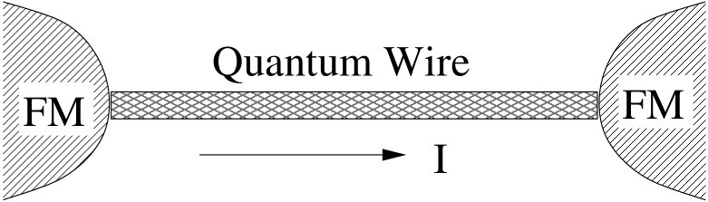
FIG. 1.: Proposed experimental setup (schematic). An individual SWNT or quantum wire is connected via low-conductance contacts to two ferromagnetic reservoirs, and $I-V$ curves should be measured either in an additional magnetic field or for various angles between the magnetization directions in the leads.

FIG. 2.: Self-energy diagram to estimate the decay time for the spin current.

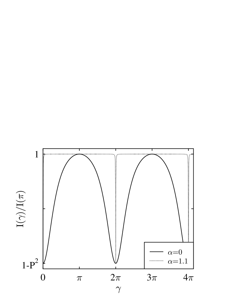
FIG. 3.: Magnetic field dependence of the $T=0$ current for $\theta=\pi$, $G=0.08e^{2}/h$, $eV/D=0.1$, $\vartheta=0.5$, both for a Fermi liquid ($\alpha=0$) and for a LL with $\alpha=1.1$, where $\vec{B}\perp\hat{m}_{1}$. The precession phase $\gamma\sim B$ is given in Eq. (90).

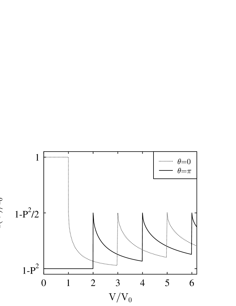
FIG. 4.: Current-voltage relation in the presence of backscattering for $T=0$ and $\theta=0,\pi$. The scales are set by $I_{0}=2I_{\alpha}$ and $V_{0}=V_{0}(\theta=0)$.

REFERENCES

- [1] A. G. Aronov, JETP Lett. 24, 32 (1976).
- [2] M. Johnson and R. H. Silsbee, Phys. Rev. Lett. 55, 1790 (1985); M. Johnson, ibid. 70, 2142 (1993).
- [3] G. A. Prinz, Physics Today 48(4), 58 (1995).
- [4] D. D. Awschalom and J. M. Kikkawa, Physics Today 52(6), 33 (1999).
- [5] M. A. M. Gijs and G. E. W. Bauer, Adv. Phys. 46, 285 (1997).
- [6] C. H. Bennett and D. P. DiVincenzo, Nature 404, 247 (2000).
- [7] A. O. Gogolin, A. A. Nersesyan, and A. M. Tsvelik, Bosonization and Strongly Correlated Systems (Cambridge University Press, 1998).
- [8] M. Bockrath, D. H. Cobden, J. Lu, A. G. Rinzler, R. E. Smalley, L. Balents, and P. L. McEuen, Nature 397, 598 (1999); Z. Yao, H. W. J. Postma, L. Balents, and C. Dekker, ibid. 402, 273 (1999).
- [9] C. Dekker, in Physics Today (May 1999). See also Special Issue on carbon nanotubes in Physics World (June 2000).
- [10] R. Egger and A. O. Gogolin, Phys. Rev. Lett. 79, 5082 (1997); Eur. Phys. J B 3, 281 (1998); C. L. Kane, L. Balents, and M. P. A. Fisher, ibid. 79, 5086 (1997).
- [11] See, e.g. K.-V. Pham, M. Gabay, and P. Lederer, Eur. Phys. J. B 9, 573 (1999).
- [12] P. W. Anderson, The Theory of Superconductivity in the High- Cuprate Superconductors (Princeton Univ. Press, Princeton, NJ, 1997).
- [13] G. Baskaran, Z. Zou, and P.W. Anderson, Solid State Comm. 63, 973 (1987); Z. Zou and P.W. Anderson, Phys. Rev. B 37, 627 (1988); N. Nagaosa and P.A. Lee, Phys. Rev. Lett. 64, 2450 (1990).
- [14] L. Balents, M. P. A. Fisher, and C. Nayak, Int. J. Mod. Phys. B 12, 1033 (1998); Phys. Rev. B 60, 1654 (1999); ibid. 61, 6307 (2000).
- [15] T. Senthil and M. P. A. Fisher, Phys. Rev. B 62, 7850 (2000).
- [16] L. Balents and R. Egger, Phys. Rev. Lett. 85, 3464 (2000).
- [17] Q. Si, Phys. Rev. Lett. 78, 1767 (1997).
- [18] Q. Si, Phys. Rev. Lett. 81, 3191 (1998).
- [19] K. Tsukagoshi, B. W. Alphenaar, and H. Ago, Nature 401, 572 (1999).
- [20] A. Brataas, Yu.V. Nazarov, and G.E.W. Bauer, Phys. Rev. Lett. 84, 2481 (2000); preprint cond-mat/0006174; D. Huertas Hernando, Yu. V. Nazarov, A. Brataas, and G. E. W. Bauer, Phys. Rev. B 62, 5700 (2000).
- [21] For a recent exposition of Stoner ferromagnetism, see P. Fazekas, Electron Correlation and Magnetism (World Scientific, Singapore, 1999).
- [22] J. Slonczewski, Phys. Rev. B 39, 6995 (1989).
- [23] J. Cardy, Scaling and Renormalization in Statistical Physics (Cambridge University Press, Cambridge, 1996).
- [24] S. Sachdev, Quantum Phase Transitions (Cambridge University Press, Cambridge, 1999).
- [25] L. D. Landau and E. M. Lifshitz, Statistical Physics, Part 2, (Pergamon Press, New York, 1980).
- [26] Away from , assuming nonzero exchange and , our results hold for arbitrary . Furthermore, for , only the weaker condition has to be imposed.
- [27] K. K. Likharev, Dynamics of Josephson Junctions and Circuits, p.65 (Gordon and Breach Science Publishers, 1986).
- [28] W. H. Press et al., Numerical Recipes (Cambridge University Press, 1992).
- [29] C. L. Kane and M. P. A. Fisher, Phys. Rev. B 46, 15 233 (1992).
- [30] L. Balents and M. P. A. Fisher, Phys. Rev. B 53, 12 133 (1996).
- [31] A. F. Andreev, Sov. Phys. JETP 19, 1228 (1964).
- [32] Single Charge Tunneling, edited by H. Grabert and M. H. Devoret, NATO-ASI Series B, Vol. 294 (Plenum Press, New York, 1992).
- [33] A. Brataas, Yu. V. Nazarov, J. Inoue, and G. E. W. Bauer, Phys. Rev. B 59, 93 (1999).
- [34] L. Balents, Proc. of the XXXIVth Rencontres de Moriond “Quantum Physics at Mesoscopic Scale”, Les Arcs, France (1999); in press; cond-mat/9906032.