Analysis of the computational complexity of solving random satisfiability problems using branch and bound search algorithms.

Abstract

The computational complexity of solving random 3-Satisfiability (3-SAT) problems is investigated. 3-SAT is a representative example of hard computational tasks; it consists in knowing whether a set of $\alpha N$ randomly drawn logical constraints involving $N$ Boolean variables can be satisfied altogether or not. Widely used solving procedures, as the Davis-Putnam-Loveland-Logeman (DPLL) algorithm, perform a systematic search for a solution, through a sequence of trials and errors represented by a search tree. The size of the search tree accounts for the computational complexity, i.e. the amount of computational efforts, required to achieve resolution. In the present study, we identify, using theory and numerical experiments, easy (size of the search tree scaling polynomially with $N$) and hard (exponential scaling) regimes as a function of the ratio $\alpha$ of constraints per variable. The complexity is explicitly calculated in the different regimes, in very good agreement with numerical simulations. Our theoretical approach is based on the analysis of the growth of the branches in the search tree under the operation of DPLL. On each branch, the initial 3-SAT problem is dynamically turned into a more generic 2+p-SAT problem, where $p$ and $1-p$ are the fractions of constraints involving three and two variables respectively. The growth of each branch is monitored by the dynamical evolution of $\alpha$ and $p$ and is represented by a trajectory in the static phase diagram of the random 2+p-SAT problem. Depending on whether or not the trajectories cross the boundary between satisfiable and unsatisfiable phases, single branches or full trees are generated by DPLL, resulting in easy or hard resolutions. Our picture for the origin of complexity can be applied to other computational problems solved by branch and bound algorithms.

PACS Numbers : 05.10, 05.70, 89.80

I Introduction.

Out-of-equilibrium dynamical properties of physical systems form the subject of intense studies in modern statistical physics[1]. Over the past decades, much progress has been made in fields as various as glassy dynamics, growth processes, persistence phenomena, vortex depinning … where dynamical aspects play a central role. Among all the questions related to these issues, the existence and characterization of stationary states reached in some asymptotic limit of large times is of central importance. In turn, the notion of asymptotic regime raises the question of relaxation, or transient, behavior: what time do we need to wait for in order to let the system relax? How does this time grow with the size of the system? Such interrogations are not limited to out-of-equilibrium dynamics but also arise in the study of critical slowing down phenomena accompanying second order phase transitions.

Computer science is another scientific discipline where dynamical issues are of central importance. There, the main question is to know the time or, more precisely, the amount of computational resources required to solve some given computational problem, and how this time increases with the size of the problem to be solved[2]. Consider for instance the sorting problem[3]. One is given a list ${\cal L}$ of $N$ integer numbers to be sorted in increasing order. What is the computational complexity of this task, that is, the minimal number of operations (essentially comparisons) necessary to sort any list ${\cal L}$ of length $N$? Knuth answered this question in the early seventies: complexity scales at least as $N\log N$ and there exists a sorting algorithm, called Mergesort, achieving this lower bound[3].

To calculate computational complexity, one has to study how the configuration of data representing the computational problem dynamically evolves under the prescriptions encoded in the algorithm. Let us consider the sorting problem again and think of the initial list ${\cal L}$ as a (random) permutation of ${\cal I}=\{1,2,\ldots,N\}$. Starting from ${\cal L}(0)={\cal L}$, at each time step (operation) $T$, the sorting algorithm transforms the list ${\cal L}(T)$ into another list ${\cal L}(T+1)$, reaching finally the identity permutation, i.e. the ordered list ${\cal I}$. Obviously, the dynamical rules imposed by a solving algorithm are of somewhat unusual nature from a physicist’s point of view. They might be highly non-local and non-Markovian. Yet, the operation of algorithms gives rise to well posed dynamical problems, to which methods and techniques of statistical physics may be applied as we argue in this paper.

Unfortunately, not all problems encountered in computer science are as simple as sorting. Many computational problems originating from industrial applications, e.g. scheduling, planning and more generally optimization tasks, demand computing efforts growing enormously with their size $N$. For such problems, called NP–complete, all known solving algorithms have execution times increasing a priori exponentially with $N$ and it is a fundamental conjecture of computer science that no polynomial solving procedure exists. To be more concrete, let us focus on the 3-satisfiability (3-SAT) problem, a paradigm of the class of NP–complete computational problems[2]. A pedagogical introduction to the 3-SAT problem and some of the current open issues in theoretical computer science may be found in [4].

3-SAT is defined as follows. Consider a set of $N$ Boolean variables and a set of $M=\alpha\,N$ constraints (called clauses), each of which being the logical OR of three variables or of their negation. Then, try to figure out whether there exists or not an assignment of variables satisfying all clauses. If such a solution exists, the set of clauses (called instance of the 3-SAT problem) is said satisfiable (sat); otherwise the instance is unsatisfiable (unsat). To solve a 3-SAT instance, i.e. to know whether it is sat or unsat, one usually resorts to search algorithms, as the ubiquitous Davis–Putnam–Loveland–Logemann (DPLL) procedure[4, 5, 6]. DPLL operates by trials and errors, the sequence of which can be graphically represented as a search tree. Computational complexity is the amount of operations performed by the solving algorithm and is conventionally measured by the size of the search tree.

Complexity may, in practice, vary enormously with the instance of the 3-SAT problem under consideration. To understand why instances are easy or hard to solve, computer scientists have focused on model classes of 3-SAT instances. Probabilistic models, that define distributions of random instances controlled by few parameters, are particularly useful. An example, that has attracted a lot of attention over the past years, is random 3-SAT: all clauses are drawn randomly and each variable negated or left unchanged with equal probabilities. Experiments[6, 7, 8, 9, 10] and theory[11, 12] indicate that instances are almost surely always sat (respectively unsat) if $\alpha$ is smaller (resp. larger) than a critical threshold $\alpha_{C}\simeq 4.3$ as soon as $M,N$ go to infinity at fixed ratio $\alpha$. This phase transition[12, 13] is accompanied by a drastic peak of computational hardness at threshold[6, 7, 8], see Figure 1. Random 3-SAT generates simplified and idealized versions of real-world instances. Yet, it reproduces essential features (sat vs. unsat, easy vs. hard) and can shed light on the onset of complexity, in the same way as models of condensed matter physics help to understand global properties of real materials.

Phases in random 3-SAT, or in physical systems, characterize the overall static behavior of a sample in the large size limit – a large instance with ratio e.g. $\alpha=3$ will be almost surely sat (existence proof) – but do not convey direct information of dynamical aspects – how long it will take to actually find a solution (constructive proof). This situation is reminiscent of the learning problem in neural networks (“equilibrium” statistical mechanics allows to compute the maximal storage capacity, irrespective of the memorization procedure and of the learning time) [14], or liquids at low enough temperatures (that should crystallize from a thermodynamical point of view but undergo some kinetical glassy arrest)[15].

This paper is an extended version of a previous work [17], where we showed how the dynamics induced by the DPLL search algorithm could be analyzed using off-equilibrium statistical mechanics and combined to the static phase diagram of random K-SAT (with K=2,3) to calculate computational complexity. We start by exposing in a detailed way the definition of the random K-SAT problem and the DPLL procedure in Section II. We then expose the experimental measures of complexity in Section III. Our analytical approach is based on the fact that, under DPLL action, the initial instance is modified and follows some trajectory in the phase diagram. The structure of the search tree generated by DPLL procedure is closely related to the nature of the region visited by the instance trajectory. Search trees reduce to essentially one branch – sat instances at low ratio $\alpha$, section IV – or are dense, including an exponential number of branches – unsat instances, section V. Mixed structures – sat instances with ratios slightly below threshold, section VI – are made of a branch followed by a dense tree and reflect trajectories crossing the phase boundary between sat and unsat regimes. While branch trajectories could be obtained straightforwardly from previous works by Chao and Franco[18], we develop in section V a formalism to study the construction of dense trees by DPLL. We show that the latter can be reformulated in terms of a (bidimensional) growth process described by a non-linear partial differential equation. The resolution of this growth equation allows an analytical prediction of the complexity that compares very well to extensive numerical experiments. We present in Section VII the full complexity diagram of solving random SAT models, and explain the relationship with static studies of the phase transition [13]. Last of all, we show in Section VIII how our study suggests some possible ways to improve existing algorithms.

II Davis-Putnam-Loveland-Logeman algorithm and random 3-SAT.

In this section, the reader will be briefly recalled the main features of the random 3-Satisfiability model. We then present the Davis-Putnam-Loveland-Logeman (DPLL) solving procedure, a paradigm of branch and bound algorithm, and the notion of search tree. Finally, we introduce the idea of dynamical trajectory, followed by an instance under the action of DPLL.

A A reminder on random Satisfiability.

Random K-SAT is defined as follows. Let us consider $N$ Boolean variables $x_{i}$ that can be either true (T) or false (F) ($i=1,\ldots,N)$. We choose randomly $K$ among the $N$ possible indices $i$ and then, for each of them, a literal, that is, the corresponding $x_{i}$ or its negation $\bar{x}_{i}$ with equal probabilities one half. A clause $C$ is the logical OR of the $K$ previously chosen literals, that is $C$ will be true (or satisfied) if and only if at least one literal is true. Next, we repeat this process to obtain $M$ independently chosen clauses $\{C_{\ell}\}_{\ell=1,\ldots,M}$ and ask for all of them to be true at the same time (i.e. we take the logical AND of the $M$ clauses). The resulting logical formula is called an instance of the K-SAT problem. A logical assignment of the $x_{i}$’s satisfying all clauses, if any, is called a solution of the instance.

For large instances ($M,N\to\infty$), K-SAT exhibits a striking threshold phenomenon as a function of the ratio $\alpha=M/N$ of the number of clauses per variable. Numerical simulations indicate that the probability of finding a solution falls abruptly from one down to zero when $\alpha$ crosses a critical value $\alpha_{C}(K)$[6, 7, 8]. Above $\alpha_{C}(K)$, all clauses cannot be satisfied any longer. This scenario is rigorously established in the $K=2$ case, where $\alpha_{C}=1$[19]. For $K\geq 3$, much less is known; $K(\geq 3)$–SAT belongs to the class of hard, NP-complete computational problems[2]. Studies have mainly concentrated on the $K=3$ case, whose instances are simpler to generate than for larger values of $K$. Some lower [20] and upper [21] bounds on $\alpha_{C}(3)$ have been derived, and numerical simulations have recently allowed to find precise estimates of $\alpha_{C}$, e.g. $\alpha_{C}(3)\simeq 4.3$[8, 10].

The phase transition taking place in random 3-SAT has attracted a large deal of interest over the past years due to its close relationship with the emergence of computational complexity. Roughly speaking, instances are much harder to solve at threshold than far from criticality [6, 7, 8, 9]. We now expose the solving procedure used to tackle the 3-SAT problem.

B The Davis-Putnam-Loveland-Logeman solving procedure.

1 Main operations of the solving procedure and search trees.

3-SAT is among the most difficult problems to solve as its size $N$ becomes large. In practice, one resorts to methods that need, a priori, exponentially large computational resources. One of these algorithms, the Davis–Putnam–Loveland–Logemann (DPLL) solving procedure[4, 5], is illustrated on Figure 1. DPLL operates by trials and errors, the sequence of which can be graphically represented as a search tree made of nodes connected through edges as follows:

• A node corresponds to the choice of a variable. Depending on the value of the latter, DPLL takes one of the two possible edges.

• Along an edge, all logical implications of the last choice made are extracted.

• DPLL goes back to step 1 unless a solution is found or a contradiction arises; in the latter case, DPLL backtracks to the closest incomplete node (with a single descendent edge), inverts the attached variable and goes to step 2; if all nodes carry two descendent edges, unsatisfiability is proven.

Examples of search trees for satisfiable (sat) or unsatisfiable (unsat) instances are shown Figure 2. Computational complexity is the amount of operations performed by DPLL, and is measured by the size of the search tree, i.e. the number of nodes.

2 Heuristics of choice.

In the above procedure, step 1 requires to choose one literal among the variables not assigned yet. The choice of the variable and of its value obeys some more or less empirical rules called splitting heuristics. The key idea is to choose variables that will lead to the maximum number of logical implications [22]. Here are some simple heuristics:

• “Truth table” rule: fix unknown variables in lexicographic order, from $x_{1}$ up to $x_{N}$ and assign them to e.g. true. This is an inefficient rule that does not follow the key principle exposed above.

• Generalized Unit-Clause (GUC) rule: choose randomly one literal among the shortest clauses[18]. This is an extension of unit-propagation that fixes literal in unitary clauses. GUC is based on the fact that a clause of length $K$ needs at most $K-1$ splittings to produce a logical implication. So variables are chosen preferentially among short clauses.

• Maximal occurrence in minimum size clauses (MOMS) rule: pick up the literal appearing most often in shortest clauses. This rule is a refinement of GUC.

Global performances of DPLL depend quantitatively on the splitting rule. From a qualitative point of view, however, the easy-hard-easy picture emerging from experiments is very robust [7, 8, 10]. Hardest instances seem to be located at threshold. Solving them demand an exponentially large computational effort scaling as $2^{N\omega_{C}}$. The values of $\omega_{C}$ found in literature roughly range from $0.05$ to $0.1$, depending on the splitting rule used by DPLL[6, 22].

In this paper, we shall focus on the GUC heuristic which is simple enough to allow analytical studies and, yet, is already quite efficient.

C 2+p-SAT and instance trajectory.

We shall present in Section III the experimental results on solving 3-SAT instances using DPLL procedure in a detailed way. The main scope of this paper is to compute in an analytical way the computational complexity $\omega$ in the easy and hard regimes. To do so, we have made use of the precious notion of dynamical trajectory, that we now expose.

As shown in Figure 3, the action of DPLL on an instance of 3-SAT causes the reduction of 3-clauses to 2-clauses. Thus, a mixed 2+p-SAT distribution[13], where $p$ is the fraction of 3-clauses, may be used to model what remains of the input instance at a node of the search tree. A 2+p-SAT formula of parameters $p,\alpha$ is the logical AND of two uncorrelated random 2-SAT and 3-SAT instances including $\alpha\,(1-p)\,N$ and $\alpha\,p\,N$ clauses respectively. Using experiments[13] and statistical mechanics calculations[12], the threshold line $\alpha_{C}(p)$ may be obtained with the results shown in Figure 4 (full line). Replica calculations suggest that the sat/unsat transition taking place at $\alpha_{C}(p)$ is continuous if $p<p_{S}$ and discontinuous if $p>p_{S}$, where $p_{S}\simeq 0.41$[23]. The tricritical point T_S is shown in Figure 4. Below $p_{s}$, the threshold $\alpha_{C}(p)$ coincides with the upper bound $1/(1-p)$, obtained when requiring that the 2-SAT subformula only be satisfied. Rigorous studies have shown that $p_{S}\geq 2/5$, leaving open the possibility it is actually equal to 2/5[24], or to some slightly larger value[25].

The phase diagram of 2+p-SAT is the natural space in which DPLL dynamic takes place[17]. An input 3-SAT instance with ratio $\alpha_{0}$ shows up on the right vertical boundary of Figure 4 as a point of coordinates $(p=1,\alpha_{0})$. Under the action of DPLL, the representative point moves aside from the 3-SAT axis and follows a trajectory. The location of this trajectory in the phase diagram allows a precise understanding of the search tree structure and of complexity.

III Numerical Experiments.

A Description of the numerical implementation of the DPLL algorithm.

We have implemented DPLL with the GUC rule, see Figure 3 and Section II B 2, to have a fast unit propagation and an inexpensive backtracking [6]. The program is divided in three parts. The first routine draws the clauses and represents the data in a convenient structure. The second, main routine updates and saves the state of the search, i.e. the indices and values of assigned variables, to allow an easy backtracking. Then, it checks if a solution is found; if not, a new variable is assigned. The third routine extracts the implication of the choice (propagation). If unit clauses have been generated, the corresponding literals are fixed, or a contradiction is detected.

1 Data Representation

Three arrays are used to encode the data: the two first arrays are labelled by the clause number $m=1,\ldots,M$ and the number $b=1,\ldots,K$ of the components in the clause (with $K=2,3$). The entries of these arrays, initially drawn at random, are the indices $clausnum\,(m,b)$ and the values $clausval\,(m,b)$, true or false, of the variables. The indices of the third array are integers $i=1,\ldots,N$ and $j=1,\ldots,o_{i}$ where $o_{i}$ is the number of occurrences of $x_{i}$ in the clauses (from zero to $M$). The entries of the matrix, $a\,(i,j)$, are the numbers of the corresponding clauses (between 1 and $M$).

2 Updating of the search state.

If the third routine has found a contradiction, the second routine goes back along the branch, inverts the last assigned variable and calls again the third routine. If not, the descent along the branch is pursued. A Boolean-valued vector points to the assigned variables, while the values are stored in another unidimensional array. For each clause, we check if the variables are already assigned and, if so, if they are in agreement or not with the clauses. When splitting occurs, a new variable is fixed to satisfy a 2-clause, i.e. a clause with one false literal and two unknown variables, and the third subroutine is called. If there are only 3-clauses, a new variable is fixed to satisfy any 3-clause and the third subroutine is called. The variable chosen and its value are stored in a vector with index the length of the branch, i.e. the number of nodes it contains, to allow future backtracking. If there are neither 2- nor 3-clauses left, a solution is found.

3 Consequences of a choice and unit propagation

All clauses containing the last fixed variable are analyzed by taking into account all possibilities: 1. the clause is satisfied; 2. the clause is reduced to a 2- or 1-clause; 3. the clause is violated (contradiction). In the second case, the 1-clause is stored to be analyzed by unit-propagation once all clauses containing the variable have been reviewed.

B Characteristic running times

We have implemented the DPLL search algorithm in Fortran 77; the algorithm runs on a Pentium II PC with a 433M Hz frequency clock. The number of nodes added per minute ranges from 300,000 (typically obtained for $\alpha=3.5$) to 100,000 ($\alpha=10$) since unit propagation is more and more frequent as $\alpha$ increases. The order of magnitude of the computational time needed to solve an instance are listed in Table I for ratios corresponding to hard instances. These times limit the maximal size $N$ of the instances we have experimentally studied and the number of samples over which we have averaged. Some rare instances may be much harder than the typical times indicated in Table I. For instance, for $\alpha=3.1$ and $N=500$, instances are usually solved in about 4 minutes but some samples required more than 2 hours of computation. Such a phenomenon will be discussed in Section III D 1.

C Overview of experiments

1 Number of nodes of the search tree

We have first investigated complexity by a direct count of the number of splittings, that is the number of nodes (black points) in Figure 2, for sat (Figure 2A,C) and unsat (Figure 2B) trees.

2 Histogram of branch length.

We have also experimentally investigated the structure of search trees for unsat instances (Figure 2B). A branch is defined as a path joining the root (first node on the top of the search tree) to a leaf marked with a contradiction $C$ (or a solution $S$ for sat instance) in Figure 2. The length of a branch is the number of nodes it contains. For an unsat instance, the complete search tree depends on the variables chosen at each split, but not on the values they are assigned to. Indeed, to prove that there is no solution, all nodes in the search tree have to carry two outgoing branches, corresponding to the two choices of the attached variables. What choice is made first does not matter. This simple remark will be of crucial importance in the theoretical analysis of Section V B 1.

We have derived the histogram of the branch lengths by counting the number $B(l)$ of branches having length $l\,N$ once the tree is entirely built up. The histogram is very useful to deduce the complexity in the unsat phase, since in a complete tree the total number of branches $B$ is related to the number of nodes $Q$ through the identity,

$$B=\sum_{l=\frac{1}{N},\ldots,1}B(l)=Q+1\qquad.$$ (1)

that can be inferred from Figure 2B.

3 Highest backtracking point

Another key property we have focused upon is the highest backtracking point in the search tree. In the unsat phase, DPLL backtracks all the nodes of the tree since no solution can be present. The highest backtracking point in the tree simply coincides with the top (root) node. In the sat phase, the situation is more involved. A solution generally requires some backtracking and the highest backtracking node may be defined as the closest node to the origin through which two branches pass, node $G$ on Figure 2B. We experimentally keep trace of the highest backtracking point by measuring the numbers $C_{2}(G)$, $C_{3}(G)$ of 2- and 3-clauses, the number of not-yet-assigned variables $N(G)$, and computing the coordinates $p_{G}=C_{3}(G)/(C_{2}(G)+C_{3}(G)),\alpha_{G}=(C_{2}(G)+C_{3}(G))/N(G)$ of $G$ in the phase diagram of Figure 4.

D Experimental Results

1 Fluctuations of complexity.

The size of the search tree built by DPLL is a random variable, due to the (quenched) randomness of the 3-SAT instance and the choices made by the splitting rule (“thermal noise”). We show on Figure 5 the distribution of the logarithms (in base 2, and divided by $N$) of the number of nodes for different values of $N$. The distributions are more and more peaked around their mean values $\omega_{N}(\alpha)$ as the size $N$ increases. This indicates that the logarithm of the complexity is a self-averaging quantity in the thermodynamic limit. However, fluctuations are dramatically different at low and large ratios. For $\alpha=10$, and more generally in the unsat phase, the distributions are roughly symmetric (Figure 5A). Tails are small and complexity does not fluctuate too much from sample to sample[26, 27]. In the vicinity of $\alpha_{L}$, e.g. $\alpha=3.1$, much bigger fluctuations are present. There are large tails on the right flanks of the distributions on Figure 5B, due to the presence of rare and very hard samples [27]. Complexity is not self-averaging. We will come back to this point in section VI.

2 The easy-hard-easy pattern.

We have averaged the logarithm of the number of nodes over 10,000 randomly drawn instances to obtain $\omega_{N}(\alpha)$. The typical size $Q$ of the search tree is simply $Q=2^{N\omega_{N}}$. Results are shown in Figure 1. An easy-hard-easy pattern of complexity appears clearly as the ratio $\alpha$ varies.

• At small ratios, complexity increases as $\gamma(\alpha)N$, that is, only linearly with the size of the instance. DPLL easily finds a solution and the search tree essentially reduces to a single branch shown on Figure 2A. For the GUC heuristic, the linear regime extends up to $\alpha_{L}\simeq 3.003$ [18, 20].

• Above threshold, complexity grows exponentially with $N$[28]. The logarithm $\omega(\alpha)$, limit of $\omega_{N}(\alpha)$ as $N\to\infty$, is maximal at criticality…

• … and decreases at large ratios as $1/\alpha$ [29]. The “easy” region on the right hand side of Figure 1 is still exponential but with small coefficients $\omega$.

Of particular interest is the intermediate region $\alpha_{L}<\alpha<\alpha_{C}$. We shall show that complexity is exponential in this range of ratios, and that the search tree is a mixture of the search trees taking place in the other ranges $\alpha<\alpha_{L}$ and $\alpha>\alpha_{C}$.

Let us mention that, while this paper is devoted to typical-case (happening with probability one) complexity, rigorous results have been obtained that apply to any instance. So far, using a refined version of DPLL, any instance is guaranteed to be solved in less than $1.504^{N}$ steps, i.e. $\omega<0.588$. The reader is referred to reference [30] for this worst-case analysis.

3 Lower sat phase ($\alpha<\alpha_{L}$)

The complexity data of Figure 1 obtained for different sizes $N=50,75,100$ are plotted again on Figure 6 after division by $N$. Data collapse on a single curve, proving that complexity is linear in the regime $\alpha<\alpha_{L}$. In the vicinity of the cross over ratio $\alpha=\alpha_{L}$ finite-size effects became important in this region. We have thus performed extra simulations for larger sizes $N=500,1000$ in the range $2.5\leq\alpha\leq 3.$ that confirm the linear scaling of the complexity.

4 Unsat Phase ($\alpha>\alpha_{C}$)

Results for the shape of the search trees are shown in Figure 7. We represent the logarithm $b(l)$, in base 2 and divided by $N$, of the number $B(l)$ of branches as a function of the branch length $l$, averaged over many samples and for different sizes $N$ and ratios $\alpha.$ When $\alpha$ increases at fixed $N$, branches are shorter and shorter and less and less numerous, making complexity decrease (Figure 1).

As $N$ gets large at fixed $\alpha$, the histogram $b(l)$ becomes a smooth function of $l$ and we can replace the discrete sum in (1) with a continuous integral on the length,

$$Q+1=\sum_{l=\frac{1}{N},\ldots,1}2^{N\,b(l)}\simeq N\int_{0}^{1}dl\;2^{N\,b(l)}\qquad.$$ (2)

The integral is exponentially dominated by the maximal value $b_{max}$ of $b(l)$. $\omega$, the limit of the logarithm of the complexity divided by $N$, is therefore equal to $b_{max}$. Nicely indeed, the height $b_{max}$ of the histogram does not depend on $N$ (within the statistical errors) and gives a straightforward and precise estimate of $\omega$, not affected by finite-size effects. The values of $b_{max}$ as a function of $\alpha$ are listed in the third column of Table II.

The above discussion is also very useful to interpret the data on the size $Q$ of the search trees. From the quadratic correction around the saddle-point, $b(l)\simeq b_{max}-\beta(l-l_{max})^{2}/2$, the expected finite size correction to $\omega_{N}$ read

$$\omega_{N}\simeq\omega+\frac{1}{2N}\log_{2}N+\frac{1}{2N}\log_{2}\left[\frac{2\pi}{\beta\ln 2}\right]+O\left(\frac{1}{N^{2}}\right)\qquad.$$ (3)

We have checked the validity of this equation by fitting $\omega_{N}-\log_{2}N/(2N)$ as a polynomial function of $1/N$. The constant at the origin gives values of $\omega$ in very good agreement with $b_{max}$ (second column in Table II) while the linear term gives access to the curvature $\beta$. We compare in Table III this curvature with the direct measurements of $\beta$ obtained by looking at the vicinity of the top of the histogram. The agreement is fair, proving that equation (3) is an accurate way of extrapolating data on $Q$ to the infinite size limit.

5 Upper sat phase ($\alpha_{L}<\alpha<\alpha_{C}$)

To investigate the sat region slightly below threshold $\alpha_{L}<\alpha<\alpha_{C}$, we have carried out simulations with a starting ratio $\alpha=3.5$. Results are shown on Figure 8A. As instances are sat with a high probability, no simple identity relates the number of nodes $Q$ to the number of branches $B$, see search tree in Figure 2C and we measure the complexity through $Q$ only. Complexity clearly scales exponentially with the size of the instance and exhibits large fluctuations from sample to sample. The annealed complexity (logarithm of the average complexity), $\omega_{3}^{ann}$, is larger than the typical solving hardness (average of the logarithm of the complexity), $\omega_{3}^{typ}$, see Table IV.

To reach a better understanding of the structure of the search tree, we have focused on the highest backtracking point G defined in Figure 2C and Section III C 3. The coordinates $p_{G},\alpha_{G}$ of point G, averaged over instances are shown for increasing sizes $N$ on Figure 9. The coordinates of G exhibit strong sample fluctuations which make the large $N$ extrapolation, $p_{G}=0.78\pm 0.01$, $\alpha_{G}=3.02\pm 0.02$ rather imprecise.

In Section VI, we shall show how the solving complexity in the upper sat phase is related to the solving complexity of corresponding 2+p-SAT problems with parameters $p_{G},\alpha_{G}$.

IV Branch Trajectories and the linear regime (lower sat phase).

In this section, we investigate the dynamics of DPLL in the low ratio regime, where a solution is rapidly found (in a linear time) and the search tree essentially reduces to a single branch shown Figure 2. We start with some general comments on the dynamics induced by DPLL (section IV A), useful to understand how the trajectory followed by the instance can be computed in the $p,\alpha$ plane (section IV B). These two first sections merely expose some previous works by Chao and Franco, and the reader is asked to consult [18] for more details. In the last section IV C, our numerical and analytical results for the solving complexity are presented.

In this Section, as well as in Sections V and VI, the ratio of the 3-SAT instance to be solved will be denoted by $\alpha_{0}$.

A Remarks on the dynamics of clauses.

1 Dynamical flows of populations of clauses.

As pointed out in Section II C, under the action of DPLL, some clauses are eliminated while other ones are reduced. Let us call $C_{j}(T)$ the number of clauses of length $j$ (including $j$ variables), once $T$ variables have been assigned by the solving procedure. $T$ will be called hereafter “time”, not to be confused with the computational time necessary to solve a given instance. At time $T=0$, we obviously have $C_{3}(0)=\alpha_{0}N$, $C_{2}(0)=C_{1}(0)=0$. As some Boolean variables are assigned, the time $T$ increases and clauses of length one or two are produced. A sketchy picture of DPLL dynamics at some instant $T$ is proposed in Figure 10.

We call $e_{1},e_{2},e_{3}$ and $w_{2},w_{1}$ the flows of clauses represented in Figure 10 when times increases from $T$ to $T+1$, that is, when one more variable is chosen by DPLL after $T$ have already been assigned. The evolution equations for the three populations of clauses read,

$$C_{3}(T+1) = C_{3}(T)-e_{3}(T)-w_{2}(T)$$ (4)

$$C_{2}(T+1) = C_{2}(T)-e_{2}(T)+w_{2}(T)-w_{1}(T)$$ (5)

$$C_{1}(T+1) = C_{1}(T)-e_{1}(T)+w_{1}(T)\qquad.$$ (6)

The flows $e_{j}$ and $w_{j}$ are of course random variables that depend on the instance under consideration at time $T$, and on the choice of the variable (label and value) done by DPLL. For a single descent, i.e. in the absence of backtracking, the evolution process (6) is Markovian and unbiased. The distribution of instances generated by DPLL at time $T$ is uniform over the set of all the instances having $C_{j}(T)$ clauses of length $j=1,2,3$ and drawn from a set of $N-T$ variables[18].

2 Concentration of distributions of populations.

As a result of the additivity of (6), some concentration phenomenon takes place in the large size limit. The numbers of clauses of lengths 2 and 3, a priori extensive in $N$, do not fluctuate too much,

$$C_{j}(T)=N\;c_{j}\left(\frac{T}{N}\right)+o(N)\qquad(j=2,3)\ .$$ (7)

where the $c_{j}$’s are the densities of clauses of length $j$ averaged over the instance (quenched disorder) and the choices of variables (“thermal” disorder). In other words, the populations of 2- and 3-clauses are self-averaging quantities and we shall attempt at calculating their mean densities only. Note that, in order to prevent the occurrence of contradictions, the number of unitary clauses must remain small and the density $c_{1}$ of 1-clauses has to vanish.

3 Time scales separation and deterministic vs. stochastic evolutions.

Formula (7) also illustrates another essential feature of the dynamics of clause populations. Two time scales are at play. The short time scale, of the order of the unity, corresponds to the fast variations of the numbers of clauses $C_{j}(T)$ ($j=1,2,3$). When time increases from $T$ to $T+O(1)$ (with respect to the size $N$), all $C_{j}$’s vary by $O(1)$ amounts. Consequently, the densities of clauses $c_{j}$, that is, their numbers divide by $N$, are not modified. The densities $c_{j}$s evolve on a long time scale of the order of $N$ and depend on the reduced time $t=T/N$ only.

Due to the concentration phenomenon underlined above, the densities $c_{j}(t)$ will evolve deterministically with the reduced time $t$. We shall see below how Chao and Franco calculated their values. On the short time scale, the relative numbers of clauses $D_{j}(T)=C_{j}(T)-Nc_{j}(T/N)$ fluctuate (with amplitude $\ll N$) and are stochastic variables. As said above the evolution process for these relative numbers of clauses is Markovian and the probability rates (master equation) are functions of slow variables only, i.e. of the reduced time $t$ and of the densities $c_{2}$ and $c_{3}$ only. As a consequence, on intermediary time scales, much larger than unity and much smaller than $N$, the $D_{j}$s may reach some stationary distribution that depend upon the slow variables.

This situation is best exemplified in the case $j=1$ where $c_{1}(t)=0$ as long as no contradiction occurs and $D_{1}(T)=C_{1}(T)$. Consider for instance a time delay $1\ll\Delta T\ll N$, e.g. $\Delta T=\sqrt{N}$. For times $T$ lying in between $T_{0}=t\,N$ and $T_{1}=T_{0}+\Delta T=t\,N+\sqrt{N}$, the numbers of 2- and 3-clauses fluctuate but their densities are left unchanged and equal to $c_{2}(t)$ and $c_{3}(t)$. The average number of 1-clauses fluctuates and follows some master equation whose transition rates (from $C_{1}^{\prime}=C_{1}(T)$ to $C_{1}=C_{1}(T+1)$) define a matrix ${\cal M}(C_{1},C^{\prime}_{1})$ and depend on $t,c_{2},c_{3}$ only. ${\cal M}$ has generally a single eigenvector $\mu(C_{1})$ with eigenvalue unity, called equilibrium distribution, and other eigenvectors with smaller eigenvalues (in modulus). Therefore, at time $T_{1}$, $C_{1}$ has forgotten the “initial condition” $C_{1}(T_{0})$ and is distributed according to the equilibrium distribution $\mu(C_{1})$ of the master equation.

To sum up, the dynamical evolution of the clause populations may be seen as a slow and deterministic evolution of the clause densities to which are superimposed fast, small fluctuations. The equilibrium distribution of the latter adiabatically follows the slow trajectory.

B Mathematical analysis.

In this section, we expose Chao and Franco’s calculation of the densities of 2- and 3-clauses.

1 Differential equations for the densities of clauses.

Consider first the evolution equation (6) for the number of 3-clauses. This can be rewritten in terms of the average density $c_{3}$ of 3-clauses and of the reduced time $t$,

$$\frac{dc_{3}(t)}{dt}=-z_{3}(t)\quad,$$ (8)

where $z_{3}=\langle e_{3}+w_{2}\rangle$ denotes the averaged total outflow of 3-clauses (Section IV A 2).

At some time step $T\to T+1$, 3-clauses are eliminated or reduced if and only if they contain the variable chosen by DPLL. Let us first suppose that the variable is chosen in some 1- or 2-clauses. A 3-clause will include this variable or its negation with probability $3/(N-T)$ and disappear with the same probability. Due to the uncorrelation of clauses, we obtain $z_{3}(t)=3c_{3}(t)/(1-t)$. If the literal assigned by DPLL is chosen among some 3-clause, this result has to be increased by one (since this clause will necessarily be eliminated) in the large $N$ limit.

Let us call $\rho_{j}(t)$ the probability that a literal is chosen by DPLL in a clause of length $j$ (=1,2,3). The normalization of probability imposes that

$$\rho_{1}(t)+\rho_{2}(t)+\rho_{3}(t)=1\qquad,$$ (9)

at any time $t$. Extending the above discussion to 2-clauses, we obtain

$$\frac{dc_{3}(t)}{dt} = -\frac{3}{1-t}c_{3}(t)-\rho_{3}(t)$$ (10)

$$\frac{dc_{2}(t)}{dt} = \frac{3}{2(1-t)}c_{3}(t)-\frac{2}{1-t}c_{2}(t)-\rho_{2}(t)\quad,$$ (11)

In order to solve the above set of coupled differential equations, we need to know the probabilities $\rho_{j}$. As we shall see, the values of the $\rho_{j}$ can directly be deduced from the heuristic of choice, the so-called generalized unit-clause (GUC) rule exposed in section II B 2.

The solutions of the differential equations (11) will be expressed in terms of the fraction $p$ of 3-clauses and the ratio $\alpha$ of clauses per variable using the identities

$$p(t)=\frac{c_{3}(t)}{c_{2}(t)+c_{3}(t)}\quad,\qquad\alpha(t)=\frac{c_{2}(t)+c_{3}(t)}{1-t}\quad.$$ (12)

2 Solution for $\alpha_{0}\leq 2/3$.

When DPLL is launched, 2-clauses are created with an initial flow $\langle w_{2}(0)\rangle=3\,\alpha_{0}/2$. Let us suppose that $\alpha_{0}\leq 2/3$, i.e. $w_{2}(0)\leq 1$. In other words, less than one 2-clause is created each time a variable is assigned. Since the GUC rule compels DPLL to look for literals in the smallest available clauses, 2-clauses are immediately removed just after creation and do not accumulate in their recipient. Unitary clauses are almost absent and we have

$$\rho_{1}(t)=0\ ;\quad\rho_{2}(t)=\frac{3c_{3}(t)}{2(1-t)}\ ;\quad\rho_{3}(t)=1-\rho_{2}(t)\qquad(\alpha_{0}<2/3)\ .$$ (13)

The solutions of (11) with the initial condition $p(0)=1,\alpha(0)=\alpha_{0}$ read

$$p(t) = 1\ ,$$ (14)

$$\alpha(t) = (\alpha_{0}+2)(1-t)^{3/2}-2(1-t)\quad.$$ (15)

Solution (15) confirms that the instance never contains an extensive number of 2-clauses. At some final time $t_{end}$, depending on the initial ratio, $\alpha(t_{end})$ vanishes: no clause is left and a solution is found.

3 Solution for $2/3<\alpha_{0}<\alpha_{L}$.

We now assume that $\alpha_{0}>2/3$, i.e. $\langle w_{2}(0)\rangle>1$. In other words, more than one 2-clause is created each time a variable is assigned. 2-clauses now accumulate, and give rise to unitary clauses. Due to the GUC prescription, in presence of 1- or 2-clauses, a literal is never chosen in a 3-clause. Thus,

$$\rho_{1}(t)=\frac{c_{2}(t)}{1-t}\ ;\quad\rho_{2}(t)=1-\rho_{1}(t)\ ;\quad\rho_{3}(t)=0\qquad(\alpha_{0}>2/3)\ ,$$ (16)

as soon as $t>0$. The solutions of (11) now read

$$p(t) = \frac{4\alpha_{0}(1-t)^{2}}{\alpha_{0}(1-t)^{2}+3\alpha_{0}+4\ln(1-t)}\ ,$$ (17)

$$\alpha(t) = \frac{\alpha_{0}}{4}(1-t)^{2}+\frac{3\alpha_{0}}{4}+\ln(1-t)\quad.$$ (18)

Solution (18) requires that the instance contains an extensive number of 2-clauses. This is true at small times since $p^{\prime}(0)=1/\alpha_{0}-3/2<0$. At some time $t^{*}>0$, depending on the initial ratio, $p(t^{*})$ reaches back unity: no 2-clause are left and hypothesis (16) breaks down. DPLL has therefore reduced the initial formula to a smaller 3-SAT instance with a ratio $\alpha^{*}=\alpha(t^{*})$. It can be shown that $\alpha^{*}<2/3$. Thus, as the dynamical process is Markovian, the further evolution of the instance can be calculated from Section IV B 2.

4 Trajectories in the $p,\alpha$ plane.

We show in Figure 4 the trajectories obtained for initial ratios $\alpha_{0}=0.6$, $\alpha_{0}=2$ and $\alpha_{0}=2.8$. When $\alpha_{0}>2/3$, the trajectory first heads to the left (Section IV B 3) and then reverses to the right until reaching a point on the 3-SAT axis at small ratio $\alpha^{*}(<2/3)$ without ever leaving the sat region. Further action of DPLL leads to a rapid elimination of the remaining clauses and the trajectory ends up at the right lower corner S, where a solution is achieved (section IV B 2).

As $\alpha_{0}$ increases up to $\alpha_{L}$, the trajectory gets closer and closer to the threshold line $\alpha_{C}(p)$. Finally, at $\alpha_{L}\simeq 3.003$, the trajectory touches the threshold curve tangentially at point T with coordinates $(p_{T}=2/5,\alpha_{T}=5/3)$. Note the identity $\alpha_{T}=1/(1-p_{T})$.

C Complexity.

In this section, we compute the computational complexity in the range $0\leq\alpha_{0}\leq\alpha_{L}$ from the previous results.

1 Absence of backtracking.

The trajectories obtained in section IV B 4 represent the deterministic evolution of the densities of 2- and 3-clauses when more and more variables are assigned. Equilibrium fluctuations of number of 1-clauses have been computed by Frieze and Suen [20]. The stationary distribution $\mu_{t}(C_{1})$ of the population of 1-clauses can be exactly computed at any time $t$. The most important result is the probability that $C_{1}$ vanishes,

$$\mu_{t}(0)=1-\alpha(t)\big{(}1-p(t)\big{)}\qquad.$$ (19)

$\mu_{t}(0)$ (respectively $1-\mu_{t}(0)$) may be interpreted as the probability that a variable assigned by DPLL at time $t$ is chosen through splitting (resp. unit–propagation). When DPLL starts solving a 3-SAT instance, $\mu_{t=0}(0)=1$ and many splits are necessary. If the initial ratio $\alpha_{0}$ is smaller than 2/3, this statement remains true till the final time $t_{end}$ and the absence of 1-clauses prevents the onset of contradiction. Conversely, if $2/3<\alpha_{0}<\alpha_{L}$, as $t$ grows, $\mu_{t}(0)$ decreases are more and more variables are fixed through unit-propagation. The population of 1-clauses remains finite and the probability that a contradiction occurs when a new variable is assigned is $O(1/N)$ only. However small is this probability, $O(N)$ variables are fixed along a complete trajectory. The resulting probability that a contradiction never occurs is strictly smaller than unity[20],

$${\cal P}_{No\ Contradiction}=\exp\left(-\frac{1}{4}\int_{0}^{t_{end}}\frac{dt}{1-t}\frac{(1-\mu_{t}(0))^{2}}{\mu_{t}(0)}\right)\qquad.$$ (20)

Frieze and Suen have shown that contradictions have no dramatic consequences. The number of backtrackings necessary to find a solution is bounded from above by a power of $\log N$. The final trajectory in the $p,\alpha$ plane is identical to the one shown in section IV B 4 and the increase of complexity is negligible with respect to $O(N)$.

When $\alpha_{0}$ reaches $\alpha_{L}$, the trajectory intersects the $\alpha=1/(1-p)$ line in T. At this point, $\mu(0)$ vanishes and backtracking enters massively into play, signaling the cross-over to exponential regime.

2 Length of trajectories.

From the above discussion, it appears that a solution is found by DPLL essentially at the end of a single descent (Figure 2A). Complexity thus scales linearly with $N$ with a proportionality coefficient $\gamma(\alpha_{0})$ smaller than unity.

For $\alpha_{0}<2/3$, clauses of length unity are never created by DPLL (Section IV B 2). Thus, DPLL assigns the overwhelming majority of variables by splittings. $\gamma(\alpha_{0})$ simply equals the total fraction $t_{end}$ of variables chosen by DPLL. From (15), we obtain

$$\gamma(\alpha_{0})=1-\frac{4}{(\alpha_{0}+2)^{2}}\qquad(\alpha_{0}\leq 2/3)\ .$$ (21)

For larger ratios, i.e. $\alpha_{0}>2/3$, the trajectory must be decomposed into two successive portions (Section IV B 3). During the first portion, for times $0<t<t^{*}$, 2-clauses are present with a non vanishing density $c_{2}(t)$. Some of these 2-clauses are reduced to 1-clauses that have to be eliminated next. Consequently, when DPLL assigns an infinitesimal fraction $dt$ of variables, a fraction $\rho_{1}(t)=\alpha(t)(1-p(t))dt$ are fixed by unit-propagation only. The number of nodes (divided by $N$) along the first part of the branch thus reads,

$$\gamma_{1}=t^{*}-\int_{0}^{t^{*}}dt\;\alpha(t)(1-p(t))\quad.$$ (22)

At time $t^{*}$, the trajectory touches back the 3-SAT axis $p=1$ at ratio $\alpha^{*}\equiv\alpha(t^{*})<2/3$. The initial instance is then reduces to a smaller and smaller 3-SAT formula, with a ratio $\alpha(t)$ vanishing at $t_{end}$. According to the above discussion, the length of this second part of the trajectory equals

$$\gamma_{2}=t_{end}-t^{*}\quad.$$ (23)

It results convenient to plot the total complexity $\gamma=\gamma_{1}+\gamma_{2}$ in a parametric way. To do so, we express the initial ratio $\alpha_{0}$ and the complexity $\gamma$ in terms of the end time $t^{*}$ of the first part of the branch. A simple calculation from equations (18) leads to

$$\alpha_{0}(t^{*}) = -\frac{4\ln(1-t^{*})}{3t^{*}(2-t^{*})}$$ (24)

$$\gamma(t^{*}) = 1-\frac{4(1-t^{*})}{(2+(1-t^{*})^{2}\alpha_{0}(t^{*}))^{2}}+t^{*}+(1-t^{*})\ln(1-t^{*})-\frac{1}{4}\alpha_{0}(t^{*})\;(t^{*})^{2}(3-t^{*})$$ (25)

As $t^{*}$ grows from zero to $t^{*}_{L}\simeq 0.892$, the initial ratio $\alpha_{0}$ spans the range $[2/3;\alpha_{L}]$. The complexity coefficient $\gamma(\alpha_{0})$ can be computed from equations (21,25) with the results shown Figure 6. The agreement with the numerical data of Section III D 3 is excellent.

V Tree trajectories and the exponential regime (unsat phase).

To present our analytical study of the exponentially large search trees generated when solving hard instances, we consider first a simplified growth tree dynamics in which variables, on each branch, are chosen independently of the 1- or 2-clauses and all branches split at each depth $T$. This toy model is too simple a growth process to reproduce a search tree analogous to the ones generated by DPLL on unsat instances. In particular, it lacks two essential ingredients of the DPLL procedure: the generalized unit clause rule (literals are chosen from the shortest clauses), and the possible emergence of contradictions halting a branch growth. Yet, the study on the toy model allows us to expose and test the main analytical ideas, before turning to the full analysis of DPLL in Section V B.

A Analytical approach for exponentially large search trees: a toy case.

1 The toy growth dynamics.

In the toy model of search tree considered hereafter, only 3-clauses matter. Initially, the search tree is empty and the 3-SAT instance is a collection of $C^{\prime}_{3}$ 3-clauses drawn from $N$ variables. Next, a variable is randomly picked up and fixed to true or false, leading to the creation of one node and two outgoing branches carrying formulae with $C_{3}$ and $\hat{C}_{3}$ 3-clauses respectively, see Figure 11. This elementary process is then repeated for each branch. At depth or “time” $T$, that is when $T$ variables have been assigned along each branch, there are $2^{T}$ branches in the tree.

The quantity we focus on is the number of branches having a given number of 3-clauses at depth $T.$ On each branch, after a variable has been assigned, $C_{3}$ decreases (by clause reduction and elimination) or remains unchanged (when the chosen variable does not appear in the clauses). So, the recipients of 3-clauses attached to each branch, see Figure 10, leak out with time T.

We now assume that each branch in the tree evolves independently of the other ones and obeys a Markovian stochastic process. This amounts to neglect correlations between the branches, which could arise from the selection of the same variable on different branches at different times. As a consequence of this decorrelation approximation, the value of $C_{3}$ at time $T+1$ is a random variable whose distribution depends only on $C^{\prime}_{3}$ (and time $T$).

The decorrelation approximation allows to write a master equation for the average number $B(C_{3};T)$ of branches carrying $C_{3}$ 3-clauses at depth $T$ in the tree,

$$B({C_{3}};T+1)=\sum_{C_{3}^{\prime}=0}^{\infty}\;K\;({C_{3}},{C_{3}^{\prime}};T)\;B({C^{\prime}_{3}};T)\qquad.$$ (26)

$K$ is the branching matrix; the entry $K(C_{3},C^{\prime}_{3})$ is the averaged number of branches with ${C_{3}}$ clauses issued from a branch carrying $C_{3}^{\prime}$ clauses after one variable is assigned. This number lies between zero (if $C_{3}>C_{3}^{\prime}$) and two (the maximum number of branches produced by a split), and is easily deduced from the evolution of the recipient of 3-clauses in Figure 10,

$$K\;({C_{3}},{C_{3}^{\prime}};T)=2\;\chi\,(C_{3}^{\prime}-C_{3})\,\left(\begin{array}[]{c}C_{3}^{\prime}\\ C_{3}^{\prime}-C_{3}\end{array}\right)\;\left(\frac{3}{N-T}\right)^{C_{3}^{\prime}-C_{3}}\;\left(1-\frac{3}{N-T}\right)^{C_{3}}$$ (27)

The factor 2 comes from the two branches created at each split; $\chi(C_{3}^{\prime}-C_{3})$ equals unity if $C_{3}^{\prime}-C_{3}\geq 0$, and zero otherwise. The binomial distribution in (27) comes from the probability that the variable fixed at time $T$ appears exactly in $C_{3}^{\prime}-C_{3}$ 3-clauses.

2 Partial differential equation for the distribution of branches.

For large instances $N,M\to\infty$, this binomial distribution simplifies to a Poisson distribution, with parameter $m_{3}(T)=3\;C_{3}^{\prime}/(N-T)$. The branching matrix (27) thus reads,

$$K\;({C_{3}},{C_{3}^{\prime}};T)\simeq K\;({C_{3}^{\prime}-C_{3}},m_{3}(T))=2\;\chi\,(C_{3}^{\prime}-C_{3})\;e^{-m_{3}(T)}\;\frac{m_{3}(T)^{C_{3}^{\prime}-C_{3}}}{\;(C_{3}^{\prime}-C_{3})!}$$ (28)

Consider now the variations of the entries of $K$ (28) over a time interval $T_{0}=t\,N\leq T\leq T_{1}=(t+\epsilon)\,N$. Here, $\epsilon$ is a small parameter but of the order of one with respect to $N$. In other words, we shall first send $N$ to infinity, and then $\epsilon$ to zero. $m_{3}(T)$ weakly varies between $T_{0}$ and $T_{1}$: $m_{3}(t)=3\;c_{3}^{\prime}/(1-t)+O(\epsilon)$ where $c_{3}^{\prime}=C_{3}^{\prime}/N$ is the intensive variable for the number of 3-clauses. The branching matrix (28) can thus be rewritten, for all times $T$ ranging from $T_{0}$ to $T_{1}$, as

$$K(C_{3}^{\prime}-C_{3},m_{3}(t))=2\;\chi\,(C_{3}^{\prime}-C_{3})\;e^{-m_{3}(t)}\;\frac{m_{3}(t)^{C_{3}^{\prime}-C_{3}}}{\;(C_{3}^{\prime}-C_{3})!}+O(\epsilon)\qquad,$$ (29)

We may now iterate eqn.(26) over the whole time interval of length ${\cal T}=T_{1}-T_{0}=\epsilon\,N$,

$$B({C_{3}};t\;N+{\cal T})=\sum_{C^{\prime}_{3}=0}^{\infty}\;\left[K^{\cal T}\right]\;({C_{3}^{\prime}-C_{3}};t)\;B({C_{3}^{\prime}};t\;N)\qquad,$$ (30)

where $K^{\cal T}$ denotes the ${\cal T}^{th}$ power of $K$. As $K$ depends only on the difference $C_{3}^{\prime}-C_{3}$, it can be diagonalized by plane waves $v(q_{3},C_{3})=e^{i\,q_{3}\,C_{3}}/\sqrt{2\pi}$ with wave numbers $0\leq q_{3}<2\,\pi$ (because $C_{3}$ is an integer-valued number). The corresponding eigenvalues read

$$\lambda_{q_{3}}(t)=2\;\exp\bigg{[}m_{3}(t)\,(e^{i\,q_{3}}-1)\bigg{]}$$ (31)

Reexpressing matrix (29) using its eigenvectors and eigenvalues, equation (30) reads

$$B({C_{3}};t\,N+{\cal T})=\sum_{C^{\prime}_{3}=0}^{\infty}\;\int_{0}^{2\pi}\,\frac{dq_{3}}{2\pi}\,\big{(}\lambda_{q_{3}}(t)\big{)}^{\cal T}\;e^{i(C_{3}-C^{\prime}_{3})\,q}\;B({C_{3}^{\prime}};t\,N)$$ (32)

Branches duplicates at each time step and proliferate exponentially with $T=t\,N$. A sensible scaling behavior for their number is, for any fixed fraction $c_{3}$,

$$\lim_{N\to\infty}\;\frac{1}{N}\ln B(c_{3}\,N;t\,N)=\omega(c_{3},t)$$ (33)

Note that $\omega$ has to be divided by $\ln 2$ to obtain the logarithm of the number of branches in base 2 to match the definition of Section III D 1. Similarly, we introduce the rescaled variable $r_{3}$, replacing $C_{3}^{\prime}$ in the sum of (30),

$$C^{\prime}_{3}-C_{3}=r_{3}\,\cal{T}\qquad.$$ (34)

Equation (34) simply means that $r_{3}$ is of the order of unity when ${\cal T}$ gets very large, since the number of 3-clauses that disappear after having fixed ${\cal T}$ variables is typically of the order of ${\cal T}$. We finally obtain from eqn.(32),

$$\exp\bigg{(}N\;\omega(c_{3},t+\epsilon)\bigg{)}=\frac{1}{\cal T}\;\int_{0}^{\infty}dr_{3}\;\int_{0}^{2\pi}\;\frac{dq_{3}}{2\pi}\;\exp\bigg{[}N\;\big{(}\epsilon\,\ln\lambda_{q_{3}}(t)-i\,\epsilon\,r_{3}\,q_{3}+\omega(c_{3}+\epsilon\,r_{3},t)\big{)}\bigg{]}\qquad.$$ (35)

In the $N\to\infty$ limit, the integrals in (35) may be evaluated using the saddle point method,

$$\omega(c_{3},t+\epsilon)=\max_{r_{3},q_{3}}\bigg{[}\epsilon\,\ln\lambda_{q_{3}}(t)-i\,\epsilon\,r_{3}\,q_{3}+\omega(c_{3}+\epsilon\,r_{3},t)\bigg{]}+O(\epsilon^{2})\qquad,$$ (36)

due to the terms neglected in (29). Assuming that $\omega(c_{3},t)$ is a partially differentiable functions of its arguments, and expanding (36) at the first order in $\epsilon$, we obtain the partial differential equation,

$$\frac{\partial\omega}{\partial t}(c_{3},t)=\max_{r_{3},q_{3}}\left(\ln\lambda_{q_{3}}(t)-i\,r_{3}\,q_{3}+r_{3}\,\frac{\partial\omega}{\partial c_{3}}(c_{3},t)\right)$$ (37)

The saddle point lies in $q_{3}=-i\frac{\partial\omega}{\partial c_{3}}$, leading to,

$$\frac{\partial\omega}{\partial t}(c_{3},t)=\ln 2-\frac{3\,c_{3}}{1-t}+\frac{3\,c_{3}}{1-t}\;\exp\left[\frac{\partial\omega}{\partial c_{3}}(c_{3},t)\right]\qquad.$$ (38)

It is particularly interesting to note that a partial differential equation emerges in (38). In contradistinction with the evolution of a single branch described by a set of ordinary differential equations (Section IV), the analysis of a full tree requires to handle information about the whole distribution $\omega$ of branches, and so to a partial differential equation.

3 Legendre transform and solution of the partial differential equation.

To solve this equation is convenient to define the Legendre transformation of the function $\omega(c_{3},t)$,

$$\varphi(y_{3},t)=\max_{c_{3}}\,\bigg{[}\omega(c_{3},t)+y_{3}\,c_{3}\bigg{]}$$ (39)

From a statistical physics point of view this is equivalent to pass, at fixed time $t$, from a microcanonical ‘entropy’ $\omega$ defined as a function of the ‘internal energy’ $c_{3}$, to a ‘free energy’ $\varphi$ defined as a function of the ‘temperature’ $y_{3}$. More precisely, $\varphi(y_{3},t)$ is the logarithm divided by $N$ of the generating function of the number of nodes $B(C_{3};t\;N)$. Equation (39) defines the Legendre relations between $c_{3}$ and $y$,

$$\left.\frac{\partial\omega}{\partial{c_{3}}}\right|_{c_{3}(y_{3})}=-y_{3}\qquad\hbox{\rm and}\qquad\left.\frac{\partial\varphi}{\partial{y_{3}}}\right|_{y_{3}(c_{3})}=c_{3}\quad.$$ (40)

In terms of $\varphi$ and $y_{3}$, the partial differential equation (38) reads

$$\frac{\partial\varphi}{\partial t}(y_{3},t)=\ln 2-\frac{3}{1-t}\;(1-e^{-y_{3}})\;\frac{\partial\varphi}{\partial y_{3}}(y_{3},t)\qquad,$$ (41)

and is linear in the partial derivatives. This is a consequence of the Poissonian nature of the distribution entering $K$ (28). The initial condition for the function $\varphi(y_{3},t)$ is smoother than for $\omega(c_{3},t)$. At time $t=0$, the search tree is empty: $\omega(c_{3},t=0)$ equals zero for $c_{3}=\alpha_{0}$, and $-\infty$ for $c_{3}\neq\alpha_{0}$. The Legendre transform is thus $\varphi(y_{3},0)=\alpha_{0}\;y_{3}$, a linear function of $y_{3}$. The solution of eqn.(41) reads

$$\varphi(y_{3},t)=t\;\ln 2+\alpha_{0}\ln\,\left[1-\left(1-e^{y_{3}}\right)\,\left(1-t\right)^{3}\right]$$ (42)

and, through Legendre inversion,

$$\omega(c_{3},t)=t\,\ln 2+3c_{3}\,\ln(1-t)+\alpha_{0}\ln\alpha_{0}-c_{3}\ln c_{3}-(\alpha_{0}-c_{3})\ln\left[\frac{\alpha_{0}-c_{3}}{1-(1-t)^{3}}\right]\qquad,$$ (43)

for $0<c_{3}<\alpha_{0}$, and $\omega=-\infty$ outside this range. We show in Figure 12 the behavior of $\omega(c_{3},t)$ for increasing times $t$. The curve has a smooth and bell-like shape, with a maximum located in $\hat{c}_{3}(t)=\alpha_{0}(1-t)^{3},\hat{\omega}(t)=t\ln 2$. The number of branches at depth $t$ equals $B(t)=e^{N\,\hat{\omega}(t)}=2^{N\,t}$, and almost all branches carry $\hat{c}_{3}(t)\,N$ 3-clauses, in agreement with the expression for $c_{3}(t)$ found for the simple branch trajectories in the case $2/3<\alpha_{0}<3.003$ (Section IV B 3). The top of the curve $\omega(c_{3},t)$, at fixed $t$, provides direct information about the dominant, most numerous branches.

For the real DPLL dynamics studied in next section, the partial differential equation for the growth process is much more complicated, and exact analytical solutions are not available. If we focus on exponentially dominant branches, we may as a first approximation follow the dynamical evolution of the points of the curve $\omega(c_{3},t)$ around the top. To do so, we linearize the partial differential equation (41) for the Legendre transform $\phi$ around the origin $y_{3}=0$ (40),

$$\frac{\partial\varphi}{\partial t}(y_{3},t)\simeq\ln 2-\frac{3}{1-t}\;y_{3}\;\frac{\partial\varphi}{\partial y_{3}}(y_{3},t)\qquad.$$ (44)

The solution of the linearized equation, $\varphi(y_{3},t)=t\;\ln 2+\alpha_{0}(1-t)^{3}\;y_{3}$, is itself a linear function of $y_{3}$. Through Legendre inversion, the slope gives us the coordinate $\hat{c}_{3}(t)$ of the maximum of $\omega$, and the constant term, the height $\hat{\omega}(t)$ of the top.

B Analysis of the full DPLL dynamics in the unsat phase.

1 Parallel versus sequential growth of the search tree.

A generic refutation search tree in the unsat phase is shown in Figure 2B. It is the output of a sequential building process: nodes and edges are added by DPLL through successive descents and backtrackings. We have imagined a different building up, that results in the same complete tree but can be mathematically analyzed: the tree grows in parallel, layer after layer. A new layer is added by assigning, according to DPLL heuristic, one more variable along each living branch. As a result, some branches split, others keep growing and the remaining ones carry contradictions and die out.

2 Branching matrix for DPLL.

To take into account the operation of the DPLL procedure, see Section II B, we follow, in each branch, the number of 3-clauses $C_{3}$ as well as the numbers $C_{2}$ and $C_{1}$ of 2- and 1-clauses. The evolution equation for the average number of branches $B$ carrying instances with $C_{j}$ $j$-clauses ($j=1,2,3$) reads, from (26),

$$B({C_{1},C_{2},C_{3}};T+1)=\sum_{C_{1}^{\prime},C_{2}^{\prime},C_{3}^{\prime}=0}^{\infty}\;K\;({C_{1},C_{2},C_{3}},{C_{1}^{\prime},C_{2}^{\prime},C_{3}^{\prime}};T)\;B({C_{1}^{\prime},C_{2}^{\prime},C^{\prime}_{3}};T)\qquad,$$ (45)

where the branching matrix $K$ now equals

$$K(C_{1},C_{2},C_{3};C_{1}^{\prime},C_{2}^{\prime},C_{3}^{\prime};T)={C_{3}^{\prime}\choose C_{3}^{\prime}-C_{3}}\;\left(\frac{3}{N-T}\right)^{C_{3}^{\prime}-C_{3}}\;\left(1-\frac{3}{N-T}\right)^{C_{3}}\sum_{w_{2}=0}^{C_{3}^{\prime}-C_{3}}\left(\frac{1}{2}\right)^{C_{3}^{\prime}-C_{3}}{C_{3}^{\prime}-C_{3}\choose w_{2}}\times$$ (46)

$$\left\{(1-\delta_{C^{\prime}_{1}})\;\sum_{z_{2}=0}^{C_{2}^{\prime}}{C_{2}^{\prime}\choose z_{2}}\left(\frac{2}{N-T}\right)^{z_{2}}\,\left(1-\frac{2}{N-T}\right)^{C_{2}^{\prime}-z_{2}}\right.\sum_{w_{1}=0}^{z_{2}}\left(\frac{1}{2}\right)^{z_{2}}{z_{2}\choose w_{1}}\;\delta_{C_{2}-C_{2}^{\prime}-w_{2}+z_{2}}\;\delta_{C_{1}-C_{1}^{\prime}-w_{1}+1}+\delta_{C_{1}^{\prime}}\times$$ (47)

$$\left.\sum_{z_{2}=0}^{C_{2}^{\prime}-1}{C_{2}^{\prime}-1\choose z_{2}}\left(\frac{2}{N-T}\right)^{z_{2}}\,\left(1-\frac{2}{N-T}\right)^{C_{2}^{\prime}-1-z_{2}}\sum_{w_{1}=0}^{z_{2}}\left(\frac{1}{2}\right)^{z_{2}}{z_{2}\choose w_{1}}\;\delta_{C_{2}-C_{2}^{\prime}-w_{2}+z_{2}+1}\;[\delta_{C_{1}-w_{1}}+\delta_{C_{1}-1-w_{1}}]\right\}\ ,$$ (48)

where $\delta_{C}$ denotes the Kronecker delta function: $\delta_{C}=1$ if $C=0$, $\delta_{C}=0$ otherwise.

To understand formula (46), the picture of recipients in Figure 10 proves to be useful. $K$ expresses the average flow of clauses into the sink (elimination), or to the recipient to the right (reduction), when passing from depth $T$ to depth $T+1$ by fixing one variable. Among the $C_{3}^{\prime}-C_{3}$ clauses that flow out from the leftmost 3-clauses recipient, $w_{2}$ clauses are reduced and go into the 2-clauses container, while the remaining $C_{3}^{\prime}-C_{3}-w_{2}$ are eliminated. $w_{2}$ is a random variable in the range $0\leq w_{2}\leq C_{3}^{\prime}-C_{3}$ and drawn from a binomial distribution of parameter $1/2$, which represents the probability that the chosen literal is the negation of the one in the clause.

We have assumed that the algorithm never chooses the variable among 3-clauses. This hypothesis is justified a posteriori because in the unsat region, there is always (except at the initial time $t=0$) an extensive number of 2-clauses. Variable are chosen among 1-clauses, or if none is present, among 2-clauses. The term on the r.h.s. of eqn. (46) beginning with $\delta_{C_{1}}$ (respectively $1-\delta_{C_{1}}$) corresponds to the latter (resp. former) case. $z_{2}$ is the number of clauses (other than the one from which the variable is chosen) flowing out from the second recipient; it obeys a binomial distribution with parameter $2/(N-T)$, equal to the probability that the chosen variable appears in a 2-clause. The 2-clauses container is, at the same time, poured with $w_{2}$ clauses. In an analogous way, the unitary clauses recipient welcomes $w_{1}$ new clauses if it was empty at the previous step. If not, a 1-clause is eliminated by fixing the corresponding literal.

The branch keeps growing as long as the level $C_{1}$ of the unit clauses recipient remains low, i.e. $C_{1}$ remains of the order of unity so that the probability to have two, or more, 1-clauses with opposite literals can be neglected. For this reason, we do not take into account the (extremely rare) event of 1-clauses including equal or opposite literals and $z_{1}$ is always equal to zero. We shall consider later a halt criterion for the tree growth process, see dot-dashed line in the phase diagram of Figure 4, where the condition $C_{1}=O(1)$ breaks down due to an avalanche of 1-clauses.

Finally, we sum over all possible flow values $w_{2},z_{2},w_{1}$ that satisfy the conservation laws $C_{2}-C_{2}^{\prime}=w_{2}-z_{2}$, $C_{1}-C_{1}^{\prime}=w_{1}-1$ when $C_{1}^{\prime}\neq 0$ or, when $C^{\prime}_{1}=0$, $C_{2}-C_{2}^{\prime}=w_{2}-z_{2}-1$, $C_{1}=w_{1}$ if the literal is the same as the one in the clause or $C_{1}=w_{1}+1$ if the literal is the negation of the one in the clause. The presence of two $\delta$ is responsible for the growth of the number of branches. In the real sequential DPLL dynamics, the inversion of a literal at a node requires backtracking; here, the two edges grow in parallel at each node according to Section V B 1.

In the large $N$ limit, the matrix (46) can be written in terms of Poisson distributions through the introduction of the parameters $m_{3}=3\,C_{3}/(N-T)$ and $m_{2}=2\,C_{2}/(N-T)$, see eqn. (28).

3 Ground state of the branching matrix and localization properties.

Due to the translational invariances of $K$ in $C^{\prime}_{3}-C_{3}$ and $C^{\prime}_{2}-C_{2}$, the vectors

$$v_{q,q_{2},q_{3}}(C_{1}^{\prime},C_{2}^{\prime},C_{3}^{\prime})=e^{i(q_{2}C_{2}^{\prime}+q_{3}C_{3}^{\prime})}\,\tilde{v}_{q}(C_{1})$$ (49)

are eigenvectors of the matrix $K$ with eigenvalues

$$\lambda_{q,q_{2},q_{3}}=\exp\left\{m_{3}\left[\frac{e^{iq_{3}}}{2}\left(1+e^{-iq_{2}}\right)-1\right]\right\}\tilde{\lambda}_{q,q_{2}}\qquad,$$ (50)

if and only if $\tilde{v}_{q}(C_{1})$ is an eigenvector, with eigenvalue $\tilde{\lambda}_{q,q_{2}}$, of the reduced matrix

$$\tilde{K}_{q_{2}}(C_{1},C_{1}^{\prime})=\sum_{z_{2}=0}^{\infty}e^{-m_{2}}\,\frac{(m_{2}\;e^{iq_{2}})^{z_{2}}}{z_{2}!}\;\sum_{w_{1}=0}^{z_{2}}{z_{2}\choose w_{1}}\frac{1}{2^{z_{2}}}\bigg{\{}\delta_{C_{1}-C_{1}^{\prime}-w_{1}+1}\;(1-\delta_{C_{1}^{\prime}})+\,e^{i\,q_{2}}(\delta_{C_{1}-w_{1}}+\delta_{C_{1}-1-w_{1}})\;\delta_{C_{1}^{\prime}}\bigg{\}}\ .$$ (51)

Note that, while $q_{2},q_{3}$ are wave numbers, $q$ is a formal index used to label eigenvectors. The matrix $\tilde{K}_{q_{2}}$ (51) has been obtained by applying $K$ onto the vector $v$ (49), and summing over $C_{3}^{\prime},C_{2}^{\prime},w_{2}$ and $z_{3}$.

The diagonalization of the non hermitian matrix $\tilde{K}_{q_{2}}$ is exposed in Appendix A, and relies upon the introduction of the generating functions of the eigenvectors $\tilde{v}_{q}$,

$$\tilde{V}_{q}(x)=\sum_{C_{1}=0}^{\infty}\tilde{v_{q}}(C_{1})\;x^{C_{1}}\qquad.$$ (52)

The eigenvalue equation for $\tilde{K}_{q_{2}}$ translates into a self-consistent equation for $\tilde{V}_{q}(x)$, the singularities of which can be analyzed in the $x$ plane, and permit to calculate the largest eigenvalue of $\tilde{K}_{q_{2}}$,

$$\tilde{\lambda}_{q_{2}}=\frac{2}{-1+\sqrt{1+4\,e^{-iq_{2}}}}\;\exp\left\{-m_{2}+m_{2}\,\frac{e^{i\,q_{2}}}{4}\left(1+\sqrt{1+4\,e^{-iq_{2}}}\right)\right\}$$ (53)

The properties of the corresponding, maximal eigenvector $\tilde{v}_{0}$ are important. Depending on parameters $q_{2}$ and $m_{2}$, $\tilde{v}_{0}(C_{1})$ is either localized around small integer values of $C_{1}$ (the average number of 1-clauses is of the order of the unity), or extended (the average value of $C_{1}$ is of the order of $N$). As contradictions inevitably arise when $C_{1}=O(N)$, the delocalization transition undergone by the maximal eigenvector provides a halt criterion for the growth of the tree.

4 Partial differential equation for the search tree growth.

Following Section V A 2 and eqn.(32), we write the evolution of the number of branches between times $t\,N$ and $t\,N+{\cal T}$ using the spectral decomposition of $K$,

$$B(C_{1},C_{2},C_{3};t\,N+{\cal T})=\sum_{C_{1}^{\prime},C_{2}^{\prime},C_{3}^{\prime}}\sum_{q}\int_{0}^{2\pi}\,\frac{dq_{2}}{2\pi}\,\frac{dq_{3}}{2\pi} \;e^{i[q_{3}\,(C_{3}-C_{3}^{\prime})+q_{2}\,(C_{2}-C_{2}^{\prime})]}\,\tilde{v}_{q}(C_{1})\;\tilde{v}_{q}^{+}(C_{1}^{\prime})\;\times$$ (55)

$$(\lambda_{q,q_{2},q_{3}})^{\cal T}\;B(C^{\prime}_{1},C^{\prime}_{2},C^{\prime}_{3},t\,N)\qquad.$$

$\sum_{q}$ denotes the (discrete or continuous) sum on all eigenvectors and $\tilde{v}_{q}^{+}$ the left eigenvector of $\tilde{K}$. We make the adiabatic hypothesis that the probability to have $C_{1}$ unit clauses at time $t\,N+{\cal T}$ becomes stationary on the time scale $1\ll{\cal T}\ll N$ and is independent of the number $C_{1}^{\prime}$ of 1-clauses at time $t\,N$ (Section IV). As ${\cal T}$ gets large, and at fixed $q_{2},q_{3}$, the sum over $q$ is more and more dominated by the largest eigenvalue $q=0$, due to the gap between the first eigenvalue (associated to a localized eigenvector) and the continuous spectrum of delocalized eigenvectors (Appendix A). Let us call $\Lambda(q_{2},q_{3})\equiv\lambda_{0,q_{2},q_{3}}$ this largest eigenvalue, obtained from equations (53) and (50). Defining the average of the number of branches over the equilibrium distribution of 1-clauses,

$$B(C_{2},C_{3};T)=\sum_{C_{1}}B(C_{1},C_{2},C_{3})\;\tilde{v}_{0}^{\dagger}(C_{1})\qquad,$$ (56)

equation (55) leads to

$$B(C_{2},C_{3};t\,N+{\cal T})=\sum_{C_{2}^{\prime},C_{3}^{\prime}=0}^{\infty}\,\int_{0}^{2\pi}\,\frac{dq_{2}}{2\pi}\,\frac{dq_{3}}{2\pi}\;e^{i[q_{3}\,(C_{3}-C_{3}^{\prime})+q_{2}\,(C_{2}-C_{2}^{\prime})]}\big{(}\Lambda(q_{2},q_{3})\big{)}^{\cal T}\;B(C^{\prime}_{2},C^{\prime}_{3};t\,N)\quad.$$ (57)

The calculation now follows closely the lines of Section V A 2. We call $\omega(c_{2},c_{3},t)=\lim_{N\to\infty}\;\ln B(c_{2}\,N,c_{3}\,N;t\,N)/N$, the logarithm of the number of branches carrying an instance with $c_{2}\,N$ 2-clauses and $c_{3}\,N$ 3-clauses at depth $t\,N$. Similarly, we rewrite the sums on $C^{\prime}_{2},C^{\prime}_{3}$ on the r.h.s. of eqn.(57) as integrals over the reduced variable $r_{2}=(C_{2}^{\prime}-C_{2})/{\cal T}$, $r_{3}=(C_{3}^{\prime}-C_{3})/{\cal T}$, see equations (32) and (35). A saddle-point calculation of the four integrals over $q_{2},q_{3},r_{2},r_{3}$ can be carried out, resulting in a partial differential equation for $\omega(c_{2},c_{3},t)$,

$$\frac{\partial\omega}{\partial t}(c_{2},c_{3},t)=\ln\Lambda\left(-i\frac{\partial\omega}{\partial c_{2}},-i\frac{\partial\omega}{\partial c_{3}}\right)\qquad,$$ (58)

or, equivalently,

$$\frac{\partial\omega}{\partial t}=\frac{\partial\omega}{\partial c_{2}}+\ln\left[\frac{1+\sqrt{4\,e^{-\frac{\partial\omega}{\partial c_{2}}}+1}}{2}\right]+\frac{3\,c_{3}}{1-t}\left[\frac{e^{\frac{\partial\omega}{\partial c_{3}}}}{2}\,(1+e^{-\frac{\partial\omega}{\partial c_{2}}})-1\right]+\frac{2c_{2}}{1-t}\,\left[\frac{e^{\frac{\partial\omega}{\partial c_{2}}}}{4}\left(1+\sqrt{4\,e^{-\frac{\partial\omega}{\partial c_{2}}}+1}\right)-1\right]\ .$$ (59)

5 Approximate solution of the partial differential equation

As in Section V A 3, we introduce the Legendre transformation of $\omega(c_{2},c_{3},t)$,

$$\varphi(y_{2},y_{3},t)=\max_{c_{2},c_{3}}\,\bigg{(}\omega(c_{2},c_{3},t)+y_{2}\,c_{2}+y_{3}\,c_{3}\bigg{)}\qquad.$$ (60)

The resulting partial differential equation on $\varphi$ is given in Appendix B, and cannot be solved analytically. We therefore limit ourselves to the neighborhood of the top of the surface $\omega(c_{2},c_{3},t)$ through a linearization around $y_{2}=y_{3}=0$,

$$\frac{\partial\varphi}{\partial t}\simeq\ln\left(\frac{1+\sqrt{5}}{2}\right)-\left(\frac{5+\sqrt{5}}{10}\right)y_{2}-\frac{3}{1-t}\;\left(y_{3}-\frac{y_{2}}{2}\right)\frac{\partial\varphi}{\partial y_{3}}-\frac{1}{1-t}\left(\frac{3-\sqrt{5}}{2}+\frac{5+3\sqrt{5}}{10}y_{2}\right)\frac{\partial\varphi}{\partial y_{2}}$$ (61)

The solution of eqn (61) is given by the combination of a particular solution with $\frac{\partial\varphi}{\partial y_{3}}=0$ and the solution of the homogeneous counterpart of equation (61). We write below the general solution for any 2+p-SAT unsat problem with parameters $p_{0},\alpha_{0}>\alpha_{C}(p_{0})$, the 3-SAT being recovered when $p_{0}=1$. The initial condition at time $t=0$ reads $\varphi(y_{2},y_{3},0)=\alpha_{0}\,p_{0}\,y_{3}+\alpha_{0}\,(1-p_{0})\,y_{2}$. We obtain

$$\varphi(y_{2},y_{3},t)=\hat{c}_{2}(t)\,y_{2}+{\hat{c}}_{3}(t)\,y_{3}+\hat{\omega}(t)$$ (62)

with

$$\hat{c}_{2}(t) = \alpha_{0}\,p_{0}\;\left(\frac{9\sqrt{5}+75}{116}\right)\left[\,(1-t)^{\frac{5+3\sqrt{5}}{10}}-(1-t)^{3}\right]+\left(\alpha_{0}(1-p_{0})+2+\sqrt{5}\right)\,(1-t)^{\frac{5+3\sqrt{5}}{10}}-(2+\sqrt{5})(1-t)\ ,$$ (63)

$$\hat{c}_{3}(t) = \alpha_{0}\,p_{0}(1-t)^{3}\ ,$$ (64)

$$\hat{\omega}(t) = \alpha_{0}\,p_{0}\left(\frac{15-4\sqrt{5}}{58}\right)\,\left(1-(1-t)^{3}\right)+t\left(\ln\left(\frac{1+\sqrt{5}}{2}\right)+\frac{1+\sqrt{5}}{2}\right)+$$ (66)

$$\frac{7\sqrt{5}-15}{2}\,\left(\alpha_{0}\,p_{0}\left(\frac{9\sqrt{5}+75}{116}\right)+\alpha_{0}\,(1-p_{0})+2+\sqrt{5}\right)\left((1-t)^{\frac{5+3\sqrt{5}}{10}}-1\right)\quad.$$

Within the linearized approximation, the distribution $\omega(c_{2},c_{3},t)$ has its maximum located in $\hat{c}_{2}(t),\hat{c}_{3}(t)$ with a height $\hat{\omega}(t)$, and is equal to minus infinity elsewhere. The coordinates of the maximum as functions of the depth $t$ defines the tree trajectory, i.e. the evolution, driven by the action of DPLL, of the dominant branches in the phase diagram of Figure 4. We obtain straightforwardly this trajectory from equations (63) and the transformation rules (12).

6 Interpretation of the tree trajectories and results for the complexity.

In Figure 4, the tree trajectories corresponding to solving 3-SAT instances with ratios $\alpha_{0}=4.3,7$ and $10$ are shown. The trajectories start on the right vertical axis $p=1$ and head to the left until they hit the halt line $\alpha\simeq 1.259/(1-p)$ (dot-dashed curve) at some time $t_{h}>0$, which depends on $\alpha_{0}$. On the halt line, a delocalization transition for the largest eigenvector takes place (for parameters $y_{2}=y_{3}=0$, see Appendix A and Figure 16) and causes an avalanche of unitary clauses with the emergence of contradictions, preventing branches from further growing.

The delocalization transition taking place on the halt line means that the stationary probability $\mu_{t}(0)$ of having no unit-clause

$$\mu_{t}(0)=\frac{\tilde{v}_{0}(0)}{\sum_{C_{1}=0}^{\infty}\tilde{v}_{0}(C_{1})}=\frac{\tilde{V}_{0}(0)}{\tilde{V}_{0}(1)}\qquad,$$ (67)

vanishes at $t=t_{h}$. From equations (50,53,67,A1,A3), the largest eigenvalue for dominant branches, $\Lambda(0,0)$ reaches its lowest value, one, on the halt line. As expected, the emergence of contradictions on dominant branches coincides with the halt of the tree growth, see equation (58).

The logarithm $\hat{\omega}(t)$ of the number of dominant branches increases along the tree trajectory, from zero at $t=0$ up to some value $\hat{\omega}(t_{h})>0$ on the halt line. This final value, divided by $\ln 2$, is our analytical prediction (within the linear approximation of Section V B 5) for the complexity $\omega$. We describe in Appendix B, a refined, quadratic expression for the Legendre transform $\varphi$ (60) that provides another estimate of $\omega$.

The theoretical values of $\omega$, within linear and quadratic approximations, are shown in Table II for $\alpha_{0}=20,15,10,7,4.3$, and compare very well with numerical results. Our calculation, which is fact an annealed estimate of $\omega$ (Section III D 1), is very accurate. The decorrelation approximation (Section V A) becomes more and more precise with larger and larger ratios $\alpha_{0}$. Indeed, the probability that the same variable appears twice in the search tree decreases for smaller trees. For large values of $\alpha_{0}$, we obtain

$$\omega(\alpha_{0})\sim\frac{(3+\sqrt{5})\left[\ln\left(\frac{1+\sqrt{5}}{2}\right)\right]^{2}}{6\,\ln 2\;\alpha_{0}}\sim\frac{0.292}{\alpha_{0}}$$ (68)

The $1/\alpha_{0}$ scaling of $\omega$ has been previously proven by Beam, Karp, and Pitassi [29], independently of the particular heuristics used. Showing that there is no solution for random 3-SAT instances with large ratios $\alpha_{0}$ is relatively easy, since assumptions on few variables generate a large number of logical consequences, and contradictions emerge quickly, see Figure 1. This result can be inferred from Figure 4. As $\alpha_{0}$ increases, the distance between the vertical 3-SAT axis and the halt line decreases; consequently, the trajectory become shorter, and so does the size of the search tree.

7 Length of the dominant branches.

To end with, we calculate the length of the dominant branches. The probability that a splitting occurs at time $t$ is $\mu_{t}(0)$ defined in (67). Let us define $n(L,T)$ as the number of branches having $L$ nodes at depth $T$ in the tree. The evolution equation for $n$ is $n(L,T+1)=(1-\mu_{t}(0))\,n(L,T)+2\,\mu_{t}(0)\;n(L-1,T)$. The average branch length at time $T$, $\langle L(T)\rangle={\sum_{L=1}^{\infty}\,L\,n(L,T)}/{\sum_{L=0}^{\infty}n(L,T)}$, obeys the simple evolution relation $\langle L(T+1)\rangle-\langle L(T)\rangle=2\,\mu_{t}(0)/(1+\mu_{t}(0))$. Therefore, the average number of nodes (divided by $N$), $l=\langle L(t\,N)\rangle/N$, present along dominant branches once the tree is complete, is equal to

$$\langle\ell\rangle=\int_{0}^{t_{h}}\,dt\;\frac{2\,\mu_{t}(0)}{1+\mu_{t}(0)}$$ (69)

where $t_{h}$ is the halt time. For large ratios $\alpha_{0}$, the average length of dominant branches scales as

$$\langle\ell\rangle(\alpha_{0})\sim\frac{(3+\sqrt{5})\ln\left(\frac{1+\sqrt{5}}{2}\right)+1-\sqrt{5}}{3\;\alpha_{0}}\sim\frac{0.428}{\alpha_{0}}\qquad.$$ (70)

The good agreement between this prediction and the numerical results can be checked on the insets of Figure 7 for different values of $\alpha_{0}$.

VI Mixed trajectories and the intermediate exponential regime (upper sat phase).

In this section, we show how the complexity of solving 3-SAT instances with ratios in the intermediate range $\alpha_{L}<\alpha_{0}<\alpha_{C}$ can be understood by combining the previous results on branch and tree trajectories.

A Branch trajectories and the critical line of 2+p-SAT.

In the upper sat phase, the single branch trajectory intersects the critical line $\alpha_{c}(p)$ in some point $G$, whose coordinates depend on the initial ratio $\alpha_{0}$. The point $G$ corresponding to $\alpha_{0}=3.5$ is shown in Figure 4.

For a finite size $N$, the critical 2+p-SAT region (also called critical window) around $G$ has a non zero width $W$ in terms of the numbers of clauses and variables, much smaller than $N$, since the transition is sharp[11]. Let us call G_- and G₊ the lower and upper borders of this windows along the first branch run by DPLL, see bold line on Figure 13. We also denote by $N_{-}$ and $N_{+}$ the average numbers of variables not assigned by DPLL at points G_- and G₊ respectively: $N_{+}<N_{-}<N$. G_- carries an unsat 2+p-SAT instance. A refutation subtree must be built by DPLL before backtracking above $G_{-}$. The corresponding (sub)tree trajectory, starting from $G$ and penetrating the unsat phase up to the arrest line, is shown on Figure 4.

The size $2^{N_{-}\omega_{-}}$ of the subtree obviously provides a lower bound to the total complexity. Now, once the subtree has been entirely explored, DPLL backtracks to some node lying above $G_{-}$ in the tree (Figures 2 and 13). The highest backtracking node, say G₀, is necessarily the deepest one (when starting from above) along the first DPLL branch that carries a satisfiable 2+p-instance, and lies below G₊. Therefore, a solution must necessarily be found by DPLL below G₊. The corresponding branch (rightmost path in Figure 2C) is highly non typical and does not contribute to the complexity, since almost all branches in the search tree are described by the tree trajectory issued from G (Figure 4). The total size of the search tree is thus bounded from above by $2^{W}\times 2^{N_{-}\omega_{-}}$ and, to exponentially dominant order, equivalent to the size of the subtree below G_-.

B Analytical calculation of the size of the refutation subtree.

The coordinates $p_{G},\alpha_{G}=\alpha_{C}(p_{G})$ of the crossing point $G$ depend on the initial 3-SAT ratio $\alpha_{0}$ and may be computed from the knowledge of the 2+p-SAT critical line $\alpha_{C}(p)$ and the branch trajectory equations (18). For $\alpha_{0}=3.5$, we obtain $p_{G}=0.78$ and $\alpha_{G}=3.02$. Point $G$ is reached by the branch trajectory once a fraction $t_{G}\simeq 0.19$ of variables have been assigned by DPLL.

Once G is known, we consider the unsatisfiable 2+p-SAT instances with parameters $p_{G},\alpha_{G}$ as a starting point for DPLL. The calculation exposed in Section V can be used with initial conditions $p_{G},\alpha_{G}$. We show in Table IV the results of the analytical calculation of $\omega_{G}$, within linear and quadratic approximations for a starting ratio $\alpha_{0}=3.5$. Note that the discrepancy between both predictions is larger than for higher values of $\alpha_{0}$.

The logarithm $\omega$ of the total complexity is defined through the identity $2^{N\,\omega}=2^{N_{G}\;\omega_{G}}$, or equivalently,

$$\omega=\omega_{G}\;(1-t_{G})\qquad.$$ (71)

The resulting value for $\alpha_{0}=3.5$ is shown in Table IV.

C Comparison with numerics for $\alpha_{0}=3.5$.

We have checked numerically the scenario of Section VI A in two ways.

First, we have computed during the action of DPLL, the coordinates in the $p,\alpha$ plane of the highest backtracking point in the search tree. The agreement with the coordinates of G computed in the previous paragraph is very good (Section III). However, the numerical data show large fluctuation and the experimental fits are not very accurate, leading to uncertainties on $p_{G}$ and $\alpha_{G}$ of the order of $0.01$ and $0.02$ respectively. In addition, note that the analytical values of the coordinates of $G$ are not exact since the critical line $\alpha_{C}(p)$ is not rigorously known (Section II C).

Secondly, we compare in Table IV the experimental measures and theoretical predictions of the complexity starting from $G$. The agreement between all values is quite good and lead to a complexity about $\omega_{G}=0.042\pm 0.002$. Numerics indicate that the annealed value of the complexity is equal (or slightly larger) than the typical value. Therefore the annealed calculation developed in Section V agrees well the data obtained for 2+p-SAT instances. Once $\omega_{G}$ and $t_{G}$ are known, eqn.(71) gives access to the theoretical value of $\omega$.

The agreement between theory and experiment is very satisfactory (Table IV). Nevertheless, let us stress the existence of some uncertainty regarding the values of the highest backtracking point coordinates $p_{G},\alpha_{G}$. Numerical simulations on 2+p-SAT instances and analytical checks show that $\omega$ depends strongly on the initial fraction $p_{0}$. Variations of the initial parameter $p_{G}$ around 0.78 by $\Delta p_{0}=0.01$ change the final result for the complexity by $\Delta\omega=0.003-0.004$, twice as large as the statistical uncertainty at fixed $p_{0}=p_{G}=0.78$. Improving the accuracy of the data would require a precise determination of the coordinates of G.

We show in Figure 4 the trajectory of the atypical, rightmost branch (ending with a solution) in the tree, obtained from simulations for $N=300$. It comes as no surprise that this trajectory, which carries a satisfiable and highly biased 2+p-SAT instance, may enter the unsat region defined for the unbiased 2+p-SAT distribution. The trajectory eventually reaches the $\alpha=0$ axis when all clauses are eliminated. Notice that the end point is not S, but the lower left corner of the phase diagram.

As a conclusion, our work shows that, in the $\alpha_{L}<\alpha<\alpha_{C}$ range, the complexity of solving 3-SAT is related to the existence of a critical point of 2+p-SAT. The right part of the 2+p-SAT critical line, comprised between T and the threshold point of 3-SAT, can be determined experimentally as the locus of the highest backtracking points in 3-SAT solving search trees, when the starting ratio $\alpha_{0}$ spans the interval $\alpha_{L}\leq\alpha_{0}\leq\alpha_{C}$.

VII Complexity of 2+p-SAT solving and relationship with static.

A Complexity diagram.

We have analyzed in the previous sections the computational complexity of 3-SAT solving. The analysis may extended to any 2+p-SAT instance, with the results shown in Figure 14.

In addition to the three regimes unveiled in the study of 3-SAT, a new complexity region appears, on the left side of the line $\alpha=1/(1-p)$, referred to as “weak delocalization” line. To the right (respectively left) of the weak delocalization line, the second largest eigenvector of the branching matrix $K$ is localized (resp. delocalized), see Appendix A. When solving a 3-SAT instance, or more generally a 2+p-SAT instance with parameters $p_{0},\alpha_{0}\leq 1/(1-p_{0})$, the size of the search tree is exponential in $N$ when the weak delocalization line is crossed by the tree trajectory (Figure 4). Thus, the contribution to the average flow of unit-clauses coming from the second largest eigenvector is exponentially damped by the largest eigenvector contribution, and no contradiction arises until the halt, strong delocalization line is hit.

If one now desires to solve a 2+p-SAT instance whose representative point $p_{0},\alpha_{0}$ lies to the left of the weak delocalization curve, the delocalization of the second largest eigenvector stops immediately the growth of the tree, before the distribution of 1-clauses could reach equilibrium, see discussion of Section V B 4. Therefore, in the range of parameters $p_{0},\alpha_{0}\geq 1/(1-p_{0})$, proving unsatisfiability does not require an exponentially large computational effort.

B Polynomial/exponential crossover and the tricritical point.

The inset of Figure 14 show a schematic blow up of the neighborhood of T and T_S, where all complexity regions meet. From the above discussion, the complexity of solving critically constrained 2+p-SAT instances is polynomial up to $p_{S}$, and exponential above, in agreement with previous claims based on numerical investigations [13]. In the range $2/5<p_{0}<p_{S}$, computational complexity exhibits a somewhat unusual behavior as a function of $\alpha$. The peak of hardness is indeed not located at criticality (where the scaling of complexity is only polynomial), but slightly below threshold, where complexity is exponential. Unfortunately, the narrowness of the region shown in the Inset of Figure 14 seems to rule out the possibility of checking this statement through experiments.

To end with, let us stress that T, conversely to T_S, depends a priori on the splitting heuristic. Nevertheless, the location of T seems to be more insensitive to the choice of the heuristics than branch trajectories. For instance, the UC and GUC heuristics both lead to the same tangential hit point T, while the starting ratios of the corresponding trajectories, $\alpha_{L}=8/3$ and $\alpha_{L}\simeq 3.003$, differ. Understanding this relative robustness, and the surprising closeness of T and T_S, would be interesting.

VIII Conclusion and perspectives.

In this paper we have analyzed the action of a search algorithm, the DPLL procedure, on random 3-SAT instances to derive the typical complexity as a function of the size (number of variables) $N$ of the instance and the number $\alpha$ of clauses per variables. The easy, polynomial in $N$, as well as the hard, exponential in $N$, regimes have been investigated. We have measured, through numerical simulations, the size and the structure of the search tree by computing the number of nodes, the distribution of branch lengths, and the highest backtracking point. From a theoretical point of view, we have analyzed the dynamical evolution of a randomly drawn 3-SAT instance under the action of DPLL. The random 3-SAT statistical ensemble, described by a single parameter $\alpha$, is not stable under the action of DPLL. Another variable $p$, the fraction of length three clauses, has to be considered to account for the later evolution of the instance. Parameters $p$ and $\alpha$ are the coordinates of the phase diagram of Figure 4. The dynamical evolution of the instance is itself of stochastic nature, due to the random choices made by the splitting rule. We can follow the ensemble evolution in ’time’, that is, the number of variables assigned by DPLL, and represent this evolution by a trajectory in the phase diagram of Figure 4. For 3-SAT instances, located on the $p=1$ axis, we show that there are three different behaviors, depending on the starting ratio $\alpha$. In the low sat phase, $\alpha<\alpha_{L}\simeq 3.003$, trajectories are always confined in the sat region of the phase diagram. As a consequence, the search tree reduces essentially to a simple branch, and the complexity scales linearly with $N$. On the opposite, in the unsat phase, the algorithm has to build a complete search tree, with all branches ending with a contradiction, to prove unsatisfiability. We have imagined a tree growth process that reflects faithfully the DPLL rules for assigning a new literal on a branch, but in which all branches evolve in parallel, not in the real backtracking, sequential way. We have derived a partial differential equation describing the stochastic growth of the search tree. The tree trajectory plotted on phase diagram of Figure 4 represents the evolution of the instance parameters $p,\alpha$ for typical, statistically dominant branches in the tree. When the trajectory hits the halt line, contradictions prevent the tree from further growing. Computational complexity is, to exponential order, equal to the number of typical branches. Last, in the upper sat phase $\alpha_{L}<\alpha<\alpha_{c}$, the trajectory intersects the critical line $\alpha_{C}(p)$ in some point G shown in Figure 4, and enters the unsat phase of 2+p-SAT instances. Below G, a complete refutation subtree has to be built. The full search tree turns out to be a mixture of a single branch and some (not exponentially numerous in $N$) complete subtrees (Figure 13). The exponential contribution to the complexity is simply the size of the subtree that can be computed analyzing the growth process starting from G.

Statistical physics tools can be useful to study the solving complexity of branch and bound algorithms[2, 4] applied to hard combinatorial optimization or decision problems. The phase diagram of Figure 4 affords an accurate understanding of the probabilistic complexity of DPLL variants on random instances. This view may reveal the nature of the complexity of search algorithms for SAT and related NP-complete problems. In the sat phase, branch trajectories are related to polynomial time computations while in the unsat region, tree trajectories lead to exponential calculations. Depending on the starting point (ratio $\alpha$ of the 3-SAT instance), one or a mixture of these behaviors is observed. A recent study of the random vertex cover problem [31] has shown that our approach can be successfully applied to other decision problems.

Figure 4 furthermore gives some insights to improve the search algorithm. In the unsat region, trajectories must be as horizontal as possible (to minimize their length) but resolution is necessarily exponential[28]. In the sat domain, heuristics making trajectories steeper could avoid the critical line $\alpha_{C}(p)$ and solve 3-SAT polynomially up to threshold.

Fluctuations of complexity are another important issue that would deserve further studies. The numerical experiments reported in Figure 5 show that the annealed complexity, that is, the average solving time required by DPLL, agrees well with the typical complexity in the unsat phase but discrepancies appear in the upper sat phase. It comes as no surprise that our analytical framework, designed to calculate the annealed complexity, provides accurate results in the unsat regime. We were also able to get rid of the fluctuations, and to calculate the typical complexity in the upper sat phase of 3-SAT from the annealed complexity of critical 2+p-SAT (Table IV). This suggests that fluctuations may originate from atypical points G in the mixed structure of the search tree unveiled in Section VI. Such atypical points G, coming from the $1/\sqrt{N}$ finite size fluctuations of the branch trajectory, lead to exponentially large fluctuations of the complexity (Figure 5B).

It would be rewarding to achieve a better theoretical understanding of such fluctuations, and especially of fluctuations of solving times from run to run of DPLL procedure on a single instance[10]. Practitioners of hard problem solving have reached empirical evidence that exploiting in a cunning way the tails of the complexity distribution may allow a drastic improvement of performances[33]. Suppose you are given one hour CPU time to solve one instance which, in 99% of cases, require 10 hours of calculation, and with probability 1%, ten seconds only. Then, you could proceed by running the algorithm for eleven seconds, stop it if the instance has not been solved yet, start again hundreds of time if necessary till the completion of the task. Investigating whether such a procedure could be used to treat successfully huge 3-SAT instances would be very interesting.

Acknowledgements: We are grateful to J. Franco for his precious encouragements and helpful discussions. We thank S. Coppersmith and J. Marko for their hospitaliy during the final redaction of this paper. R.M. is partly funded by the ACI Jeunes Chercheurs “Optimisation combinatoire et verres de spins quantiques” from the French Ministry of Research.

A Largest eigenvalues and eigenvectors of the effective branching matrix.

In this appendix, the largest eigenvalue of the effective branching matrix (51) is computed. We start by multiplying both sides of the eigenvalue equation, obtained by applying the matrix $\tilde{K}_{q_{2}}$ onto the eigenvector $\tilde{v}_{q}(C_{1}^{\prime})$, by $x^{C_{1}}$. Then, we sum over $C_{1}$ and obtain the following equation for the eigenvectors generating functions $\tilde{V}_{q}(x)$,

$$\tilde{V}_{q}(x)=\tilde{V}_{q}(0)\frac{L(x)\;N(x)}{{\Lambda}_{q}-L(x)}\quad.$$ (A1)

where

$$N(x)=e^{-y_{2}}\;(x+x^{2})-1\qquad,\qquad L(x)=\frac{1}{x}\;\exp\left(\frac{m_{2}}{2}\,e^{-y_{2}}\,x\right)\qquad,$$ (A2)

and

$$\Lambda_{q}=\tilde{\lambda}_{q,q_{2}}\exp\left\{m_{2}\,\left(1-\frac{e^{-y_{2}}}{2}\right)\right\}\qquad,$$ (A3)

with $y_{2}=-iq_{2}$. From Section V, $q_{2}$ is purely imaginary at saddle-point, and it is therefore convenient to manipulate the real-valued number $y_{2}$.

1 Zeroes and poles of $\tilde{V}_{q}$.

$N(x)$ has two zeroes $x^{\dagger}<0<x^{*}$ that are functions of $y_{2}$ solely and given by

$$x^{\dagger} = \frac{1}{2}\left(-1-\sqrt{1+4e^{y_{2}}}\right)$$ (A4)

$$x^{*} = \frac{1}{2}\left(-1+\sqrt{1+4e^{y_{2}}}\right)\qquad.$$ (A5)

$N(x)$ is negative when its argument $x$ lies between the zeroes, positive otherwise. The function $L(x)$ is plotted Figure 15. The positive local minimum of $L(x)$ is located at $x_{m}=2\;e^{y_{2}}/m_{2},L_{m}=m_{2}\,e^{1-y_{2}}/2$. The number of poles of $\tilde{V}_{q}(x)$ can be inferred from Figure 15.

• If ${\Lambda}_{q}<0$, there is a single negative pole.

• If $0\leq{\Lambda}_{q}<L_{m}$, there is no pole.

• If ${\Lambda}_{q}>L_{m}$, there are two positive poles $x_{-},x_{+}$ with $x_{-}<x_{m}<x_{+}$ that coalesce when ${\Lambda}_{q}=L_{m}$.

2 Largest eigenvalue and eigenvector.

Consider the largest eigenvector $\tilde{v}_{0}(C_{1})$ and the associated eigenvalue $\Lambda_{0}>0$. The ratios

$$\mu(C_{1})=\frac{v_{0}(C_{1})}{\sum_{C^{\prime}_{1}=0}^{\infty}v_{0}(C^{\prime}_{1})}$$ (A6)

define the probability that the number of unit-clauses be equal to $C_{1}$ at a certain stage of the search. Consequently, as long as no contradiction occurs, we expect all the ratios to be positive and decrease quickly with $C_{1}$. The generating function $\tilde{V}_{q}(x)$ must have a finite radius of convergence $R$, and be positive in the range $0\leq x<R$. Note that the radius of convergence coincides with a pole of $\tilde{V}_{q}$.

The asymptotic behavior of $\tilde{v}_{0}(C_{1})$ is simply given by the radius of convergence,

$$\tilde{v}_{0}(C_{1})\sim\left(\frac{1}{R}\right)^{C_{1}}\qquad,$$ (A7)

up to non-exponential terms. New branches are all the more frequent that many splittings are necessary and unit-clauses are not numerous, i.e. $\tilde{v}_{0}(C_{1})$ decreases as fast as possible. From the discussion of Section A 1, the radius of convergence is maximal if $R=x_{+}$. To avoid the presence of another pole to $\tilde{V}_{q}(x)$ in $x_{-}$, the zero of the numerator function $N(x)$ must fulfills $x^{*}=x_{-}$. We check that $\tilde{V}_{q}(x)$ is positive for $0\leq x<R$. The corresponding eigenvalue is $\Lambda_{0}=L(x_{+})$, see eqn. (53). In next Section, we explain that this theoretical value of $\Lambda_{0}$ has to be modified in a small region of the $(y_{2},m_{2}$) plane.

The eigenvector $\tilde{v}_{0}$ undergoes a delocalization transition on the critical line $x_{+}(y_{2},m_{2})=1$ or, equivalently, $L(x^{*})=L(1)$. At fixed $y_{2}$, the eigenvector is localized provided that parameter $m_{2}$ is smaller than a critical value

$$m_{2}^{loc.0}(y_{2})=2\;e^{y_{2}}\;\frac{\ln x^{*}(y_{2})}{x^{*}(y_{2})-1}\qquad.$$ (A8)

The corresponding curve is shown in Figure 16.

3 Excited state and spectral gap.

As $\tilde{K}_{q_{2}}$ is not a symmetric matrix, complex eigenvalues may be found in the spectrum. We have performed numerical investigations by diagonalizing upper left corners of $\tilde{K}_{q_{2}}$ of larger and larger sizes. From a technical point of view, we define the $U\times U$ matrix $\tilde{K}^{(U)}_{q_{2}}(C_{1},C^{\prime}_{1})=\tilde{K}_{q_{2}}(C_{1},C^{\prime}_{1})$ for $0\leq C_{1},C^{\prime}_{1}\leq U$. Numerics show that complex eigenvalues are of small modulus with respect to real-valued eigenvalues.

If $y_{2}<\ln 2$, the largest eigenvalue $\Lambda^{(U)}_{0}$ of $\tilde{K}^{(U)}_{q_{2}}$ converges very quickly to the theoretical value $L(x^{+})$ as $U$ increases (with more than five correct digits when $U\geq 30$). At small values of $m_{2}$, the second largest eigenvalue (in absolute value) is negative. Let us call it $\Lambda_{\dagger}$. The associated eigenvector $\tilde{v}_{\dagger}(C_{1})$ is localized; all components of $\tilde{v}_{\dagger}$ have the same sign except $\tilde{v}_{\dagger}(0)$. The value of $\Lambda_{\dagger}$ may be computed along the lines of Section A 2,

$$\Lambda_{\dagger}=L(x^{\dagger})\qquad.$$ (A9)

Indeed, $x^{\dagger}<0$ implies from Figure 15 that $L(x^{\dagger})<0$. As $m_{2}$ increases (at fixed $y_{2}$), $\Lambda_{\dagger}$ becomes smaller (in modulus) than the second largest positive eigenvalue $\Lambda_{1}$. $\Lambda_{1}$ is followed by a set of positive eigenvalues $\Lambda_{2}>\Lambda_{3}>\ldots$. Successive $\Lambda_{q}$ ($q\geq 1$) gets closer and closer as $U$ increases, to form a continuous spectrum in the $U\to\infty$ limit.

The eigenvectors $\tilde{v}_{q}$ ($q=1,2,3,\ldots)$ have real-valued components of periodically changing signs. The corresponding generating functions have therefore complex-valued radii of convergences, and $V_{q}(x)$ does not diverge for real arguments $x$. Consequently, the edge of the continuous spectrum $\Lambda_{1}$ is given by

$$\Lambda_{1}=L_{m}.$$ (A10)

The above theoretical prediction is in excellent agreement with the large $U$ extrapolation of the numerical values of $\Lambda_{1}$. Repeating the discussion of Section A 2, the first excited state $\tilde{v}_{1}$ becomes delocalized when $x_{m}=1$, that is, when $m_{2}$ exceeds the value

$$m_{2}^{loc.1}(y_{2})=2\;e^{y_{2}}\qquad.$$ (A11)

The corresponding curve is shown in Figure 16.

The gap between $\Lambda_{0}$ and $\Lambda_{1}$ will be strictly positive as long as $x^{*}<x_{m}$. This defines another upper value for $m_{2}$,

$$m_{2}^{gap}(y_{2})=2\;e^{y_{2}}\frac{1}{x^{*}(y_{2})}\qquad,$$ (A12)

beyond which the largest eigenvalue coincides with the top $\Lambda_{1}$ of the continuous spectrum. As can be seen from Figure 16, $\Lambda_{0}$ coincides with $L(x^{+})$ in the region $m_{2}<m_{2}^{loc0}$ as long as the largest eigenvalue is separated from the continuous spectrum by a finite gap. Therefore, in the region $(y_{2}>\ln 2,m_{2}^{gap}<m_{2}<m_{2}^{loc0})$, the largest eigenvalue merges with $\Lambda_{1}$, and is given by eqn. (A10).

When $m_{2}$ crosses the critical line $m_{2}^{loc0}$, the largest eigenvector gets delocalized and the average number of unit-clauses flows to infinity. As a result of the avalanche of unitary clauses, contradictions necessarily occur and the growth of the tree stops. Notice that, as far as the total number of branches is concerned, we shall be mostly concerned by the $y_{2}=0$ axis. The critical values of interest are in this case: $m_{2}^{loc1}=2$, $m_{2}^{loc0}=(3+\sqrt{5})\ln[(1+\sqrt{5})/2]\simeq 2.5197$ and $m_{2}^{gap}=1+\sqrt{5}\simeq 3.2361$.

B Quadratic approximation for the growth partial differential equation.

The partial differential equation for the growth of the search tree may be written in terms of the Legendre transform $\varphi(y_{2},y_{3},t)$ of the logarithm of the number of branches as

$$\frac{\partial\varphi}{\partial t}(y_{2},y_{3},t)=g_{1}(y_{2})-\frac{2}{1-t}g_{2}(y_{2})\frac{\partial\varphi}{\partial y_{2}}-\frac{3}{1-t}g_{3}(y_{2},y_{3})\frac{\partial\varphi}{\partial y_{3}}\quad,$$ (B1)

with

$$g_{1}(y_{2}) = -y_{2}+\ln\left[\frac{1}{2}\left(1+\sqrt{1+4e^{2y_{2}}}\right)\right]$$ (B2)

$$g_{2}(y_{2}) = 1-\frac{1}{2}\left[1+\frac{1}{2}\left(-e^{-y_{2}}+\sqrt{4+e^{-2y_{2}}}\right)\right]$$ (B3)

$$g_{3}(y_{2},y_{3}) = 1-\frac{1}{2}e^{-y_{3}}\left(1+e^{y_{2}}\right)\qquad.$$ (B4)

1 Linear approximation.

At the first order in $y_{2},y_{3}$, we replace the functions $g$ appearing in (B1) with their linearized counterparts,

$$g_{1}^{(1)}(y_{2}) = \ln\left(\frac{1+\sqrt{5}}{2}\right)-\left(\frac{5+\sqrt{5}}{10}\right)\;y_{2}$$ (B5)

$$g_{2}^{(1)}(y_{2}) = \frac{3-\sqrt{5}}{4}+\left(\frac{5+3\sqrt{5}}{4}\right)y_{2}$$ (B6)

$$g_{3}^{(1)}(y_{2},y_{3}) = y_{3}-\frac{1}{2}y_{2}\qquad,$$ (B7)

and solve the corresponding partial differential equation. The solution, called $\varphi^{(1)}(y_{2},y_{3},t)$ is given in equations (62) and (63).

2 Quadratic approximation.

At the second order in $y_{2},y_{3}$, we consider the quadratic corrections to the $g$ functions,

$$g_{1}^{(2)}(y_{2}) = \frac{\sqrt{5}}{50}(y_{2})^{2}$$ (B8)

$$g_{2}^{(2)}(y_{2}) = -\left(\frac{25+11\sqrt{5}}{200}\right)(y_{2})^{2}$$ (B9)

$$g_{3}^{(2)}(y_{2},y_{3}) = -\frac{1}{2}(y_{3})^{2}+\frac{1}{2}y_{3}y_{2}-\frac{1}{4}(y_{2})^{2}\qquad,$$ (B10)

and look for a solution of (B1) of the form $\varphi=\varphi^{(1)}+\varphi^{(2)}$. Neglecting higher order terms in $g^{(2)}\varphi^{(2)}$, we end with

$$\frac{\partial\varphi^{(2)}}{\partial t}(y_{2},y_{3},t)=G^{(2)}(y_{2},y_{3})-\frac{2}{1-t}g_{2}^{(1)}(y_{2})\frac{\partial\varphi^{(2)}}{\partial y_{2}}-\frac{3}{1-t}g_{3}^{(1)}(y_{2},y_{3})\frac{\partial\varphi^{(2)}}{\partial y_{3}}\quad,$$ (B11)

where

$$G^{(2)}(y_{2},y_{3})=g_{1}^{(2)}(y_{2})-\frac{3}{1-t}g_{2}^{(2)}(y_{2})\frac{\partial\varphi^{(1)}}{\partial y_{2}}-\frac{2}{1-t}g_{3}^{(2)}(y_{2},y_{3})\frac{\partial\varphi^{(1)}}{\partial y_{3}}\quad.$$ (B12)

A particular solution of (B11) may be found under the form

$$\varphi^{(2)}_{part.}(z_{2},z_{3},t)=a_{0}(t)+a_{21}(t)y_{2}+a_{22}(t)(y_{2})^{2}+a_{33}(t)(y_{3})^{2}\quad,$$ (B13)

where the $a$’s are linear combinations of $1-t$, $(1-t)^{3}$ and $(1-t)^{\mu}$ with $\mu=(5+3\sqrt{5})/10$.

The general solution of the homogeneous version of (B11) reads

$$\varphi^{(2)}_{hom.}(z_{2},z_{3},t)=\Phi\bigg{[}(1-t)^{3}\left(y_{3}-\frac{75+9\sqrt{5}}{116}y_{2}-\frac{15-4\sqrt{5}}{58}\right);(1-t)^{\mu}\left(y_{2}+\frac{7\sqrt{5}-15}{2}\right)\bigg{]}\ ,$$ (B14)

where $\Phi$ is a differentiable function of two arguments $u,v$. Assuming that $\Phi[u;v]$ is a quadratic form in $u$ and $v$, we fix its six coefficients through the initial condition (at time $t=0$),

$$\varphi^{(2)}(y_{2},y_{3},0)=\varphi^{(2)}_{part.}(y_{2},y_{3},0)+\varphi^{(2)}_{hom.}(y_{2},y_{3},0)=0\ .$$ (B15)

The resulting expression for $\varphi^{(2)}$ is too long to be given here but can be obtained safely by using an algebraic computation software, e.g. Mathematica.

TABLES

$$\begin{array}[]{|c |c |c| c|}\hline\cr{\hbox{\rm Ratio}}\;\alpha\;{\hbox{clause/var}}&{\hbox{\rm Nb. of var.}}&{\hbox{Resolution time}}\\ \hline\cr\hline\cr 20&900&6\;{\hbox{ seconds}}\\ 10&700&1\;{\hbox{ hour}}\\ 7&400&20\;{\hbox{ minutes}}\\ 4.3&350&2\;{\hbox{ days}}\\ 3.5&500&20\;{\hbox{ minutes}}\\ \hline\cr\hline\cr\end{array}$$

TABLE I.: Typical computational time required to solve some hard random 3-SAT instances for different ratios $\alpha$ and sizes $N$. Slightly below threshold, some rare instances may require much longer computational time (Section III D 1).

$$\begin{array}[]{|c |c| c|c| c|}\hline\cr\vrule\lx@intercol\hfil\hbox{\rm Ratio }\ \alpha\hfil\lx@intercol&\vrule\lx@intercol\hfil\hbox{\rm Experiments}\hfil\lx@intercol&\vrule\lx@intercol\hfil\hbox{\rm Theory}\hfil\lx@intercol\vrule\lx@intercol\\ {\hbox{\rm of clause/var.}}&{\hbox{\rm nodes}}&{\hbox{\rm histogram }}&{\hbox{\rm lin.}}&{\hbox{\rm quad.}}\\ \hline\cr\hline\cr 20&0.0153\pm 0.0002&0.0151\pm 0.0001&0.0152&0.0152\\ 15&0.0207\pm 0.0002&0.0206\pm 0.0001&0.0206&0.0206\\ 10&0.0320\pm 0.0005&0.0317\pm 0.0002&0.0319&0.0319\\ 7&0.0481\pm 0.0005&0.0477\pm 0.0005&0.0477&0.0476\\ 4.3&0.089\pm 0.001&0.0895\pm 0.001&0.0875&0.0852\\ \hline\cr\hline\cr\end{array}$$

TABLE II.: Logarithm of the complexity $\omega$ from experiments and theory in the unsat phase. Values of $\omega$ from measures of search tree sizes (nodes), histograms of branch lengths (histogram) and theory within linear (lin.) and quadratic (quad.) approximations. Note the excellent agreement between theory and experiments for large $\alpha$.

$$\begin{array}[]{|c | c|c|c|}\hline\cr\vrule\lx@intercol\hfil\hbox{\rm Ratio }\ \alpha_{0}\hfil\lx@intercol&\vrule\lx@intercol\hfil\hbox{Slope}\hfil\lx@intercol&\vrule\lx@intercol\hfil\hbox{Curvature}\ \beta\hfil\lx@intercol\vrule\lx@intercol\\ {\hbox{\rm of clause/var.}}&\gamma&{\hbox{\rm nodes}}&{\hbox{\rm histogram }}\\ \hline\cr\hline\cr 15&-1.47&69.6&75.6\\ 10&-1.32&56.5&47.8\\ 7&-1.06&39.4&29.6\\ 4.3&-0.58&20.2&13.6\\ \hline\cr\hline\cr\end{array}$$

TABLE III.: Details on the fits of search tree sizes from equation (3). For different ratios $\alpha$, the slope $\gamma$ of the fit of $\omega_{N}-\log_{2}N/N$ vs. $1/N$ is shown as well as the corresponding curvature $\beta$ deduced from (3) (column “nodes”). The curvatures measured directly at the top of the branch lengths histograms are listed in the “histogram” column.

$$\begin{array}[]{|c| c|c|c| c|c| c|}\hline\cr\vrule\lx@intercol\hfil\hbox{\rm Parameters}\hfil\lx@intercol&\vrule\lx@intercol\hfil\hbox{\rm Experiments}\hfil\lx@intercol&\vrule\lx@intercol\hfil\hbox{\rm Theory}\hfil\lx@intercol\vrule\lx@intercol\\ p&\alpha&\omega^{ann}&\omega^{typ}_{nod.}&\omega^{typ}_{his.}&{\hbox{\rm lin.}}&{\hbox{\rm quad.}}\\ \hline\cr\hline\cr 1&3.5&0.043\pm 0.002&0.035\pm 0.003&&0.0355&0.0329\\ 0.78&3.02&0.044\pm 0.002&0.041\pm 0.002&0.041\pm 0.002&0.0440&0.0407\\ \hline\cr\hline\cr\end{array}$$

TABLE IV.: Logarithm of the complexity $\omega$ from experiments and theory in the upper sat phase. Experiments determine $\omega$ from measures of the annealed complexity (ann.), of the typical search tree sizes (nod.) and of histograms of branch lengths (his.). Data are presented for 3-SAT instances with ratio $\alpha=3.5$, and 2+p-SAT instances with parameters $p=0.78,\alpha=3.02$. Theoretical predictions within linear (lin.) and quadratic (quad.) approximations are reported for the 2+p-SAT model, and for 3-SAT using eqn.(71).

FIG. 1.: Solving complexity of random 3-SAT as a function of the ratio $\alpha$ of clauses per variables, and for three increasing problem sizes $N$. Data are averaged over 10,000 randomly drawn samples. Complexity is maximal at the threshold $\alpha_{C}\simeq 4.3$.

FIG. 2.: Examples of search trees. A. simple branch: the algorithm finds easily a solution without ever (or with a negligible amount of) backtracking. B. dense tree: in the absence of solution, the algorithm builds a “bushy” tree, with many branches of various lengths, before stopping. C. mixed case, branch + tree: if many contradictions arise before reaching a solution, the resulting search tree can be decomposed in a single branch followed by a dense tree. The junction G is the highest backtracking node reached back by DPLL.

FIG. 3.: Example of 3-SAT instance and Davis-Putnam-Loveland-Logemann resolution. Step 0. The instance consists of $M=5$ clauses involving $N=4$ variables that can be assigned to true (T) or false (F). $\bar{w}$ means (NOT $w$) and v denotes the logical OR. The search tree is empty. 1. DPLL randomly selects a variable among the shortest clauses and assigns it to satisfy the clause it belongs to, e.g. $w=$T (splitting with the Generalized Unit Clause –GUC– heuristic). A node and an edge symbolizing respectively the variable chosen ($w$) and its value (T) are added to the tree. 2. The logical implications of the last choice are extracted: clauses containing $w$ are satisfied and eliminated, clauses including $\bar{w}$ are simplified, and the remaining clauses are left unchanged. If no unitary clause (i.e. with a single variable) is present, a new choice of variable has to be made. 3. Splitting takes over. Another node and another edge are added to the tree. 4. Same as step 2 but now unitary clauses are present. The variables they contain have to be fixed accordingly (propagation). 5. The propagation of the unitary clauses results in a contradiction. The current branch dies out and gets marked with C. 6. DPLL backtracks to the last split variable ($x$), inverts it (F) and creates a new edge. 7. Same as step 4. 8. Propagation of the unitary clauses eliminates all the clauses. A solution S is found. This example show how DPLL find a solution for a satisfiable instance. For an unsatisfiable instance, unsatisfiability is proven when backtracking (see step 6) is not possible anymore since all split variables have already been inverted. In this case, all the nodes in the final search tree have two descendent edges and all branches terminate by a contradiction C.

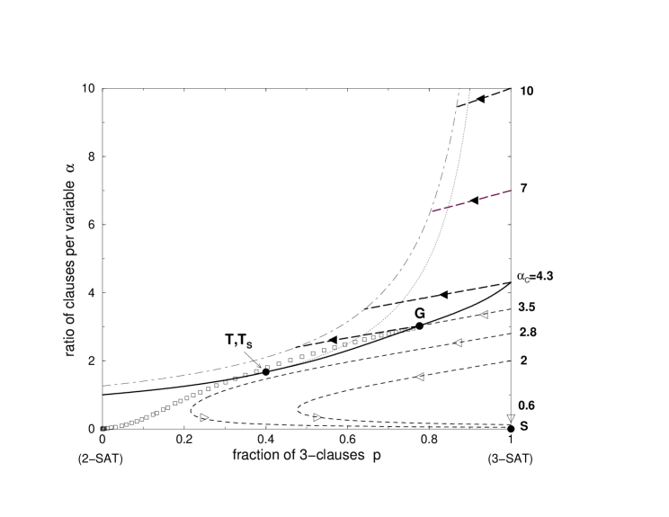
FIG. 4.: Phase diagram of the 2+p-SAT model and trajectories generated by DPLL. The threshold line $\alpha_{C}(p)$ (bold full line) separates sat (lower part of the plane) from unsat (upper part) phases. Extremities lie on the vertical 2-SAT (left) and 3-SAT (right) axis at coordinates ($p=0,\alpha_{C}=1$) and ($p=1,\alpha_{C}\simeq 4.3$) respectively. The threshold line coincides with the $\alpha=1/(1-p)$ curve (dotted line) when $p\leq p_{S}\simeq 0.41$, that is, up to the tricritical point T_S. Departure points for DPLL trajectories are located on the 3-SAT vertical axis and the corresponding values of $\alpha_{0}$ are explicitly given. Dashed curves represent tree trajectories in the unsat region (thick lines, black arrows) and branch trajectories in the sat phase (thin lines, empty arrows). Arrows indicate the direction of motion along trajectories parametrized by the fraction $t$ of variables set by DPLL. For small ratios, e.g. $\alpha_{0}=2<\alpha_{L}\simeq 3.003$, trajectories remain confined in the sat phase. At $\alpha_{L}$, the single branch trajectory hits tangentially the threshold line in T of coordinates $(2/5,5/3)$, very close to T_S. In the intermediate range $\alpha_{L}<\alpha_{0}<\alpha_{C}$, the branch trajectory intersects the threshold line at some point G that depends on $\alpha$. A dense tree then grows in the unsat phase, as happens when 3-SAT departure ratios are above threshold $\alpha>\alpha_{C}\simeq 4.3$. The tree trajectory halts on the dot-dashed curve $\alpha\simeq 1.259/(1-p)$ where the tree growth process stops. At this point, DPLL has reached back the highest backtracking node in the search tree, that is, the first node when $\alpha_{0}>\alpha_{C}$, or node G for $\alpha_{L}<\alpha_{0}<\alpha_{C}$. In the latter case, a solution can be reached from a new descending branch (rightmost path in Figure 2C) while, in the former case, unsatisfiability is proven. Small squares show the trajectory corresponding to this successful branch for $\alpha=3.5$, as obtained from simulations for $N=300$. The trajectory coincides perfectly with the theoretical branch trajectory up to point G (not shown), and then reaches the $\alpha=0$ axis when a solution is found.

FIG. 5.: Distribution of the logarithms (in base 2, and divided by $N$) of the complexity for four different sizes $N=$ 30 (dot-dashed), 50 (dashed), 100 (dotted) and 200 (full line). The histograms are normalized to unity and represent 50,000 instances. The distribution gets more and more concentrated as the size grows. A. Ratio $\alpha=10$. Curves are roughly symmetrical around their mean with small tails on their flanks; large fluctuations from sample to sample are absent. B. Ratio $\alpha=3.1$. Curves have large tails on the right, reflecting the presence of rare, very hard samples.

FIG. 6.: Complexity of solving in the sat region for $\alpha<\alpha_{L}\simeq 3.003$, divided by the size $N$ of the instances. Numerical data are for sizes $N=$50 (cross), 75 (square), 100 (diamond), 500 (triangle) and 1000 (circle). For the two biggest sizes, simulations have been carried out for ratios larger than 2.5 only. Data for different $N$ collapse onto the same curve, proving that complexity scales linearly with $N$. The bold continuous curve is the analytical prediction $\gamma(\alpha)$ from Section IV C 2. Note the perfect agreement with numerics except at large ratios where finite size effects are important, due to the cross-over to the exponential regime above $\alpha_{L}\simeq 3.003$.

FIG. 7.: Logarithm of the number of branches in unsat search trees as a function of the branch length. Main figure: the size of the search tree is a decreasing function of $\alpha$ at fixed $N$. Histograms are presented here for ratios equal to $\alpha=4.3$ (solid line, $N=200$), $\alpha=7$ (dotted line, $N=400$), $\alpha=10$ (dashed line, $N=600$) and $\alpha=20$ (dotted-dashed line, $N=900$) and have been averaged over hundreds of samples. Inset: the heights of the tops of the histograms show a very weak dependence upon $N$. Numerical extrapolations of $\omega_{N}$ to $N\to\infty$ and statistical errors are reported Table II. Sat instances (which may be present for small sizes at $\alpha=4.3$) have not be considered in the averaging procedure. For each inset, we give below the sizes $N$ followed by the number of instances in parenthesis used for averaging. Ratio $\alpha=4.3$: solid line: 100 (5000), dotted line: 150 (500), dashed line: 200 (400); $\alpha=7$: solid line: 200 (10000), dotted line: 300 (1000), dashed line: 400 (200). $\alpha=10$: solid line: 400 (500), dotted line: 500 (400), dashed line: 600 (100); $\alpha=20$: solid line: 700 (600), dotted line: 800 (1000), dashed line: 900 (1000).

FIG. 8.: Solving complexity in the upper sat phase for sizes $N$ ranging from $N=100$ to $N=400$. The size of the symbols accounts for the largest statistical error bar. A. 3-SAT problem with ratio $\alpha=3.5$: typical (average of the logarithm, full circles) and annealed (logarithm of the average, full triangles) size of the search tree. Dotted lines are quadratic and linear fit of the typical and annealed complexities, giving $\omega_{3}^{typ}=0.035\pm 0.03$ and $\omega_{3}^{ann}=0.043\pm 0.02$ in the infinite size limit. B. Related 2+p-SAT problem with parameters $p_{G}=0.78,\alpha_{G}=3.02$. The typical complexity is measured from the size of the search tree (circles) and the top of the branch length distribution (triangle), with the same large $N$ extrapolation: $\omega_{2+p}^{typ}=0.041\pm 0.02$. This value is slightly smaller than the annealed complexity $\omega_{2+p}^{ann}=0.044\pm 0.02$. All fits are linear.

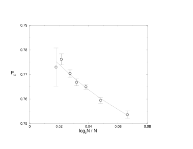
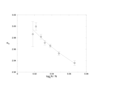
FIG. 9.: Coordinates of the highest backtracking point G in the search tree with a starting ratio $\alpha=3.5$ (the upper sat phase) for different sizes $N=100,\ldots,500$ and averaged over 10,000 (small sizes) to $128$ ($N=500$) instances. The fits shown are quadratic functions of the plotting coordinate $\log_{2}N/N$, and give the extrapolated location of $G$ in the large size limit: $p_{G}=0.78\pm 0.01$, $\alpha_{G}=\ 3.02\pm 0.02$. Note the uncertainty on these values due to the few number of instances available at large instance sizes.

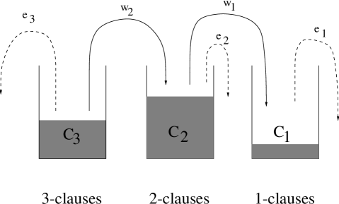
FIG. 10.: Schematic view of the dynamics of clauses. Clauses are sorted into three recipients according to their lengths, i.e. the number of variables they include. Each time a variable is assigned by DPLL, clauses are modified, resulting in a dynamics of the recipients populations (lines with arrows). Dashed lines indicate the elimination of (satisfied) clauses of lengths 1, 2 or 3. Bold lines represent the reduction of 3-clauses into 2-clauses, or 2-clauses into 1-clauses. The flows of clauses are denoted by $e_{1},e_{2},e_{3}$ and $w_{2},w_{1}$ respectively. A solution is found when all recipients are empty. The level of the rightmost recipient coincides with the number of unitary clauses. If this level is low (i.e. $O(1)$), the probability that two contradictory clauses $x$ and $\bar{x}$ are present in the recipient is vanishingly small. When the level is high (i.e. $O(\sqrt{N})$), contradictions will occur with a large probability.

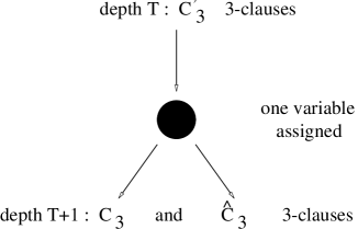
FIG. 11.: Schematic representation of the search tree building up in the toy dynamical process. A branch carrying a formula with $C^{\prime}_{3}$ 3-clauses splits once a variable is assigned, and gives birth to two branches having $C_{3}$ and $\hat{C}_{3}$ 3-clauses respectively. The variable is assigned randomly, independently of the 3-clauses. Clauses of lengths one or two are not considered.

FIG. 12.: Logarithm $\omega$ of the number of branches (base 2, and divided by $N$) as a function of the number $c_{3}$ of 3-clauses at different times $t$ for the simplified growth process of Section V A. At time $t=0$, the search tree is empty and the ratio of clauses per variable equals $\alpha_{0}=5$. Later on, the tree grows and a whole distribution of branches appears. Dominant branches correspond to the top of the distributions of coordinates $\hat{c}_{3}(t),\hat{\omega}(t)$. Branches become exponentially more numerous with time, while they carry less and less 3-clauses.

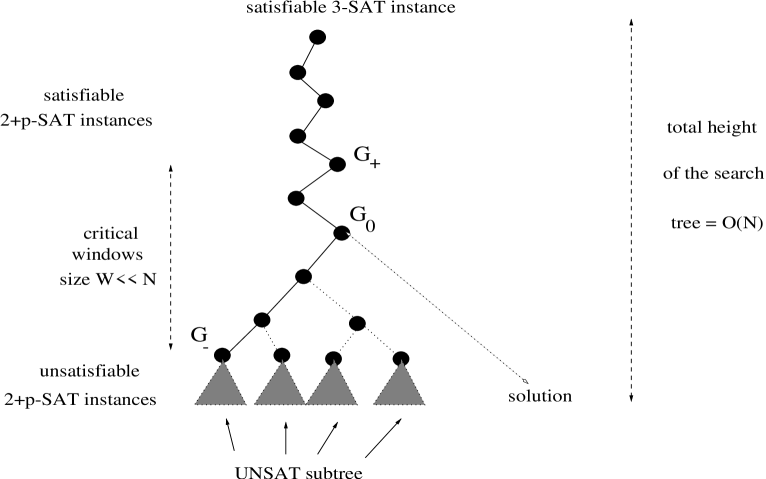
FIG. 13.: Detailed structure of the search tree in the upper sat phase ($\alpha_{L}<\alpha<\alpha_{C}$). DPLL starts with a satisfiable 3-SAT instance and transforms it into a sequence of 2+p-SAT instances. The bold, leftmost branch in the tree symbolizes the first descent made by DPLL. Above node $G_{+}$, instances are almost surely satisfiable while below $G_{-}$, instances have no solutions. The size of the critical window, that is, the number of variables to assign to reach $G_{-}$ from $G_{+}$, is $W\ll N$. $G_{0}$ denotes the highest node in the tree carrying a satisfiable 2+p-SAT instance. A grey triangle accounts for (exponentially) large refutation subtree that DPLL has to go through before backtracking above $G_{-}$. By definition, the highest node reached back by DPLL is $G_{0}$. Further backtracking, below $G_{0}$, might be necessary but a solution will be eventually found along the rightmost branch issued from $G_{0}$.

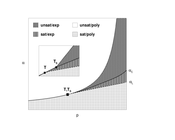
FIG. 14.: Four different regions coexist in the phase diagram of the 2+p-SAT model, according to whether complexity is polynomial or exponential, and formulae are sat or unsat. Borderlines are (from top to down): $\alpha=1/(1-p)$ (dotted line), $\alpha_{C}(p)$ (full line), and the branch trajectory (dashed line), starting in $(1,\alpha_{L})$ and ending at point T tangentially to the threshold line. The tricritical point T_S, with coordinates $p_{S}\simeq 0.41,\alpha_{S}=1/(1-p_{S})$, separates second from first order critical point on the threshold line, and lies very close to T. Inset: schematic blow-up of the T, T_S region (same symbols as in the main picture).

FIG. 15.: Sketch of the function $L(x)$ appearing in the denominator of the eigenvector generating function $\tilde{V}_{q}(x)$. $L(x)$ is positive (resp. negative) for positive (resp. negative) arguments $x$. The local positive minimum is located at $x_{m}=1/\gamma_{2},L_{m}=e\,\gamma_{2}$. The height of the minimum, $L_{m}$, is equal to the edge $\Lambda_{1}$ of the (excited states) continuous spectrum. For $\Lambda>L_{m}$, the equation $L(x)=\Lambda$ has two roots $x_{-},x_{+}$ such that $x_{-}<x_{m}<x_{+}$. When $x_{-}$ coincides with the positive zero $x^{*}$ of the numerator $N(x)$, the maximal eigenvalue $\Lambda_{0}$ is obtained (Appendix A).

FIG. 16.: Critical curves of $m_{2}=2c_{2}/(1-t)$ as a function of the parameter $y_{2}$. From bottom to top (left side): delocalization threshold $m_{2}^{loc.1}$ for the second largest eigenvector (dotted line), delocalization threshold $m_{2}^{loc.0}$ for the largest eigenvector (full line), and zero gap curve $m_{2}^{gap}$ (dashed line). All curve meet in $y_{2}=\ln 2,m_{2}=4$. For $y_{2}<\ln 2$ and small $m_{2}$, the largest eigenvector is separated from a continuum of excited states by a finite gap, and undergoes a delocalization condition when $m_{2}$ reaches $m_{2}^{loc.0}$. For $y_{2}>\ln 2$, the largest eigenvector merges with the continuum spectrum when $m_{2}\geq m_{2}^{gap}$, and gets delocalized on the critical line $m_{2}^{loc1}$.

REFERENCES

- [1] McKane, A., Droz, M., Vannimenus, J. & Wolf, D. (eds.) Scale invariance, interfaces, and non–equilibrium dynamics. (Nato Asi Series B: Physics vol. 344, Plenum Press, New-York, 1995).
- [2] Garey, M. & Johnson, D.S. Computers and Intractability; A guide to the theory of NP–completeness (W.H. Freeman and Co., San Francisco, 1979).
- [3] D.E. Knuth, “The art of computer programming”, vol. 3, “Sorting and searching”, Reading, Massachusetts: Addison-Wesley (1998).
- [4] Hayes, B. American Scientist 85(2), 108–112 (1996). (http://www.amsci.org/amsci/issues/Comsci97/compsci9703.html)
- [5] Davis, M. & Putnam, H. J. Assoc. Comput. Mach. 7, 201–215 (1960).
- [6] Crawford, J. & Auton, L. Proc. 11th Natl. Conference on Artificial Intelligence (AAAI-93), 21–27 (The AAAI Press / MIT Press, Cambridge, MA, 1993).
- [7] Cheeseman, P., Kanefsky, B., and Taylor W.M. In J. Mylopoulos and R. Reiter (eds.) Proc. of IJCAI-91, 331–337 (Morgan Kaufmann, San Mateo, CA, 1991).
- [8] Mitchell, D., Selman, B. & Levesque, H. Proc. of the Tenth Natl. Conf. on Artificial Intelligence (AAAI-92), 440-446 (The AAAI Press / MIT Press, Cambridge, MA, 1992).
- [9] Hogg, T., Huberman, B.A. & Williams, C. (eds.) Frontiers in problem solving: phase transitions and complexity. Artificial Intelligence 81(I & II) (1996).
- [10] Kirkpatrick, S. & Selman, B. Science 264, 1297–1301 (1994).
- [11] Friedgut, E., Journal of the A.M.S. 12, 1017 (1999).
- [12] Monasson, R. & Zecchina, R. Phys. Rev. E 56, 1357-1370 (1997).
- [13] Monasson, R., Zecchina, R., Kirkpatrick, S., Selman, B. & Troyansky, L. Nature 400, 133–137 (1999).
- [14] J.A. Hertz, A.S. Krogh, R.G. Palmer, “Introduction to the theory of neural computation”, SFI Studies in the Sciences of Complexity, Addison-Wesley (1991).
- [15] “Dynamics of Structural Change in Liquids” , ed. C.A. Angell and M. Goldstein, N.Y. Academy of Sciences (1986).
- [16] B. Selman, H.A. Kautz, B. Cohen, “Local search strategies for satisfiability testing”, Second DIMACS challenge on Cliques, Coloring and Satisfiability (1993).
- [17] S. Cocco, R. Monasson, “Trajectories in phase diagrams, growth processes and computational complexity: how search algorithms solve the 3-Satisfiability problem”, to appear in Phys. Rev. Lett., cond-mat/0009410 (2000).
- [18] Chao, M.T. & Franco, J. Information Science 51, 289–314 (1990).
- [19] A. Goerdt, in Proc. 7th Int. Symp. on Mathematical Foundations of Computer Science, 264 (1992); V. Chvàtal and B. Reed, in Proc. 33rd IEEE Symp. on Foundations of Computer Science, 620 (1992)
- [20] Frieze, A. & Suen, S. Journal of Algorithms 20, 312–335 (1996).
- [21] A. Kamath, R. Motwani, K. Palem and P. Spirakis, Random Structures and Algorithms 7, 59 (1995) ; O. Dubois, Theoretical Computer Science 81, 49 (1991)
- [22] S.A. Cook and D.G. Mitchell, In: Satisfiability Problem: Theory and Applications. Du, Gu and Pardalos (Eds). DIMACS Series in Discrete Mathematics and Theoretical Computer Science, Volume 35, 1997
- [23] Monasson, R. & Zecchina, R. J. Phys. A 31, 9209 (1998).
- [24] G. Biroli, R. Monasson, M. Weigt, Eur. Phys. J. B 14, 551 (2000).
- [25] D. Achlioptas, L. Kirousis, E. Kranakis, D. Krizanc, “Rigorous results for random (2+p)-SAT”, special issue of Theoretical Computer Science of NP-hardness and Phase transitions, to appear (2000).
- [26] Selman, B. & Kirkpatrick S., Artificial Intelligence 81, 273 (1996).
- [27] I.P. Gent, T. Walsh, Artificial Intelligence 70, 335 (1994).
- [28] Chvàtal, V. & Szmeredi, E. Journal of the ACM 35, 759–768 (1988).
- [29] Beame, P., Karp, R., Pitassi, T. & Saks, M. ACM Symp. on Theory of Computing (STOC98), 561–571 (Assoc. Comput. Mach., New York, 1998).
- [30] O. Kullmann, Theoretical Computer Science 223, 1-72 (1999).
- [31] A. Hartmann, M. Weigt, “Typical solution time for a vertex-covering algorithm on finite-connectivity random graphs”, to appear in Phys. Rev. Lett., cond-mat/0009417 (2000).
- [32] D.B. Wilson, ”The empirical values of the critical k-SAT exponents are wrong”, preprint arXiv:math/0005136 (2000).
- [33] C.P. Gomes, B. Selman, K. McAloon, C. Tret, “Randomization in back-track search: exploiting heavy-tailed profiles for solving hard scheduling profiles”, in Proc. AIPS-98, Pittsburgh, PA, June 1998.