A pseudo-spectral approach to inverse problems in interface dynamics

Abstract

An improved scheme for computing coupling parameters of the Kardar-Parisi-Zhang equation from a collection of successive interface profiles, is presented. The approach hinges on a spectral representation of this equation. An appropriate discretization based on a Fourier representation, is discussed as a by-product of the above scheme. Our method is first tested on profiles generated by a one-dimensional Kardar-Parisi-Zhang equation where it is shown to reproduce the input parameters very accurately. When applied to microscopic models of growth, it provides the values of the coupling parameters associated with the corresponding continuum equations. This technique favorably compares with previous methods based on real space schemes.

I Introduction

In most complex systems, it is often difficult to directly relate microscopic interactions to the dynamics of coarse-grained (mesoscale or large scale) spatial structures. In this context, nonlinear inverse methods [1] which infer equations governing a system from experimental observations of its successive time evolution, may prove to be more efficient then direct methods. When only experimental data coupled with the hypothesis of an underlying determinism are used, the identification is purely non-parametric. Such methods are extensively exploited for instance in biological and economical systems where predictions are typically relying not on basic mechanisms, but directly extrapolated from time series using various procedures (neural networks, nearest-neighbors algorithms, etc)  [1]. On the other hand if a parametrized phenomenological equation, usually derived from a combination of general symmetry considerations and heuristic physical arguments, is assumed from the outset, the inverse approach consists in finding an optimal set of parameters. In this work, we focus on this latter situation in the framework of interface growth dynamics.

The phenomenon of interface growth covers many technological applications ranging from epitaxial deposition to bacterial growth and fluid motion in porous media [2, 3, 4, 5, 6]. It is known that the large scale dynamics of such systems may be conveniently address in terms of continuum stochastic differential equations. The Kardar-Parisi-Zhang (KPZ) equation [7] constitutes a paradigmatic universality class which is believed to aggregate a large portion of observed interface dynamics. This Langevin type equation [8] possesses a non-linear term which accounts for the interface local normal growth absent in its linear counterpart the Edward-Wilkinson equation (EW) [9]. Despite a major effort both from the numerical and analytical point of view, a complete characterization of the KPZ properties is nevertheless still lacking. From the numerical viewpoint, finite-difference schemes have been widely exploited to approximate the continuum KPZ dynamics. Unfortunately, naive discretizations of the spatial derivatives may result into behaviors inconsistent with known properties of the continuum equation. For instance, the usual symmetric second-order finite difference scheme for the non-linear term violates an important symmetry of the continuum one-dimensional theory [10]. An appropriate modification in the framework of finite difference approximations may heal this drawback [10, 11], but it is nonetheless unable to properly display coarse-grained properties of the original continuum equation [12]. Specifically it does not preserve the correct functional form of the coarse-grained equilibrium distribution, a basic feature that one expects from the renormalization group point of view (a similar feature was already observed in Ref [13]).

In the present work, we follow a different route by introducing a numerical approach which preserves more features of the original continuum KPZ equation. From the outset, our method is based on a spectral rather than a finite difference scheme. Spectral methods are widely used in fluid mechanics [14] and their accuracy and reliability compared to those of finite difference schemes have been tested, over the years, on deterministic equations. Either in the context of fluctuating interfaces, it has already been used  [15, 16] to analyze the evolution of a deterministic equation, namely the Kuramoto-Shivashinsky equation. However, it has not been directly implemented on the stochastic partial differential equation [17]. In this paper, we first extend spectral methods to stochastic equations, using the KPZ equation as a testbench, then devise a reconstruction procedure for the inverse problem for the KPZ, and finally show that it is unaffected by the deficiencies of real space approximations.

The first reconstruction of the stochastic KPZ dynamics from experimental surface has been performed by Lam and Sander [18]. These authors used a standard finite-difference scheme to approximate the dynamics and based their reconstruction on a least-squares algorithm. Experimental dynamics was obtained by simulating various microscopic models. This strategy, however, seems to be limited for two reasons. First it is based on a problematic numerical approximations of the KPZ equation. Second the least-squares algorithm, originally tailored for deterministic equations was directly transpose to stochastic or Langevin type equations [18]. In fact, while the performance of this method has been tested in the presence of measurement noise - noise which affects experimental observations but does not change deterministic trajectories - in the presence of dynamical noise (e.g. Langevin dynamics) this scheme can be far more unsuccessful. Moreover, the least-squares algorithm of Ref. [18] is very much dependent on the assumption of small sampling time of observations a fact that should be checked a posteriori (see Ref. [12] for more details).

In a previous paper [12], an alternative reconstruction algorithm which does not suffer of the aforementioned problems, was introduced. The basic strategy amounts to apply the least-squares procedure at the level of correlation functions rather than directly to the interface stochastic variables. This method, albeit successful, could not correctly account for the surface coarse grained properties because of an intrinsic deficiency of spatial discretizations. Motivated by this feature, we shall remove this drawback by introducing a spectral representation of the Langevin equation which is not plagued by discretization problems. Then we shall proceed to reformulate and test the approach of Ref [12] for the inverse KPZ problem, in spectral space.

The paper is roughly divided in two parts and organized as follows. The first part concerns the KPZ equation itself and its approximations. In Section II, the continuum KPZ equation in ($1+1$)-dimension is rapidly recalled along with some previous spatial discretizations used to numerically mimic it. In the same Section, a novel discretization in Fourier space is then proposed and shown to improve over the real space approach from a purely theoretical viewpoint. The deterministic evolution equation for correlations functions in spectral space, are then derived in Section III. Section IV is devoted to the numerical procedure and, in particular, to the treatment, via a pseudo-spectral method, of the nonlinear term of the KPZ equation. Numerical results are then provided to compare the performance of the various discretizations to the corresponding analytical results obtained for the continuum KPZ equation. The second part of the paper is devoted to the inverse method for KPZ dynamics, where we discuss how one can reconstruct the dynamics from the knowledge of interface profiles. This technique, based on equations derived in Section III, is described in Section V. It is then tested in Section VI against data produced by synthetic interface profiles generated by a ($1+1$)-dimensional KPZ equation with known coupling parameters. The test is performed even in the presence of coarse-graining and provides the renormalization properties of the KPZ coupling parameters. Finally, in Section VII, the reconstruction method is applied to various microscopic models at various coarse-grained scales.

II Spectral discretization of the KPZ equation

We consider a one-dimensional surface profile of width $L$. The surface can be either experimentally or numerically generated, and we assume it to be periodic with period $L$. At a mesoscopic scale, it can be described within a continuum (hydrodynamic) approximation by a variable $h(x,t)$ (with $0\leq x\leq L$) which satisfies a Langevin equation [2]. A paradigmatic example is given by the Kardar-Parisi-Zhang (KPZ) equation [7]:

$$\partial_{t}h = c+\nu\partial_{x}^{2}h+\frac{\lambda}{2}(\partial_{x}h)^{2}+\eta,$$ (1)

where $\eta(x,t)$ is a noise with zero average and $\delta$-correlated both in time and space as:

$$\left\langle\eta(x,t)\eta(x^{\prime},t^{\prime})\right\rangle = 2D\delta(x-x^{\prime})~{}\delta(t-t^{\prime}).$$ (2)

In Eq. (1), symbol $\left\langle\ldots\right\rangle$ means that an ensemble average over the noise is performed and $c$, $\nu$, $\lambda$, and $D$ are coupling parameters. In writing Eqs.(1) and (2), an appropriate regularization is always tacitly assumed. This amounts to define a minimal length scale $a$ for $h(x,t)$ and to assume that the surface variable $h(x,t)$ satisfies a KPZ regularized equation with a given spatial cut-off depending on scale $a$. For instance, this can be done by considering a discretization version of Eqns. (1) and (2) with $a$ as a lattice constant :

$$\frac{dh_{i}}{dt} = c+\frac{\nu}{a^{2}}F_{i}^{\nu}[h]+\frac{\lambda}{2a^{2}}\bar{F}_{i}^{\lambda}[h]+\sqrt{\frac{D}{a}}\theta_{i},$$ (3)

or alternatively

$$\frac{dh_{i}}{dt} = c+\frac{\nu}{a^{2}}F_{i}^{\nu}[h]+\frac{\lambda}{2a^{2}}F_{i}^{\lambda}[h]+\sqrt{\frac{D}{a}}\theta_{i},$$ (4)

where $h_{j}$ stands for the value $h(x_{j},t)$ of the periodic smoothed surface at $x_{j}=ja$, $j=1,\ldots,N$ where $N=L/a$ and the quantities $\theta_{i}(t)$ are uncorrelated white noise functions

$$\left\langle\theta_{i}(t)\theta_{j}(t^{\prime})\right\rangle = 2\delta_{ij}\delta(t-t^{\prime})~{}.$$ (5)

In Eqs. (3) and (4), one usually approximate the discretized Laplacian with the second-order finite difference term

$$F_{i}^{\nu}[h] = h_{i+1}+h_{i-1}-2h_{i},$$ (6)

and the non-linear term with

$$\bar{F}_{i}^{\lambda}[h] = \frac{1}{4}\bigl{[}h_{i+1}-h_{i-1}\bigr{]}^{2},$$ (7)

or

$$F_{i}^{\lambda}[h] = \frac{1}{3}\bigl{[}(h_{i+1}-h_{i})^{2}+(h_{i}-h_{i+1})^{2}$$ (8)

$$+ (h_{i+1}-h_{i})(h_{i}-h_{i-1})\bigr{]}.$$ (9)

As previously discussed  [10, 11, 12], only choice given by Eq. (9) guarantees that at least some properties of the correct equilibrium distribution are retrieved. Both representations Eqs. (7) and  (9) are however problematic at the coarse-grained level [12].

Here we show how one can achieve an alternative and always correct discretization of the continuum KPZ equation by a procedure that directly applies in momentum space.

We first expand the periodic continuum field $h(x,t)$ in Fourier modes as

$$h(x,t) = \frac{1}{L}\sum_{n=-\infty}^{+\infty}\widehat{h}_{q_{n}}(t)~{}e^{iq_{n}x},$$ (10)

where the Fourier component

$$\widehat{h}_{q_{n}}(t) = \int_{-L/2}^{L/2}~{}dx~{}h(x,t)~{}e^{-iq_{n}x},$$ (11)

is associated with wavenumber $q_{n}=2\pi n/L$. Since $h(x,t)$ is real, this imposes $\widehat{h}_{q_{n}}^{*}=\widehat{h}_{-q_{n}}$ or alternatively, if $\widehat{h}_{q_{n}}=\widehat{\alpha}_{q_{n}}+i\widehat{\beta}_{q_{n}}$ is separated in real and imaginary part, $\widehat{\alpha}_{-q_{n}}=\widehat{\alpha}_{q_{n}}$, $\widehat{\beta}_{-q_{n}}=-\widehat{\beta}_{q_{n}}$. A similar expansion for the noise term $\eta(x,t)$ leads to Fourier components $\widehat{\eta}_{q_{n}}$ with the following correlations :

$$\left\langle\widehat{\eta}_{q_{n}}(t)\widehat{\eta}_{q_{m}}(t^{\prime})\right\rangle = 2DL\delta_{n,-m}\delta(t-t^{\prime}).$$ (12)

Again by decomposing Fourier modes $\widehat{\eta}_{q_{n}}\equiv\widehat{\xi}_{q_{n}}+i\widehat{\zeta}_{q_{n}}$ in their real and imaginary parts, one obtains, in addition to relations $\widehat{\xi}_{q_{n}}=\widehat{\xi}_{q_{-n}}$, $\widehat{\zeta}_{q_{n}}=-\widehat{\zeta}_{q_{-n}}$, conditions on the correlations

$$\left\langle\widehat{\xi}_{q_{n}}(t)\widehat{\xi}_{q_{m}}(t^{\prime})\right\rangle = DL\delta_{n,m}\delta(t-t^{\prime}),$$ (13)

$$\left\langle\widehat{\zeta}_{q_{n}}(t)\widehat{\zeta}_{q_{m}}(t^{\prime})\right\rangle = DL\delta_{n,m}\delta(t-t^{\prime}),$$ (14)

$$\left\langle\widehat{\xi}_{q_{n}}(t)\widehat{\zeta}_{q_{m}}(t^{\prime})\right\rangle = 0,$$ (15)

for $n>0$,$m>0$. For the Fourier component $n=0$, one gets $\widehat{\zeta}_{q_{0}}=0$ and

$$\left\langle\widehat{\xi}_{q_{0}}(t)\widehat{\xi}_{q_{0}}(t^{\prime})\right\rangle = 2DL\delta(t-t^{\prime})$$ (16)

Using Eq. (10) in Eq. (1), an infinite system of coupled Langevin equations is obtained :

$$\frac{d\widehat{h}_{q_{n}}(t)}{dt} = cL\delta_{n,0}-\nu q_{n}^{2}~{}\widehat{h}_{q_{n}}(t)$$ (17)

$$- \frac{\lambda}{2L}\sum_{m,m^{\prime}=-\infty}^{\infty}q_{m}q_{m^{\prime}}\widehat{h}_{q_{m}}(t)\widehat{h}_{q_{m^{\prime}}}(t)\delta_{n,m+m^{\prime}}+\widehat{\eta}_{q_{n}}(t).$$ (18)

The spectral approximation now amounts to project the above infinite system on the space of periodic functions of period $L$ with a finite number of Fourier modes $\widehat{h}_{q_{n}}$ ($|q_{n}|\leq q_{N/2}$). All equations retain their original form with the proviso that infinite sums $\sum_{n=-\infty}^{\infty}$ are now replaced by finite ones $\sum_{n=-N/2}^{N/2}$. This procedure thus assumes that $\widehat{h}_{q_{n}}=0$ for any $n>N/2$, and the original continuum equation is then reduced to a set of $N+1$ real Langevin equations. The first one

$$\frac{d\widehat{h}_{q_{0}}}{dt} = cL+\frac{\lambda}{L}\sum_{n=1}^{N/2}q_{n}^{2}\Bigl{[}\widehat{\alpha}_{q_{n}}^{2}+\widehat{\beta}_{q_{n}}^{2}\Bigr{]}+\widehat{\xi}_{q_{0}},$$ (19)

governs the temporal evolution of the zeroth mode $\widehat{h}_{q_{0}}$ and depends on $\widehat{h}_{q_{n}}$ for $0<n\leq N/2$. The other $N$ real equations are independent of $\widehat{h}_{q_{0}}$ and describe the time evolution of $\widehat{\alpha}_{q_{1}}$, $\widehat{\beta}_{q_{1}}$,$\ldots$, $\widehat{\alpha}_{q_{N/2}}$,$\widehat{\beta}_{q_{N/2}}$ :

$$\frac{d\widehat{\alpha}_{q_{n}}}{dt} = F_{q_{n}}\Bigl{[}\widehat{\alpha},\widehat{\beta}\Bigr{]}+\widehat{\xi}_{q_{n}},$$ (20)

$$\frac{d\widehat{\beta}_{q_{n}}}{dt} = G_{q_{n}}\Bigl{[}\widehat{\alpha},\widehat{\beta}\Bigr{]}+\widehat{\zeta}_{q_{n}},$$ (21)

where

$$F_{q_{n}}\Bigl{[}\widehat{\alpha},\widehat{\beta}\Bigr{]} = -\nu q_{n}^{2}\widehat{\alpha}_{q_{n}}$$ (22)

$$- \frac{\lambda}{2L}\sum_{m,m^{\prime}=-N/2}^{N/2}q_{m}q_{m^{\prime}}\Bigl{[}\widehat{\alpha}_{q_{m}}\widehat{\alpha}_{q_{m^{\prime}}}-\widehat{\beta}_{q_{m}}\widehat{\beta}_{q_{m^{\prime}}}\Bigl{]}\delta_{n,m+m^{\prime}},$$ (23)

$$G_{q_{n}}\Bigl{[}\widehat{\alpha},\widehat{\beta}\Bigr{]} = -\nu q_{n}^{2}\widehat{\beta}_{q_{n}}$$ (24)

$$- \frac{\lambda}{2L}\sum_{m,m^{\prime}=-N/2}^{N/2}q_{m}q_{m^{\prime}}\Bigl{[}\widehat{\alpha}_{q_{m}}\widehat{\beta}_{q_{m^{\prime}}}+\widehat{\beta}_{q_{m}}\widehat{\alpha}_{q_{m^{\prime}}}\Bigl{]}\delta_{n,m+m^{\prime}}.$$ (25)

The philosophy underlying this regularization is akin a renormalization group scheme in momentum space, where high wavevectors are integrated out above a cut-off $q_{N/2}$ in momentum space. This approximation is an alternative - albeit not equivalent - method to discretize, in real space, the width $L$ into $N+1$ independent points separated by a distance $a=L/N$. For the sake of simplicity, the number $N$ is hereafter assumed to be a power of two.

For the continuum linear counterpart - the EW equation - no approximations are involved in the framework of this spectral method, as equations for modes $q_{n}>q_{N/2}$ are simply discarded. On the other hand, this approach is shown to be far more useful than the real space Eqs. (3) and (4), in the non-linear KPZ case, since it preserves, unlike both approximations given in Eqs. (3) and (4), some basic properties of the original KPZ continuum equation as shown below. Indeed let us recall that, apart from a normalization factor, the steady state distribution of continuum KPZ is given by

$$P_{s}[h] \sim \exp\biggl{[}-\frac{\nu}{2D}\int_{-L/2}^{L/2}~{}dx\bigl{(}\partial_{x}h\bigr{)}^{2}\biggr{]}.$$ (26)

The distribution of modes $|q_{n}|\leq q_{N/2}$ in momentum space thus reads :

$$P_{s}[\widehat{h}_{q_{1}},..,\widehat{h}_{q_{N/2}}] \sim \exp\biggl{[}-\frac{\nu}{2LD}\sum_{n=-N/2}^{N/2}q_{n}^{2}|\widehat{h}_{q_{n}}|^{2}\biggr{]}.$$ (27)

The zeroth mode $\widehat{h}_{q_{0}}$ does not contribute to (27) since the average value of $h(x,t)$ does not appear in (26), meaning that the surface always grows and its average never settles to a steady value unlike surface gradients. We note that both the original distribution Eq. (26) and its spectral approximation Eq. (27) are independent of $\lambda$. As already remarked in Ref.  [10], this property is not satisfied by the finite difference approximation Eq. (3). This inconvenient point is partly solved by the modification given in Eq.  (4) which leads to the correct steady state distribution

$$P_{s}[h_{1},\ldots,h_{N}] \sim \exp\biggl{[}-\frac{\nu}{2Da}\sum_{j=1}^{N}({h_{j+1}-h_{j}})^{2}\biggr{]}.$$ (28)

However it has been shown in Ref. [12], that even the approximation given in Eq. (4), fails in the presence of coarse-graining. This means that if fluctuating interfaces, obtained by the numerical generation of a real space discretized KPZ equation at scale $a$, are smoothed out up to a scale $a_{s}>a$, these coarse-grained surfaces cannot be described by a renormalized KPZ equation at $a_{s}$. The origin of this problem can be traced back to the form of the steady state distribution (28) within a real space scheme. On the contrary, our spectral discretization has been devised in such a way to avoid this drawback (see below), and can then act as a safe starting point for the reconstruction procedure.

On remembering that there are only $N$ independent modes, the Fokker-Planck equation governing the evolution of the probability distribution $P[\widehat{\alpha},\widehat{\beta},t]$ associated with the Langevin equations  (20)-(21), reads [8]:

$$\frac{\partial P}{\partial t} = \sum_{n=1}^{N/2}[-\frac{\partial(F_{q_{n}}P)}{\partial\widehat{\alpha}_{q_{n}}}-\frac{\partial(G_{q_{n}}P)}{\partial\widehat{\beta}_{q_{n}}}+\frac{DL}{2}(\frac{\partial^{2}P}{\partial\widehat{\alpha}_{q_{n}}^{2}}+\frac{\partial^{2}P}{\partial\widehat{\beta}_{q_{n}}^{2}})].$$ (29)

One may then check that the steady solution (27) satisfies  Eq. (29). It is known [8] that, when such a steady probability exists, all time dependent distributions asymptotically converge towards it. The discretized KPZ thus preserves the particular symmetry of the continuum KPZ equation. A further advantage of this discretization, is that surfaces coarse-grained at length scales $a_{s}>a$ can be simply obtained by cutting out modes with wavenumber larger than $q_{{N_{s}}/2}$ ($N_{s}=Na/a_{s}$). From Eq.  (29), it is straightforward to get the steady probability of these coarse-grained surfaces, that is a steady probability of the same form as equation (27) with $N=N_{s}$ and the same $\frac{D}{\nu}$ ($L=N_{s}a_{s}$). The coupled Langevin equations (20) and (21), ensure that, under coarse-graining, the exact steady-state is recovered.

III Evolution equations for correlation functions.

Next we address the time dependent distribution $P[\widehat{\alpha},\widehat{\beta},t]$ appearing in equation (29). We first exhibit an evolution equation for the ensemble average $\left\langle\widehat{\alpha}_{q_{n}}^{2}\right\rangle(t)$, and $\left\langle\widehat{\beta}_{q_{n}}^{2}\right\rangle(t)$

$$\left\langle\widehat{\alpha}_{q_{n}}^{2}\right\rangle(t) = \int{\cal D}\widehat{\alpha}{\cal D}\widehat{\beta}~{}\widehat{\alpha}_{q_{n}}^{2}~{}P[\widehat{\alpha},\widehat{\beta},t],$$ (30)

$$\left\langle\widehat{\beta}_{q_{n}}^{2}\right\rangle(t) = \int{\cal D}\widehat{\alpha}{\cal D}\widehat{\beta}~{}\widehat{\beta}_{q_{n}}^{2}~{}P[\widehat{\alpha},\widehat{\beta},t],$$ (31)

where

$${\cal D}\widehat{\alpha}{\cal D}\widehat{\beta} = \prod_{j=1}^{N/2}~{}d\widehat{\alpha}_{q_{j}}~{}d\widehat{\beta}_{q_{j}}.$$ (32)

Assume that the probability density $P[\widehat{\alpha},\widehat{\beta},t]$ goes exponentially to zero for $\widehat{\alpha}$, $\widehat{\beta}$ going to $\infty$. If the Fokker Planck equation (29) is multiplied by $\widehat{\alpha}^{2}_{q_{n}}$ and then integrated over all variables, one obtains, after an integration by parts :

$${\frac{d\left\langle\widehat{\alpha}_{q_{n}}^{2}\right\rangle(t)}{dt}} = 2\int~{}{\cal D}\widehat{\alpha}{\cal D}\widehat{\beta}~{}\widehat{\alpha}_{q_{n}}F_{q_{n}}[\widehat{\alpha},\widehat{\beta}]P[\widehat{\alpha},\widehat{\beta},t]+DL,$$ (33)

and similarly for $\widehat{\beta}_{q_{n}}^{2}(t)$,

$${\frac{d\left\langle\widehat{\beta}_{q_{n}}^{2}\right\rangle(t)}{dt}} = 2\int~{}{\cal D}\widehat{\alpha}{\cal D}\widehat{\beta}~{}\widehat{\beta}_{q_{n}}G_{q_{n}}[\widehat{\alpha},\widehat{\beta}]P[\widehat{\alpha},\widehat{\beta},t]+DL.$$ (34)

From the expressions (23)-(25), we then get for $n>0$

$$\frac{d}{d~{}t}\left\langle|\widehat{h}_{q_{n}}|^{2}\right\rangle = -2\nu q_{n}^{2}\left\langle|\widehat{h}_{q_{n}}|^{2}\right\rangle-\lambda{\cal V}_{q_{n}}+2DL,$$ (35)

where

$${\cal V}_{q_{n}} = \frac{1}{L}\sum_{m,~{}m^{\prime}=-N/2}^{N/2}q_{m}~{}q_{m^{\prime}}{\cal R}\Bigl{[}\left\langle\widehat{h}_{-q_{n}}\widehat{h}_{q_{m}}\widehat{h}_{q_{m^{\prime}}}\right\rangle\Bigr{]}\delta_{n,m+m^{\prime}},$$ (36)

and ${\cal R}$ indicates that only the real part is considered. Equation (35) implies that

$$\frac{d}{dt}g_{2}(t) = -2\nu g_{4}(t)-\lambda K(t)+2DQ_{2},$$ (37)

where

$$g_{2p}(t) \equiv \frac{1}{L}\sum_{n=-N/2}^{N/2}q_{n}^{2p}\left\langle|\widehat{h}_{q_{n}}(t)|^{2}\right\rangle,$$ (38)

for $p=1,2,\ldots$ and

$$K(t) = \frac{1}{L^{2}}\sum_{n,m,m^{\prime}=-N/2}^{N/2}q_{n}^{2}q_{m}q_{m^{\prime}}$$ (40)

$${\cal R}\Bigl{[}\left\langle\widehat{h}_{-q_{n}}(t)\widehat{h}_{q_{m}}(t)\widehat{h}_{q_{m^{\prime}}}(t)\right\rangle\Bigr{]}\delta_{n,m+m^{\prime}},$$

$$Q_{2} = \sum_{n=-N/2}^{N/2}q_{n}^{2}=\frac{4}{3}\pi^{2}\frac{N(N+1)(2N+1)}{L^{2}}.$$ (41)

In Appendix A is shown that the term $K(t)$ in Eq. (37) actually vanishes identically. Hence one is left with

$$\frac{d}{dt}g_{2}(t) = -2\nu g_{4}(t)+2DQ_{2}.$$ (42)

Therefore only $\nu$ and $D$ explicitly appear in the above equation. The absence of the parameter $\lambda$ in Eq. (42) is reminiscent of an analogous phenomenon appearing in the steady probability distribution (27) in $1+1$ dimensional case. It is worth stressing that, although the $\lambda$ term does not explicitly appear in Eq. (42), it is nevertheless implicitly present through the evolution of $g_{4}(t)$.

Another equation can be obtained by averaging Eq. (19)

$$\frac{d}{dt}g_{0}(t) = cL+\frac{\lambda}{2}g_{2}(t).$$ (43)

where

$$g_{0}(t) \equiv \left\langle\widehat{h}_{q_{0}}(t)\right\rangle,$$ (44)

This latter relation does not explicitly involve either the noise or the diffusion term.

IV The Pseudo-spectral method for the KPZ equation

A Numerical procedures

In order to compare rough surfaces numerically generated by various spatial discretizations of the KPZ equation, we introduce a one step Euler Scheme in time for the temporal discretization. This simple algorithm is used since, for stochastic equations, it is known that a naive application of a two-steps method can result in less computational efficiency  [19]. In order to speed up the evolution of equations (20) and (21), a pseudo-spectral method is used at each time step of the Euler scheme. This method efficiently computes the quantity

$$\widehat{\chi}_{q_{n}} = -\frac{\lambda}{2L}\sum_{m,m^{\prime}=-N/2}^{N/2}q_{m}q_{m^{\prime}}\widehat{h}_{q_{m}}(t)\widehat{h}_{q_{m^{\prime}}}(t)\delta_{n,m+m^{\prime}},$$ (45)

whose real and imaginary part are the non-linear contributions of the $N+1$ Langevin equations  (20) and (21). In this procedure, quantity $\widehat{\chi}_{q_{n}}$ can be evaluated without explicitly performing the double sum appearing in Eq. (45) for each $n$. First, the Fourier modes of the surface derivative $\partial_{x}h(x,t)$ are obtained by a simple algebraic multiplications $iq_{n}\widehat{h}_{q_{n}}$ for $0\leq n\leq N/2$. One then returns to real space

$$\partial_{x}h(x,t)=\frac{1}{L}\sum_{n=-N/2}^{N/2}iq_{n}\widehat{h}_{q_{n}}(t)~{}e^{{i}q_{n}x}.$$ (46)

to obtain the gradient at given spatial points. The computation of $\frac{\lambda}{2}(\partial_{x}h)^{2}$ is then straightforward at these points. One then exploits again a Fourier transform to go back to spectral space using the values of the nonlinear terms at these collocation points. In order to prevent the aliasing problem  [14],  [20], we suitably choose the range of the collocation points and the number of Fourier modes to be used, in such a way that the procedure provides the exact $\widehat{\chi}_{q_{n}}$ for $0\leq n\leq N/2$ of Eq. (45). The modes external to the range $-N/2\leq n\leq N/2$ can be dropped since they do not enter in the actual computations. This well-known technique (dealiasing [14]), albeit seemingly more complicated, turns out to be much more efficient of a brute force computation of Eq. (45).

B Comparison with real space discretization

We now compare the performance of the spectral discretization with the one based on the standard Eq.  (3) and modified Eq. (4) real space discretization and with the corresponding analytical results obtained for the continuum KPZ equation. The surface is grown via the pseudo-spectral KPZ equations with a regularization at scale $a$. In these simulations we have always used an Euler time step in the range $10^{-2}-10^{-3}$ which is sufficiently small to avoid any numerical instability up to the sizes and for the $\lambda$ considered in here.

In order to compare the performances of the pseudo-spectral method with respect to the real space discretization schemes, we apply a test akin to the one carried of in Ref. [11]. We generate a steady state KPZ surface in ($1+1$) dimension, with lattice spacing $a=1$, and parameters $\nu=1$, $\lambda=3$, $D=1$, $c=0$, by using (i) the standard real space discretization (3), (ii) the real space discretization (4) introduced in Ref. [11], (iii) our pseudo-spectral discretization. The steady state roughness $W(L)$ obtained by the three methods for various sizes $L$ is then compared with the exact value

$$W(L) = \sqrt{\frac{D}{12\nu}}L^{1/2},$$ (47)

of the continuum KPZ equation [21]. Fig. 1 shows that, unlike the standard real space representation (3) which underestimates the ratio $\nu/D$ ($=1$ in the present case), both the modified real space representation (4) and the pseudospectral representation yield, on average, the correct ratio. This is no surprise since we have previously shown that the pseudo-spectral representation correctly accounts for the steady-state distribution properties, a feature not shared by of the standard real space representation  (3) [12].

Figure 2 depicts the behavior of $g_{2}(t)$ for a surface of a size $L=256$, flat at $t=0$, and average over ${\cal N}=500$ independent growths. The curve has a gradual increase (starting from zero) until it saturates after a characteristic time $t_{\infty}^{\mathbf{c}}\sim 30000\times 10^{-3}$ This time, which depends upon the size of the system, represents the cross-over after which (i) all length scales have saturated, (ii) the velocity of the average height becomes constant and (iii) the roughness levels off. From renormalization group theory, one expects that $t_{\infty}^{\mathbf{c}}\sim L^{z}$ where the dynamical exponent $z$ is equal to $3/2$ for $1+1$ dimension [2].

In the spirit of renormalization group theory, let us separate the dynamics of modes of wavelength shorter than $a_{s}=ba$ with $b=2^{l}$ with modes of wavelength longer than $a_{s}$. This can be done using the following decomposition of $g_{2p}(t)$ ( $N_{s}=N/b$)

$$g_{2p}(t) = g_{2p}^{(b)}(t)+R_{2p}^{(b)}(t),$$ (48)

with

$$g_{2p}^{(b)}(t) = \frac{1}{L}\sum_{n=-N_{s}/2}^{N_{s}/2}q_{n}^{2p}\left\langle|\widehat{h}_{q_{n}}(t)|^{2}\right\rangle.$$ (49)

representing the “slow” part, and

$$R_{2p}^{(b)}(t) \equiv \frac{1}{L}\sum_{n=-{N}/2}^{-N_{s}/2-1}q_{n}^{2p}\left\langle|\widehat{h}_{q_{n}}(t)|^{2}\right\rangle$$ (50)

$$+ \frac{1}{L}\sum_{n={N_{s}}/2+1}^{N/2}q_{n}^{2p}\left\langle|\widehat{h}_{q_{n}}(t)|^{2}\right\rangle,$$ (51)

indicating the “fast” part. In Fig. 3, the behavior of $g_{2}(t)$ , $g_{2}^{(b)}(t)$ and $R_{2}^{(b)}(t)$ are plotted for a scaling $b=2$. Before a characteristic time $t_{1}^{\mathbf{c}}$ ( $t_{1}^{\mathbf{c}}\sim 350\times 10^{-3}$ for the parameters chosen in the pseudo-spectral KPZ equations), shortwave modes $N_{s}/2+1\leq|n|\leq N/2$ contained in $R_{2}^{(2)}(t)$ are evolving much faster than longwave modes $0\leq|n|\leq N_{s}/2$. Similar features occur for higher values of $b=2^{l}$ thus defining a sequence of characteristic times $t_{1}^{\mathbf{c}}<t_{2}^{\mathbf{c}}<t_{3}^{\mathbf{c}}<\ldots$. For instance it is found that $t_{2}^{c}\sim 1300\times 10^{-3}$ and $t_{3}^{c}\sim 3000\times 10^{-3}$. The above remarks are clearly important when defining the dynamics of the coarse-grained surface obtained by eliminating the modes of wavelength shorter than scale $a_{s}=ba=2^{l}a$. This surface is characterized by the same average height $g_{0}^{(b)}=g_{0}$ for any $b$, and $g_{2}^{(b)}(t)$ playing the role of $g_{2}(t)$. By rewriting Eq. (43) as

$$\frac{dg_{0}^{(b)}(t)}{dt} = c\biggl{[}1+\frac{\lambda}{2L}R_{2}^{(b)}\biggr{]}L+\frac{\lambda}{2}g_{2}^{(b)}(t),$$ (52)

it is clear that the coarse-grained surface with $N_{s}=N/b$ modes will satisfy a KPZ equation with a renormalized $c_{s}$ and identical $\lambda_{s}=\lambda$ only when $R_{2}^{(b)}$ has reached saturation. On starting from a flat interface, this happens whenever the Fourier modes $N_{s}/2<n<N/2$ and $-N/2<n<-N_{s}/2$ are thermalized, i.e. for $t>t_{l}^{c}$. Similarly, upon summing Eq. (35) over the slow modes $n=1,\ldots,N_{s}/2$, one finds that,

$$\frac{dg_{2}^{(b)}(t)}{dt} = -2\nu g_{4}^{(b)}(t)-\lambda\sum_{n=-N_{s}/2}^{N_{s}/2}q_{n}^{2}{\cal V}_{q_{n}}+2DQ^{(b)}_{2},$$ (53)

where

$$Q^{(b)}_{2} = \sum_{n=-N_{s}/2}^{N_{s}/2}q_{n}^{2}.$$ (54)

For $t\geq t_{1}^{\mathbf{c}}$, it is assumed that dynamics of fast modes is slaved to the one of slow modes, in such a way that the term in $\lambda$ can be written as

$$\lambda\sum_{n=-N_{s}/2}^{N_{s}/2}q_{n}^{2}{\cal V}_{q_{n}}=2\Delta\nu g_{4}^{(b)}(t)-2\Delta DQ^{(b)}_{2},$$ (55)

thus satisfying a coarse-grained KPZ equation with renormalized parameters $\nu_{s}=\nu+\Delta\nu$ and $D_{s}=D+\Delta D$. For the EW universality class, it is easy to show that, using Eq. (52) and Eq. (53), all parameters do not renormalize, as expected from renormalization group theory [5].

Our purpose here is to compute the KPZ renormalized parameters directly from the experimental observations of the surface growth. According to the previous discussion, we should begin collecting the data after a time $t\geq t_{l}^{\mathbf{c}}$ (starting from an initially flat surface) in order to best characterize the dynamics of a surface coarse-grained by a factor $b=2^{l}$. Moreover the most prominent evolution of this surface occurs during the time interval when the length scales between $2a_{s}$ and $a_{s}=ba$ are not thermalized i.e. during the interval $[t_{l}^{\mathbf{c}},t_{l+1}^{\mathbf{c}}]$ which is then the optimal period to characterize its dynamics.

V The reconstruction procedure based on the spectral approximation.

Based upon the above spectral approximation, we now introduce a method to identify, at a given length scale, an optimal set of KPZ effective coupling parameters $c$, $\nu$, $\lambda$ and $D$, from ”experimental” snapshots of interface profiles. The ”experimental” data may be generated by numerical simulations of the KPZ equation itself (see tests in section VI), by numerical microscopic models emulating surface processes (Section VII) or associated with real interface growth. For the sake of simplicity, measurements are always assumed free of observational noise. This approach thus constitutes a typical inverse problem for an infinite (or finite, but large, in the discretized approximation) dimensional system with a finite number of parameters to identify. Although in this work we focus on the KPZ universality class, our method has a more general validity, and may be extended, with slight changes, to other universality classes.

A first reconstruction of KPZ dynamics was attempted by Lam and Sanders [18]. These authors used equation (3) and worked in real space using experimental heights $h_{i}^{obs}(t)$ measured at $N$ points $x_{j}=ja$ with $j=1,...N$. For the reconstruction, they performed a least-squares calculation directly on the Langevin equations to compute the parameters $c$, $\nu$, $\lambda$. The noise term $D$ was eventually obtained as a by product of the previous calculation. In Ref. [12], the difficulties associated with this approach have already been discussed. In the present work, the analysis is based on the philosophy explained in previous Sections and equations (42), respectively (43), are used to identify through a least-squares procedure the coefficients $\nu$, $D$, respectively $c$, $\lambda$. Besides the fundamental theoretical features discussed in Sec. II, several reasons may be invoked in favor of our approach. First, this method is not directly based on the primitive stochastic equations but uses the deterministic equations introduced in Section III which govern the ensemble average of correlation functions. Standard identification algorithms (e.g. the least-squares method) which are well suited and have been widely tested for deterministic equations, are then expected to be more reliable under such conditions. Second, as functions $g_{2p}(t)$ are already averaged quantities, a smaller number of realizations is expected to be required due to the self-averaging property. Finally, dynamical noise is directly introduced in our reconstruction algorithm, unlike in the one of Ref. [18]. This seems a natural requirement since noise is an intrinsic parameter of the interface evolution.

In order to get ensemble averages of spatial correlations, ${\cal N}$ growths starting from the same surface, e.g. a flat surface, have been carried out. This provides ${\cal N}$ distinct realizations of the same stochastic process. For a given realization, the experimental surface is observed at time $\left(t_{k}=k\Delta t,k=1,2,..,pM\right)$ where $\Delta t$ is the measurement sampling time. This procedure may be easily performed in a real experiment and leads to quantities $g_{0}(t)$, $g_{2}(t)$ and $g_{4}(t)$ which are linked, at the scale considered, to the average height, the average of the square of the first or second surface derivatives of the smoothed surface.

Let us now integrate equation (42) during $p$ sampling times $\Delta t$ :

$${\frac{g_{2}(T_{k+1})-g_{2}(T_{k})}{T_{k+1}-T_{k}}} = -2\nu{\frac{1}{T_{k+1}-T_{k}}}\int_{T_{k}}^{T_{k+1}}g_{4}(t)dt+2DQ_{2},$$ (56)

where time $T_{k}=kp\Delta t$, $(k=1,\ldots,M)$. Similarly from equation (43) one gets

$${\frac{g_{0}(T_{k+1})-g_{0}(T_{k})}{T_{k+1}-T_{k}}} = cL+\frac{\lambda}{2}\frac{1}{T_{k+1}-T_{k}}\int_{T_{k}}^{T_{k+1}}g_{2}(t)dt.$$ (57)

If $\Delta t$ is smaller than the characteristic time of the dynamics, one may approximate the time integral in Eqs. (56) and (57), as an average over the $p$ intermediate sampling times, thereby obtaining $M-1$ linear constraints on the parameters $\nu$, $D$ and $c$, $\lambda$. A simple least-squares calculation then determines $\nu$, $D$ from Eq. (56) and $c$, $\lambda$ from Eq. (57).

VI Results on the KPZ reconstruction

In order to test our reconstruction method, we use the above procedure on rough surfaces generated through a discretized KPZ equation with known coupling parameters ($\nu=1$,$\lambda=3$,$D=1$, $c=0$). Note that, in order to compute the ensemble average values $g_{0}(t)$, $g_{2}(t)$ and $g_{4}(t)$, we use ${\cal N}=500$ samples to obtain a convergent value. This is important since statistical fluctuations may be large enough to induce a measurement error exceeding the non-linear contributions, and under such circumstances the identification would fail. Furthermore each reconstruction is repeated for a small number of independent configurations (typically $5$) in order to get an estimate of the error bars associated with the reconstructed parameters.

In the absence of coarse-graining, data are produced by the discretized equations (19)-(20)- (21) where the minimum length scale $a=L/N$ is introduced by the spectral approximation. Since equations used in the reconstruction procedure are exactly identical to the ones generating the time series, this provides a first stringent test on the validity of our method. For the original data, the most efficient interval choice to perform the identification is expected to be $[0,t_{1}^{\mathbf{c}}]$. Indeed, after $t_{1}^{\mathbf{c}}$, all length scales between $a$ and $2a$ are thermalized and the contribution to the variation of steady velocity, stemming from the non-linear term, becomes less and less important (see equation (52)). In this instance, the inversion technique may run into difficulties to compute $c$ and $\lambda$ since statistical fluctuations in the computation of ensemble averages should not be greater than the value of this nonlinear contributions, as mentioned above.

Such a procedure may be iterated for coarse-grained surfaces at $a_{s}=ba$ ($b=2^{l}=2,4,\ldots$) which are still assumed to be governed by KPZ-like equations. The reconstruction of the renormalized equation should then be performed with data taken after $t_{l}^{\mathbf{c}}$ since the renormalized equation is not expected to be valid at earlier times. Once again, because of statistical fluctuations, we expect the most efficient interval choice for the identification at length scale $a_{s}$ to be $[t_{l}^{\mathbf{c}},t_{l+1}^{\mathbf{c}}]$. Clearly the reconstruction becomes more and more difficult to implement as $b$ increases, since time intervals $[t_{l}^{\mathbf{c}},t_{l+1}^{\mathbf{c}}]$ and required statistics will correspondingly increase. Fig.4, 5, 6 depict the results for the three parameters $\nu_{s}$, $\lambda_{s}$ and $D_{s}$ as a function of the scaling ratio $b$ for various lattice sizes (error bars are of the same order of magnitude of the symbol sizes and therefore not shown). The optimal values is then expected to correspond to the $L\to\infty$ limit. For the scale $a$, one obtains the correct values which shows the capability of the method to identify the correct parameter. For the coarse-grain case the extrapolated values of $\lambda$, as well as the ratio $\nu/D$, appear to be independent of $b$ (as they should) while parameters $\nu$ and $D$ are renormalized [3].

VII Results on growth models

The ultimate goal for our method is to be applied to real experimental surfaces. In this section, as an intermediate step, the reconstruction technique is tested on data produced through numerical microscopics models. Specifically we consider two typical models: (i) a random deposition model with surface diffusion (RDSD) which is described by the EW linear continuum theory ($\lambda=0$ ); (ii) a particular solid-on-solid model called single-step1 (SS1) which is expected to belong to the KPZ universality class. This latter model can be mapped onto an Ising model [21] thus providing an analytical value of $\lambda$ and hence a further stringent test for our method.

A microscopic growth model is composed of three main ingredients. (L1) A probabilistic law, independent of the surface dynamics itself, which describes the flux of particles directed towards the surface; (L2) a – deterministic or probabilistic – rule which determines whether a given particle directed towards the specific site $s$ is effectively deposited ($s$ is an active site) or simply discarded($s$ is not active); (L3) a prescription yielding the displacement of the particle or the rearrangement of the surface, after that the deposition has become effective.

Law (L1), characterizing the particle flux, defines the mean time or the time scale necessary to a particle to fall towards – but not necessarily deposited on – the surface. In principle, this law may be given by a probability varying with site locations and may also be of intermittent nature. In this work, however, we consider the simplest case of uniform flux both in space and time. During each time interval $\delta t$, which defines the time scale of the process, a unique particle falls on the surface with probability one and selects a given site $s$ with equiprobability $1/N$.

In order to compute the parameters, we use as space unit the unit cell of the microscopic model $a=1$ ($L=N$ where $N$ is the number of sites). The unit of time is defined in such a way that $\delta t=1/N$. In the following, we use sizes up to $L=8192$ with ${\cal N}=50$ independent growths.

A The RDSD model.

In the RDSD, a particle directed towards the specific site $s$ is always deposited (L2). This means that, one layer is deposited on the surface during a unit of time. Law (L3) can be phrased as follows. Upon reaching the surface, the particle falling towards a specific site $s$, compares the heights of the nearby neighbors and sticks to the one of lowest height unless the original site is a local minimum (in that case it does not move).

We have generated a RDSD starting from a flat surface and performed coarse graining up to $b=16$. The sampling measurement time $\Delta t$ is taken to be larger then the time unit. We have consistently found $\lambda\sim 0$ and $c\sim 1$, as expected. Moreover we find a value for $\nu$ and $D$ which, as $b$ increases, slowly converge to $\nu\sim 0.8$ and $D\sim 0.5$ (we recall that $c=1$ and $D=0.5$ for a simple random deposition model with our time units).

B The SS1 model.

For the SS1 model, an “active site” is defined [22] as a site which is a local minimum for nearby sites, i.e. such that $h_{i}<h_{i-1}$ and $h_{i}<h_{i+1}$ (L2) . The (L3) rule for the SS1 model imposes that two particles are deposited on the active site. Our algorithm has been devised to cover non-steady-state conditions. Since this situation is hardly discussed in the literature [3],[22], in Appendix B the way of including the time dependence in this model in an efficient way, is reported. The sampling measurement time $\Delta t$ is taken to be the unit of time. Note that, unlike the RDSD model, the time unit does not correspond to the effective deposition time of one layer.

We have used a “teeth-like” initial surface with odd and even sites having height 0 and 1 respectively (hence there are $N/2$ active site at this stage) [22]. Reported in Fig. 7 is the result for the ratio $\nu_{s}/D_{s}$ for various scaling factors $b$. As $b$ increases, $\nu_{s}/D_{s}$ tends to a constant characteristic of the KPZ phenomenology for $b\geq 4$. This is confirmed by Fig. 8 which depicts the results for $\lambda_{s}$ for $b\geq 4$, displaying a tendency for $\lambda_{s}$ towards $-2$.

A word of caution is in order here. As we discussed, the value of $\lambda$ is exactly known through a mapping onto an Ising model [21]. The predicted value is $\lambda=-1$ when computed with a time unit yielding $c=1$ at stationarity. This result is consistent with ours since it corresponds to a time unit which is half of the one we have exploited ($c_{s}\sim 0.5$).

VIII Conclusion.

In this work we have proposed a new method to extract the coupling parameters of the KPZ equation from experimental snapshots of successive interface profiles. This method hinges on two main ingredients. First a pseudospectral scheme is used to simulate the KPZ equation, and this scheme can be reckoned as an improved discretization with respect to the standard real space finite difference ones. As a matter of fact, it preserves both the correct steady state distribution and the coarse-graining properties of the continuum corresponding equation. Second, our reconstruction algorithm is based on the time evolution of correlation functions. These functions do satisfy a deterministic evolution equation entitling the use of standard least-square procedure to identify the coupling parameters. This second ingredient parallels the analogous one introduced in Ref.[12] which was however based on a real space representation.

We have first tested the overall procedure on numerically generated KPZ profiles with known coupling parameters. Our scheme is capable to reproduce not only the correct parameters in the absence of coarse-graining but unlike the previous attempt [12], it also provides consistent and robust results for coarse-grained surfaces.

Next we have applied our algorithm to microscopic models which more closely mimic experimental situations. In such a case, a smoothing procedure is unavoidable in order to describe the surface in terms of a continuum evolution equation, and it is then a vital requirement to use an efficient and reliable method under such conditions. Again we were able to reproduce few known analytical results for these microscopic growth models. Furthermore, some additional estimates of other parameters have also been given.

We remark that our method is of general applicability. For instance, an extension to two-dimensional surfaces is not expected to present major difficulties. Similarly it could be applied to determine stochastic equations emulating coarse grained equations of the Kuramoto-Shivashinski type where the universality class is still an open question [23].

A Proof that $K(t)=0$

We prove here that the quantity $K(t)$ appearing in Eq. (37) is actually zero. The proof is patterned after a similar proof used to show that the steady state probability (27) is independent of $\lambda$ for a ($1+1$) KPZ equation. Indeed by a reflection $q_{n}\to-q_{n}$ we obtain

$$K(t) = \frac{1}{L^{2}}\sum_{n,m,m^{\prime}=-N/2}^{N/2}q_{n}^{2}q_{m}q_{m^{\prime}}$$ (A2)

$${\cal R}\left\langle\Bigl{(}\widehat{h}_{q_{n}}(t)\widehat{h}_{q_{m}}(t)\widehat{h}_{q_{m^{\prime}}(t)}\Bigr{)}\right\rangle\delta_{0,n+m+m^{\prime}}.$$

The above quantity is invariant under a cyclic permutation of the indices $n,m,m^{\prime}$. Therefore it can be rewritten as:

$$K(t) = \frac{1}{L^{2}}\sum_{n,m,m^{\prime}=-N/2}^{N/2}\frac{1}{3}q_{n}q_{m}q_{m^{\prime}}\bigl{[}q_{n}+q_{m}+q_{m^{\prime}}\bigr{]}{\cal R}\left\langle\Bigl{(}\widehat{h}_{q_{n}}(t)\widehat{h}_{q_{m}}(t)\widehat{h}_{q_{m^{\prime}}(t)}\Bigr{)}\right\rangle\delta_{0,n+m+m^{\prime}},$$ (A3)

which obviously vanishes.

B Time evolution of the SS1 deposition model: an efficient algorithm

A naive simulation of the SS1 model would proceed as follows. During each time interval $\delta t$, a unique particle is dropped on the surface, and one checks whether it is falling on an active or inactive site according to (L2). If deposition is attempted on an active site, according to law (L3) for SS1, time is incremented and the particle is deposited. On the contrary, the particle directed towards an inactive site is discarded but the time is nonetheless incremented. This procedure is however very time consuming. Efficient algorithms, generating equilibrium surfaces in a fast way, simply consider active sites and do not take time into account. Such algorithms cannot be used here since (i) we have not reached equilibrium and (ii) we need to quantify the interface effective time evolution. Therefore we next implement an improved algorithm providing the time evolution as well.

At time $t=k\delta t$, let us assume we know the number $N_{a}(t)$ of active sites of the surface and their respective positions. We then select, with equal probability, one of such active sites, we deposit a particle on it and then perform the re-ordering of the surface and the updating of the active sites. The important question is how long we have to wait to see the deposition event to occur. The probability of deposition between $t$ and $t+\delta t$ is $\alpha\equiv N_{a}(t)/N$ and the probability that $k=t/\delta t$ time steps elapse before a deposition occurs is $\alpha[1-\alpha]^{k-1}$. This law of probability of time intervals is numerically generated as follows. Intervals $[\theta_{0},\theta_{1}]$, $[\theta_{1},\theta_{2}]$,…$[\theta_{k},\theta_{k+1}]$ are defined in $[0,1]$ where $\theta_{0}=0$, $\theta_{1}=\alpha$ and $\theta_{k+1}=\theta_{k}+\alpha[1-\alpha]^{k}$, i.e. $\theta_{k}=1-[1-\alpha]^{k}$. Assume that a number $\beta$ is chosen with an equiprobability in the interval $[0,1]$. If it lies in the interval $[\theta_{k},\theta_{k+1}]$, then the waiting time is given by $(k+1)\delta t$.

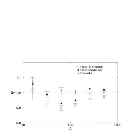
FIG. 1.: $\psi(L)=\sqrt{\frac{12\nu}{DL}}W(L)$ as a function of the size $L$ where $W(L)$ stands for the steady state roughness computed using the standard real space discretization Eq.(3), the modified real space discretization Eq.(4), and the Pseudo-spectral discretization given in Eq. (20) and Eq.(21) for a one-dimensional KPZ equation. The dotted line corresponds to the exact continuum value given by Eq. (47) ($\nu/D=1$). Units are arbitrary.

FIG. 2.: Temporal behavior of $g_{2}(t)$ for a KPZ growth on one dimensional substrate of size $L=256$. The temporal axis $t$ is written in terms of numbers of Euler time steps, here taken to be $10^{-3}$.

FIG. 3.: Temporal behavior of functions $g_{2}(t)$, $g_{2}^{(2)}(t)$ and $R_{2}^{(2)}(t)$ (see text) for a KPZ growth on one dimensional substrate of size $L=256$. The temporal axis $t$ is written in terms of numbers of Euler time steps $10^{-3}$.

FIG. 4.: The coupling parameter $\nu_{s}$ for various coarse-graining levels $b=2^{l}$ and for increasing lattice sizes $2048$, $4096$ and $8192$ in the case of a numerically generated KPZ equation. The input value is $\nu=1$. Error bars are of the order of the symbol sizes.

FIG. 5.: The coupling parameter $\lambda_{s}$ for various $b$ and increasing lattice sizes $2048$, $4096$ and $8192$ in the case of a numerically generated KPZ equation. The input value is $\lambda=3$.

FIG. 6.: The coupling parameter $D_{s}$ for various $b$ and for increasing lattice sizes $2048$, $4096$ and $8192$ in the case of a numerically generated KPZ equation. The input value is $D=1$.

FIG. 7.: The ratio $R\equiv\nu_{s}/D_{s}$ for the SS1 growth model.

FIG. 8.: The coupling parameter $\lambda_{s}$ for the SS1 growth model.

FIG. 9.: The coupling parameter $c_{s}$ for the SS1 growth model.

REFERENCES

- [1] A.S. Weigend and N.A. Gershenfeld, Time Series Prediction, Addison Wesley, (1994).
- [2] J. Krug, Adv. Phys. 46, 139 (1997)
- [3] A.L. Barabasi, H. E. Stanley, Fractal Concepts in Surface Growth (Cambridge University Press, Cambridge 1995)
- [4] T. Halpin-Haley and Y. C. Zhang, Phys. Rep. 254, 215 (1995)
- [5] M. Marsili, A. Maritan, F. Toigo and J. R. Banavar, Rev. Mod. Phys. 68, 963 (1996)
- [6] P. Meakin, Phys. Rep. 235, 131 (1993).
- [7] M. Kardar, G. Parisi and Y. C. Zhang, Phys. Rev. Lett. 56, 889 (1986).
- [8] H. Risken, The Fokker-Planck Equation, Springer-Verlag, Berlin, (1989).
- [9] S. F. Edward and D. R. Wilkinson, Proc. R. Soc. London A 381, 17 (1982).
- [10] C. Lam and F.G. Shin, Phys.Rev. E 58 ,5592 (1998).
- [11] C. Lam and F.G. Shin, Phys.Rev. E 57 ,6506 (1998).
- [12] A. Giacometti and M. Rossi, Phys.Rev. E 62, 1716 (2000).
- [13] A. Giacometti, A. Maritan, F. Toigo and J. R. Banavar, J. Stat. Phys. 79, 649 (1995); ibidem 82, 1669 (1996).
- [14] C.Canuto, M.Y. Hussaini, A. Quarteroni and T.A. Zang, ”Spectral Methods in Fluid Dynamics.” Springer-Verlag, Berlin (1988).
- [15] S. Zaleski, Physica D 34, 427 (1989)
- [16] F. Hayot, C. Jayaprakash, and Ch. Josserand Phys. Rev. E 47, 911 (1993).
- [17] After this work has been completed, we became aware that R.Toral has independently proposed a spectral approximation of the KPZ equation (private communication).
- [18] C. Lam and L.M. Sander, Phys.Rev. Lett. 71 , 561, (1993).
- [19] R.Mannella, Computer experiments in non-linear stochastic physics, in: Noise in nonlinear dynamical systems, vol. 3, ed. by F. Moss, P.V.E. McClintock, Cambridge University Press, Cambridge, (1989).
- [20] W. Press, S. A. Teukolsky, and W. T. Vetterling, Numerical Recipes (Cambridge University Press 1992)
- [21] J. Krug, P. Meakin and T. Halpin-Healy, Phys. Rev. A 45, 638 (1992).
- [22] P. Meakin, P. Ramanlal, L. M. Sander, and R. C. Ball, Phys. Rev. A 34, 5091 (1986).
- [23] B. M. Boghosian, C. C. Chow, and T. Hwa, Phys. Rev. Lett. 83 5262 (1999).