Critical Phenomena and Renormalization-Group Theory

Abstract

We review results concerning the critical behavior of spin systems at equilibrium. We consider the Ising and the general O($N$)-symmetric universality classes, including the $N\rightarrow 0$ limit that describes the critical behavior of self-avoiding walks. For each of them, we review the estimates of the critical exponents, of the equation of state, of several amplitude ratios, and of the two-point function of the order parameter. We report results in three and two dimensions. We discuss the crossover phenomena that are observed in this class of systems. In particular, we review the field-theoretical and numerical studies of systems with medium-range interactions.

Moreover, we consider several examples of magnetic and structural phase transitions, which are described by more complex Landau-Ginzburg-Wilson Hamiltonians, such as $N$-component systems with cubic anisotropy, O($N$)-symmetric systems in the presence of quenched disorder, frustrated spin systems with noncollinear or canted order, and finally, a class of systems described by the tetragonal Landau-Ginzburg-Wilson Hamiltonian with three quartic couplings. The results for the tetragonal Hamiltonian are original, in particular we present the six-loop perturbative series for the $\beta$-functions. Finally, we consider a Hamiltonian with symmetry O$(n_{1})\oplus$O$(n_{2})$ that is relevant for the description of multicritical phenomena.

Plan of the review

The main issue of this review is the critical behavior of spin systems at equilibrium.

In Sec. 1 we introduce the notations and the basic renormalization-group results for the critical exponents, the equation of state, and the two-point function of the order parameter, which are used throughout the paper.

In Sec. 2 we outline the most important methods that are used in the study of equilibrium spin systems: high-temperature expansions, Monte Carlo methods, and field-theoretical methods. It is not a comprehensive review of these techniques; the purpose is to present the most efficient methods and to discuss their possible sources of error.

In the following sections we focus on specific systems and universality classes. Sec. 3 is dedicated to the Ising universality class in three and two dimensions. Secs. 4 and 5 consider the three-dimensional $XY$ and Heisenberg universality classes respectively. In Sec. 6 we discuss the three-dimensional O($N$) universality classes with $N\geq 4$, with special emphasis on the physically relevant cases $N=4$ and $N=5$. Secs. 7 and 8 are devoted to the special critical behaviors of the two-dimensional models with continuous O($N$) symmetry, i.e. the Kosterlitz-Thouless transition, which occurs in the $XY$ model, and the peculiar exponential behavior characterizing the zero-temperature critical limit of the O($N$) vector model with $N\geq 3$. Finally, in Sec. 9 we discuss the limit $N\to 0$ that describes the asymptotic properties of self-avoiding walks and of polymers in dilute solutions and in the good-solvent regime. For each of these models, we review the estimates of the critical exponents, of the equation of state, of several universal amplitude ratios, and of the two-point function of the order parameter.

In Sec. 10 we discuss the crossover phenomena that are observed in this class of systems. In particular, we review the field-theoretic and numerical studies of systems with medium-range interactions.

In Sec. 11 we consider several examples of magnetic and structural phase transitions, which are described by more complex Landau-Ginzburg-Wilson Hamiltonians. We present field-theoretical results and we compare them with other theoretical and experimental estimates. In Sec. 11.3 we discuss $N$-component systems with cubic anisotropy, and in particular the stability of the O$(N)$-symmetric fixed point in the presence of cubic perturbations. In Sec. 11.4 we consider O($N$)-symmetric systems in the presence of quenched disorder, focusing on the randomly dilute Ising model that shows a different type of critical behavior. In Sec. 11.5 we discuss the critical behavior of frustrated spin systems with noncollinear or canted order. In Sec. 11.6 we discuss a class of systems described by the tetragonal Landau-Ginzburg-Wilson Hamiltonian with three quartic couplings. This section contains original results, in particular the six-loop perturbative series of the $\beta$-functions. Finally, in Sec. 11.7 we consider a Hamiltonian with symmetry O$(n_{1})\oplus$O$(n_{2})$, which is relevant for the description of multicritical phenomena.

Acknowledgements

We thank Tomeu Allés, Pasquale Calabrese, Massimo Campostrini, Sergio Caracciolo, José Carmona, Michele Caselle, Serena Causo, Alessio Celi, Robert Edwards, Martin Hasenbusch, Gustavo Mana, Victor Martín-Mayor, Tereza Mendes, Andrea Montanari, Paolo Rossi, Alan Sokal, for collaborating with us on some of the issues considered in this review.

1 The theory of critical phenomena

1.1 Introduction

The theory of critical phenomena has quite a long history. In the XIX century Andrews [47] discovered a peculiar point in the $P-T$ plane of carbon dioxide, where the properties of the liquid and of the vapor become indistinguishable and the system shows critical opalescence: It was the first observation of a critical point. Thirty years later, Pierre Curie [312] discovered the ferromagnetic transition in iron and realized the similarities of the two phenomena. However, a quantitative theory was still to come. Landau [683] was the first one proposing a general framework that provided a unified explanation of these phenomena. His model, which corresponds to the mean-field approximation, gave a good qualitative description of the transitions in fluids and magnets. However, Onsager’s solution [863] of the two-dimensional Ising model [561] and Guggenheim’s results on the coexistence curve of simple fluids [479] showed that Landau’s model is not quantitatively correct. In the early 60’s the modern notations were introduced by Fisher [400]. Several scaling relations among critical exponents were derived [375, 1113, 454], and a scaling form for the equation of state was proposed [1115, 346, 887]. A more general framework was introduced by Kadanoff [599]. However, a satisfactory understanding was reached only when the scaling ideas were reconsidered in the general renormalization-group (RG) framework by Wilson [1122, 1121, 1126]. Within the new framework, it was possible to explain the critical behavior of most of the systems and their universal features; for instance, why fluids and uniaxial antiferromagnets behave quantitatively in an identical way at the critical point.

Since then, critical phenomena have been the object of extensive studies and many new ideas have been developed in order to understand the critical behavior of increasingly complex systems. Moreover, the concepts that first appeared in condensed-matter physics have been applied to different areas of physics, such as high-energy physics, and even outside, e.g., to computer science, biology, economics, and social sciences.

In high-energy physics, the RG theory of critical phenomena provides the natural framework for defining quantum field theories at a nonperturbative level, i.e., beyond perturbation theory (see, e.g., Ref. [1152]). For example, the Euclidean lattice formulation of gauge theories proposed by Wilson [1123, 1124] provides a nonperturbative definition of quantum chromodynamics (QCD), the theory that is supposed to describe the strong interactions in subnuclear physics. QCD is obtained as the critical zero-temperature (zero-bare-coupling) limit of appropriate four-dimensional lattice models and may therefore be considered as a particular four-dimensional universality class, characterized by a peculiar exponential critical behavior (see, e.g., Refs. [308, 798, 1152, 570]). Wilson’s formulation represented a breakthrough in the study of QCD, because it lends itself to nonperturbative computations using statistical-mechanics techniques, for instance by means of Monte Carlo simulations (see, e.g., Ref. [309]).

The prototype of models with a continuous phase transition is the celebrated Ising model [561]. It is defined on a regular lattice with Hamiltonian

$${\cal H}=-J\sum_{\langle ij\rangle}s_{i}s_{j}-H\sum_{i}s_{i},$$ (1.1)

where $s_{i}=\pm 1$, and the first sum is extended over all nearest-neighbor pairs $\langle ij\rangle$. The partition function is defined by

$$Z=\sum_{\{s_{i}\}}e^{-{\cal H}/T}.$$ (1.2)

The Ising model provides a simplified description of a uniaxial magnet in which the spins align along a specific direction. The phase diagram of this system is well known, see Fig. 1.

Figure 1: The phase diagram of a magnetic system (left) and of a simple fluid (right).

For zero magnetic field, there is a paramagnetic phase for $T>T_{c}$ and a ferromagnetic phase for $T<T_{c}$, separated by a critical point at $T=T_{c}$. Near the critical point long-range correlations develop, and the large-scale behavior of the system can be studied using the RG theory.

The Ising model can easily be mapped into a lattice gas. Consider the Hamiltonian

$${\cal H}=-4J\sum_{\langle ij\rangle}\rho_{i}\rho_{j}-\,\mu\sum_{i}\rho_{i},$$ (1.3)

where $\rho_{i}=0,1$ depending if the site is empty or occupied, and $\mu$ is the chemical potential. If we define $s_{i}=2\rho_{i}-1$, we reobtain the Ising-model Hamiltonian with $H=2qJ+\mu/2$, where $q$ is the coordination number of the lattice. Thus, for $\mu=-4qJ$, there is an equivalent transition separating the gas phase for $T>T_{c}$ from a liquid phase for $T<T_{c}$.

Table 1: Relation between fluid and magnetic quantities. Here $\cal F$ and ${\cal A}$ are respectively the Gibbs and the Helmholtz free energy, $C_{P}$ and $C_{V}$ the isobaric and isochoric specific heats, $C_{M}$ and $C_{H}$ the specific heats at fixed magnetization and magnetic field, $\kappa_{T}$ the isothermic compressibility, and $\chi$ the magnetic susceptibility. $\rho_{c}$ and $\mu_{c}$ are the values of the density and of the chemical potential at the critical point.

FLUID	MAGNET
density: $\rho-\rho_{c}$	magnetization $M$
chemical potential: $\mu-\mu_{c}$	magnetic field $H$
$C_{P}=-T\displaystyle\left({\partial^{2}{\cal F}\over\partial T^{2}}\right)_{P}$	$C_{H}=-T\displaystyle\left({\partial^{2}{\cal F}\over\partial T^{2}}\right)_{H}$
$C_{V}=-T\displaystyle\left({\partial^{2}{\cal A}\over\partial T^{2}}\right)_{V}$	$C_{M}=-T\displaystyle\left({\partial^{2}{\cal A}\over\partial T^{2}}\right)_{M}$
${\kappa}_{T}=\displaystyle{1\over\rho}\left({\partial\rho\over\partial P}\right)_{T}=-{1\over V}\displaystyle\left({\partial^{2}{\cal F}\over\partial P^{2}}\right)_{T}$	$\chi=\displaystyle\left({\partial M\over\partial H}\right)_{T}=-\left({\partial^{2}{\cal F}\over\partial H^{2}}\right)_{T}$

The lattice gas is a crude approximation of a real fluid. Nonetheless, the universality of the behavior around a continuous phase-transition point implies that certain quantities, e.g., critical exponents, some amplitude ratios, scaling functions, and so on, are identical in a real fluid and in a lattice gas, and hence in the Ising model. Thus, the study of the Ising model provides exact predictions for the critical behavior of real fluids, and in general for all transitions belonging to the Ising universality class, whose essential features are a scalar order parameter and effective short-range interactions.

In the following, we will use a magnetic “language.” In Table 1 we write down the correspondences between fluid and magnetic quantities. The quantity that corresponds to the magnetic field is the chemical potential. However, such a quantity is not easily accessible experimentally, and thus one uses the pressure as second thermodynamic variable. The phase diagram of a real fluid is shown in Fig. 1 (right). The low-temperature line (in boldface) appearing in the magnetic phase diagram corresponds to the liquid-gas transition line between the triple and the critical point. Of course, this description is only valid in a neighborhood of the critical point. In magnetic systems there is a symmetry $M\to-M$, $H\to-H$ that is absent in fluids. As a consequence, although the leading critical behavior is identical, fluids show subleading corrections that are not present in magnets.

The generalization of the Ising model to systems with an $N$-vector order parameter and O($N$) symmetry provides other physically interesting universality classes describing several critical phenomena in nature, such as some ferromagnetic transitions, the superfluid transition of ⁴He, the critical behavior of polymers, etc.

This review will mostly focus on the critical behavior of $N$-vector models at equilibrium. This issue has been amply reviewed in the literature, see, e.g., Refs. [405, 411, 266, 1152, 570, 883, 746, 659]. Other reviews can be found in the Domb-Green-Lebowitz book series. We will mainly discuss the recent developments. Other systems, described by more complex Landau-Ginzburg-Wilson Hamiltonians, will be considered in the last section.

1.2 The models and the basic thermodynamic quantities

In this review we mainly deal with systems whose critical behavior can be described by the Heisenberg Hamiltonian (in Sec. 11 we will consider some more general theories that can be studied with similar techniques). More precisely, we consider a regular lattice, $N$-vector unit spins defined at the sites of the lattice, and the Hamiltonian

$${\cal H}=-\beta\sum_{\langle ij\rangle}\vec{s}_{i}\cdot\vec{s}_{j}-\sum_{i}\vec{H}\cdot\vec{s}_{i},$$ (1.4)

where the summation is extended over all lattice nearest-neighbor pairs $\langle ij\rangle$, and $\beta$ is the inverse temperature. This model represents the natural generalization of the Ising model, which corresponds to the case $N=1$. One may also consider more general Hamiltonians of the form

$${\cal H}=-\beta\sum_{\langle ij\rangle}\vec{\phi}_{i}\cdot\vec{\phi}_{j}+\sum_{i}V(\phi_{i})-\sum_{i}\vec{H}\cdot\vec{\phi}_{i},$$ (1.5)

where $\vec{\phi}_{i}$ is an $N$-dimensional vector and $V(x)$ is a generic potential such that

$$\int_{-\infty}^{\infty}e^{bx^{2}-V(x)}<+\infty$$ (1.6)

for all real $b$. A particular case is the $\phi^{4}$ Hamiltonian

$${\cal H}=-\beta\sum_{\langle ij\rangle}\vec{\phi}_{i}\cdot\vec{\phi}_{j}+\sum_{i}\left[\lambda(\vec{\phi}_{i}^{\ 2}-1)^{2}+\phi_{i}^{2}\right]-\sum_{i}\vec{H}\cdot\vec{\phi}_{i},$$ (1.7)

which is the lattice discretization of the continuum theory

$${\cal H}=\int d^{d}x\Bigl{\{}{\textstyle\frac{1}{2}}\partial_{\mu}\vec{\varphi}(x)\cdot\partial_{\mu}\vec{\varphi}(x)+{\textstyle\frac{1}{2}}{r}\,\vec{\varphi}(x)\cdot\vec{\varphi}(x)+{\textstyle\frac{1}{4!}}u\left[\vec{\varphi}(x)\cdot\vec{\varphi}(x)\right]^{2}-\vec{H}\cdot\vec{\varphi}(x)\Bigr{\}},$$ (1.8)

where, in the case of a hypercubic lattice,

$$\varphi=\beta^{1/2}\phi,\qquad r={2-4\lambda\over\beta}-2d,\qquad u={4!\ \lambda\over\beta^{2}}.$$ (1.9)

The partition function is given by

$$Z(H,T)=\int\left[\prod_{i}d\mu(\vec{\phi}_{i})\right]\,e^{-{\cal H}},$$ (1.10)

where $d\mu(\vec{\phi})=d^{N}\!\phi$ when $\phi$ is an unconstrained vector and $d\mu(\vec{s})=d^{N}\!s\,\delta(s^{2}-1)$ for the Heisenberg Hamiltonian. We will only consider the classical case, i.e., our spins will always be classical fields and not quantum operators.

As usual, we introduce the Gibbs free-energy density

$${\cal F}(H,T)=-{1\over V}\log Z(H,T),$$ (1.11)

and the related Helmholtz free-energy density

$${\cal A}(M,T)=\vec{M}\cdot\vec{H}+{\cal F}(H,T),$$ (1.12)

where $V$ is the volume. Here $\vec{M}$ is the magnetization density defined by

$$\vec{M}=-\left({\partial{\cal F}\over\partial\vec{H}}\right)_{T}.$$ (1.13)

General arguments of thermal and mechanical stability imply $C_{P}\geq 0$, $C_{V}\geq 0$, and $\kappa_{T}\geq 0$, and also $C_{H}\geq 0$, $C_{M}\geq 0$, and $\chi\geq 0$. These results allow us to prove the convexity properties of the free energy, for instance using Hölder’s inequality [472]. The positivity of the specific heats at constant magnetic field and magnetization and of the susceptibility implies that the Gibbs free energy is concave in $T$ and $H$, and the Helmholtz free energy is concave in $T$ and convex in $M$.

We consider several thermodynamic quantities:

1. The magnetic susceptibility $\chi$:

   $$\chi=-{\partial^{2}{\cal F}\over\partial\vec{H}\cdot\partial\vec{H}}=\sum_{x}\left[\langle\vec{\phi}_{x}\cdot\vec{\phi}_{0}\rangle-\langle\vec{\phi}_{0}\rangle^{2}\right].$$ (1.14)

   For vector systems one may also define

   $$\chi^{ab}=-{\partial^{2}{\cal F}\over\partial H^{a}\partial H^{b}},$$ (1.15)

   and, if $H^{a}=H\delta^{a1}$, the transverse and longitudinal susceptibilities

   $$\chi_{L}=\chi^{11},\qquad\chi_{T}={1\over(N-1)}(\chi-\chi_{L}).$$ (1.16)

   Note that $\chi^{ab}=\delta^{ab}\chi_{T}$ for $a,b\not=1$, because of the residual $O(N-1)$ invariance.

2. The $2n$-point connected correlation function $\chi_{2n}$ at zero momentum:

   $$\chi_{2n}=-{\partial^{2n}{\cal F}\over(\partial\vec{H}\cdot\partial\vec{H})^{n}}.$$ (1.17)

   For the Ising model in the low-temperature phase one should also consider odd derivatives of the Gibbs free energy $\chi_{2n+1}$.

3. The specific heat at fixed magnetic field and at fixed magnetization:

   $$C_{H}=-T\left({\partial^{2}{\cal F}\over\partial T^{2}}\right)_{H},\qquad C_{M}=-T\left({\partial^{2}{\cal A}\over\partial T^{2}}\right)_{M}.$$ (1.18)

4. The two-point correlation function:

   $$G(x)=\langle\vec{\phi}_{x}\cdot\vec{\phi}_{0}\rangle-\langle\vec{\phi}_{0}\rangle^{2},$$ (1.19)

   whose zero-momentum component is the magnetic susceptibility, i.e. $\chi=\sum_{x}G(x)$. In the low-temperature phase, for vector models, one distinguishes transverse and longitudinal contributions. If $H^{a}=H\delta^{a1}$ we define

   $$G_{L}(x)=\langle{\phi}_{x}^{1}\,{\phi}_{0}^{1}\rangle-M^{2},\qquad G_{T}(x)=\langle{\phi}_{x}^{a}\,{\phi}_{0}^{a}\rangle,$$ (1.20)

   where $a\not=1$ is not summed over.

5. The exponential or true correlation length (inverse mass gap)

   $$\xi_{\rm gap}=-\lim\sup_{|x|\to\infty}{|x|\over\log G(x)}\;.$$ (1.21)

6. The second-moment correlation length

   $$\xi=\left[{1\over 2d}\,{\sum_{x}|x|^{2}G(x)\over\sum_{x}G(x)}\right]^{1/2}.$$ (1.22)

1.3 Critical indices and scaling relations

In three dimensions and for $H=0$, the Hamiltonian (1.5) displays a low-temperature magnetized phase separated from a paramagnetic phase by a critical point. The transition may be either first-order or continuous, depending on the potential $V(\phi)$. The continuous transitions are generically characterized by a nontrivial power-law critical behavior controlled by two relevant quantities, the temperature and the external field. Specific choices of the parameters may lead to multicritical transitions. For instance, tricritical transitions require the additional tuning of one parameter in the potential; in three dimensions they have mean-field exponents with logarithmic corrections. We shall not consider them here. The interested reader should consult Ref. [689].

In two dimensions a power-law critical behavior is observed only for $N<2$. For $N=2$ the systems show a Kosterlitz-Thouless transition [670] with a different scaling behavior. This is described in Sec. 7. For $N\geq 3$ there is no finite-temperature phase transition and correlations are finite for all temperatures $T\not=0$, diverging for $T\to 0$. These systems are discussed in Sec. 8. In this section we confine ourselves to the “standard” critical behavior characterized by power laws.

When the reduced temperature

$$t\equiv{T-T_{c}\over T_{c}}={\beta_{c}-\beta\over\beta}$$ (1.23)

goes to zero and the magnetic field vanishes, all quantities show power-law singularities. It is customary to consider three different trajectories in the $(t,H)$ plane.

• The high-temperature phase at zero field: $t>0$ and $H=0$. For $t\to 0$ we have

  $$T_{c}C_{H}\approx A^{+}\ t^{-\alpha},\\$$ (1.24)

  for the specific heat, and

  $$\chi\approx NC^{+}\ t^{-\gamma},\qquad \chi_{2n}\approx R_{n,N}C^{+}_{2n}\ t^{-\gamma_{2n}},$$ (1.25)

  $$\xi\approx f^{+}\ t^{-\nu},\qquad \xi_{\rm gap}\approx f^{+}_{\rm gap}\ t^{-\nu},$$ (1.26)

  where $R_{n,N}={N(N+2)\ldots(N+2n-2)/(2n-1)!!}$ (note that $R_{n,1}=1$). In this phase the magnetization vanishes.

• The coexistence curve: $t<0$ and $H=0$. In this case we should distinguish scalar systems ($N=1$) from vector systems $(N\geq 2)$. Indeed, on the coexistence line vector systems show Goldstone excitations and the two-point function at zero momentum diverges. Therefore, $\chi$, $\chi_{2n}$, $\xi$, and $\xi_{\rm gap}$ are infinite at the coexistence curve, i.e. for $|H|\to 0$ and any $t<0$. We define

  $$T_{c}C_{H} \approx A^{-}\ (-t)^{-\alpha^{\prime}},$$ (1.27)

  $$|M| \approx B(-t)^{\beta},$$ (1.28)

  and for a scalar theory

  $$\chi\approx C^{-}\ (-t)^{-\gamma^{\prime}},\qquad \chi_{n}\approx C^{-}_{n}\ (-t)^{-\gamma_{n}^{\prime}},$$ (1.29)

  $$\xi\approx f^{-}\ (-t)^{-\nu^{\prime}},\qquad \xi_{\rm gap}\approx f^{-}_{\rm gap}\ (-t)^{-\nu^{\prime}}.$$ (1.30)

  In the case of vector models, a transverse correlation length [383]

  $$\xi_{\rm T}\approx f^{-}_{\rm T}(-t)^{-\nu^{\prime}}$$ (1.31)

  is defined from the stiffness constant $\rho_{s}$ (see Eq. (1.136) below for the definition). In the case of the Ising model, another interesting quantity is the interface tension $\sigma$, which, for $t\to 0^{-}$, behaves as

  $$\sigma=\sigma_{0}(-t)^{\mu}.$$ (1.32)

• The critical isotherm $t=0$. For $|H|\to 0$ we have

  $$\vec{M}\approx B^{c}\vec{H}\ |H|^{(1-\delta)/\delta},\qquad\xi\approx f^{c}|H|^{-\nu_{c}},\qquad\xi_{\rm gap}\approx f^{c}_{\rm gap}|H|^{-\nu_{c}}.$$ (1.33)

  The scaling of the $n$-point connected correlation functions is easily obtained from that of $\vec{M}$ by taking derivatives with respect to $\vec{H}$. For instance, we have

  $$\chi\approx C^{c}|H|^{(1-\delta)/\delta},\qquad\chi_{L}\approx C_{L}^{c}|H|^{(1-\delta)/\delta},$$ (1.34)

  where

  $$C^{c}={B^{c}\over\delta}(1+N\delta-\delta),\qquad C_{L}^{c}={B^{c}\over\delta}.$$ (1.35)

Moreover, one introduces the exponent $\eta$ to describe the behavior of the two-point function at the critical point $T=T_{c}$, $H=0$, i.e.,

$$G(x)\sim{1\over|x|^{d-2+\eta}}\;.$$ (1.36)

The critical exponent $\eta$ measures the deviations from a purely Gaussian behavior.

The exponents that we have introduced are not independent. Indeed, RG predicts several relations among them. First, the exponents in the high-temperature phase and on the coexistence curve are identical, i.e.

$$\alpha=\alpha^{\prime},\qquad\nu=\nu^{\prime},\qquad\gamma=\gamma^{\prime},\qquad\gamma_{2n}=\gamma_{2n}^{\prime},$$ (1.37)

Second, the following relations hold:

$$\alpha+2\beta+\gamma=2,\qquad 2-\alpha=\beta(\delta+1),\qquad\beta\delta\nu_{c}=\nu,$$

$$\gamma=\nu(2-\eta),\qquad\gamma_{2n}=\gamma+2(n-1)\Delta_{\rm gap},$$ (1.38)

where $\Delta_{\rm gap}$ is the “gap” exponent, which controls the radius of the disk in the complex-temperature plane without zeroes, i.e. the gap, of the partition function (Yang-Lee theorem). Below the upper critical dimension, i.e. for $d<4$, also the following “hyperscaling” relations are supposed to be valid:

$$2-\alpha=d\nu,\qquad 2\Delta_{\rm gap}=d\nu+\gamma.$$ (1.39)

Moreover, the exponent $\mu$ related to the interface tension in the Ising model satisfies the hyperscaling relation [1114] $\mu=(d-1)\nu$. Using the scaling and hyperscaling relations, one also obtains

$$\delta={d+2-\eta\over d-2+\eta},\qquad\beta={\nu\over 2}\left(d-2+\eta\right).$$ (1.40)

For $d>4$ the hyperscaling relations do not hold, and the critical exponents assume the mean-field values:

$$\gamma=1,\quad\nu={1\over 2},\quad\eta=0,\quad\alpha=0,\quad\beta={1\over 2},\quad\delta=3,\quad\mu={3\over 2}.$$ (1.41)

In the following we only consider the case $d<4$ and thus we use the hyperscaling relations.

It is important to remark that the scaling behavior of the specific heat given above, cf. Eqs. (1.24) and (1.27), is correct only if $\alpha>0$. If $\alpha<0$ the analytic background cannot be neglected, and the critical behavior is

$$T_{c}C_{H}\approx A^{\pm}|t|^{-\alpha}+B$$ (1.42)

for $\alpha>-1$. The amplitudes $A^{\pm}$ are positive (resp. negative) for $\alpha>0$ (resp. $\alpha<0$), see, e.g., Ref. [227]. This fact is confirmed by the critical behavior of all known systems in the universality classes corresponding to $N$-vector models. Moreover, there are interesting cases, for instance the two-dimensional Ising model, in which the specific heat diverges logarithmically,

$$T_{c}C_{H}\approx-A^{\pm}\log|t|.$$ (1.43)

The critical behaviors reported in this section are valid asymptotically close to the critical point. Scaling corrections are controlled by a universal exponent $\omega$, which is related to the RG dimension of the leading irrelevant operator. For $H=0$, both in the high- and in the low-temperature phase, the scaling corrections are of order $|t|^{\Delta}$ with $\Delta=\omega\nu$, while on the critical isotherm they are of order $|H|^{\Delta_{c}}$ with $\Delta_{c}=\omega\nu_{c}$.

The critical exponents are universal in the sense that they have the same value for all systems belonging to a given universality class. The amplitudes instead are not universal and depend on the microscopic parameters, and therefore on the particular system considered. Nonetheless, RG predicts that some combinations are universal. Several universal amplitude ratios are reported in Table 2. Those involving the amplitudes of the susceptibilities and of the correlation lengths on the coexistence curve, and the amplitude of the interface tension are defined only for a scalar theory (Ising universality class).

Table 2: Definitions of several universal amplitude ratios. Those involving $C^{-}$, $C^{-}_{n}$, $f^{-}$, $f^{-}_{\rm gap}$, and $\sigma_{0}$ are defined only for $N=1$.

Universal Amplitude Ratios
$U_{0}\equiv A^{+}/A^{-}$	$U_{2}\equiv C^{+}/C^{-}$
$U_{4}\equiv C^{+}_{4}/C^{-}_{4}$	$R_{4}^{+}\equiv-C_{4}^{+}B^{2}/(C^{+})^{3}$
$R_{c}^{+}\equiv\alpha A^{+}C^{+}/B^{2}$	$R_{c}^{-}\equiv\alpha A^{-}C^{-}/B^{2}$
$R_{4}^{-}\equiv C_{4}^{-}B^{2}/(C^{-})^{3}$	$R_{\chi}\equiv C^{+}B^{\delta-1}/(B^{c})^{\delta}$
$v_{3}\equiv-C_{3}^{-}B/(C^{-})^{2}$	$v_{4}\equiv-C_{4}^{-}B^{2}/(C^{-})^{3}+3v_{3}^{2}$
$g_{4}^{+}\equiv-C_{4}^{+}/[(C^{+})^{2}(f^{+})^{d}]$	$w^{2}\equiv C^{-}/[B^{2}(f^{-})^{d}]$
$U_{\xi}\equiv f^{+}/f^{-}$	$U_{\xi_{\rm gap}}\equiv f^{+}_{\rm gap}/f^{-}_{\rm gap}$
$Q^{+}\equiv\alpha A^{+}(f^{+})^{d}$	$Q^{-}\equiv\alpha A^{-}(f^{-})^{d}$
$R^{+}_{\xi}\equiv(Q^{+})^{1/d}$	$Q^{+}_{\xi}\equiv f^{+}_{\rm gap}/f^{+}$
$Q^{-}_{\xi}\equiv f^{-}_{\rm gap}/f^{-}$	$Q^{c}_{\xi}\equiv f^{c}_{\rm gap}/f^{c}$
$Q_{c}\equiv B^{2}(f^{+})^{d}/C^{+}$	$Q_{2}\equiv(f^{c}/f^{+})^{2-\eta}C^{+}/C^{c}$
$R_{\sigma}\equiv\sigma_{0}(f^{-})^{d-1}$	$R_{\sigma}^{+}\equiv\sigma_{0}(f^{+})^{d-1}$
$P_{m}\equiv{T_{p}^{\beta}B/B^{c}}$	$R_{p}\equiv{C^{+}/C_{p}}$

We also consider another trajectory in the $(T,H)$ plane, the crossover or pseudocritical line $t_{\rm max}(H)$, which is defined as the reduced temperature for which the longitudinal magnetic susceptibility $\chi_{L}(t,H)$ has a maximum at $|H|$ fixed. RG predicts

$$t_{\rm max}(H)=T_{p}|H|^{1/(\gamma+\beta)},\qquad\qquad\chi_{L}(t_{\rm max},H)=C_{p}t_{\rm max}^{-\gamma}.$$ (1.44)

Some related universal amplitude ratios are defined in Table 2.

Finally, we mention the relation between ferromagnetic and antiferromagnetic models on bipartite lattices, such as simple cubic and bcc lattices. In an antiferromagnetic model the relevant critical quantities are the staggered ones. For instance, on a cubic lattice the staggered susceptibility is given by

$$\chi_{\rm stagg}=\sum_{x}(-1)^{p(x)}\langle\sigma_{0}\sigma_{x}\rangle,$$ (1.45)

where $p(x)={\rm mod}\ (x_{1}+\ldots+x_{d},2)$ is the parity of $x$. One may easily prove that $\chi_{\rm stagg}=\chi_{\rm ferro}$, where $\chi_{\rm ferro}$ is the ordinary susceptibility in the ferromagnetic model. The critical behavior of the staggered quantities is identical to the critical behavior of the zero-momentum quantities in the ferromagnetic model. The critical behavior of the usual thermodynamic quantities in antiferromagnets is different, although still related to that of the ferromagnetic model. For instance, the susceptibility behaves as [399]

$$\chi\approx c_{0}+c_{1}t+\ldots+b_{0}|t|^{1-\alpha}+\ldots$$ (1.46)

Higher-order moments of the two-point function, i.e. $\sum_{x}|x|^{n}G(x)$, show a similar behavior [243].

1.4 Rigorous results for $N=1$

Several rigorous results have been obtained for spin systems with $N=1$ and $N\rightarrow 0$ (as we shall see, in the limit $N\rightarrow 0$ spin models can be mapped into walk models, see Sec. 9). We report here only the most relevant ones for $N=1$ and refer the reader to Refs. [83, 388, 749] for a detailed presentation of the subject. Most of the results deal with the general ferromagnetic Hamiltonian

$${\cal H}=-\sum_{i<j}K_{ij}\phi_{i}\phi_{j}-\sum_{i}h_{i}\phi_{i},$$ (1.47)

where $K_{ij}$, $h_{i}$ are arbitrary positive numbers, and the first sum is extended over all lattice pairs. The partition function is given by

$$Z=\int\prod_{i}\ \left[d\phi_{i}\;F(\phi_{i})\right]\;e^{-{\cal H}},$$ (1.48)

where $F(x)$ is an even function satisfying

$$\int_{-\infty}^{\infty}dx\,F(x)\,e^{bx^{2}}<+\infty,$$ (1.49)

for all real $b$. For this class of Hamiltonians the following results have been obtained:

• Fisher [404] proved the inequality: $\gamma\leq(2-\eta)\nu$.

• Sokal [1019] proved that $\chi\leq{\rm const}(1+\xi^{2})$ for $T>T_{c}$, implying $\gamma\leq 2\nu$. If we assume the scaling relation $\gamma=(2-\eta)\nu$, then $\eta\nu\geq 0$, and $\eta\geq 0$ since $\nu>0$.

• The following Buckingham-Gunton inequalities have been proved [203, 404]:

  $$2-\eta\leq{d\gamma^{\prime}\over 2\beta+\gamma^{\prime}}\leq\;{d\gamma^{\prime}\over 2-\alpha^{\prime}},\qquad 2-\eta\leq d{\delta-1\over\delta+1}.$$ (1.50)

• Sokal [1018] proved that $d\nu^{\prime}\geq\gamma^{\prime}+2\beta\geq 2-\alpha^{\prime}$.

Moreover, for the $\phi^{4}$ theory it has been shown that [462, 81] $\gamma\geq 1$, from which one may derive $\nu\geq 1/2$ using $\gamma\leq 2\nu$.

Several additional results have been proved for $d>4$, showing that the exponents have mean-field values. In particular, Aizenman [27] proved that $\gamma=1$, and then [28] that $\beta=1/2$ and $\delta=3$ for all $d\geq 5$. Moreover, for the zero-momentum four-point coupling $g_{4}$ defined by $g_{4}\equiv-\chi_{4}/(\chi^{2}\xi^{d})$, the inequality [27]

$$0\leq g_{4}\leq{{\rm const}\over\xi^{d-4}}\to 0$$ (1.51)

holds, implying the absence of scattering (triviality) above four dimensions. For $d=4$ the RG results [687, 1107, 175]

$$\chi(t)\sim t^{-1}|\log t|^{1/3},\qquad\xi_{\rm gap}(t)\sim t^{-1/2}|\log t|^{1/6},\qquad g_{4}\sim{1\over n_{0}+|\log t|},$$ (1.52)

where $n_{0}$ is a positive constant, have been proved for the weakly coupled $\phi^{4}$ theory [506, 507].

1.5 Scaling behavior of the free energy and of the equation of state

1.5.1 Renormalization-group scaling

According to RG, the Gibbs free energy obeys a general scaling law. Indeed, we can write it in terms of the nonlinear scaling fields associated with the RG eigenoperators at the fixed point. If $u_{i}$ are the scaling fields—they are analytic functions of $t$, $H$, and of any parameter appearing in the Hamiltonian—we have

$${\cal F}(H,t)={\cal F}_{\rm reg}(H,t)+{\cal F}_{\rm sing}(u_{1},u_{2},\ldots,u_{n},\ldots),$$ (1.53)

where ${\cal F}_{\rm reg}(H,t)$ is an analytic (also at the critical point) function of $H$ and $t$ which is usually called background or bulk contribution. The function ${\cal F}_{\rm sing}$ obeys a scaling law of the form [1105]:

$${\cal F}_{\rm sing}(u_{1},u_{2},\ldots,u_{n},\ldots)=b^{-d}{\cal F}_{\rm sing}(b^{y_{1}}u_{1},b^{y_{2}}u_{2},\ldots,b^{y_{n}}u_{n},\ldots),$$ (1.54)

where $b$ is any positive number and $y_{n}$ are the RG dimensions of the scaling fields. In the models that we consider, there are two relevant fields with $y_{i}>0$, and an infinite set of irrelevant fields with $y_{i}<0$. The relevant scaling fields are associated with the temperature and the magnetic field. We assume that they correspond to $u_{1}$ and $u_{2}$. Then $u_{1}\sim t$ and $u_{2}\sim|H|$ for $t,|H|\to 0$. If we fix $b$ by requiring $b^{y_{1}}|u_{1}|=1$ in Eq. (1.54), we obtain

$${\cal F}_{\rm sing}(u_{1},u_{2},\ldots,u_{n},\ldots)=|u_{1}|^{d/y_{1}}{\cal F}_{\rm sing}({\rm sign}\,u_{1},u_{2}|u_{1}|^{-y_{2}/y_{1}},\ldots,u_{n}|u_{1}|^{-y_{n}/y_{1}},\ldots).$$ (1.55)

For $n>2$, $y_{i}<0$, so that $u_{n}|u_{1}|^{-y_{n}/y_{1}}\to 0$ for $t\to 0$. Thus, provided that ${\cal F}_{\rm sing}$ is finite and nonvanishing in this limit, we can rewrite

$${\cal F}_{\rm sing}(u_{1},u_{2},\ldots,u_{n},\ldots)\approx|t|^{d/y_{1}}{\cal F}_{\rm sing}({\rm sign}\,t,|H||t|^{-y_{2}/y_{1}},0,0,\dots).$$ (1.56)

Using Eqs. (1.53) and (1.56), we obtain all scaling and hyperscaling relations provided that we identify

$$y_{1}={1\over\nu},\qquad\qquad y_{2}={\beta+\gamma\over\nu}.$$ (1.57)

Note that the scaling part of the free energy is expressed in terms of two different functions, depending on the sign of $t$. However, since the free energy is analytic along the critical isotherm for $H\not=0$, the two functions are analytically related.

It is possible to avoid the introduction of two different functions by fixing $b$ so that $b^{y_{2}}|u_{2}|=1$. This allows us to write, for $t\to 0$ and $|H|\to 0$,

$${\cal F}_{\rm sing}(u_{1},u_{2},\ldots,u_{n},\ldots)\approx|H|^{d/y_{2}}{\cal F}_{\rm sing}(t|H|^{y_{1}/y_{2}},1,0,0,\ldots),$$ (1.58)

where we have used the fact that the free energy does not depend on the direction of $\vec{H}$.

In conclusion, for $|t|\to 0$, $|H|\to 0$, $t|H|^{-1/(\beta+\gamma)}$ fixed, we have

$${\cal F}(H,t)-{\cal F}_{\rm reg}(H,t)\approx|t|^{d\nu}\widehat{\cal F}_{1,\pm}(H|t|^{-\beta-\gamma})=|H|^{d\nu/(\beta+\gamma)}\widehat{\cal F}_{2}(t|H|^{-1/(\beta+\gamma)}),$$ (1.59)

where $\widehat{\cal F}_{1,\pm}$ apply for $\pm t>0$ respectively. Note that $d\nu=2-\alpha$ and $d\nu/(\beta+\gamma)=1+1/\delta$. The functions $\widehat{\cal F}_{1,\pm}$ and $\widehat{\cal F}_{2}$ are universal apart from trivial rescalings. Eq. (1.59) is valid in the critical limit. Two types of corrections are expected: analytic corrections due to the fact that $u_{1}$ and $u_{2}$ are analytic functions of $t$ and $|H|$, and nonanalytic ones due to the irrelevant operators. The leading nonanalytic correction is of order $|u_{1}|^{-y_{3}/y_{1}}\sim t^{\Delta}$, or $|u_{2}|^{-y_{3}/y_{2}}\sim|H|^{\Delta_{c}}$, where we have identified $y_{3}=-\omega$, $\Delta=\omega\nu$, $\Delta_{c}=\omega\nu_{c}$.

The Helmholtz free energy obeys similar laws. In the critical limit, for $t\to 0$, $|M|\to 0$, and $t|M|^{-1/\beta}$ fixed, it can be written as

$$\Delta{\cal A}={\cal A}(M,t)-{\cal A}_{\rm reg}(M,t)\approx|t|^{d\nu}\widehat{\cal A}_{1,\pm}(|M||t|^{-\beta})=|M|^{\delta+1}\widehat{\cal A}_{2}(t|M|^{-1/\beta}),$$ (1.60)

where ${\cal A}_{\rm reg}(M,t)$ is a regular background contribution and $\widehat{\cal A}_{1,\pm}$ apply for $\pm t>0$ respectively. The functions $\widehat{\cal A}_{1,\pm}$ and $\widehat{\cal A}_{2}$ are universal apart from trivial rescalings. The equation of state is then given by

$$\vec{H}={\partial{\cal A}\over\partial\vec{M}}.$$ (1.61)

1.5.2 Normalized free energy and related quantities

In this section we define some universal functions related to $\widehat{\cal A}_{1,+}$ and $\widehat{\cal A}_{2}$. The function $\widehat{\cal A}_{1,-}$ for Ising systems will be discussed in Sec. 1.5.4.

The function $\widehat{\cal A}_{1,+}(|M|t^{-\beta})$ may be written in terms of a universal function $A_{1}(z)$ normalized in the high-temperature phase. The analyticity of the free energy outside the critical point and the coexistence curve (Griffiths’ analyticity) implies that $\widehat{\cal A}_{1,+}(|M|t^{-\beta})$ has a regular expansion in powers of $|M|^{2}t^{-2\beta}$. We introduce a new variable

$$z\equiv b_{1}|M|t^{-\beta},$$ (1.62)

and write

$$\widehat{\cal A}_{1,+}(|M|t^{-\beta})=a_{10}+a_{11}A_{1}(z),$$ (1.63)

where the constants are fixed by requiring that

$$A_{1}(z)={z^{2}\over 2}+{z^{4}\over 4!}+O(z^{6}).$$ (1.64)

The constants $a_{10}$, $a_{11}$, and $b_{1}$ can be expressed in terms of amplitudes that have been already introduced, i.e.,

$$a_{10}=-{A^{+}\over(2-\alpha)(1-\alpha)},\qquad a_{11}=-{(C^{+})^{2}\over C^{+}_{4}},\qquad b_{1}=\left[-{C^{+}_{4}\over(C^{+})^{3}}\right]^{1/2}.$$ (1.65)

They are not universal since they are normalization factors. On the other hand, the ratio $a_{11}/a_{10}$ and the function $A_{1}(z)$ are universal. It is worth mentioning that the ratio $a_{11}/a_{10}$ can be computed from the function $A_{1}(z)$ alone. Indeed, given the function $A_{1}(z)$, there is a unique constant $c$ such that $t^{2-\alpha}(c+A_{1}(z))$ is analytic on the critical isotherm. Such a constant is the ratio $a_{10}/a_{11}$.

The function $\widehat{\cal A}_{2}(t|M|^{-1/\beta})$ is usually normalized imposing two conditions, respectively at the coexistence curve and on the critical isotherm. We introduce

$$x\equiv B^{1/\beta}\,t|M|^{-1/\beta},$$ (1.66)

where $B$ is the amplitude of the magnetization, so that $x=-1$ corresponds to the coexistence curve. Then, we define

$$\widehat{\cal A}_{2}(t|M|^{-1/\beta})=a_{20}A_{2}(x),$$ (1.67)

requiring $A_{2}(0)=1$. This fixes the constant $a_{20}$:

$$a_{20}={(B^{c})^{-\delta}\over\delta+1}.$$ (1.68)

Again, $a_{20}$ is nonuniversal while $A_{2}(x)$ is universal.

The functions $A_{1}(z)$ and $A_{2}(x)$ are related:

$$A_{1}(z)=-{a_{10}\over a_{11}}+B^{\delta+1}{a_{20}\over a_{11}}\ x^{-d\nu}\ A_{2}(x).$$ (1.69)

The scaling equation of state can be written as

$$\vec{H}=a_{11}b_{1}{\vec{M}\over|M|}t^{\beta\delta}F(z)=(B^{c})^{-\delta}\vec{M}|M|^{\delta-1}f(x),$$ (1.70)

and

$$F(z)\equiv{A_{1}^{\prime}}(z)\qquad\qquad f(x)\equiv A_{2}(x)-{x\over d\nu}{A_{2}^{\prime}}(x)$$ (1.71)

Note that $f(0)=1$, since $A_{2}(0)=1$, and $f(-1)=0$ since $x=-1$ corresponds to the coexistence curve.

By solving Eq. (1.71) with the appropriate boundary conditions, it is possible to reobtain the free energy. This is trivial in the case of $A_{1}(z)$. In the case of $A_{2}(x)$ we have

$$A_{2}(x)=f(x)+{xf^{\prime}(0)\over 1-\alpha}-|x|^{2-\alpha}\int^{x}_{0}dy\ |y|^{\alpha-2}\left[f^{\prime}(y)-f^{\prime}(0)\right]$$ (1.72)

for $\alpha>0$, see, e.g., Ref. [107]. For $-1<\alpha<0$ one needs to perform an additional subtraction within the integral [107].

It is useful to define universal functions starting from the Gibbs free energy, cf. Eq. (1.59). We introduce a variable

$$y\equiv\left({B\over B^{c}}\right)^{1/\beta}t|H|^{-1/(\beta+\gamma)},$$ (1.73)

and define

$$\widehat{\cal F}_{2}(t|H|^{-1/(\beta+\gamma)})=-{\delta B^{c}\over{\delta+1}}\,G(y),$$ (1.74)

so that $G(0)=1$. The equation of state can now be written as

$$\vec{M}=B^{c}\vec{H}\,|H|^{(1-\delta)/\delta}E(y),\qquad E(y)=G(y)-{y\over d\nu}{\partial G\over\partial y}\;.$$ (1.75)

Clearly, $E(y)$ and $f(x)$ are related:

$$E(y)=f(x)^{-1/\delta},\qquad y=xf(x)^{-1/(\beta+\gamma)}.$$ (1.76)

Finally, we introduce a scaling function associated with the longitudinal susceptibility, by writing

$$\chi_{L}=B^{c}|H|^{1/\delta-1}D(y),$$ (1.77)

where

$$D(y)={1\over\delta}\left[E(y)-{y\over\beta}E^{\prime}(y)\right]={\beta f(x)^{1-1/\delta}\over\beta\delta f(x)-xf^{\prime}(x)}.$$ (1.78)

The function $D(y)$ has a maximum at $y=y_{\rm max}$ corresponding to the crossover line defined in Sec. 1.3. We can relate $y_{\rm max}$ and $D(y_{\rm max})$ to the amplitude ratios $P_{m}$ and $R_{p}$ defined along the crossover line, see Table 2,

$$y_{\rm max}=\left(P_{m}\right)^{1/\beta},\qquad D(y_{\rm max})=R_{p}^{-1}P_{m}^{1-\delta}R_{\chi}.$$ (1.79)

1.5.3 Expansion of the equation of state

The free energy is analytic in the $(T,H)$ plane outside the critical point and the coexistence curve. As a consequence, the functions $A_{1}(z)$ and $F(z)$ have a regular expansion in powers of $z$, with the appropriate symmetry under $z\to-z$. The expansion of $F(z)$ can be written as

$$F(z)=\,z+{\textstyle\frac{1}{6}}z^{3}+\sum_{n=3}{r_{2n}\over(2n-1)!}z^{2n-1}.$$ (1.80)

The constants $r_{2n}$ can be computed in terms of the $2n$-point functions $\chi_{2n}$ for $H=0$ and $t\to 0^{+}$. Explicitly

$$r_{6}=10-{C^{+}_{6}C^{+}\over(C^{+}_{4})^{2}},$$

$$r_{8}=280-56{C^{+}_{6}C^{+}\over(C^{+}_{4})^{2}}+{C^{+}_{8}(C^{+})^{2}\over(C^{+}_{4})^{3}},$$

$$r_{10}=15400-4620{C^{+}_{6}(C^{+})\over(C^{+}_{4})^{2}}+126{(C^{+}_{6})^{2}(C^{+})^{2}\over(C^{+}_{4})^{4}}+120{C^{+}_{8}(C^{+})^{2}\over(C^{+}_{4})^{3}}-{C^{+}_{10}(C^{+})^{3}\over(C^{+}_{4})^{4}},$$ (1.81)

etc. The coefficients $r_{2n}$ are related to the $2n$-point renormalized coupling constants $g_{2n}^{+}\equiv\,r_{2n}\,(g_{4}^{+})^{n-1}$. Griffiths’ analyticity implies that ${\cal A}(M,t)$ has also a regular expansion in powers of $t$ for $|M|$ fixed. As a consequence, $F(z)$ has the following large-$z$ expansion

$$F(z)=z^{\delta}\sum_{k=0}F^{\infty}_{k}z^{-k/\beta}.$$ (1.82)

The constant $F_{0}^{\infty}$ can be expressed in terms of universal amplitude ratios, using the asymptotic behavior of the magnetization along the critical isotherm. One obtains

$$F_{0}^{\infty} = (\delta+1){a_{20}\over a_{11}}b_{1}^{-\delta-1}=R_{\chi}\left(R_{4}^{+}\right)^{(1-\delta)/2},$$ (1.83)

where $R_{\chi}$ and $R_{4}^{+}$ are defined in Table 2. The functions $f(x)$ and $F(z)$ are related:

$$z^{-\delta}F(z)=F_{0}^{\infty}f(x),\qquad z=z_{0}x^{-\beta},$$ (1.84)

where

$$z_{0}^{2}=b_{1}^{2}B^{2}=R_{4}^{+}.$$ (1.85)

Griffiths’ analyticity implies that $f(x)$ is regular everywhere for $x>-1$. The regularity of $F(z)$ for $z\to 0$ implies a large-$x$ expansion of the form

$$f(x)=x^{\gamma}\sum_{n=0}^{\infty}f_{n}^{\infty}x^{-2n\beta}.$$ (1.86)

The coefficients $f_{n}^{\infty}$ can be expressed in terms of $r_{2n}$ using Eq. (1.80),

$$f_{n}^{\infty}\;=\;z_{0}^{2n+1-\delta}{r_{2n+2}\over F_{0}^{\infty}(2n+1)!},$$ (1.87)

where $r_{2}=r_{4}=1$. In particular, using Eqs. (1.83) and (1.85), one finds $f_{0}^{\infty}=R_{\chi}^{-1}$. The function $f(x)$ has a regular expansion in powers of $x$,

$$f(x)=1+\sum_{n=1}^{\infty}f_{n}^{0}x^{n},$$ (1.88)

where the coefficients are related to those appearing in Eq. (1.82):

$$f_{n}^{0}={F_{n}^{\infty}\over F_{0}^{\infty}}z_{0}^{-n/\beta}.$$ (1.89)

Using Eqs. (1.76) and (1.78) and the above-presented results, one can derive the expansion of $E(y)$ and $D(y)$ for $y\to+\infty$ and $y\to 0$. For $y\to+\infty$, we have

$$E(y)=R_{\chi}y^{-\gamma}\left[1+O(y^{-2\beta\delta})\right],\qquad D(y)=R_{\chi}y^{-\gamma}\left[1+O(y^{-2\beta\delta})\right].$$ (1.90)

1.5.4 The behavior at the coexistence curve for scalar systems

For a scalar theory, the free energy ${\cal A}(M,t)$ admits a power-series expansion near the coexistence curve, i.e. for $t<0$ and $H=0$. If $M_{0}=\lim_{H\to 0^{+}}M(H)$, for $M>M_{0}$ (i.e. for $H\geq 0$) we can write

$${\cal A}(M,t)=\sum_{j=0}{1\over j!}a_{j}(t)(M-M_{0})^{j},$$ (1.91)

with $a_{1}(t)=0$. This implies an expansion of the form

$${\cal A}_{\rm sing}(M,t)=(-t)^{2-\alpha}\left[{a}_{0}+b_{2}Q(u)\right]$$ (1.92)

for the singular part of the free energy, where

$${a}_{0}=-{A^{-}\over(\alpha-1)(\alpha-2)},\qquad b_{2}={B^{2}\over C^{-}},\qquad u=B^{-1}M(-t)^{-\beta},$$ (1.93)

and $Q(u)$ is normalized so that

$$Q(u)={\textstyle\frac{1}{2}}(u-1)^{2}+\sum_{j=3}{v_{j}\over j!}(u-1)^{j}.$$ (1.94)

The function $Q(u)$ is universal, as well as the ratio $b_{2}/a_{0}$. The universal constants $v_{j}$ can be related to critical ratios of the correlation functions $\chi_{n}$. Some explicit formulae are reported in Table 2. The constants $v_{j}$ are related to the low-temperature zero-momentum coupling constants $g^{-}_{n}\equiv v_{n}w^{n-2}$, where $w^{2}$ is defined in Table 2. The relation between $f(x)$ and $Q(u)$ is

$$f(x)=b_{0}u^{-\delta}{dQ(u)\over du},\qquad x=-u^{-1/\beta},$$ (1.95)

where $b_{0}={U_{2}/R_{\chi}}$. At the coexistence curve, i.e. for $x\to-1$,

$$f(x)=f_{1}^{\rm coex}(x+1)+f_{2}^{\rm coex}(x+1)^{2}+O((x+1)^{3}),$$ (1.96)

where $f_{1}^{\rm coex}=b_{0}\beta$.

Using Eqs. (1.76) and (1.78) and the above-presented results, we can derive the expansion of $E(y)$ and $D(y)$ for $y\to-\infty$,

$$E(y)\approx(-y)^{\beta}\left[1+O((-y)^{-\beta\delta})\right],\qquad D(y)\approx{1\over b_{0}}(-y)^{-\gamma}\left[1+O((-y)^{-\beta\delta})\right].$$ (1.97)

1.5.5 The behavior at the coexistence curve for vector systems

Since the free energy ${\cal A}$ is a function of $|M|$, we have

$$\chi_{T}={|M|\over|H|},\qquad\chi_{L}={\partial|M|\over\partial|H|}.$$ (1.98)

The leading behavior of $\chi_{L}$ at the coexistence curve can be derived from the behavior of $f(x)$ for $x\to-1$. The presence of the Goldstone singularities drastically changes the behavior of $f(x)$ with respect to the scalar case. In the vector case the singularity is controlled by the zero-temperature infrared-stable Gaussian fixed point [181, 183, 688]. This implies that

$$f(x)\approx c_{f}\,(1+x)^{2/(d-2)}$$ (1.99)

for $x\rightarrow-1$. Therefore

$$\chi_{L}^{-1}=\delta{|H|\over|M|}-{(B^{c})^{-\delta}\over\beta}|M|^{\delta-1}\,xf^{\prime}(x)\propto(-t)^{\beta\delta(d-2)/2-\beta}\,|H|^{(4-d)/2}$$ (1.100)

near the coexistence curve, showing that $\chi_{L}$ diverges as $|H|\to 0$.

The nature of the corrections to the behavior (1.99) is less clear. Setting $v\equiv 1+x$ and $y\equiv|H|\ |M|^{-\delta}$, it has been conjectured that $v$ has a double expansion in powers of $y$ and $y^{(d-2)/2}$ near the coexistence curve [1097, 982, 688], i.e., for $y\to 0$,

$$v\equiv 1+x=c_{1}y^{1-\epsilon/2}+c_{2}y++d_{1}y^{2-\epsilon}+d_{2}y^{2-\epsilon/2}+d_{3}y^{2}+\ldots$$ (1.101)

where $\epsilon\equiv 4-d$. This expansion has been derived essentially from an $\epsilon$-expansion analysis. In three dimensions it predicts an expansion of $v$ in powers of $y^{1/2}$, or equivalently an expansion of $f(x)$ in powers of $v$ for $v\to 0$.

The asymptotic expansion of the $d$-dimensional equation of state at the coexistence curve was computed analytically in the framework of the large-$N$ expansion [906], using the $O(1/N)$ formulae reported in Ref. [181]. It turns out that the expansion (1.101) does not hold for values of the dimension $d$ such that

$$2<d=2+{2m\over n}<4,\quad{\rm for}\quad 0<m<n,$$ (1.102)

with $m,n\in\ \hbox{{\rm I}\kern-1.99997pt\hbox{\rm N}}$. In particular, in three dimensions one finds [906]

$$f(x)=v^{2}\left\{1+{1\over N}\left[f_{1}(v)+f_{2}(v)\ln v\right]+O(N^{-2})\right\},$$ (1.103)

where the functions $f_{1}(v)$ and $f_{2}(v)$ have a regular expansion in powers of $v$. Moreover, $f_{2}(v)=O(v^{2})$, so that logarithms affect the expansion only at the next-next-to-leading order. A possible interpretation of the large-$N$ result is that the expansion (1.103) holds for all values of $N$, so that Eq. (1.101) is not correct due to the presence of logarithms. The reason of their appearance is unclear, but it does not contradict the conjecture that the behavior near the coexistence curve is controlled by the zero-temperature infrared-stable Gaussian fixed point. In this case logarithms would not be unexpected, as they usually appear in reduced-temperature asymptotic expansions around Gaussian fixed points (see, e.g., Ref. [71]).

1.5.6 Parametric representations

The analytic properties of the equation of state can be implemented in a simple way by introducing appropriate parametric representations [988, 989, 595]. One may parametrize $M$ and $t$ in terms of two new variables $R$ and $\theta$ according to

$$|M| = m_{0}R^{\beta}m(\theta),$$

$$t = R(1-\theta^{2}),$$

$$|H| = h_{0}R^{\beta\delta}h(\theta),$$ (1.104)

where $h_{0}$ and $m_{0}$ are normalization constants. The variable $R$ is nonnegative and measures the distance from the critical point in the $(t,H)$ plane; the critical behavior is obtained for $R\to 0$. The variable $\theta$ parametrizes the displacements along the lines of constant $R$. The line $\theta=0$ corresponds to the high-temperature phase $t>0$ and $H=0$; the line $\theta=1$ to the critical isotherm $t=0$; $\theta=\theta_{0}$, where $\theta_{0}$ is the smallest positive zero of $h(\theta)$, to the coexistence curve $T<T_{c}$ and $H\to 0$. Of course, one should have $\theta_{0}>1$, $m(\theta)>0$ for $0<\theta\leq\theta_{0}$, and $h(\theta)>0$ for $0<\theta<\theta_{0}$. The functions $m(\theta)$ and $h(\theta)$ must be analytic in the physical interval $0\leq\theta<\theta_{0}$ in order to satisfy the requirements of regularity of the equation of state (Griffiths’ analyticity). Note that the mapping (1.104) is not invertible when its Jacobian vanishes, which occurs when

$$Y(\theta)\equiv(1-\theta^{2})m^{\prime}(\theta)+2\beta\theta m(\theta)=0.$$ (1.105)

Thus, the parametric representation is acceptable only if $\theta_{0}<\theta_{l}$, where $\theta_{l}$ is the smallest positive zero of the function $Y(\theta)$. The functions $m(\theta)$ and $h(\theta)$ are odd in $\theta$, and can be normalized so that $m(\theta)=\theta+O(\theta^{3})$ and $h(\theta)=\theta+O(\theta^{3})$. Since $\vec{H}=a_{11}b_{1}^{2}t^{\gamma}\vec{M}$ for $|M|\to 0$, $t>0$, see Eqs. (1.70) and (1.80), these normalization conditions imply $h_{0}=a_{11}b_{1}^{2}m_{0}=m_{0}/C^{+}$. Following Ref. [480], we introduce a new constant $\rho$ by writing

$$m_{0}={\rho\over b_{1}},\qquad\qquad h_{0}={\rho b_{1}a_{11}}.$$ (1.106)

Using Eqs. (1.70) and (1.104), one can relate the functions $h(\theta)$ and $m(\theta)$ to the scaling functions $F(z)$ and $f(x)$. We have

$$z=\rho\,m(\theta)\,\left(1-\theta^{2}\right)^{-\beta},\qquad F(z(\theta))=\rho\left(1-\theta^{2}\right)^{-\beta\delta}h(\theta),$$ (1.107)

and

$$x={1-\theta^{2}\over\theta_{0}^{2}-1}\left[{m(\theta_{0})\over m(\theta)}\right]^{1/\beta},\qquad f(x)=\left[{m(\theta)\over m(1)}\right]^{-\delta}{h(\theta)\over h(1)}.$$ (1.108)

The functions $m(\theta)$ and $h(\theta)$ are largely arbitrary. In many cases, one simply takes $m(\theta)=\theta$. Even so, the normalization condition $h(\theta)\approx\theta$ for $\theta\to 0$ does not completely fix $h(\theta)$. Indeed, one can rewrite

$$x^{\gamma}=h(1)f_{0}^{\infty}(1-\theta^{2})^{\gamma}\theta^{1-\delta},\qquad f(x)=\theta^{-\delta}h(\theta)/h(1).$$ (1.109)

Thus, given $f(x)$, the value $h(1)$ can be chosen arbitrarily.

For the Ising model, the expansion (1.91) at the coexistence curve implies a regular expansion in powers of $(\theta-\theta_{0})$, with

$$m(\theta)\approx m_{f,0}+m_{f,1}(\theta-\theta_{0})+\ldots,\qquad h(\theta)\approx h_{f,1}(\theta-\theta_{0})+\ldots,$$ (1.110)

with $m_{f,0}\not=0$. For three-dimensional models with $N\geq 2$, Eq. (1.99) implies

$$m(\theta)\approx m_{f,0}+m_{f,1}(\theta-\theta_{0})+\ldots,\qquad h(\theta)\approx h_{f,2}(\theta-\theta_{0})^{2}+\ldots,$$ (1.111)

with $m_{f,0}\not=0$. The logarithmic corrections discussed in Sec. 1.5.5 imply that $h(\theta)$ and/or $m(\theta)$ cannot be expanded in powers of $\theta-\theta_{0}$.

From the parametric representations (1.104) one can recover the singular part of the free energy. Indeed

$${\cal F}_{\rm sing}=h_{0}m_{0}R^{2-\alpha}g(\theta),$$ (1.112)

where $g(\theta)$ is the solution of the first-order differential equation

$$(1-\theta^{2})g^{\prime}(\theta)+2(2-\alpha)\theta g(\theta)=\left[(1-\theta^{2})m^{\prime}(\theta)+2\beta\theta m(\theta)\right]h(\theta)$$ (1.113)

that is regular at $\theta=1$.

The parametric representations are useful because the functions $h(\theta)$ and $m(\theta)$ can be chosen analytic in all the interesting domain $0\leq\theta<\theta_{0}$. This is at variance with the functions $f(x)$ and $F(z)$ which display a nonanalytic behavior for $x\to\infty$ and $z\to\infty$ respectively. This fact is very important from a practical point of view. Indeed, in order to obtain approximate expressions of the equation of state, one can approximate $h(\theta)$ and $m(\theta)$ with analytic functions. The structure of the parametric representation automatically ensures that the analyticity properties of the equation of state are satisfied.

1.5.7 Corrections to scaling

In the preceding sections we have only considered the asymptotic critical behavior. Now, we discuss the corrections that are due to the nonlinear scaling fields in Eq. (1.54) with $y_{i}<0$.

Using Eq. (1.55) and keeping only one irrelevant field, the one with the largest $y_{i}$ (we identify it with $u_{3}$), we have

$${\cal F}_{\rm sing}(u_{1},u_{2},u_{3}) = |u_{1}|^{d/y_{1}}{\cal F}_{\rm sing}({\rm sign}\,u_{1},u_{2}|u_{1}|^{-y_{2}/y_{1}},u_{3}|u_{1}|^{-y_{3}/y_{1}})$$ (1.114)

$$= |u_{1}|^{d\nu}\sum_{n=0}^{\infty}f_{n,\pm}(u_{2}|u_{1}|^{-\beta-\gamma})(u_{3}|u_{1}|^{\Delta})^{n},$$

where we use the standard notations $\omega\equiv-y_{3}$, $\Delta\equiv\omega\nu$. The presence of the irrelevant operator induces nonanalytic corrections proportional to $|u_{1}|^{n\Delta}$. The nonlinear scaling fields are analytic functions of $t$, $H$, and of any parameter appearing in the Hamiltonian—we indicate them collectively by $\lambda$. Therefore, we can write

$$u_{1} = t+t^{2}g_{11}(\lambda)+H^{2}g_{21}(\lambda)+O(t^{3},tH^{2},H^{4}),$$

$$u_{2} = H\left[1+tg_{12}(\lambda)+H^{2}g_{22}(\lambda)+O(t^{2},tH^{2},H^{4})\right],$$

$$u_{3} = g_{13}(\lambda)+tg_{23}(\lambda)+H^{2}g_{33}(\lambda)+O(t^{2},tH^{2},H^{4}).$$ (1.115)

Substituting these expressions into Eq. (1.114), we see that, if $g_{13}(\lambda)\not=0$, the singular part of the free energy has corrections of order $t^{n\Delta+m}$. These nonanalytic corrections appear in all quantities. Additional corrections are due to the background term. For instance, the susceptibility in zero magnetic field should be written as [23]

$$\chi=\,t^{-\gamma}\sum_{m,n=0}^{\infty}\chi_{1,mn}(\lambda)t^{m\Delta+n}+t^{1-\alpha}\sum_{m,n=0}^{\infty}\chi_{2,mn}(\lambda)t^{m\Delta+n}+\sum_{n=0}^{\infty}\chi_{3,n}(\lambda)t^{n},$$ (1.116)

where the contribution proportional to $t^{1-\alpha}$ stems from the terms of order $H^{2}$ appearing in the expansion of $u_{1}$ and $u_{3}$, and the last term comes from the regular part of the free energy. The regular part of the free energy has often been assumed not to depend on $H$. If this were the case, we would have $\chi_{3,n}(\lambda)=0$. However, for the two-dimensional Ising model, one can prove rigorously that $\chi_{3,0}\not=0$ [666, 450], showing the incorrectness of this conjecture. For a discussion, see Ref. [973].

Analogous corrections are due to the other irrelevant operators present in the theory, and therefore we expect corrections proportional to $t^{\rho}$ with $\rho=n_{1}+n_{2}\Delta+\sum_{i}m_{i}\Delta_{i}$, where $\Delta_{i}$ are the exponents associated with the additional irrelevant operators.

In many interesting instances, by choosing a specific value $\lambda^{*}$ of a parameter $\lambda$ appearing in the Hamiltonian, one can achieve the suppression of the leading correction due to the irrelevant operators. It suffices to choose $\lambda^{*}$ such that $g_{13}(\lambda^{*})=0$. In this case, $u_{3}|u_{1}|^{\Delta}\sim t^{1+\Delta}$, so that no terms of the form $t^{m\Delta+n}$, with $n<m$, are present. In particular, the leading term proportional to $t^{\Delta}$ does not appear in the expansion. This class of models is particularly useful in numerical works. We will call them improved models, and the corresponding Hamiltonians will be named improved Hamiltonians.

1.5.8 Crossover behavior

The discussion presented in Sec. 1.5.1 can be generalized by considering a theory perturbed by a generic relevant operator ${\cal O}(x)$. Let us consider the Hamiltonian

$${\cal H}={\cal H}_{0}+\sum_{x}h_{o}{\cal O}(x)$$ (1.117)

and assume that the theory is critical for $h_{o}=h_{o,c}$. The singular part of the Gibbs free energy for $t\to 0$ and $\Delta h_{o}\equiv h_{o}-h_{o,c}\to 0$ can be written as

$${\cal F}_{\rm sing}(t,h_{o})\approx|t|^{d\nu}\widehat{\cal F}_{\pm}\left(\Delta h_{o}|t|^{-y_{o}\nu}\right),$$ (1.118)

where $y_{o}$ is the RG dimension of ${\cal O}$. It is customary to define the crossover exponent $\phi_{o}$ as $\phi_{o}=y_{o}\nu$. Correspondingly, we have

$$\langle{\cal O}(x)\rangle_{\rm sing}\approx|t|^{\beta_{o}}a_{\pm}\left(\Delta h_{o}|t|^{-\phi_{o}}\right),$$ (1.119)

$$\sum_{x}\langle{\cal O}(0){\cal O}(x)\rangle_{\rm conn}\approx|t|^{-\gamma_{o}}b_{\pm}\left(\Delta h_{o}|t|^{-\phi_{o}}\right),$$ (1.120)

where

$$\beta_{o}=2-\alpha-\phi_{o},\qquad\gamma_{o}=2\phi_{o}+\alpha-2.$$ (1.121)

The functions $\widehat{\cal F}_{\pm}(x)$, $a_{\pm}(x)$, and $b_{\pm}(x)$ are universal and are usually referred to as crossover functions.

There are several interesting cases in which this formalism applies. For instance, one can consider the Gaussian theory and ${\cal O}=\phi^{4}$. This gives the crossover behavior from the Gaussian to the Wilson-Fisher point that will be discussed in Sec. 10. In $O(N)$ models, it is interesting to consider the case in which the operator is a linear combination of the components of the spin-two tensor [424, 1104, 422, 16]

$${\cal O}^{ab}_{2}=\phi^{a}\phi^{b}-{1\over N}\delta^{ab}\phi^{2}.$$ (1.122)

Such an operator is relevant for the description of the breaking of the $O(N)$ symmetry down to $O(M)\oplus O(N-M)$, $N>M$. Note that the crossover exponent and the crossover functions do not depend on the value of $M$. Higher-spin operators are also of interest. We report here the spin-3 and spin-4 operators:

$${\cal O}^{abc}_{3} = \phi^{a}\phi^{b}\phi^{c}-{1\over N+2}\phi^{2}\left(\delta^{ab}\phi^{c}+\delta^{ac}\phi^{b}+\delta^{bc}\phi^{a}\right),$$ (1.123)

$${\cal O}^{abcd}_{4} = \phi^{a}\phi^{b}\phi^{c}\phi^{d}-{1\over N+4}\phi^{2}\left(\delta^{ab}\phi^{c}\phi^{d}+\delta^{ac}\phi^{b}\phi^{d}+\delta^{ad}\phi^{b}\phi^{c}+\delta^{bc}\phi^{a}\phi^{d}+\delta^{bd}\phi^{a}\phi^{c}+\delta^{cd}\phi^{a}\phi^{b}\right)$$ (1.124)

$$+{1\over(N+2)(N+4)}(\phi^{2})^{2}\left(\delta^{ab}\delta^{cd}+\delta^{ac}\delta^{bd}+\delta^{ad}\delta^{bc}\right),$$

which are symmetric and traceless tensors. In the following we will name $\phi_{n}$, $\beta_{n}$, and $\gamma_{n}$ the exponents associated with these spin-$n$ perturbations of the $O(N)$ theory.

The operators reported here are expected to be the most relevant ones for each spin. Other spin-$n$ operators with smaller RG dimensions can be obtained by multiplying by powers of $\phi^{2}$ and adding derivatives.

1.6 The two-point correlation function of the order parameter

The critical behavior of the two-point correlation function $G(x)$ of the order parameter is relevant to the description of scattering phenomena with light and neutron sources. RG predicts the scaling behavior [1050]

$$\widetilde{G}(q)\approx|t|^{-\gamma}Z(t|M|^{-1/\beta},q|t|^{-\nu}),$$ (1.125)

where $\widetilde{G}(q)$ is the Fourier transform of $G(x)$ and $Z(y_{1},y_{2})$ is universal apart from trivial rescalings. Here we discuss the behavior for $H=0$. Results for $H\not=0$ can be found in Refs. [1050, 177].

1.6.1 The high-temperature critical behavior

In the high-temperature phase we can write [418, 413, 414, 1050]

$$\widetilde{G}(q)\approx{\chi\over g^{+}(y)},$$ (1.126)

where $y\equiv q^{2}\xi^{2}$, $\xi$ is the second-moment correlation length, and $g^{+}(y)$ is a universal function. In the Gaussian theory the function $\widetilde{G}(q)$ has a very simple form, the so-called Ornstein-Zernike behavior,

$$\widetilde{G}(q)\approx{\chi\over 1+q^{2}\xi^{2}}.$$ (1.127)

Such a formula is by definition exact for $q\to 0$. However, as $q$ increases, there are significant deviations.

For $y\to 0$, $g^{+}(y)$ has a regular expansion in powers of $y$, i.e.

$$g^{+}(y)=1+y+\sum_{n=2}c^{+}_{n}y^{n},$$ (1.128)

where $c^{+}_{n}$, $n\geq 2$, are universal constants.

For $y\to\infty$, the function $g^{+}(y)$ follows the Fisher-Langer law [421]

$$g^{+}(y)^{-1}\approx{A^{+}_{1}\over y^{1-\eta/2}}\left(1+{A^{+}_{2}\over y^{(1-\alpha)/(2\nu)}}+{A^{+}_{3}\over y^{1/(2\nu)}}\right).$$ (1.129)

Other two interesting quantities, $\xi_{\rm gap}$ and $Z_{\rm gap}$, characterize the large-distance behavior of $G(x)$. Indeed, for $t>0$ the function decays exponentially for large $x$ according to:

$$G(x)\approx{Z_{\rm gap}\over 2(\xi_{\rm gap})^{d}}\,\left({2\pi|x|\over\xi_{\rm gap}}\right)^{-(d-1)/2}e^{-|x|/\xi_{\rm gap}}.$$ (1.130)

Then, we can define the universal ratios

$$S_{M}^{+}\equiv\lim_{t\to 0^{+}}{\xi^{2}\over\xi^{2}_{\rm gap}}=\left({f^{+}\over f^{+}_{\rm gap}}\right)^{2},\qquad S_{Z}^{+}\equiv\lim_{t\to 0^{+}}{\chi\over\xi^{2}_{\rm gap}Z_{\rm gap}},$$ (1.131)

and $Q^{+}_{\xi}\equiv(S_{M}^{+})^{-1/2}$. If $y_{0}$ is the negative zero of $g^{+}(y)$ that is closest to the origin, then

$$S_{M}^{+}={|y_{0}|},\qquad S_{Z}^{+}=\left.{\partial g^{+}(y)\over\partial y}\right|_{y=y_{0}}.$$ (1.132)

1.6.2 The low-temperature critical behavior

For scalar models, the behavior in the low-temperature phase is analogous, and the same formulae hold. In particular, Eqs. (1.128) and (1.129) are valid, but of course with different functions and coefficients, i.e. $g^{-}(y)$, $c^{-}_{i}$, $A_{i}^{-}$, and so on. The coefficients $A_{n}^{-}$ are related to the coefficients $A^{+}_{n}$. A short-distance expansion analysis [545, 177] gives

$${A_{1}^{+}\over A_{1}^{-}}=U_{2}^{-1}U_{\xi}^{\gamma/\nu},\qquad{A_{2}^{+}\over A_{2}^{-}}=-U_{0}U_{\xi}^{(1-\alpha)/\nu},\qquad{A_{3}^{+}\over A_{3}^{-}}=-U_{\xi}^{1/\nu},$$ (1.133)

where $U_{0}$, $U_{2}$, and $U_{\xi}$ have been defined in Table 2.

For vector systems the behavior is more complex, since the correlation function at zero momentum diverges at the coexistence line [547, 182, 888]. For small $H$, $t<0$, and $q\to 0$, the transverse two-point function behaves as [888, 417]

$$\widetilde{G}_{T}(q)\approx{M^{2}\over MH+\rho_{s}q^{2}},$$ (1.134)

where $\rho_{s}$ is the stiffness constant. For $t\to 0$ the stiffness constant goes to zero as [497, 417]

$$\rho_{s}=\rho_{s0}(-t)^{s},$$ (1.135)

where the exponent $s$ is given by the hyperscaling relation $s=(d-2)\nu$. From the stiffness constant one may define a correlation length on the coexistence curve by

$$\xi_{T}=\rho_{s}^{-1/(d-2)}=\rho_{s0}^{-1/(d-2)}(-t)^{-\nu}.$$ (1.136)

For $H=0$ the correlation function diverges for $q\to 0$ as $1/q^{2}$, implying the algebraic decay of $G_{T}(x)$ for large $x$, i.e.

$$G_{T}(x)\approx M^{2}{\Gamma(d/2)\pi^{-d/2}\over 2(d-2)}\left({\xi_{T}\over|x|}\right)^{d-2}.$$ (1.137)

For $|x|\to\infty$ and $|H|\to 0$, the longitudinal correlation function is related to the transverse one. On the coexistence curve we have [888]

$$\widetilde{G}_{L}(q)\sim{M^{2}\xi_{T}^{d}\over(q\xi_{T})^{d-4}}\,,$$ (1.138)

and, in real space,

$$G_{L}(x)\sim M^{2}\left({\xi_{T}\over|x|}\right)^{2d-4}.$$ (1.139)

1.6.3 Scaling function associated with the correlation length

From the two-variable scaling function (1.125) of the two-point function one may derive scaling functions associated with the correlation lengths $\xi_{\rm gap}$ and $\xi$ defined in Eqs. (1.21) and (1.22). One may write in the scaling limit

$$\xi^{2}(M,t)=(B^{c})^{2\delta/d}M^{-2\nu/\beta}f_{\xi}(x),\qquad\xi_{\rm gap}^{2}(M,t)=(B^{c})^{2\delta/d}M^{-2\nu/\beta}f_{\rm gap}(x),$$ (1.140)

where $x\equiv B^{1/\beta}tM^{-1/\beta}$ is the variable introduced in Sec. 1.5.2. The normalization of the functions is such to make $f_{\xi}(x)$ and $f_{\rm gap}(x)$ universal. This follows from two-scale-factor universality, i.e. the assumption that the singular part of the free energy in a correlation volume is universal. Using the scaling relations (1.60) and (1.67) for the Helmholtz free-energy density, we obtain in the scaling limit

$${\cal A}_{\rm sing}(M,t)[\xi(M,t)]^{d}={1\over\delta+1}A_{2}(x)f_{\xi}(x).$$ (1.141)

Since $A_{2}(x)$ is universal, it follows that also $f_{\xi}(x)$ is universal. The same argument proves that $f_{\rm gap}(x)$ is universal. Note the following limits:

$$\lim_{x\to\infty}x^{2\nu}f_{\xi}(x)=(R_{\chi}Q_{c})^{2/d},$$ (1.142)

$$f_{\xi}(0)=(f^{c})^{2}(B^{c})^{2/d}=\left({R_{4}^{+}\over g_{4}^{+}}\right)^{2/d}\left({Q_{2}\over\delta}\right)^{2\nu/\gamma}(R_{\chi})^{-4\beta/d\gamma},$$ (1.143)

$$f_{\xi}(-1)=U_{\xi}^{-2}(R_{\chi}Q_{c})^{2/d}.$$ (1.144)

Similar equations hold for $f_{\rm gap}(x)$. Of course, Eq. (1.144) applies only to scalar systems.

One may also define a scaling function associated with the ratio $\xi^{2}/\chi$, that is

$$\xi^{2}/\chi=(B^{c})^{(2-d)\delta/d}M^{-\eta\nu/\beta}f_{Z}(x),$$ (1.145)

where $f_{Z}(x)$ is a universal function that is related to the scaling functions $f_{\xi}(x)$ and $f(x)$ by

$$f_{Z}(x)=f_{\xi}(x)\left[\delta f(x)-{\textstyle\frac{1}{\beta}}xf^{\prime}(x)\right].$$ (1.146)

For vector systems, in Eq. (1.145) one should consider the longitudinal susceptibility $\chi_{L}$. Similarly we define a scaling function in terms of the variable $z$ defined in Eq. (1.62), i.e.

$$\xi^{2}/\chi=(-a_{11})^{2/d}\left(g_{4}^{+}\right)^{-2/d}t^{\eta\nu}F_{Z}(z),$$ (1.147)

where the normalization factor is chosen so that $F_{Z}(0)=1$, and $a_{11}$ is defined in Eq. (1.65). The function $F_{Z}(z)$ is universal and is related to $f_{Z}(x)$ defined in (1.145) through the relation

$$z^{\eta\nu/\beta}F_{Z}(z)=\,{1\over f_{0}^{\infty}}z_{0}^{\eta\nu/\beta}\,\left(R_{\chi}Q_{c}\right)^{-2/d}\,f_{Z}(x),$$ (1.148)

where the universal constants $f_{0}^{\infty}$ and $z_{0}$ are defined in Sec. 1.5.3. Note that $\xi^{2}/\chi$ must always be positive by thermodynamic-stability requirements (see, e.g., Refs. [472, 1026]). Indeed, this combination is related to the intrinsically positive free energy associated with nonvanishing gradients $|\nabla M|$ throughout the critical region.

One may also consider parametric representations of the correlation lengths $\xi$ and $\xi_{\rm gap}$ supplementing those for the equation of state, cf. Eq. (1.104). We write

$$\xi^{2}/\chi=R^{-\eta\nu}a(\theta),\qquad\xi_{\rm gap}^{2}/\chi=R^{-\eta\nu}a_{\rm gap}(\theta).$$ (1.149)

Given the parametric representation (1.104) of the equation of state, the normalizations of $a(\theta)$ and $a_{\rm gap}(\theta)$ are not arbitrary but are fixed by two-scale-factor universality. We have

$$a(0)=h_{0}^{1-2/d}m_{0}^{-1-2/d}g_{4}^{-2/d}\left[6(\gamma+h_{3}-m_{3})\right]^{2/d},$$

$$a_{\rm gap}(0)=(Q^{+}_{\xi})^{2}\,a(0),$$ (1.150)

where $h_{3}=d^{3}h/d\theta^{3}(\theta=0)$, $m_{3}=d^{3}m/d\theta^{3}(\theta=0)$.

1.6.4 Scaling corrections

One may distinguish two types of scaling corrections to the scaling limit of the correlation function:

• Corrections due to operators that are rotationally invariant. Such corrections are always present, both in continuum systems and in lattice systems, and are controlled by the exponent $\omega$.

• Corrections due to operators that have only the lattice symmetry. Such corrections are not present in rotationally invariant systems, but only in models and experimental systems on a lattice. The operators that appear depend on the lattice type. These corrections are controlled by another exponent $\omega_{\rm NR}$.

In three dimensions, corrections of type (b) are weaker than corrections of type (a), i.e. $\omega<\omega_{\rm NR}$. Therefore, rotational invariance is recovered before the disappearance of the rotationally-invariant scaling corrections. In two dimensions instead and on the square lattice, corrections of type (a) and (b) have exactly the same exponent [223].

2 Numerical determination of critical quantities

In this section we review the numerical methods that have been used in the study of statistical systems at criticality. In two dimensions many nontrivial models can be solved exactly, and moreover there exists a powerful tool, conformal field theory, that gives exact predictions for the critical exponents and for the behavior at the critical point. In three dimensions there is no theory providing exact predictions at the critical point. Therefore, one must resort to approximate methods. The most precise results have been obtained from the analysis of high-temperature (HT) expansions, from Monte Carlo (MC) simulations, and using perturbative field-theoretical (FT) methods. For the Ising model, one can also consider low-temperature (LT) expansions (see, e.g., Ref. [883]). The results of LT analyses are less precise than those obtained using HT or MC techniques. Nonetheless, LT series are important since they give direct access to LT quantities. We will not review them here since they are conceptually similar to the HT expansions.

2.1 High-temperature expansions

The HT expansion is one of the most efficient approaches to the study of critical phenomena. For the models that we are considering, present-day computers and a careful use of graph techniques [1133, 742, 844, 950, 232] allow the generation of quite long series. In three dimensions, for $\chi$ and

$$\mu_{2}\equiv\sum_{x}|x|^{2}G(x),$$ (2.1)

the two quantities that are used in the determination of the critical exponents, the longest published series are the following:

• Ising model: 25 orders on the body-centered cubic (bcc) lattice [232] and on the simple cubic (sc) lattice [232, 243];

• spin-$S$ Ising model for $S=1,3/2,2,5/2,3,7/2,4,5,\infty$: 25 orders on the sc and bcc lattices [218];

• Improved Hamiltonians for $N=1,2,3$ on the sc lattice, see Sec. 2.3.2: 25 orders for the Ising case [240, 243] and 20 orders for $N=2,3$ [242, 233, 234];

• Klauder, double-Gaussian, and Blume-Capel model for generic values of the coupling: 21 orders on the bcc lattice [844];

• $N$-vector model for generic values of $N$: 21 orders on the bcc, sc, and diamond lattices [213, 239];

• $N$-vector model for $N=0$ (the generation of the HT series is equivalent to the enumeration of self-avoiding walks): 26 orders for $\chi$ on the sc lattice [748].

On the bcc and sc lattice, Campostrini et al. [232, 243] generated 25th-order series for the most general model with nearest-neighbor interactions in the Ising universality class; they are available on request. Analogously, for $N=2,3$, 20th-order series for general models on the sc lattice may be obtained from the authors of Refs. [233, 234].

Series for the zero-momentum $2n$-point correlation functions can be found in Refs. [214, 240, 242, 232, 233, 234, 243, 218]. Other HT series can be found in Refs. [611, 780]. In two dimensions, the longest published series for the $N$-vector model for generic $N$ are the following: triangular lattice, 15 orders [237, 235]; square lattice, 21 orders [211, 237, 235]; honeycomb lattice, 30 orders [237, 235].

The analysis of the HT series requires an extrapolation to the critical point. Several different methods have been developed in the years. They are reviewed, e.g., in Refs. [487, 83].

The nonanalytic scaling corrections with noninteger exponents discussed in Sec. 1.5.7 are the main obstacle for a precise determination of universal quantities. Their presence causes a slow convergence and introduces a large (and dangerously undetectable) systematic error in the results of the HT analyses. In order to obtain precise estimates of the critical parameters, the approximants of the HT series should properly allow for the confluent nonanalytic corrections [838, 453, 1153, 288, 6, 457, 419]. Second- or higher-order integral (also called differential) approximants [491, 558, 415, 944] are, in principle, able to describe nonanalytic correction terms. However, the extensive numerical work that has been done shows that in practice, with the series of moderate length that are available today, no unbiased analysis is able to take effectively into account nonanalytic correction-to-scaling terms [1153, 838, 842, 288, 6, 844]. In order to deal with them, one must use biased methods in which the presence of a nonanalytic term with exponent $\Delta$ is imposed, see, e.g., Refs. [956, 842, 8, 929, 213, 904, 214, 216].

There are several different methods that try to handle properly the nonanalytic corrections, at least the leading term. For instance, one may use the method proposed in Ref. [956] and generalized in Refs. [8, 929]. The idea is to perform the change of variables—we will call it Roskies transform—

$$z=1-(1-\beta/\beta_{c})^{\Delta},$$ (2.2)

so that the leading nonanalytic terms in $(\beta_{c}-\beta)$ become analytic in $(1-z)$. The new series has weaker nonanalytic corrections, of order $(1-z)^{\Delta_{2}/\Delta}$ and $(1-z)^{1/\Delta}$ (here $\Delta_{2}$ is the second irrelevant exponent, $\Delta_{2}=\nu\omega_{2}$), and thus analyses of these new series should provide more reliable estimates. Note, however, that the change of variable (2.2) requires the knowledge of $\beta_{c}$ and $\Delta$. Therefore, there is an additional source of error due to the uncertainty on these two quantities. A substantially equivalent method consists in using suitably biased integral approximants [213, 214, 216], again fixing $\Delta$ and $\beta_{c}$. It is also possible to fit the coefficients with the expected large-order behavior, fixing the subleading exponents, as it was done, e.g., in Refs. [748, 243]. All these methods work reasonably and appear to effectively take into account the corrections to scaling.

A significant improvement of the HT results is obtained using improved Hamiltonians (see Sec. 1.5.7), i.e. Hamiltonians that do not couple with the irrelevant operator that gives rise to the leading scaling correction of order $t^{\Delta}$. In improved models, such correction does not appear in the expansion of any thermodynamic quantity near the critical point. Thus, standard analysis techniques are much more effective, since the main source of systematic error has been eliminated.

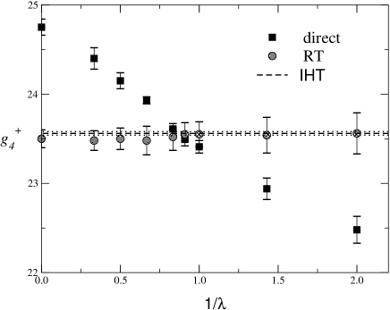
Figure 2: Estimates of $g_{4}^{+}$ obtained from an unbiased analysis (direct) of the HT series and from the analysis (RT) of the series obtained by means of the Roskies transform (2.2), for the $\phi^{4}$ lattice model. The dashed line marks the more precise estimate (with its error) derived from the analysis of an improved HT expansion in Ref. [243], $g_{4}^{+}=23.56(2)$.

In order to illustrate the role played by the nonanalytic corrections, we consider the zero-momentum four-point coupling $g_{4}$ defined in the high-temperature phase by

$$g_{4}\equiv-{3N\over N+2}{\chi_{4}\over\chi^{2}\xi^{d}},$$ (2.3)

which, in the critical limit, converges to the hyperuniversal constant $g_{4}^{+}$ defined in Table 2. In Fig. 2 we show some results concerning the three-dimensional Ising universality class. They were obtained in Ref. [240] from the analysis of the HT series of $g_{4}$ (using $\chi_{4}$ to 18th order) for the $\phi^{4}$ Hamiltonian (1.7) and several values of $\lambda$. We report an unbiased analysis (direct) and an analysis using the transformation (2.2) with $\Delta=1/2$ (RT). It is evident that the first type of analysis is unreliable, since one obtains an estimate of $g_{4}^{+}$ that is not independent of $\lambda$ within the quoted errors, which are obtained as usual from the spread of the approximants. For instance, the analysis of the series of the standard Ising model, corresponding to $\lambda=\infty$, gives results that differ by more than 5% from the estimate obtained from the second analysis, while the spread of the approximants is much smaller. The estimates obtained from the transformed series are independent of $\lambda$ within error bars, giving the estimate $g_{4}^{+}\approx 23.5$. Such independence clearly indicates that the transformation (2.2) is effectively able to take into account the nonanalytic behavior. Moreover, the result is in good agreement with the more precise estimate obtained using improved Hamiltonians, i.e. [243] $g_{4}^{+}=23.56(2)$ (see Sec. 3.3).

2.2 Monte Carlo methods

The Monte Carlo (MC) method is a powerful technique for the simulation of statistical systems. Its main advantage is its flexibility. Of course, results will be more or less precise depending on the efficiency of the algorithm. Systems with an $N$-vector order parameter and $O(N)$ symmetry are quite a special case, since there exists an efficient algorithm with practically no critical slowing down: the Wolff algorithm [1131], a generalization of the Swendsen-Wang algorithm [1045] for the Ising model (see Ref. [252] for a general discussion). The original algorithm was defined for the $N$-vector model, but it can be applied to general $O(N)$ models by simply adding a Metropolis test [193].

In this section we describe different methods for obtaining critical quantities from MC simulations. After discussing the standard infinite-volume methods, we present two successful techniques. One is based on real-space RG transformations, the second one makes use of the finite-size scaling (FSS) theory. Finally, we discuss nonequilibrium methods that represent a promising numerical technique for systems with slow relaxation.

2.2.1 Infinite-volume methods

Traditional MC simulations determine the critical behavior from infinite-volume data. In this case, the analysis of the MC data is done in two steps. In order to determine the critical behavior of a quantity $S$, one first computes ${S}(\beta,L)$ for fixed $\beta$ and several values of $L$ and determines

$${S}_{\infty}(\beta)=\lim_{L\to\infty}{S}(\beta,L),$$ (2.4)

by performing an extrapolation in $L$. For $L\to\infty$,

$${S}(\beta,L)\approx{S}_{\infty}(\beta)+aL^{p}\,e^{-L/\xi_{\rm gap}},$$ (2.5)

where $\xi_{\rm gap}$ is the exponential correlation length and $p$ an observable-dependent exponent. Such a rapid convergence usually makes the finite-size effects negligible compared to the statistical errors for moderately large values of $L/\xi_{\rm gap}$. In the HT phase a ratio $L/\xi_{\rm gap}\approx 5$-7 is usually sufficient, while in the LT phase larger values must be considered: for the three-dimensional Ising model, Ref. [272] used $L/\xi_{\rm gap}\approx 20$. Finite-size effects introduce a severe limitation on the values of $\xi_{\rm gap}$ that can be reached, since $L\lesssim 100$-200 in present-day three-dimensional MC simulations.

Once the infinite-volume quantities ${S}_{\infty}(\beta)$ are determined, exponents and amplitudes are obtained by fitting the numerical results to the corresponding expansion:

$${S}_{\infty}(\beta)=a|\beta_{c}-\beta|^{-\sigma}+b|\beta_{c}-\beta|^{-\sigma+\Delta}+\ldots$$ (2.6)

Of course, one cannot use too many unknown parameters in the fit and often only the leading term in Eq. (2.6) is kept. However, this is the origin of large systematic errors: It is essential to keep into account the leading nonanalytic correction with exponent $\Delta$.

Again, in order to show the importance of the nonanalytic scaling corrections, we present in Fig. 3 some numerical results [639, 85] for the four-point coupling $g_{4}$. A simple extrapolation of the MC data to a constant gives $g_{4}^{+}=24.5(2)$ [639] which is inconsistent with the result of Ref. [243], $g_{4}^{+}=23.56(2)$. On the other hand, a fit that takes into account the leading correction to scaling gives $g_{4}^{+}=23.7(2)$ [904], which is in agreement with the above-reported estimate.

Figure 3: MC results for the four-point coupling $g_{4}$ for the three-dimensional Ising model: (a) from Ref. [85]; (b) from Ref. [639]. For comparison we also report the extrapolation of the 18th-order HT series of Ref. [240] by means of a direct analysis ($\rm HT_{\rm direct}$) and of an analysis that uses the transformation (2.2) ($\rm HT_{RT}$). For each of these extrapolations we report two lines corresponding to the one-error-bar interval.

2.2.2 Monte-Carlo renormalization group

Here we briefly outline the real-space RG which has been much employed in numerical MC RG studies. This method has been amply reviewed in the literature, see, e.g., Refs. [1126, 1044].

The main idea of the RG approach is to reduce the number of degrees of freedom of the system by integrating out the short-range fluctuations. In the real-space RG this is performed by block-field transformations [599]. In a block-field transformation, a block with $l^{d}$ sites on the original lattice is mapped into a site of the blocked lattice. A block field $\phi_{B}$ is then constructed from the field $\phi$ of the original lattice, according to rules that should leave unchanged the critical modes, eliminating only the noncritical ones. The Hamiltonian ${\cal H}_{B}$ of the blocked system is defined as

$$\exp\left[-{\cal H}_{B}(\phi_{B})\right]=\int D\phi\,{\cal M}(\phi_{B},\phi)\exp\left[-{\cal H}(\phi)\right],$$ (2.7)

where ${\cal M}(\phi_{B},\phi)$ denotes the kernel of the block-field transformation. Then, the lattice spacing of the blocked lattice is rescaled to one.

RG transformations are defined in the infinite-dimensional space of all possible Hamiltonians. If ${\cal H}$ is written as

$${\cal H}(K_{1},K_{2},\ldots;O)=\sum_{a}K_{a}O_{a},$$ (2.8)

where $O_{a}$ are translation-invariant functions of the field $\phi$ and $K_{a}$ are the corresponding couplings, the RG transformation induces a mapping

$$K\rightarrow K^{\prime}=R(K).$$ (2.9)

The renormalized couplings $K^{\prime}$ are assumed to be analytic functions of the original ones.

The nonanalytic behavior at the critical point is obtained by iterating the RG transformation an infinite number of times. Continuous phase transitions are associated with the fixed points $K^{*}$ of the RG transformation. Critical exponents are determined by the RG flow in the neighborhood of the fixed point. If we define

$$T_{ab}=\left.\partial K^{\prime}_{a}\over\partial K_{b}\right|_{K=K^{*}},$$ (2.10)

the eigenvectors of $T$ give the linearized scaling fields. The corresponding eigenvalues can be written as $\lambda_{i}=l^{y_{i}}$, where $y_{i}$ are the RG dimensions of the scaling fields.

An exact RG transformation is defined in the space of Hamiltonians with an infinite number of couplings. However, in practice a numerical implementation of the method requires a truncation of the Hamiltonians considered. Therefore, any method that is based on real-space RG transformations chooses a specific basis, trying to keep those terms that are more important for the description of the critical modes. As a general rule, one keeps only terms with a small number of fields and that are localized (see, e.g., Ref. [157]). The precision of the method depends crucially on the choice for the truncated Hamiltonian and for the RG transformation.

In numerical MC studies, given a MC generated configuration $\{\phi\}$, one generates a series of blocked configurations $\{\phi^{(i)}\}$, with $i=0$ corresponding to the original configuration, by applying the block-field transformation. Correspondingly, one computes the operators $O^{(i)}\equiv O(\phi^{(i)})$. Then, one determines the matrices

$$\hskip-22.76228ptA_{ab}^{(i)}=\left\langle\left(O_{a}^{(i)}-\langle O_{a}^{(i)}\rangle\right)\left(O_{b}^{(i)}-\langle O_{b}^{(i)}\rangle\right)\right\rangle,$$

$$\hskip-22.76228ptB_{ab}^{(i)}=\left\langle\left(O_{a}^{(i)}-\langle O_{a}^{(i)}\rangle\right)\left(O_{b}^{(i-1)}-\langle O_{b}^{(i-1)}\rangle\right)\right\rangle$$ (2.11)

and the matrix $T^{(i)}$ [1043]

$$\sum_{b}A_{ab}^{(i)}T_{bc}^{(i)}=B_{ac}^{(i)}.$$ (2.12)

If all possible couplings were considered, the matrix $T^{(i)}$ would converge to $T$ defined in Eq. (2.10) for $i\to\infty$. In practice, only a finite number of couplings and a finite number of iterations is used. These approximations can be partially controlled by checking the convergence of the results with respect to the number of couplings and of RG iterations.

2.2.3 Finite-size scaling

Finite-size effects in critical phenomena have been the object of theoretical studies for a long time: see, e.g., Refs. [105, 930, 266, 265] for reviews. Only recently, due to the progress in the preparation of thin films, this issue has begun being investigated experimentally, see, e.g., Refs. [556, 690, 40, 41, 783, 92, 446, 366, 709, 644, 645]. FSS techniques are particularly important in numerical work. With respect to the infinite-volume methods, they do not need to satisfy the condition $\xi_{\rm gap}\ll L$. One can work with $\xi_{\rm gap}\sim L$ and thus is better able to probe the critical regime. FSS MC simulations are at present one of the most effective techniques for the determination of critical quantities. Here, we will briefly review the main ideas behind FSS and report several relations that have been used in numerical studies to determine the critical quantities.

The starting point of FSS is the generalization of Eq. (1.54) for the singular part of the Helmholtz free energy of a sample of linear size $L$ [416, 105, 931, 161]:

$${\cal F}_{\rm sing}(u_{t},u_{h},\{u_{i}\},L)=b^{-d}{\cal F}_{\rm sing}(b^{y_{t}}u_{t},b^{y_{h}}u_{h},\{b^{y_{i}}u_{i}\},L/b),$$ (2.13)

where $u_{t}\equiv u_{1}$, $u_{h}\equiv u_{2}$, $\{u_{i}\}$ with $i\geq 3$ are the scaling fields associated respectively with the reduced temperature, magnetic field, and the other irrelevant operators. Choosing $b=L$, we obtain

$${\cal F}_{\rm sing}(u_{t},u_{h},\{u_{i}\},L)=L^{-d}{\cal F}_{\rm sing}(L^{y_{t}}u_{t},L^{y_{h}}u_{h},\{L^{y_{i}}u_{i}\},1),$$ (2.14)

from which, by performing the appropriate derivatives with respect to $t$ and $H$, one finds the scaling behavior of the thermodynamically interesting quantities. We again assume that $u_{t}$ and $u_{h}$ are the only relevant scaling fields, and thus, neglecting correction of order $L^{y_{3}}=L^{-\omega}$, we can simply set $u_{i}=0$ in the previous equation. Using Eq. (2.14) one may obtain the FSS behavior of any thermodynamic quantity $S$. Considering $S(\beta,L)$ for $H=0$, if $S_{\infty}(\beta)\equiv S(\beta,\infty)$ behaves as $t^{-\sigma}$ for $t\rightarrow 0$, then we have

$$S(\beta,L)=L^{\sigma/\nu}\left[f_{S}\left(\xi_{\infty}/L\right)+O\left(L^{-\omega},\xi_{\infty}^{-\omega}\right)\right],$$ (2.15)

where $\xi_{\infty}(\beta)$ is the correlation length in the infinite-volume limit. We do not need to specify which definition we are using. For numerical studies, it is convenient to rewrite this relation in terms of a correlation length $\xi(\beta,L)$ defined in a finite lattice. Then, one may rewrite the above equation as

$$S(\beta,L)=L^{\sigma/\nu}\left[\bar{f}_{S}\left(\xi(\beta,L)/L\right)+O\left(L^{-\omega},\xi^{-\omega}\right)\right].$$ (2.16)

FSS methods can be used to determine $\beta_{c}$, critical exponents, and critical amplitudes. Below we will review a few of them (we assume everywhere $H=0$, but much can be generalized to $H\not=0$).

In order to determine $\beta_{c}$, a widely used method is the “crossing” method. Choose a thermodynamic quantity $S(\beta,L)$ for which $\sigma=0$ or $\sigma/\nu$ is known and define $R(\beta,L)\equiv S(\beta,L)L^{-\sigma/\nu}$. Then consider pairs $(L_{1},L_{2})$ and determine the solution $\beta_{\rm cross}$ of the equation [149]

$$R(\beta_{\rm cross},L_{1})=R(\beta_{\rm cross},L_{2}).$$ (2.17)

If $L_{1}$ and $L_{2}$ diverge, $\beta_{\rm cross}$ converges to $\beta_{c}$ with corrections of order $L_{1}^{-\omega-1/\nu}$, $L_{2}^{-\omega-1/\nu}$, and thus it provides an estimate of $\beta_{c}$. A widely used quantity is the Binder cumulant $Q$,

$$Q=\,{\langle M^{4}\rangle\over\langle M^{2}\rangle^{2}},$$ (2.18)

where $M$ is the magnetization. Other choices that have been considered are $\xi/L$, generalizations of the Binder cumulant using higher powers of the magnetization, and the ratio of the partition function with periodic and antiperiodic boundary conditions [520, 512, 233].

The determination of the critical exponents can be performed using several different methods. One of the oldest approaches is the phenomenological renormalization of Nightingale [853]. One fixes a temperature $\beta_{1}$ and two sizes $L_{1}$ and $L_{2}$ and then determines $\beta_{2}$ so that

$${\xi(\beta_{2},L_{2})\over\xi(\beta_{1},L_{1})}={L_{2}\over L_{1}}.$$ (2.19)

Neglecting scaling corrections, in the FSS regime $\beta_{1}$ and $\beta_{2}$ are related by

$$(\beta_{2}-\beta_{c})=\left({L_{1}\over L_{2}}\right)^{1/\nu}(\beta_{1}-\beta_{c}).$$ (2.20)

In Ref. [853] the method is implemented iteratively, using $L_{2}=L_{1}+1$. Starting from $\beta_{0}$, $L_{0}$, by using Eq. (2.20) one obtains a sequence of estimates $\beta_{i}$, $\nu_{i}$ that converge to $\beta_{c}$ and $\nu$ respectively. It is also possible to consider a magnetic field, obtaining in this case also the exponent $(\beta+\gamma)/\nu$.

Critical exponents can also be determined by studying thermodynamic quantities at the critical point. In this case,

$$S(\beta_{c},L)\sim L^{\sigma/\nu},$$ (2.21)

neglecting scaling corrections. Thus, one can determine $\sigma/\nu$ by simply studying the $L$-dependence. For example, $\gamma/\nu$ and $\beta/\nu$ can be determined from

$$\chi(\beta_{c},L)\sim L^{\gamma/\nu},\qquad|M|(\beta_{c},L)\sim L^{\beta/\nu}.$$ (2.22)

The exponent $\nu$ can be determined by studying the $L$-dependence of derivatives with respect to $\beta$. Indeed,

$$\left.{\partial S(\beta,L)\over\partial\beta}\right|_{\beta=\beta_{c}}\sim L^{(\sigma+1)/\nu},$$ (2.23)

which can be obtained from Eq. (2.15) using $\xi_{\infty}\sim|t|^{-\nu}$. This method has the drawback that an estimate of $\beta_{c}$ is needed. Moreover, since $\beta_{c}$ is usually determined only at the end of the runs, one must take into account the fact that the available numerical results correspond to $\beta\not=\beta_{c}$. There are then two possibilities: one may compute $S(\beta_{c},L)$ using the reweighting method [376, 395], or include correction terms proportional to $(\beta-\beta_{c})L^{1/\nu}$ in the fit Ansatz [161, 162]. In both cases, the method requires $(\beta-\beta_{c})L^{1/\nu}$ to be small. One may also consider $\beta_{c}$ as a free parameter and determine it by fitting $S(\beta,L)$ near the critical point [161, 162].

It is possible to avoid using $\beta_{c}$. In Refs. [93, 94, 95, 96, 98] one fixes $L_{1}$ and $L_{2}$ and then determines $\beta$, for instance by reweighting the data, so that

$${\xi(\beta,L_{1})\over\xi(\beta,L_{2})}={L_{1}\over L_{2}}.$$ (2.24)

Then, the exponent $\sigma$ is obtained from

$${S(\beta,L_{1})\over S(\beta,L_{2})}=\left({L_{1}\over L_{2}}\right)^{\sigma/\nu},$$ (2.25)

neglecting scaling corrections. When $L_{1}$ and $L_{2}$ go to infinity, this estimate converges towards the exact value. Due to the presence of cross-correlations, this method gives results that are more precise than those obtained by studying the theory at the critical point.

A somewhat different approach is proposed in Ref. [512]. One introduces an additional quantity $R(\beta,L)$ such that $R(\beta_{c},L)\to R^{*}$ for $L\to\infty$. Then, one fixes a value $\overline{R}$ —for practical purposes it is convenient to choose $\overline{R}\approx R^{*}$— and, for each $L$, determines $\beta_{f}(L)$ from

$$R(\beta_{f}(L),L)=\overline{R}.$$ (2.26)

Finally, one considers $S(\beta_{f}(L),L)$ which still behaves as $L^{\sigma/\nu}$ for large $L$. Due to the presence of cross-correlations, the error on $S$ at fixed $R$ turns out to be smaller than the error on $S$ at fixed $\beta$. With respect to the approach of Refs. [93, 94, 95, 96, 98], this method has the advantage of avoiding a tuning on two different lattices.

The FSS methods that we have described are effective in determining the critical exponents. However, they cannot be used to compute amplitude ratios or other infinite-volume quantities. For this purpose, however, one can still use FSS methods [743, 635, 250, 253, 785, 758, 114, 877, 390]. The idea consists in rewriting Eq. (2.16) as

$${S(\beta,sL)\over S(\beta,L)}=\hat{f}\left(\xi(\beta,L)/L\right)+O(L^{-\omega},\xi^{-\omega}),$$ (2.27)

where $s$ is an arbitrary (rational) number. In the absence of scaling corrections, one may proceed as follows. First, one performs several runs for fixed $L$, determining $S(\beta,sL)$, $S(\beta,L)$, $\xi(\beta,sL)$, and $\xi(\beta,L)$. By means of a suitable interpolation, this provides the function $\hat{f}(\xi(\beta,L)/L)$ for $S$ and $\xi$. Then, $S_{\infty}(\beta)$ and $\xi_{\infty}(\beta)$ are obtained from $S(\beta,L)$ and $\xi(\beta,L)$ by iterating Eq. (2.27) and the corresponding equation for $\xi(\beta,L)$. Of course, in practice one must be very careful about scaling corrections, increasing systematically $L$ till the results become independent of $L$ within error bars.

Finally, we note that scaling corrections represent the main source of error in all these methods. They should not be neglected in order to get reliable estimates of the critical exponents. The leading scaling correction, which is of order $O(L^{-\omega})$, is often important, and should be taken into account by performing fits with Ansatz

$$aL^{\sigma/\nu}+bL^{\sigma/\nu-\omega}.$$ (2.28)

As we have already stressed previously, these difficulties can be partially overcome if one uses an improved Hamiltonian. In this case the leading scaling corrections are absent and a naive fit to the leading behavior gives reliable results at the level of present-day statistical accuracy. However, in practice improved Hamiltonians are known only approximately, so that one may worry of the systematic error due to the residual correction terms. In Sec. 2.3.1 we will discuss how to keep this systematic error into account.

2.2.4 Dynamic methods

Nonequilibrium dynamic methods are numerical techniques that compute static and dynamic critical exponents by studying the relaxation process towards equilibrium. They are especially convenient in systems with slow dynamics, since they allow the determination of the critical exponents without ever reaching thermal equilibrium. Two slighly different techniques have been developed: the nonequilibrium-relaxation (NER) method, see Refs. [565, 567, 859, 566, 873] and references therein, and the short-time critical dynamics (STCD) method, see Refs. [700, 701, 738, 991] and references therein.

In the NER method one studies the long-time relaxation towards equilibrium. In this limit, the nonequilibrium free energy scales as [1036]

$${\cal F}(t,H,L,\tau)=L^{-d}\widehat{F}(tL^{y_{t}},HL^{y_{h}},\tau L^{z}),$$ (2.29)

where $\tau$ is the dynamics time, $z$ is a new critical exponent, and subleading corrections have been omitted. The method bears some similarities with the FSS methods described before. One first determines the critical point, and then studies the dynamics at criticality determining the exponents from the large-time (instead of large-$L$) behavior of correlation functions. Since one does not need to reach equilibrium, large volumes can be considered. Moreover, since correlations increase with increasing $\tau$, one can avoid finite-size effects by stopping the dynamics when the correlation length is some fraction of the size. In order to determine the critical point, one may monitor the behavior of the time-dependent magnetization $m(t,\tau)$. For $t\not=0$, $m(t,\tau)$ converges to its asymptotic value exponentially, while at the critical point $m(0,\tau)\sim\tau^{-\beta/(z\nu)}$. It suffices to consider

$$f(t,\tau)={d\ln m(t,\tau)\over d\ln\tau}$$ (2.30)

that diverges for $t>0$, goes to zero for $t<0$, and converges to a constant for $t=0$. Once $T_{c}$ is determined, the critical exponents can be obtained from the behavior of powers of $m(t,\tau)$ and of their derivatives with respect to $t$ at the critical point.

The STDC method is similar and uses again dynamic scaling. Here, one assumes that, besides the universal behavior in the long-time regime, there exists another universal stage of the relaxation at early (macroscopic) times. The scaling behavior of this regime has been shown for the dynamics of model A in Ref. [585], but it is believed to be a general characteristic of dynamic critical phenomena.

2.3 Improved Hamiltonians

As we already stressed, one of the main sources of systematic errors is the presence of nonanalytic corrections controlled by the RG eigenvalue $y_{3}=-\omega$. A way out exploits improved models, i.e. models for which there are no corrections with exponent $\omega$: No terms of order $|t|^{\omega\nu}=|t|^{\Delta}$ appear in infinite-volume quantities and no terms of order $L^{-\omega}$ in FSS variables. Such Hamiltonians cannot be determined analytically and one must use numerical methods. Some of them will be presented below.

2.3.1 Determinations of the improved Hamiltonians

In order to determine an improved Hamiltonian, one may consider a one-parameter family of models, parametrized, say, by $\lambda$, that belong to the given universality class. Then, one may consider a specific quantity and find numerically a value $\lambda^{*}$ for which the leading correction to scaling is absent. According to RG theory, at $\lambda^{*}$ the leading scaling correction gets suppressed in any quantity. Note that, within a given one-parameter family of models, nothing guarantees that such a value of $\lambda$ can be found. For instance, in the large-$N$ limit of the lattice $\phi^{4}$ theory (1.7) no positive value of $\lambda$ exists that achieves the suppression of the leading scaling corrections [240]. For a discussion in the continuum, see, e.g., Refs. [73, 1152].

The first attempt to exploit improved Hamiltonians is due to Chen, Fisher, and Nickel [288]. They studied two classes of two-parameter models, the bcc scalar double-Gaussian and Klauder models, that are expected to belong to the Ising universality class and that interpolate between the spin-$1/2$ Ising model and the Gaussian model. They showed that improved models with suppressed leading corrections to scaling can be obtained by tuning the parameters (see also Refs. [419, 844]). The main difficulty of the method is the precise determination of $\lambda^{*}$. In Refs. [288, 457] the partial differential approximant technique was used; however, the error on $\lambda^{*}$ was relatively large, and the final results represented only a modest improvement with respect to standard (and much simpler) analyses using biased approximants.

One may determine the improved Hamiltonian by comparing the results of a “good” and of a “bad” analysis of the HT series [419, 240]. Considering again the zero-momentum four-point coupling $g_{4}$, we can for instance determine $\lambda^{*}$ from the results of the analyses presented in Sec. 2.1. The improved model corresponds to the value of $\lambda$ for which the unbiased analysis gives results that are consistent with the analysis that takes into account the subleading correction. From Fig. 2, we see that in the interval $1.0<\lambda<1.2$ the two analyses coincide and thus, we can estimate $\lambda^{*}=1.1(1)$. This estimate is consistent with the result of Ref. [512], i.e. $\lambda^{*}=1.10(2)$ obtained using the MC method based on FSS, but is much less precise.

In the last few years many numerical studies [161, 520, 96, 98, 512, 513, 515, 233, 234] have shown that improved Hamiltonians can be accurately determined by means of MC simulations, using FSS methods.

There are several methods that can be used. A first class of methods is very similar in spirit to the crossing technique employed for the determination of $\beta_{c}$. In its simplest implementation [240] one considers a quantity $R(\beta,\lambda,L)$ such that, for $L\to\infty$, $R(\beta_{c}(\lambda),\lambda,L)$ converges to a universal constant $R^{*}$, which is supposed to be known. Standard scaling arguments predict for $L\to\infty$

$$R(\beta_{c}(\lambda),\lambda,L)\approx R^{*}+a_{1}(\lambda)L^{-\omega}+a_{2}(\lambda)L^{-2\omega}+\ldots+b_{1}(\lambda)L^{-\omega_{2}}\ldots$$ (2.31)

where $\omega_{2}\equiv-y_{4}$ is the next-to-leading correction-to-scaling exponent. In order to evaluate $\lambda^{*}$, which is the value for which $a_{1}(\lambda)=0$, one can determine $\lambda^{\rm eff}(L)$ from the equation

$${R}(\beta_{c}(\lambda^{\rm eff}(L)),\lambda^{\rm eff}(L),L)={R}^{*},$$ (2.32)

where we assume $R^{*}$ and $\beta_{c}(\lambda)$ to be known. For $L\to\infty$, $\lambda^{\rm eff}(L)$ converges to $\lambda^{*}$ with corrections of order $L^{\omega-\omega_{2}}$. In practice, neither $R^{*}$ nor $\beta_{c}(\lambda)$ are known exactly. It is possible to avoid these problems by considering two different quantities $R_{1}$ and $R_{2}$ that have a universal limit for $L\to\infty$ [512, 233]. First, we define $\beta_{f}(\lambda,L)$ by

$$R_{1}(\beta_{f},\lambda,L)=\bar{R}_{1},$$ (2.33)

where $\bar{R}_{1}$ is a fixed value taken from the range of $R_{1}$. Approximate estimates of $\lambda^{*}$ are then obtained by solving the equation

$${R}_{2}(\beta_{f}(\lambda,L),\lambda,L)={R}_{2}(\beta_{f}(\lambda,bL),\lambda,bL).$$ (2.34)

for some value of $b$.

Alternatively [96, 98, 512, 521, 233], one may determine the size of the corrections to scaling for two values of $\lambda$ which are near to $\lambda^{*}$, but not too near in order to have a good signal, and perform a linear interpolation. In the implementation of Refs. [96, 98] one considers the corrections to Eq. (2.25), while Refs. [512, 521, 233] consider the corrections to a RG-invariant quantity at fixed $\beta_{f}$, see Eq. (2.33).

We should note that all these numerical methods provide only approximately improved Hamiltonians. Therefore, leading corrections with exponent $\omega$ are small but not completely absent. However, it is possible to evaluate the residual systematic error due to these terms. The idea is the following [512]. First, one considers a specific quantity that behaves as

$$S(L)=aL^{\sigma/\nu}(1+b(\lambda)L^{-\omega}+\ldots).$$ (2.35)

Then, one studies numerically $S(L)$ in the approximately improved model, i.e. for $\lambda=\lambda^{*}_{\rm est}$ ($\lambda^{*}_{\rm est}$ is the estimated value of $\lambda^{*}$), and in a model in which the corrections to scaling are large: for instance in the $N$-vector model corresponding to $\lambda=\infty$. Finally, one determines numerically an upper bound on $b(\lambda^{*}_{\rm est})/b(\infty)$. RG theory guarantees that this ratio is identical for any quantity. Therefore, one can obtain an upper bound on the residual irrelevant corrections, by computing the correction term in the $N$-vector model—this is easy since corrections are large—and multiplying the result by the factor determined above.

2.3.2 List of improved Hamiltonians

We list here the improved models that have been determined so far. We write the partition function in the form

$$Z=\int\prod_{i}\,d\mu(\phi_{i})\exp\left[\beta\sum_{<ij>}\phi_{i}\cdot\phi_{j}\right],$$ (2.36)

where $\phi_{i}$ is an $N$-dimensional vector and the sum is extended over all nearest-neighbor pairs $<ij>$. For $N=1$ the following improved models have been determined:

1. Double-Gaussian model:

   $$d\mu(\phi)=d\phi\,\left\{\exp\left[-{(\phi+\sqrt{y})^{2}\over 2(1-y)}\right]+\exp\left[-{(\phi-\sqrt{y})^{2}\over 2(1-y)}\right]\right\},$$ (2.37)

   with $0<y<1$. The improved model has been determined on the bcc lattice from the study of HT series. The improved model corresponds to $y^{*}=0.87(4)$ [288], $y^{*}=0.87(1)$ [457], $y^{*}=0.90(3)$ [419], $y^{*}\approx 0.85$ [844].

2. Klauder model:

   $$d\mu(\phi)=\,d\phi\,|\phi|^{y/(1-y)}\exp\left(-{\phi^{2}\over 2(1-y)}\right),$$ (2.38)

   with $0<y<1$. The improved model has been determined on the bcc lattice from the study of HT series. The improved model corresponds to $y^{*}=0.81(6)$ [288], $y^{*}=0.815(35)$ [419].

3. $\phi^{4}$-$\phi^{6}$ model:

   $$d\mu(\phi)=\,d\phi\,\exp\left[-\phi^{2}-\lambda(\phi^{2}-1)^{2}-\lambda_{6}(\phi^{2}-1)^{3}\right].$$ (2.39)

   The couplings corresponding to improved models have been determined by means of MC simulations. On the sc lattice, the Hamiltonian is improved for these values of the couplings: (a) $\lambda^{*}=1.10(2)$, $\lambda_{6}^{*}=0$ [512]; (b) $\lambda^{*}=1.90(4)$, $\lambda_{6}^{*}=1$ [240].

4. Blume-Capel model:

   $$d\mu(\phi)=\,d\phi\,\left[\delta(\phi-1)+\delta(\phi+1)+e^{D}\delta(\phi)\right].$$ (2.40)

   On the sc lattice the Hamiltonian is improved for $D^{*}\approx 0.7$ [161], $D^{*}=0.641(8)$ [513].

For $N=2,3,4$ and for the $\phi^{4}$ theory (1.7) on a simple cubic lattice, $\lambda^{*}$ has been determined by means of FSS MC simulations [521, 233, 234, 515]. The estimates of $\lambda^{*}$ are the following [233, 234, 515]:

$$\hskip-28.45274pt\lambda^{*} = 2.07(5)\hphantom{2.}\qquad\qquad\hbox{\rm for $N=2$},$$ (2.41)

$$\hskip-28.45274pt\lambda^{*} = 4.6(4)\hphantom{22.}\qquad\qquad\hbox{\rm for $N=3$},$$ (2.42)

$$\hskip-28.45274pt\lambda^{*} = 12.5(4.0)\qquad\qquad\hbox{\rm for $N=4$}.$$ (2.43)

For $N=2$ the dynamically dilute XY model has also been considered:

$$d\mu(\phi)=\,d^{2}\phi\,\left[\delta(\phi_{1})\delta(\phi_{2})+{e^{D}\over 2\pi}\delta(1-|\phi|)\right],$$ (2.44)

where $\phi=(\phi_{1},\phi_{2})$. The Hamiltonian is improved for $D^{*}=1.02(3)$ [233]. Again, the improved theory has been determined by means of MC simulations.

Also models with extended interactions have been considered, such as [161, 520]

$${\cal H}=\beta\Bigl{[}\sum_{<ij>}\sigma_{i}\sigma_{j}+y\sum_{[ij]}\sigma_{i}\sigma_{j}\Bigr{]},$$ (2.45)

where $\sigma_{i}=\pm 1$, the first sum is extended over all nearest-neighbor pairs $<ij>$, and the second one over all third nearest-neighbor pairs $[ij]$. In Ref. [161] a significant reduction of the subleading corrections was observed for $y\approx 0.4$. However, the subsequent analysis of Ref. [520] found $y^{*}\mathrel{\hbox to0.0pt{\lower 3.0pt\hbox{$\mathchar 536\relax$}\hss}\raise 2.0pt\hbox{$\mathchar 316\relax$}}0.25$.

2.4 Field-theoretical methods

Field-theoretical methods can be divided into two classes: (a) perturbative approaches based on the $\phi^{4}$ continuum Hamiltonian

$${\cal H}=\int d^{d}x\left[{1\over 2}\partial_{\mu}\phi(x)\partial_{\mu}\phi(x)+{r\over 2}\phi(x)^{2}+{u\over 4!}\phi(x)^{4}\right];$$ (2.46)

(b) nonpertubative approaches based on approximate solutions of Wilson’s RG equations.

The oldest perturbative method is the $\epsilon$ expansion in which the expansion parameter is $\epsilon=4-d$ [1125]. Subsequently, Parisi [880] pointed out the possibility of using pertubation theory directly at the physical dimensions $d=3$ and $d=2$. In the original works [87, 880] the theory was renormalized at zero momentum. Later, a four-dimensional minimal subtraction scheme without $\epsilon$ expansion was also proposed [342, 984, 985]. With a slight abuse of language, we will call the first “traditional” method as the fixed-dimension expansion approach, although also in the second case the dimension is fixed. The second approach will be named the minimal subtraction scheme without $\epsilon$ expansion.

The nonperturbative approach has a very long history [1106, 1126, 465, 835, 836] and it has been the subject of extensive work even recently, see, e.g., Refs. [803, 134, 77] and references therein. A brief discussion will be presented here. We only mention that for $O(N)$ vector models the estimates of the critical parameters are less precise than those obtained in studies using perturbative approaches.

2.4.1 The fixed-dimension expansion

In the fixed-dimension expansion one works directly in $d=3$ or $d=2$. In this case the theory is super-renormalizable since the number of primitively divergent diagrams is finite. One may regularize the corresponding integrals by keeping $d$ arbitrary and performing an expansion in $\epsilon=3-d$ or $\epsilon=2-d$. Poles in $\epsilon$ appear in divergent diagrams. Such divergences are related to the necessity of performing an infinite renormalization of the parameter $r$ appearing in the bare Hamiltonian, see, e.g., the discussion in Ref. [71]. This problem can be avoided by replacing $r$ with the mass $m$ defined by

$$m^{-2}=\,{1\over\Gamma^{(2)}(0)}\,\left.{\partial\Gamma^{(2)}(p^{2})\over\partial p^{2}}\right|_{p^{2}=0},$$ (2.47)

where the function $\Gamma^{(2)}(p^{2})$ is related to the one-particle irreducible two-point function by

$$\Gamma^{(2)}_{ab}(p)=\delta_{ab}\Gamma^{(2)}(p^{2}).$$ (2.48)

Perturbation theory in terms of $m$ and $u$ is finite. The critical limit is obtained for $m\to 0$. To handle it, one considers appropriate RG functions. Specifically, one defines the zero-momentum four-point coupling $g$ and the field-renormalization constant $Z_{\phi}$ by

$$\Gamma^{(2)}_{ab}(p)=\delta_{ab}Z_{\phi}^{-1}\left[m^{2}+p^{2}+O(p^{4})\right],$$ (2.49)

$$\Gamma^{(4)}_{abcd}(0)=Z_{\phi}^{-2}m^{4-d}{g\over 3}\left(\delta_{ab}\delta_{cd}+\delta_{ac}\delta_{bd}+\delta_{ad}\delta_{bc}\right),$$ (2.50)

where $\Gamma^{(n)}_{a_{1},\ldots,a_{n}}$ are one-particle irreducible correlation functions. Then, one defines a coupling-renormalization constant $Z_{u}$ and a mass-renormalization constant $Z_{t}$ by

$$u=m^{4-d}gZ_{u}Z_{\phi}^{-2},\qquad\Gamma^{(1,2)}_{ab}(0)=\,\delta_{ab}Z_{t}^{-1},$$ (2.51)

where $\Gamma^{(1,2)}_{ab}(p)$ is the one-particle irreducible two-point function with an insertion of ${1\over 2}\phi^{2}$. The renormalization constants are determined as perturbative expansions in powers of $g$. The fixed point of the model is determined by the nontrivial zero $g^{*}$ of the $\beta$-function

$$\beta(g)=m\left.{\partial g\over\partial m}\right|_{u}=(d-4)g\left[1+g{d\over dg}\log(Z_{u}Z_{\phi}^{-2})\right]^{-1}.$$ (2.52)

Note that the fixed-point value $g^{*}$ coincides with the critical value $g_{4}^{+}$ of $g_{4}$, cf. Eq. (2.3). Then, one defines

$$\hskip-28.45274pt\eta_{\phi}(g) = \left.{\partial\ln Z_{\phi}\over\partial\ln m}\right|_{u}=\beta(g){\partial\ln Z_{\phi}\over\partial g},$$ (2.53)

$$\hskip-28.45274pt\eta_{t}(g) = \left.{\partial\ln Z_{t}\over\partial\ln m}\right|_{u}=\beta(g){\partial\ln Z_{t}\over\partial g}.$$ (2.54)

Finally, the critical exponents are given by

$$\eta = \eta_{\phi}(g^{*}),$$ (2.55)

$$\nu = \left[2-\eta_{\phi}(g^{*})+\eta_{t}(g^{*})\right]^{-1},$$ (2.56)

$$\omega = \beta^{\prime}(g^{*}),$$ (2.57)

where $\omega$ is the exponent associated with the leading irrelevant operator. All other exponents can be obtained using the scaling and hyperscaling relations.

Since this method is based on zero-momentum renormalization conditions, it is not well suited for the study of vector models in the LT phase. In this case, the minimal-subtraction scheme without $\epsilon$ expansion can be used. Since it is strictly related to the $\epsilon$ expansion, it will be presented in the next section.

The longest available series for the critical exponents can be found in Refs. [87, 821, 56] for $d=3$ and in Ref. [870] for $d=2$. More precisely, in three dimensions the critical exponents and the $\beta$-function are known to six loops for generic values of $N$ [56]. For $N=0,1,2,3$ seven-loop series for $\eta_{\phi}$ and $\eta_{t}$ were computed in Ref. [821]. They are reported in the Appendix of Ref. [481]. In two dimensions, five-loop series are available for all values of $N$ [870]. Perturbative expansions of some universal amplitude ratios involving HT quantities and of the $2n$-point renormalized coupling constants $g_{2n}^{+}$ can be found in Refs. [71] and [1022] respectively. For the scalar theory an extension of the method [79] allowed to obtain the free energy below the critical temperature and therefore all universal amplitude ratios defined from zero-momentum quantities. For the study of the LT phase of the Ising model, a slightly different approach was developed in Refs. [819, 484], which also allowed the computation of ratios involving the correlation length.

2.4.2 The $\epsilon$ expansion

The $\epsilon$ expansion [1125] is based on the observation that, for $d=4$, the theory is essentially Gaussian. One considers the standard perturbative expansion, and then transforms it into an expansion in powers of $\epsilon\equiv 4-d$. In practice, the method works as in the fixed-dimension expansion. One first determines the expansion of the renormalization constants $Z_{u}$, $Z_{\phi}$, and $Z_{t}$ in powers of the coupling $g$. Initially, they were obtained by requiring the normalization conditions (2.49), (2.50), and (2.51). However, in this framework it is simpler to use the minimal-subtraction scheme [1053]. Once the renormalization constants are determined, one computes the RG functions $\beta(g)$, $\eta_{\phi}(g)$, and $\eta_{t}(g)$ as in Sec. 2.4.1. The fixed-point value $g^{*}$ is obtained by solving the equation $\beta(g^{*})=0$ perturbatively in $\epsilon$. Once the expansion of $g^{*}$ is available, one obtains the expansion of the exponents, by expressing $\eta_{\phi}(g^{*})$ and $\eta_{t}(g^{*})$ in powers of $\epsilon$. Notice that, in the minimal-subtraction scheme, $g$ is not related to $g_{4}$.

In this scheme, five-loop series for the exponents were computed in Refs. [294, 657]. The equation of state and several amplitude ratios were determined in Refs. [182, 1096, 847, 137, 907].

The minimal-subtraction scheme without $\epsilon$ expansion [342, 984, 985] is strictly related. The functions $\beta(g)$, $\eta_{\phi}(g)$, and $\eta_{t}(g)$ are the minimal-subtraction functions. However, here $\epsilon$ is no longer considered as a small quantity but it is set to its physical value, i.e. in three dimensions one simply sets $\epsilon=1$. Then, the procedure is identical to that presented for the fixed-dimension expansion. A nontrivial zero $g^{*}$ of the $\beta$-function is determined and the exponent series are computed for this value of $g^{*}$. The method is well suited for the study of universal LT properties of vector systems, and indeed, perturbative series for several amplitude ratios have been computed [208, 686, 1032, 1033].

2.4.3 Resummation of the perturbative series

FT perturbative expansions are divergent. Thus, in order to obtain accurate results, an appropriate resummation is required. This can be done by exploiting their Borel summability, that has been proved for the fixed-dimension expansion of the $O(N)$ $\phi^{4}$ theory in $d<4$ [360, 752, 381, 751] and has been conjectured for the $\epsilon$ expansion. If we consider a quantity $S(g)$ that has a perturbative expansion

$$S(g)\approx\sum s_{k}g^{k},$$ (2.58)

the large-order behavior of the coefficients is given by

$$s_{k}\sim k!\,(-a)^{k}\,k^{b}\,\left[1+O(k^{-1})\right],$$ (2.59)

with $a>0$. Here, the perturbative coupling is the renormalized coupling constant of the fixed-dimension expansion, but the same discussion applies to the $\epsilon$ expansion, replacing $g$ by $\epsilon$. Note that the value of the constant $a$ is independent of the particular quantity considered, unlike the constant $b$. The constants $a$ and $b$ can be determined by means of a steepest-descent calculation in which the relevant saddle point is a finite-energy solution (instanton) of the classical field equations with negative coupling [710, 180], see also Refs. [1152, 883].

In order to resum the perturbative series, we introduce the Borel-Leroy transform $B(t)$ of $S(g)$,

$$S(g)=\int_{0}^{\infty}t^{c}e^{-t}B(t),$$ (2.60)

where $c$ is an arbitrary number. Its series expansion is given by

$$B_{\rm exp}(t)=\sum_{k}{s_{k}\over\Gamma(k+c+1)}t^{k}.$$ (2.61)

The constant $a$ that characterizes the large-order behavior of the original series is related to the singularity $t_{s}$ of the Borel transform $B(t)$ that is nearest to the origin: $t_{s}=-1/a$. The series $B_{\rm exp}(t)$ is convergent in the disk $|t|<|t_{s}|=1/a$ of the complex plane, and also on the boundary if $c>b$. In this domain, one can compute $B(t)$ using $B_{\rm exp}(t)$. However, in order to compute the integral (2.60), one needs $B(t)$ for all positive values of $t$. It is thus necessary to perform an analytic continuation of $B_{\rm exp}(t)$.

The analytic continuation may be achieved using [87] Padé approximants to the series (2.61). A more refined procedure exploits the knowledge of the large-order behavior of the expansion, and in particular of the constant $a$. One performs an Euler transformation [693]

$$y(t)={\sqrt{1+at}-1\over\sqrt{1+at}+1},$$ (2.62)

that allows to rewrite $B(t)$ in the form

$$B(t)=\sum_{k}f_{k}\,[y(t)]^{k}.$$ (2.63)

If all the singularities belong to the real interval $[-\infty,-t_{c}]$, the expansion (2.63) converges everywhere in the complex $t$-plane except on the negative axis for $t<-t_{c}$. After these transformations, one obtains a new expansion for the function $S(g)$:

$$S(g)\approx\int^{\infty}_{0}dt\,e^{-t}t^{c}\,\sum_{k}f_{k}\,[y(tg)]^{k}.$$ (2.64)

This sequence of operations has transformed the original divergent series into an integral of a convergent one, which can then be studied numerically. Notice that the convergence of the integral (2.64), that is controlled by the analytic properties of $S(g)$, is not guaranteed. For instance, if $S(g)$ has a cut for $g\geq g^{*}$—we will show below that this occurs in the fixed-dimension expansion—then the integral does not converge for $g>g^{*}$.

We mention that one may also use Eq. (2.63) when $a$ is not known, considering $a$ as a free parameter that can be optimized in the resummation procedure [810].

A different resummation method is used by Kleinert [653, 654, 587]. Instead of using the perturbative series in terms of the renormalized coupling constant $g$, he considers the expansion in terms of the bare coupling $u$. Since perturbative series in three dimensions are expressed in terms of $\overline{u}=u/m$, the critical results are obtained by evaluating the perturbative expressions in the limit $\overline{u}\to\infty$. Similar extrapolations are used in the context of polymers, i.e. in the $\phi^{4}$ theory in the limit $N\to 0$; see, e.g., Ref. [332]. Of course, the extrapolation is here a tricky point. Refs. [653, 654] use a variational method. Essentially, one introduces a new parameter such that the exact expressions are independent of it. In the truncated series the new parameter is a nontrivial variable that is fixed by requiring the results to be stationary with respect to its variation. The variational method transforms an initially divergent series in a convergent sequence of approximations.

The convergence of all the resummation methods depends on the analytic behavior at $g=g^{*}$. In particular, the convergence may be rather slow if the resummed function is nonanalytic at $g^{*}$.

Singularities—predicted long ago in Refs. [880, 838, 839]—appear in the fixed-dimension expansion renormalized at zero momentum. To understand the problem, following Nickel [838], let us consider the zero-momentum four-point coupling $g_{4}$—as we already remarked, it coincides with the perturbative coupling $g$ defined in Eq. (2.50)—as a function of the reduced temperature $t$. For $t\to 0$ we can write down an expansion of the form

$$g_{4}=g^{+}_{4}\,\Bigl{[} \hskip-14.22636pt1+a_{1}t+a_{2}t^{2}+\ldots+b_{1}t^{\Delta}+b_{2}t^{2\Delta}+\ldots$$ (2.65)

$$\hskip-14.22636pt+c_{1}t^{\Delta+1}+\ldots+d_{1}t^{\Delta_{2}}+\ldots+e_{1}t^{\gamma}+\ldots\Bigr{]}\;,$$

where $\Delta$, $\Delta_{2}$, $\ldots$ are subleading exponents. The correction proportional to $t^{\gamma}$ is due to the presence of an analytic background in the free energy.

Starting from Eq. (2.65), one may easily compute the $\beta$-function. Since the mass gap $m$ scales analogously, one obtains the following expansion:

$$\beta(g_{4})\equiv m{\partial g_{4}\over\partial m}= \hskip-14.22636pt\alpha_{1}\Delta g+\alpha_{2}(\Delta g)^{2}+\ldots+\beta_{1}(\Delta g)^{1\over\Delta}+\beta_{2}(\Delta g)^{2\over\Delta}+\ldots$$ (2.66)

$$\hskip-14.22636pt+\gamma_{1}(\Delta g)^{1+{1\over\Delta}}+\ldots+\delta_{1}(\Delta g)^{\Delta_{2}\over\Delta}+\ldots+\zeta_{1}(\Delta g)^{\gamma\over\Delta}+\ldots,$$

where $\Delta g=g^{+}_{4}-g_{4}$. Eq. (2.66) clearly shows the presence of several nonanalytic terms with exponents depending on $1/\Delta$, $\Delta_{i}/\Delta$, and $\gamma/\Delta$.

As pointed out by Sokal [1020, 698] (see also Ref. [76] for a discussion in Wilson’s RG setting), the nonanalyticity of the RG functions can also be understood within Wilson’s RG approach. We repeat his argument here. Consider the Gaussian fixed point which, for $3\leq d<4$, has a two-dimensional unstable manifold ${\cal M}_{u}$: The two unstable directions correspond to the interactions $\phi^{2}$ and $\phi^{4}$. The continuum field theories are in a one-to-one correspondence with Hamiltonians on ${\cal M}_{u}$. Thus, the FT RG is nothing but Wilson’s RG restricted to ${\cal M}_{u}$. The point is that there is no reason why it should approach the fixed point along a direction orthogonal to all other subleading irrelevant operators. Barring miracles, the approach should have nonzero components along any of the irrelevant directions. But, if this happens, nonanalytic terms are present in any RG function.

This issue has been investigated in the framework of the $1/N$ expansion [904], computing the asymptotic behavior of $\beta(g)$ for $g\to g^{*}$ to next-to-leading order in $1/N$ and for $2<d<4$. The result shows that nonanalytic terms are present consistently with Eq. (2.66). Indeed, corrections of order $(\Delta g)^{1+1/\Delta}$ and/or $(\Delta g)^{\Delta_{2}/\Delta}$ appear. No term proportional to $(\Delta g)^{1/\Delta}$ is found, which implies $a_{1}=0$ in Eq. (2.65). In Ref. [223] the computation is extended to two dimensions, finding again nonanalytic terms.

These singularities may cause a slow convergence in the resummations of the perturbative series. In Refs. [223, 280] some simple test functions were considered and it was shown that large discrepancies should be expected if the first nonanalytic exponent is small. For instance, if a function $f(g)$ behaves as the $\beta$ function, i.e.

$$f(g)\approx a(g-g_{0})+b(g-g_{0})^{1+p}$$ (2.67)

for $g\to g_{0}$, a relatively precise estimate of $a$ is obtained if $p\mathrel{\hbox to0.0pt{\lower 3.0pt\hbox{$\mathchar 536\relax$}\hss}\raise 2.0pt\hbox{$\mathchar 318\relax$}}1$, while for small values of $p$ the estimate is largely incorrect and, even worse, the errors, which are obtained as usual by stability criteria, are far too small. It is important to note that these discrepancies are not related to the fact that the series are divergent. They would be present even if the perturbative expansions were convergent.

Of course, the interesting question is whether these nonanalyticities are relevant in the $\phi^{4}$ perturbative series. In three dimensions and for $N=0,1,2,3$, $\Delta\approx 0.5$ and $\Delta_{2}/\Delta$ is approximately 2 [465, 836]. Thus, the leading nonanalytic term has exponent $\Delta_{2}/\Delta$ and is rather close to an analytic one. Therefore, we expect small effects in three dimensions, and indeed the FT results are in substantial agreement with the estimates obtained in MC and HT studies. The situation worsens in the two-dimensional case. In the Ising model Ref. [223] predicted a nonanalytic term $(\Delta g)^{8/7}$, while for $N\geq 3$ logarithmic corrections, such as $(\Delta g)/\log\,\Delta g$, are predicted on general grounds and found explicitly in a large-$N$ calculation [223]. Since the first nonanalytic term has a small exponent, large deviations are expected [223]. Indeed, two-dimensional estimates differ significantly from the theoretically expected results [693, 870].

On the other hand, for the $\epsilon$ expansion it has been argued that no nonanalyticities are present in universal quantities. This has also been argued for the fixed-dimension expansion in the minimal subtraction scheme [981, 74], but it is difficult to verify in the absence of a nonperturbative definition of the scheme.

Finally, we mention that it is possible to improve the $\epsilon$-expansion results for a quantity $R$ if its value is known for some values of the dimensions. The method was originally proposed in Refs. [695, 331, 334] where exact values in two or one dimension were used in the analysis of the $\epsilon$ expansion. The method of Ref. [695] works as follows. One considers a quantity $R$ such that for $\epsilon=\epsilon_{1}$ the exact value $R_{\rm ex}(\epsilon_{1})$ is known. Then, one defines

$$\overline{R}(\epsilon)=\left[{R(\epsilon)-R_{\rm ex}(\epsilon_{1})\over(\epsilon-\epsilon_{1})}\right],$$ (2.68)

and a new quantity

$$R_{\rm imp}(\epsilon)=R_{\rm ex}(\epsilon_{1})+(\epsilon-\epsilon_{1})\overline{R}(\epsilon).$$ (2.69)

New estimates of $R$ at $\epsilon=1$ can then be obtained by resumming the $\epsilon$ expansion of $\overline{R}(\epsilon)$ and then computing $R_{\rm imp}(1)$. The idea behind this method is very simple. If, for instance, the value of $R$ for $\epsilon=2$ is known, one uses as zeroth-order approximation at $\epsilon=1$ the value of the linear interpolation between $\epsilon=0$ and $\epsilon=2$ and then uses the series in $\epsilon$ to compute the deviations. If the interpolation is a good approximation, one should find that the series that gives the deviations has smaller coefficients than the original one. Consequently, also the errors in the resummation are reduced.

In Ref. [904] this strategy was generalized to the case in which one knows the exact value of $R$ for more than one value of $\epsilon$. If exact values $R_{\rm ex}(\epsilon_{1})$, $\ldots$, $R_{\rm ex}(\epsilon_{k})$ are known for a set of dimensions $\epsilon_{1}$, $\ldots$, $\epsilon_{k}$, $k\geq 2$, then one defines

$$Q(\epsilon)=\sum_{i=1}^{k}\left[{R_{\rm ex}(\epsilon_{i})\over(\epsilon-\epsilon_{i})}\prod_{j=1,j\not=i}^{k}(\epsilon_{i}-\epsilon_{j})^{-1}\right],$$ (2.70)

and

$$\overline{R}(\epsilon)={R(\epsilon)\over\prod_{i=1}^{k}(\epsilon-\epsilon_{i})}-Q(\epsilon),$$ (2.71)

and finally

$$R_{\rm imp}(\epsilon)=\left[Q(\epsilon)+\overline{R}(\epsilon)\right]\prod_{i=1}^{k}(\epsilon-\epsilon_{i}).$$ (2.72)

One can easily verify that the expression

$$\left[Q(\epsilon)+\overline{R}(0)\right]\prod_{i=1}^{k}(\epsilon-\epsilon_{i})$$ (2.73)

represents the $k$th-order polynomial interpolation among the points $\epsilon=0,\epsilon_{1},...,\epsilon_{k}$. Again the resummation procedure is applied to the $\epsilon$ expansion of $\overline{R}(\epsilon)$ and the final estimate is obtained by computing $R_{\rm imp}(1)$. Such a technique was successfully used in many different cases, see Refs. [904, 905, 906, 907].

2.4.4 Nonperturbative methods

Critical exponents and several universal properties have been obtained using nonperturbative FT methods based on approximate solutions of continuous RG equations (CRG). The starting point of this approach is an exact functional differential RG equation. Various proposals of RG equations have been considered in the literature, see, e.g., Refs. [1126, 1106, 921, 848, 1110, 799, 168, 365]. For instance, one may write down a RG equation for the average action $\Gamma_{k}[\phi]$, which is a functional of the fields and depends on a coarse-graining scale $k$. The dependence of the average action $\Gamma_{k}$ on the scale $k$ is described by the flow equation [1110, 799, 168, 365]

$$\partial_{t}\Gamma_{k}={1\over 2}{\rm Tr}\;\left(\Gamma^{(2)}_{k}+R_{k}\right)^{-1}\partial_{t}R_{k},$$ (2.74)

where $\Gamma^{(2)}_{k}$ is the second functional derivative of the average action, $t\equiv\ln k$, and $R_{k}(q^{2})$ is an infrared regulator at the momentum scale $k$. In the infrared limit $k\rightarrow 0$, the functional $\Gamma_{k}$ yields the Helmholtz free energy in the presence of a position-dependent magnetic field, which is usually called effective action in this context. Except for a few trivial cases, this functional equation cannot be solved exactly, so that one must perform approximations and/or truncations and use numerical methods. A systematic scheme of truncations is provided by the derivative expansion (DE), which is a functional expansion of the average action in powers of momenta and requires a sufficiently small anomalous dimension of the field, i.e. $\eta\ll 1$ [464, 573]. In particular, for a scalar theory one may write

$$\Gamma_{k}[\phi]=\int d^{d}x\left[U_{k}(\phi^{2})+{1\over 2}Z_{k}(\phi^{2})(\partial_{\mu}\phi)^{2}+O(\partial^{4})\right].$$ (2.75)

The lowest order of the DE is the so-called local potential approximation (LPA), see, e.g., Ref. [77]. It includes the potential $U_{k}(\phi^{2})$ and a standard kinetic term, i.e. it assumes $Z_{k}$ to be a constant. This implies $\eta=0$, and thus it is expected to provide a good starting point only when $\eta\ll 1$. For example, in the two-dimensional Ising case, where $\eta=1/4$ is not particularly small, the LPA is unable to display the expected fixed-point structure [396, 801]. A variant of the LPA [1052] assumes $Z_{k}$ dependent on $k$. In this improved approximation (ILPA) $\eta$ is not equal to zero and it is determined from the behavior of the propagator, still assuming $\eta\ll 1$. The first correction in the DE (1st DE) takes into account the dependence on $\phi^{2}$ in $Z_{k}(\phi^{2})$. The next order involves terms with four derivatives, and so on. The convergence properties of the DE are still not clear. In particular, it seems rather sensitive to the choice of the infrared regulator $R_{k}(q^{2})$. See, e.g., Refs. [800, 804, 702, 711, 712] for discussions of this point. It is therefore difficult to estimate the uncertainty of the results obtained by this approach. Moreover, the technical difficulties increase very rapidly with the order of the DE, so that only the first order has been effectively implemented for the $N$-vector model. Within a level of the DE, one may also consider an expansion of the coefficient functions $U_{k}(\phi^{2})$, $Z_{k}(\phi^{2})$, $\ldots$, in powers of the field $\phi$. Usually, the results of this expansion show a relatively fast convergence, while the dependence on the DE order seems to be more important, see, e.g., the list of results reported in Ref. [134]. We refer to Refs. [134, 77] for a more detailed discussion about the various key ingredients of the method, which are essentially the choice of the continuous RG equation, of the infrared regulator, and of the approximation scheme.

A similar approach is the scaling-field method [465, 835, 836]. The starting point is again a continuous RG equation, but the peculiarity is the use of an expansion in scaling fields to transform the original equation into an infinite hierarchy of nonlinear differential equations for the scaling fields.

3 The Ising universality class

3.1 Physical relevance

The Ising model is one of the most studied models in the theory of phase transitions, not only because it is considered as the prototype of statistical systems showing a nontrivial power-law critical behavior, but also because it describes several physical systems. Indeed, many systems characterized by short-range interactions and a scalar order parameter undergo a critical transition belonging to the Ising universality class. We mention the liquid-vapor transition in simple fluids, the transitions in multicomponent fluid mixtures, in uniaxial antiferromagnetic materials, and in micellar systems (see Sec. 3.1.1). Experiments in this area are still very numerous, the most part focusing on the critical behavior of simple and complex fluids, which have a large variety of industrial and technological applications. Many experiments on the static and dynamic critical behavior of these systems have been performed in microgravity environment, on the Space Shuttle, on the Mir space station, and using specially-designed rockets; a new generation is currently developed for the International Space Station [140, 716, 142, 692]. In particular, a new experiment (MISTE) [108] will be flown in 2005 and is supposed to provide high-precision data for the critical behavior of ³He. We should mention that Ising criticality is also observed in several models that are relevant for high-energy physics, see Sec. 3.1.2.

3.1.1 Experimental systems

The most important physical systems belonging to the Ising universality class may be divided into different classes:

• Liquid-vapor transitions. The order parameter is $\rho-\rho_{c}$, where $\rho$ is the density and $\rho_{c}$ its value at the critical point. The Ising-like continuous transition occurs at the end of the first-order liquid-gas transition line in the pressure-temperature plane; see Fig. 1. The liquid-vapor transition does not have the $\mathbb{Z}_{2}$ symmetry which is present in magnetic systems. Therefore, in fluids one observes $\mathbb{Z}_{2}$-noninvariant corrections to scaling, which are absent in magnets. For a general review see, e.g., Ref. [885]. For a discussion of the mapping of the fluid Hamiltonian onto a magnetic one, see also Ref. [187].

• Binary mixtures. One considers here two fluids. The order parameter is the concentration and the transition corresponds to the mixing of the two liquids (or gases): on the one side of the transition the two fluids are separated, on the other side they are mixed. Binary mixtures also undergo a liquid-vapor transition as described in (a). Similar transitions also occur in solids, for instance in $\beta$-brass, and in several complex fluids, such as polymer solutions and polymer blends (see, e.g., Ref. [334]), colloidal suspensions [287], and solutions of biological proteins (see, e.g., Refs. [192, 65]).

• Coulombic systems. The critical behavior of ionic fluids has been rather controversial. Originally, on the basis of the experimental results, see the discussion in Refs. [410, 1027], electrolytes were divided in solvophobic—in this case criticality was driven by short-range forces—and Coulombic—phase separation was driven by the long-range Coulomb force. Solvophobic electrolytes were supposed to have Ising behavior, while Coulombic systems were expected to be mean-field like. At present, there is a general consensus that all ionic systems show Ising criticality, although the Ising window may be extremely small, so that one observes a mean-field–to–Ising crossover, see Refs. [52, 576, 483, 54] and references therein. Recent experiments [164, 1116, 652, 533, 147] and numerical simulations [734, 222] confirm this scenario.

• Micellar systems. Micellization is the process of aggregation of certain surfactant molecules in dilute aqueous solutions. The onset of micellization, i.e. the concentration at which the aggregation process begins, can be regarded as a second-order phase-transition point [496, 49].

• Uniaxial magnetic systems. These systems are those that inspired the Ising Hamiltonian. They are magnetic systems in which the crystalline structure favors the alignment along a specific direction. Experimental systems often display antiferromagnetism, but, as we discussed in Sec. 1.3, on bipartite lattices ferromagnetic and antiferromagnetic criticality are closely related. Because of the crystalline structure, these systems are not rotationally invariant. Thus, there are corrections to scaling that are not present in fluids.

3.1.2 Ising systems in high-energy physics

Continuous transitions belonging to the three-dimensional Ising universality class are expected in some theories relevant for high-energy physics. We mention:

• The finite-temperature transition in the electroweak theory, which is relevant for the initial evolution of the universe. RG arguments and lattice simulations [604, 966] show that in the plane of the temperature and of the Higgs mass there is a line of first-order transitions, which eventually ends at a second-order transition point. Such a transition is argued to belong to the Ising universality class.

• An Ising-like continuous transition is predicted at finite temperature and finite barion-number chemical potential in the theory of strong interactions (QCD) [494, 132].

• For large values of the quark mass, the finite-temperature transition of QCD is of first order. With decreasing the quark mass, the first-order transition should persist up to a critical value, where the transition becomes continuous and is expected to be Ising-like [914].

• The chiral phase transition with three massless flavored quarks is expected to be of first order [914]. The first-order phase transition should persist for $m_{\rm quark}>0$ up to a critical value of the quark mass. At this critical point, the transition is continuous and it has been conjectured [455] and verified numerically [608] that it belongs to the Ising universality class.

• The finite-temperature transition of the four-dimensional $SU(2)$ gauge theory [914], which has been much studied as a prototype of nonabelian gauge theories, belongs to the Ising universality class.

3.2 The critical exponents

3.2.1 Theoretical results

The Ising universality class has been studied using several theoretical approaches. In Tables 3, 4, 5, and 6 we present several estimates of the critical exponents obtained by various methods, such as HT expansions, LT expansions, MC simulations, FT methods, etc.

Table 3: Theoretical estimates of the critical exponents obtained from HT expansions for the three-dimensional Ising universality class. See text for explanation of the symbols in the column “info.” We indicate with an asterisk (^∗) the estimates that have been obtained using the scaling relations $\gamma=(2-\eta)\nu$, $2-\alpha=3\nu$, $\beta=\nu(1+\eta)/2$ (when the error was not reported by the authors, we used the independent-error formula to estimate it).

Ref.	info	order	$\gamma$	$\nu$	$\eta$	$\alpha$	$\beta$	$\Delta=\omega\nu$
[243] 2002	IHT $\phi^{4},\phi^{6},{\rm s}$-1	25th	1.2373(2)	0.63012(16)	0.03639(15)	0.110(2)a 0.1096(5)∗	0.32653(10)∗	0.52(3)
[240] 1999	MC+IHT $\phi^{4}$	20th	1.2372(3)	0.6301(2)	0.0364(4)	0.1097(6)∗	0.32652(15)∗
[240] 1999	IHT $\phi^{4},\phi^{6},{\rm s}$-1	20th	1.2371(4)	0.63002(23)	0.0364(4)	0.1099(7)∗	0.32648(18)∗
[217] 2002	s-${\textstyle\frac{n}{2}}$ bcc	25th	1.2371(1)	0.6299(2)	0.0360(8)∗	0.1103(6)∗	0.3263(3)∗
[216] 2000	s-${\textstyle\frac{1}{2}}$ bcc	25th	1.2375(6)	0.6302(4)	0.036(2)∗	0.1094(12)∗	0.3265(7)∗
[213] 1997	s-${\textstyle\frac{1}{2}}$ bcc	21st	1.2384(6)	0.6308(5)	0.037(2)∗	0.1076(15)∗	0.3270(8)∗
[217] 2002	s-${\textstyle\frac{n}{2}}$ sc	25th	1.2368(10)	0.6285(20)	0.032(6)∗	0.114(6)∗	0.3243(30)∗
[216] 2000	s-${\textstyle\frac{1}{2}}$ sc	23rd	1.2378(10)	0.6306(8)	0.037(3)∗	0.1082(24)∗	0.3270(13)∗
[213] 1997	s-${\textstyle\frac{1}{2}}$ sc	21st	1.2388(10)	0.6315(8)	0.038(3)∗	0.1055(24)∗	0.3278(13)∗
[215] 1999	s-${\textstyle\frac{1}{2}}$ sc,bcc	21st		0.631(2)∗		0.106(6)
[975] 1998	s-${\textstyle\frac{1}{2}}$ sc	21st	1.239(2)	0.630(9)	0.033(28)∗	0.11(3)∗	0.326(13)∗
[490] 1994	s-${\textstyle\frac{1}{2}}$ sc	25th		0.6330(13)∗		0.101(4)
[143] 1994	s-${\textstyle\frac{1}{2}}$ sc	23rd		0.6320(13)∗		0.104(4)
[844] 1990	DG bcc	21st	1.237(2)	0.6300(15)	0.0359(7)	0.11(2)a 0.110(5)∗	0.3263(8)∗	0.52(3)
[485] 1987	s-${\textstyle\frac{1}{2}}$,1,2, bcc	21st	1.239(3)	0.632${}^{+2}_{-3}$	0.040(9)	0.104${}^{+9}_{-6}$$\,{}^{*}$	0.328(4)∗
[419] 1985	DG,K bcc	21st	1.2395(4)	0.632(1)	0.039(4)∗	0.105(7)a	0.3283(15)∗	0.54(5)
[457] 1984	DG bcc	21st	1.2378(6)	0.63115(30)	0.0375(5)	0.1066(9)∗	0.3278(6)∗	0.52(3)
[387] 1983	s-$S$ bcc	21st	1.242${}^{+3}_{-5}$	0.634${}^{+3}_{-4}$		0.098${}^{+12}_{-9}$$\,{}^{*}$
[288] 1982	DG,K bcc	21st	1.2385(15)
[1153] 1981	s-$S$ bcc	21st	1.2385(25)	0.6305(15)	0.0357(6)∗	0.1085(45)∗	0.3265(26)∗
[842] 1981	DG bcc	21st	1.237(3)	0.630(3)	0.036(2)∗	0.110(9)∗	0.327(5)∗
[956] 1981	s-$S$ bcc	21st	1.240(2)	0.628(2)	0.025(7)∗	0.116(6)∗	0.322(3)∗

Table 4: Other theoretical estimates of the critical exponents for the three-dimensional Ising universality class. See text for explanation of the symbols in the column “info.” We indicate with an asterisk (^∗) the estimates that have been obtained using the scaling relations $\gamma=(2-\eta)\nu$, $2-\alpha=3\nu$, $\beta=\nu(1+\eta)/2$.

Ref.	info	$\gamma$	$\nu$	$\eta$	$\alpha$	$\beta$
[975] 1998	LT s-${\textstyle\frac{1}{2}}$	1.24(1)	0.629(4)∗	0.030(7)∗	0.112(11)∗	0.324(2)
[58] 1995	LT s-${\textstyle\frac{1}{2}}$		0.624(10)		0.13(3)∗
[489] 1993	LT s-${\textstyle\frac{1}{2}}$	1.251(28)	0.625(2)	0.05(3)∗	0.125(6)∗	0.329(9)
[144] 1992	LT s-${\textstyle\frac{1}{2}}$	1.177(11)∗	0.598(1)∗	0.031(17)∗	0.207(4)	0.308(5)
[909] 1995	CVM s-${\textstyle\frac{1}{2}}$	1.239(3)	0.630(3)∗	0.038(9)∗	0.109(9)∗	0.325(4)
[665] 1995	CAM s-${\textstyle\frac{1}{2}}$	1.237(4)	0.631(2)∗	0.039(8)∗	0.108(5)	0.327(4)
[928] 1993	FSS HA s-${\textstyle\frac{1}{2}}$	1.23(1)	0.627(2)	0.038(17)∗	0.12(2)	0.324(3)
[861] 1991	LT HA s-${\textstyle\frac{1}{2}}$	1.255(10)	0.64(1)	0.04(3)∗	0.096(8)	0.320(3)
[531] 1990	HT HA s-${\textstyle\frac{1}{2}}$	1.241(3)	0.636(4)	0.049(13)∗	0.10(2)
[504] 1986	FSS HA s-${\textstyle\frac{1}{2}}$	1.236(8)	0.627(4)	0.029(18)∗	0.119(12)∗	0.332(6)
[536] 1984	FSS HA s-${\textstyle\frac{1}{2}}$		0.629(2)		0.11(1)	0.324(9)

Table 5: Estimates of the critical exponents from MC simulations for the three-dimensional Ising universality class. See text for explanation of the symbols in the column “info.” We indicate with an asterisk (^∗) the estimates that have been obtained using the scaling relations $\gamma=(2-\eta)\nu$, $2-\alpha=3\nu$, $\beta=\nu(1+\eta)/2$ (when the error was not reported by the authors, we used the independent-error formula to estimate it).

Ref.	info	$\gamma$	$\nu$	$\eta$	$\alpha$	$\beta$	$\omega$
[513] 1999	FSS $\phi^{4}$	1.2366(15)∗	0.6297(5)	0.0362(8)	0.1109(15)∗	0.3262(4)∗	0.845(10)
[162] 1999	FSS s-${\textstyle\frac{1}{2}}$nn,3n	1.2372(13)∗	0.63032(56)	0.0372(10)	0.1090(17)∗	0.3269(5)∗	0.82(3)
[512] 1999	FSS $\phi^{4}$	1.2367(11)∗	0.6296(7)	0.0358(9)	0.1112(21)∗	0.3261(5)∗	0.845(10)
[98] 1999	FSS s-${\textstyle\frac{1}{2}}$	1.2353(25)∗	0.6294(10)	0.0374(12)	0.1118(30)∗	0.3265(4)∗	0.87(9)
[520] 1999	FSS $\phi^{4}$	1.2366(11)∗	0.6298(5)	0.0366(8)	0.1106(15)∗	0.3264(4)∗
[296] 1999	FSS s-${\textstyle\frac{1}{2}}$			0.036(2)
[519] 1998	FSS s-${\textstyle\frac{1}{2}}$		0.6308(10)∗		0.1076(30)
[161] 1995	FSS s-${\textstyle\frac{1}{2}}$nn,3n, s-1	1.237(2)∗	0.6301(8)	0.037(3)	0.110(2)∗	0.3267(10)∗	0.82(6)
[394] 1991	FSS s-${\textstyle\frac{1}{2}}$	1.239(7)∗	0.6289(8)	0.030(11)	0.1133(24)∗	0.3258(44)∗
[563] 1999	MCRG $\phi^{4}$		0.653(10)		0.04(3)∗		0.7(2)
[159] 1996	MCRG s-${\textstyle\frac{1}{2}}$nn,2n,3n	1.2378(27)∗	0.6309(12)	0.038(2)	0.1073(36)∗	0.3274(9)
[482] 1996	MCRG s-${\textstyle\frac{1}{2}}$	1.234(4)∗	0.625(1)	0.025(6)	0.125(3)∗	0.320(2)	0.7
[90] 1992	MCRG s-${\textstyle\frac{1}{2}}$	1.232(4)∗	0.624(2)	0.026(3)	0.128(6)∗	0.3201(13)∗	0.80–0.85
[157] 1989	MCRG s-${\textstyle\frac{1}{2}}$	1.242(10)∗	0.6285(40)	0.024(8)	0.114(12)∗	0.3218(32)∗
[891] 1984	MCRG s-${\textstyle\frac{1}{2}}$	1.238(11)∗	0.629(4)	0.031(5)	0.113(12)∗	0.324(3)∗
[1049] 1996	S s-${\textstyle\frac{1}{2}}$					0.3269(6)
[568] 1991	S s-${\textstyle\frac{1}{2}}$					0.324(4)
[39] 2000	FSS DS s-${\textstyle\frac{1}{2}}$		0.6280(15)		0.1160(45)∗		0.745(74)
[38] 1990	FSS DS s-${\textstyle\frac{1}{2}}$		0.6285(19)		0.1145(57)∗
[145] 1987	FSS DS s-${\textstyle\frac{1}{2}}$		0.6295(10)		0.1115(30)∗
[759] 1984	FSS DS s-${\textstyle\frac{1}{2}}$		0.62(1)		0.14(3)∗
[566] 2000	NER s-${\textstyle\frac{1}{2}}$	1.255(18)∗	0.635(5)	0.024(18)∗	0.14(2)∗	0.325(5)
[565] 1993	NER s-${\textstyle\frac{1}{2}}$		0.6250(25)		0.125(8)∗
[588] 1999	STCD s-${\textstyle\frac{1}{2}}$	1.244(7)∗	0.6327(20)	0.035(6)∗	0.102(6)∗	0.3273(17)
[583] 2000	FSS s-${\textstyle\frac{1}{2}}$ PRL	1.2331(13)∗	0.6299(5)	0.0424(13)	0.1103(15)∗	0.3249(6)∗
[879] 2002	FSS SU(2) GT		0.6298(28)		0.111(8)∗
[867] 2001	fluid	1.245(25)	0.63(3)		0.11(9)∗	0.322(18)

Table 6: FT estimates of the critical exponents for the three-dimensional Ising universality class. See text for explanation of the symbols in the column “info.”

Ref.	info	$\gamma$	$\nu$	$\eta$	$\alpha$	$\beta$	$\omega$
[587] 2001	$d=3$ exp	1.2403(8)	0.6303(8)	0.0335(6)	0.1091(24)	0.3257(5)	0.792(3)
[481] 1998	$d=3$ exp	1.2396(13)	0.6304(13)	0.0335(25)	0.109(4)	0.3258(14)	0.799(11)
[1094] 1998	$d=3$ exp	1.243	0.632	0.034	0.103	0.327
[56] 1995	$d=3$ exp	1.239	0.631	0.038	0.107	0.327
[821] 1991	$d=3$ exp	1.2378(6){18}	0.6301(5){11}	0.0355(9){6}	0.1097(15){33}
[693] 1977	$d=3$ exp	1.241(2)	0.6300(15)	0.031(4)	0.1100(45)	0.3250(15)	0.79(3)
[481] 1998	$\epsilon$ exp	1.2355(50)	0.6290(25)	0.0360(50)	0.113(7)	0.3257(25)	0.814(18)
[481] 1998	$\epsilon$ exp bc	1.2380(50)	0.6305(25)	0.0365(50)	0.108(7)	0.3265(15)
[1094] 1998	$\epsilon$ exp	1.242	0.632	0.035	0.104	0.327	0.788
[836] 1984	SFM	1.23(2)	0.626(9)	0.040(7)	0.122(27)	0.326(5)	0.85(7)
[712] 2002	CRG (LPA)		0.6495		0.0515		0.6557
[997] 1999	CRG (1st DE)	1.2322	0.6307	0.0467	0.1079	0.3300
[301] 1998	CRG (1st DE)	1.218	0.622	0.042	0.134	0.324
[802] 1997	CRG (1st DE)	1.203	0.618(14)	0.054	0.146(42)	0.326	0.90(9)
[133] 1994	CRG ILPA	1.258	0.643	0.044	0.071	0.336
[1052] 1994	CRG ILPA	1.247	0.638	0.045	0.086	0.333
[800] 1994	CRG LPA	1.32	0.66	0	0.02	0.33	0.63
[464] 1986	CRG (1st DE)		0.617(8)	0.024(7)	0.149(24)

We begin by reviewing the results obtained by employing HT expansion techniques, which appear to be the most precise ones. In Table 3 we report those obtained in the last two decades. Older estimates are reviewed in Ref. [6].

Refs. [240, 243] consider three specific improved Hamiltonians on the simple cubic (sc) lattice, see Sec. 2.3.2: the $\phi^{4}$-$\phi^{6}$ lattice model (2.39) for $\lambda^{*}=1.10(2)$, $\lambda_{6}^{*}=0$ [512], and $\lambda^{*}=1.90(4)$, $\lambda_{6}^{*}=1$ [240]; the Blume-Capel model (2.40) for $D^{*}=0.641(8)$ [513]. For each improved model, the 25th-order HT expansions of $\chi$ and $\mu_{2}$ were analyzed using integral approximants of various orders and ratio methods. The comparison of the results obtained using these three improved Hamiltonians provides a strong check of the expected reduction of systematic errors in the HT results and an estimate of the residual errors due to the subleading confluent corrections to scaling. The estimates of the critical exponents obtained in such a way are denoted by IHT in Table 3. The comparison of the results obtained from the analyses of the 20th- and 25th-order series, cf. Refs. [240] and [243] respectively, shows that the results are stable—within the quoted errors—with respect to the number of terms of the series. We also report (MC+IHT) a biased analysis of the 20th-series of the improved $\phi^{4}$ model using the MC estimate of $\beta_{c}$, i.e. $\beta_{c}=0.3750966(4)$ for $\lambda=1.10$ [512].

Ref. [217] reports results obtained by analyzing 25th-order series for generic spin-$S$ (s-${n\over 2}$) models on the simple cubic (sc) and on the body-centered cubic (bcc) lattice, using a ratio method and fixing $\Delta$ (in most of the analyses $\Delta=0.504$ was used). The final estimates of the critical exponents were essentially obtained from the results of the models with $S=1,{3\over 2},2$ on the bcc lattice, and in particular from the spin-${\textstyle\frac{3}{2}}$ model, which, according to the authors, provides the most stable results with respect to the value of $\Delta$ chosen in the analysis. They are consistent with the IHT results of Refs. [240, 243]. Refs. [216, 215, 213] present results obtained by analyzing series for the spin-${\textstyle\frac{1}{2}}$ (s-${\textstyle\frac{1}{2}}$) model on the sc and bcc lattices. They were essentially obtained using biased approximants, fixing $\beta_{c}$ and $\Delta$. With increasing the order of the series, the estimates show a trend towards the results obtained using improved Hamiltonians.

The estimates of Refs. [842, 288, 457, 419, 844] were obtained from the analysis of 21st-order expansions for two families of models, the Klauder (K) and the double-Gaussian (DG) models on the bcc lattice, see Eqs. (2.38) and (2.37), which depend on an irrelevant parameter $y$ and interpolate between the Gaussian model and the spin-1/2 Ising model. In Refs. [288, 419] the double expansion of $\chi$ in the inverse temperature $\beta$ and the irrelevant parameter $y$ was analyzed employing two-variable partial differential approximants, devised to reproduce the expected scaling behavior in a neighborhood of $(y^{*},\beta_{c}(y^{*}))$ in the $(y,\beta)$ plane. The estimate of $\gamma$ of Ref. [419] is significantly higher than the most recent estimates of Refs. [243, 240, 217, 216]. The same series were analyzed using a different method in Ref. [844]: the estimate of $\gamma$ was lower and in agreement with the IHT result. As pointed out in Ref. [844], the discrepancy is strictly correlated with the estimate of $y^{*}$: the estimates of $\gamma$ increase with $y^{*}$, and thus the larger value of $\gamma$ of Ref. [419] is due to the fact that a larger value of $y^{*}$ is used. The results of Refs. [956, 1153, 387] were obtained by analyzing 21st-order expansions for spin-$S$ models on the bcc lattice, computed by Nickel [838].

The HT-expansion analyses usually focus on $\chi$ and $\mu_{2}$, or equivalently on $\xi^{2}=\mu_{2}/(2d\chi)$, and thus they provide direct estimates of $\gamma$ and $\nu$. The other exponents can be obtained using scaling relations. The specific-heat exponent $\alpha$ can be estimated independently, although the results are not so precise as those obtained using the hyperscaling relation $\alpha=2-3\nu$. One can obtain $\alpha$ from the analysis of the HT expansion of the specific heat [215, 490, 143], and, on bipartite lattices, from the analysis of the magnetic susceptibility $\chi$ at the antiferromagnetic singularity $\beta=-\beta_{c}$ [419, 844]. In Table 3 we added a subscript $a$ to these latter estimates of $\alpha$. In particular, the precise estimate $\alpha=0.110(2)$ obtained in Ref. [243] provides a stringent check of the hyperscaling relation $\alpha+3\nu=2$. Indeed, using the estimate $\nu=0.63012(16)$, we obtain

$$\alpha+3\nu=2.000(2).$$ (3.1)

Results obtained by analyzing the LT expansions of the Ising model (see, e.g., Refs.[975, 58, 489, 144]) are consistent (with the exception of the results of Ref. [144]), although much less precise than, the HT results. They are reported in Table 4. There, we also report results obtained using the so-called cluster variation method (CVM) [631, 909], and a generalization of the mean-field approach, the so-called coherent-anomaly method (CAM) [665]. Moreover, we show results obtained exploiting a Hamiltonian approach (HA) [536, 504, 531, 861, 928], supplemented with finite-size-scaling (FSS) techniques, ¡HT and LT expansions.

There are several MC determinations of the critical exponents. The most precise results have been obtained using the FSS methods described in Sec. 2.2.3, see, e.g., Refs. [513, 162, 512, 98, 520, 296, 519, 161, 160, 511, 394, 879] and the results denoted by FSS in Table 5. The results of Refs. [512, 520] were obtained by simulating an improved $\phi^{4}$ lattice Hamiltonian and an improved Blume-Capel model, see Sec. 2.3.2. Ref. [513] reports the estimates resulting from the combination of these results. In Refs. [162, 159, 161] the Ising model (2.45) with nearest-neighbor ($nn$) and third-neighbor ($3n$) interactions was considered, using values of $y$ that reduce the scaling corrections. The critical exponents have also been computed using the MC RG method presented in Sec. 2.2.2 (MCRG) [563, 159, 482, 90, 157, 891], by fitting the infinite-volume data to the expected scaling behavior (S) [1049], from the FSS of the partition-function zeros in the complex-temperature plane [571] determined from the density of states (FSS DS) [39, 38, 145, 759], by studying the nonequilibrium relaxation (NER) [566, 565] and the short-time critical dynamics (STCD) [585, 588]. The MC results for Ising systems have been recently reviewed in Ref. [150]. The authors summarize the available MC results for spin models proposing the following estimates for the RG dimensions $y_{t}$, $y_{h}$, and $\omega$: $y_{t}=1.588(2)$, $y_{h}=2.482(2)$, and $\omega=0.83(4)$. Correspondingly, $\gamma=1.2368(30)$, $\nu=0.6297(8)$, and $\beta=0.3262(13)$.

In Ref. [583] a MC study of the Ising model on three-dimensional lattices with connectivity disorder is reported: The results provide evidence that the critical behavior on quenched Poissonian random lattices (PRL), see, e.g., Ref. [569], is identical to that on regular lattices. Ref. [879] presents results for the four-dimensional SU(2) gauge theory at the deconfinement transition that is expected to belong to the Ising universality class [914].

Numerical methods have also been applied to the study of the critical behavior of fluids, see Refs. [188, 221, 878, 713, 867] and references therein. Results obtained by MC and molecular-dynamics simulations are much less precise than those obtained in spin models, because of the absence of efficient algorithms and of the lack of $\mathbb{Z}_{2}$-symmetry. Note however that, unlike spin models, fluid simulations allow to study the additional singularities that are present in systems without $\mathbb{Z}_{2}$-symmetry, e.g., the singularity of the diameter of the coexistence curve or the Yang-Yang anomaly, see, e.g., Ref. [867]. We should also mention MC results for the restricted primitive model of electrolytes, where charged hard spheres interact through Coulomb potential. Extensive FSS analyses confirm that this system belongs to the Ising universality class and give: $\gamma=1.24(3)$, $\nu=0.63(3)$ [734]; $\nu=0.66(3)$, $\beta/\nu\approx 0.52$ [222].

Finally, we should mention a numerical study of Ising ferrofluids [855]. Such systems are expected to show Ising behavior with Fisher-renormalized critical exponents [403] because of the presence of configurational annealed disorder. Ref. [855] quotes $\beta/\nu=0.54(2)$, $0.51(2)$, $\gamma/\nu=1.931(8)$, 1.92(2) and $1/\nu_{\rm ren}=1.47(4)$, 1.54(3) (different results correspond to different analyses), to be compared with $\beta/\nu=0.5182(1)$, $\gamma/\nu=1.9636(2)$, $1/\nu_{\rm ren}=(\alpha-1)/\nu=1.4130(4)$ [243]. Some discrepances are observed, especially for $\nu_{\rm ren}$. This is not unexpected, since Fisher renormalization can usually be observed only very near to the critical point, see, e.g., Ref. [425], mainly due to the presence of corrections of order $t^{\alpha}$ [807].

Let us turn to the results obtained in the FT approaches that are presented in Table 6. In the fixed-dimension approach, the perturbative series of Refs. [87, 821] were reanalyzed in Ref. [481], using the resummation method of Ref. [693] (see also Ref. [1155]). Comparing with the HT and MC results, we note that there are small discrepancies for $\gamma$, $\eta$, and $\omega$. These deviations are probably due to the nonanalyticity of the RG functions for $g=g^{*}$ that we discussed in Sec. 2.4.3. Similar results were obtained in Refs. [587, 655], using different methods of analysis, but still neglecting the confluent singularities at the infrared-stable fixed point. The errors reported there seem to be rather optimistic, especially if compared with those obtained in Ref. [481]. The analysis of Ref. [821] allowed for a more general nonanalytic behavior of the $\beta$-function. In Table 6, we quote two errors for the results of Ref. [821]: the first one (in parentheses) is the resummation error, and the second one (in braces) takes into account the uncertainty of $g^{*}$, which is estimated to be approximately 1%. To estimate the second error we used the results of Ref. [481] where the dependence of the exponents on $g^{*}$ is given. Concerning the $\epsilon$ expansion, we report estimates obtained by standard analyses and constrained analyses [694] (denoted by “bc”) that make use of the exact two-dimensional values, employing the method discussed in Sec. 2.4.3. Ref. [1094] analyzes the $\epsilon$ series using a method based on self-similar exponential approximants.

Other estimates of the critical exponents have been obtained by nonperturbative FT methods based on approximate solutions of continuous RG equations (CRG), see Sec. 2.4.4. They are less precise than the above-presented methods, although much work has been dedicated to their improvement (see, e.g., the recent reviews [134, 77] and references therein). Table 6 reports some results obtained by CRG methods. This is not a complete list, but it should give an overview of the state of art of this approach. Additional CRG results are reported and compared in Refs. [134, 77]. There, one can also find a detailed discussion of the key ingredients of the method, which are essentially the choice of the continuous RG equation, of the infrared regulator, and of the approximation scheme such as derivative expansion, field expansion, etc. The CRG estimates apparently improve (in the sense that they get closer to the more precise estimates obtained by other methods) when better truncations are considered, see, e.g., Ref.[134, 77], and in particular passing from the lowest to the first order of the DE.

The results of Ref. [836] were obtained using a similar approach, the so-called scaling-field method (SFM). The results for the critical exponents $\gamma$, $\nu$, and $\eta$ (see Table 6) are considerably less precise than those based on perturbative approaches. But it is interesting to note that the authors were able to estimate additional subleading exponents, such as the next-to-leading irrelevant exponent, obtaining $\omega_{2}=1.67(11)$.

Many systems undergoing phase transitions in the Ising universality class do not have the $\mathbb{Z}_{2}$-symmetry that is present in the standard Ising model. In these cases the $\mathbb{Z}_{2}$-symmetry is effectively realized only at the critical point. Asymmetry gives rise to scaling corrections only: Some of them are due to the mixing of the thermodynamic variables, while other are due to a new class of $\mathbb{Z}_{2}$-odd operators. The leading one is characterized by a new critical exponent $\omega_{A}$ [849, 846, 1143, 836]. The exponent $\omega_{A}$ has been computed to $O(\epsilon^{3})$ in the framework of the $\epsilon$ expansion [849, 846, 1143], using the scaling-field method [836], and the LPA in the framework of the Wegner-Houghton equation [1071]. These calculations suggest a rather large value for $\omega_{A}$, i.e. $\omega_{A}\mathrel{\hbox to0.0pt{\lower 3.0pt\hbox{$\mathchar 536\relax$}\hss}\raise 2.0pt\hbox{$\mathchar 318\relax$}}1.5$. For example, Ref. [836] reports $\Delta_{A}\equiv\omega_{A}\nu=1.5(3)$, and Ref. [1071] gives $\omega_{A}=1.691$. In many experimental papers, a value $\Delta_{A}\approx 1.3$ is often assumed, see, e.g., Refs. [483, 673]. These results show that contributions due to the antisymmetric operators are strongly suppressed, even with respect to the leading $\mathbb{Z}_{2}$-symmetric scaling corrections, that scale with $\Delta\approx 0.5$.

Finally, we mention the results obtained for the universal critical exponent $\omega_{\rm NR}$ describing how the spatial anisotropy, which is present in physical systems with cubic symmetry such as uniaxial magnets, vanishes when approaching the rotationally-invariant fixed point [239], see Sec. 1.6. The most accurate estimate of $\omega_{\rm NR}$ has been obtained by analyzing the IHT expansions of the first non-spherical moments of the two-point function of the order parameter [240], obtaining $\omega_{\rm NR}=2.0208(12)$, which is very close to the Gaussian value $\omega_{\rm NR}=2$. FT results [240, 239] are consistent, although considerably less precise.

In conclusion, taking into account the sources of systematic errors of the various methods, we believe that all the results presented in this section, and especially those obtained from HT and MC methods, can be summarized by the following estimates:

$$\gamma = 1.2372(5),$$

$$\nu = 0.6301(4),$$

$$\eta = 0.0364(5),$$

$$\alpha = 0.110(1),$$

$$\beta = 0.3265(3),$$

$$\delta = 4.789(2),$$

$$\omega = 0.84(4).$$ (3.2)

In our opinion, these numbers and their errors should represent quite safe estimates of the critical exponents.

3.2.2 Experimental results

Many experimental results can be found in the literature. For recent reviews, see, e.g., Refs. [49, 932, 161, 118]. In Table 7 we report some experimental results for the critical exponents, most of them published after 1990. It is not a complete list of the published results, but it may be useful to get an overview of the experimental state of the art. The results for the various systems substantially agree, although, looking in more detail, one may find small discrepancies. The agreement with the theoretical results supports the RG theory of critical phenomena, although experimental results are substantially less accurate than the theoretical ones.

In Refs. [649, 650, 651] polydisperse polymeric solutions were studied. While monodisperse solutions behave as an ordinary binary mixture, polydispersion causes a Fisher renormalization [403] of the exponents. The results reported in Table 7 have been obtained using $\alpha=0.1096(5)$ [243]. Fisher renormalization is also observed in the results of Ref. [287] that studied the phase separation of a colloidal dispersion in the presence of soluble polymers, in the results for dilute polymer blends of Ref. [1082], and in the results of Ref. [817] for ternary mixtures. We should also mention the results of Ref. [796] that observed the expected doubling of the exponents at a double critical point in a liquid mixture with upper and lower consolute critical point, and the result of Ref. [936] $\gamma/\beta=3.83(11)$. Finally, Ref. [66] measured the surface-tension exponent $\mu$, finding $\mu=1.27(1)$, in good agreement with the hyperscaling prediction $\mu=2\nu$.

Table 7: Experimental estimates of the critical exponents for the three-dimensional Ising universality class. lv denotes the liquid-vapor transition in simple fluids and mx the mixing transition in multicomponent fluid mixtures and in complex fluids; ms refers to a uniaxial magnetic system, mi  to a micellar system, and Cb to the mixing transition in Coulombic systems. The results indicated by $({}^{\dagger})$ have been obtained from Fisher-renormalized exponents.

	Ref.	$\gamma$	$\nu$	$\eta$	$\alpha$	$\beta$
lv	[1035] 2000	1.14(5)	0.62(3)
	[530] 1999				0.1105${}^{+0.0250}_{-0.0270}$
	[314] 1998			0.042(6)
	[680] 1995					0.341(2)
	[1] 1994				0.111(1)	0.324(2)
	[1029] 1993				0.1075(54)
	[912] 1984	1.233(10)				0.327(2)
mx	[967] 2002				0.12(1)
	[857] 2001				0.111(2)
	[858] 2001				0.106(26)
	[287] 2000	1.236(9)†	0.631(9)†			0.330(23)†
	[817] 1999	1.32(6)†	0.70(4)†	0.058(16)
	[817] 1999	1.244(42)	0.636(31)	0.045(11)
	[943] 1998				0.104(11)
	[651] 1998	1.22(3)†	0.62(2)†
	[650] 1997	1.23(4)†	0.64(2)†
	[649] 1997					0.335(5),0.323(4)†
	[978] 1996	1.25(2)	0.63(2)	0.038(3)		0.327(3)
	[431] 1996				0.107(6)
	[502] 1996				0.111(2)
	[503] 1995				0.103(3), 0.113(3)
	[1117] 1994		0.621(3)
	[625] 1994	1.09(3)
	[42] 1994					0.324(5)
	[42] 1994					0.329(2)
	[43] 1994					0.329(4)
	[43] 1994					0.333(2)
	[1082] 1993		0.60(2)†
	[990] 1993		0.610(6)
	[66] 1992	1.23(3)	0.631(1)
	[1138] 1992				0.105(8)
	[91] 1992					0.336(30)
	[313] 1989	1.228(39)	0.628(8)	0.0300(15)
	[577] 1986	1.26(5)	0.64(2)
	[499] 1985	1.24(1)	0.606(18)		0.077(44)	0.319(14)
Cb	[147] 2001					0.328(10)
	[1116] 1998		0.641(3)			0.34(1)
mi	[1003] 1999	1.26(5)	0.63(2)			0.329(3)
	[705] 1997	1.242(4)	0.642(10)
	[983] 1994	1.216(13)	0.623(13)	0.039(4)
	[1147] 1994	1.237(7)	0.630(12)
	[63] 1993					0.34(8)
	[64] 1993	1.18(3)	0.60(2)
	[1011] 1992	1.17(11)	0.65(4)
	[500] 1991	1.25(2)	0.63(1)
ms	[610] 2001	1.14(7)				0.34(2)
	[760] 1995				0.11(3)
	[761] 1995				0.11(3)
	[763] 1994				0.10(2)
	[770] 1994					0.325(2)
	[974] 1993				0.11(3)
	[1034] 1993	1.25(2)				0.315(15)
	[122] 1987	1.25(2)	0.64(1)
	[121] 1983				0.110(5)	0.331(6)

3.3 The zero-momentum four-point coupling constant

The zero-momentum four-point coupling constant $g_{4}$ defined in Eq. (2.3) plays an important role in the FT perturbative expansion at fixed dimension, see Sec. 2.4.1. In this approach, any universal quantity is obtained from a perturbative expansion in powers of $g\equiv g_{4}$ computed at $g=g^{*}\equiv g_{4}^{+}$.

In Table 8 we review the estimates of $g_{4}^{+}$ obtained by exploiting various approaches. The most precise HT estimates have been determined following essentially two strategies to handle the problem of confluent corrections. One, used in Refs. [243, 240], is based on the analysis of HT expansions for improved models. The other one, used in Refs. [217, 214, 904, 212], employs appropriate biased approximants (fixing $\beta_{c}$ and $\Delta$) to reduce the effect of the confluent singularities. Refs. [243, 240] analyzed the HT expansion of $g_{4}$ (with $\chi_{4}$ computed to 21st order) for three improved models: the $\phi^{4}$-$\phi^{6}$ model (2.39) and the Blume-Capel model (2.40), see Sec. 2.3.2. The small difference between the results of Refs. [243] and [240] was mainly due to the different analyses employed, and much less to the fact that the series used in Ref. [240] were shorter. Indeed, the more robust analysis of Ref. [243] applied to the 18th-order series of Ref. [240] gives $g_{4}^{+}=23.54(4)$. Ref. [217] analyzed the series of $g_{4}$ (using $\chi_{4}$ to 23rd order) for the spin-$S$ models on the sc and bcc lattices; its final estimate was essentially given by the results of the spin-${\textstyle\frac{3}{2}}$ model on the bcc lattice. All other HT results that take into account the leading scaling corrections are in substantial agreement. The authors of Ref. [127] performed a dimensional expansion of the Green functions around $d=0$ ($d$-exp.). The analysis of these series allowed them to obtain a quite precise estimate of $g_{4}^{+}$ in three dimensions.

Ref. [638] reports the results of a MC simulation, in which a FSS technique was used to obtain $g_{4}$ for large correlation lengths. An estimate of $g^{+}_{4}$—in agreement with the IHT result—was obtained by properly taking into account the leading scaling correction. Ref. [96] reports MC results obtained from simulations of the $\phi^{4}$ lattice Hamiltonian (1.7) with $\lambda=1$, which is close to the optimal value $\lambda^{*}\approx 1.10$. In Ref. [96] no final estimate is reported. The value we report in Table 8 is the result quoted in Ref. [240], obtained by fitting their data. The result of Ref. [1069] was obtained by studying the probability distribution of the average magnetization (a similar approach was also used in Ref. [964]). The other estimates were obtained from fits to data in the neighborhood of $\beta_{c}$. The MC estimates of Refs. [85, 639] were larger because scaling corrections were neglected, as shown in Ref. [904].

FT estimates are substantially consistent. In the $d$=3 fixed-dimension approach, $g_{4}^{+}$ is determined from the zero of the corresponding Callan-Symanzik $\beta$-function, obtained by resumming its perturbative six-loop series [87]. The results of Refs.[481, 821, 693] are in substantial agreement with the HT estimates. The $\epsilon$-expansion result of Refs.[907, 904] was obtained from a constrained analysis—see Sec. 2.4.3—of the $O(\epsilon^{4})$ series using the known values of $g_{4}^{+}$ for $d=0,1,2$. In Table 8 we also report estimates obtained using the nonperturbative continuous RG (CRG) approach [1052, 802, 997]. Other estimates of $g_{4}^{+}$, which do not appear in Table 8, can be found in Refs. [82, 845, 86, 128, 444, 443, 1112, 1109, 641, 84].

Table 8: Estimates of $g_{4}^{+}$ for the three-dimensional Ising universality class.

HT	MC	$\epsilon$ exp	$d=3$ exp	$d$ exp	CRG
23.56(2) [243]	23.6(2) [638]	23.6(2) [907]	23.64(7) [481]	23.66(24) [127]	24.3 [997]
23.52(5) [217]	23.4(2) [904, 96]	23.33 [481]	23.46(23) [821]		21(4) [802]
23.49(4) [240]	23.3(5) [1069]		23.71 [1022]		28.9 [1052]
23.57(10) [214]	25.0(5) [85]		23.72(8) [693]
23.55(15) [904]	24.5(2) [639]
23.69(10) [212]
24.45(15) [1151]
23.7(1.5) [949]

3.4 The critical equation of state

The equation of state relates the magnetic field $H$, the magnetization $M$, and the reduced temperature $t\equiv(T-T_{c})/T_{c}$. In the lattice gas, the explicit mapping shows that the variables playing the role of $H$ and $M$ are $\Delta\mu\equiv\mu-\mu_{c}$ and $\Delta\rho\equiv\rho-\rho_{c}$ respectively, where $\mu$ is the chemical potential and $\rho$ the density, and the subscript $c$ indicates the values at the critical point. However, the lattice-gas model has an additional $\mathbb{Z}_{2}$ symmetry that is not present in real fluids. In this case, $H$ and $M$ are usually assumed [945, 697] to be combinations of $\Delta\mu$ and $\Delta\rho$, i.e.

$$M=\alpha_{M}\Delta\mu+\alpha_{\rho}\Delta\rho,\qquad\qquad H=\beta_{M}\Delta\mu+\beta_{\rho}\Delta\rho,$$ (3.3)

where $\alpha_{M}$, $\alpha_{\rho}$, $\beta_{M}$, and $\beta_{\rho}$ are nonuniversal constants. Such an Ansatz has been recently challenged in Ref. [423]. It was suggested that also a pressure term proportional to $\Delta p\equiv p-p_{c}$ should be added in Eq. (3.3) and some evidence was presented for this additional mixing [868] (see also the critique of Ref. [672]). Similar mixings are expected in mixtures.

3.4.1 Small-magnetization expansion of the Helmholtz free energy in the HT phase

As discussed in Sec. 1.5.2, for small values of $M$ and $t>0$, the scaling function $A_{1}(z)$, which corresponds to the Helmholtz free energy, and the equation-of-state scaling function $F(z)$ can be parametrized in terms of the universal constants $r_{2n}$, see Eqs. (1.80) and (1.81).

Table 9 reports the available estimates of $r_{6}$, $r_{8}$, and $r_{10}$. The results of Ref.[243] were obtained by analyzing the IHT expansions of $r_{6}$, $r_{8}$, and $r_{10}$ to order 19, 17, and 15 respectively for three improved lattice models, the $\phi^{4}$-$\phi^{6}$ model (2.39) and the improved Blume-Capel model (2.40). Additional results were obtained from HT expansions [212, 1151, 949] and MC simulations [1069, 639, 638] of the Ising model. The results of Ref. [682] were obtained from the analysis of 14th-order virial expansions for a binary fluid model consisting of Gaussian molecules. The MC results do not agree with the results of other approaches, especially those of Refs. [638, 639], where FSS techniques were employed. But one should consider the difficulty of such calculations due to the subtractions that must be performed in order to compute the irreducible correlation functions. In the framework of the $\epsilon$ expansion, the $O(\epsilon^{3})$ series of $r_{2n}$ were derived from the $O(\epsilon^{3})$ expansion of the equation of state [1096, 847, 182]. Ref. [905] performed a constrained analysis—the method is described in Sec. 2.4.3—exploiting the known values of $r_{2n}$ for $d=0,1,2$. In the framework of the fixed-dimension expansion, Refs.[481, 480] analyzed the five-loop series computed in Refs. [79, 495]. Rather good estimates of $r_{2n}$ were also obtained in Ref. [802] (see also Ref. [1052]) using the CRG method, although the estimate of $g_{4}^{+}$ by the same method is not equally good. CRG methods seem to be quite effective for the determination of zero-momentum quantities such as $r_{2n}$, but are imprecise for quantities that involve derivatives of correlation functions, as is the case for $g_{4}^{+}$. This is not unexpected since the Ansatz used to solve the RG equation is based on a derivative expansion.

Table 9: Estimates of $r_{6}$, $r_{8}$, and $r_{10}$ for the three-dimensional Ising universality class. We also mention the estimate $r_{10}=-10.6(1.8)$ obtained in Refs. [243, 240] by studying the equation of state.

	HT	$\epsilon$ exp	$d=3$ exp	CRG	MC
$r_{6}$	2.056(5) [243]	2.058(11) [905]	2.053(8) [481]	2.064(36) [802]	2.72(23) [1069]
	1.99(6) [212]	2.12(12) [481]	2.060 [1022]	1.92 [1052]	3.37(11) [638]
	2.157(18) [1151]				3.26(26) [639]
	2.25(9) [682]
	2.5(5) [949]
$r_{8}$	2.3(1) [243]	2.48(28) [905]	2.47(25) [481]	2.47(5) [802]
	2.7(4) [212]	2.42(30) [481]		2.18 [1052]
$r_{10}$	$-$13(4) [240]	$-$20(15) [905]	$-$25(18) [481]	$-$18(4) [802]
	$-$4(2) [212]	$-$12.0(1.1) [481]

3.4.2 Approximate parametric representations of the equation of state: The general formalism

In order to obtain approximate representations of the equation of state, it is convenient to use the parametric model described in Sec. 1.5.6, i.e. to rewrite $H$, $t$, and $M$ in terms of the two variables $\theta$ and $R$, see Eq. (1.104). The advantage in using parametric representations is that all the analytic properties of the equation of state are automatically satisfied if $h(\theta)$ and $m(\theta)$ are analytic and satisfy a few simple constraints: (a) $h(\theta)>0$, $m(\theta)>0$, $Y(\theta)\not=0$ for $0<\theta<\theta_{0}$; (b) $m(\theta_{0})>0$; (c) $\theta_{0}>1$. Here $\theta_{0}$ is the positive zero of $h(\theta)$ that is nearest to the origin and $Y(\theta)$ is defined in Eq. (1.105).

In general, in order to obtain an approximation of the equation of state, one can proceed as follows (see, e.g., Refs. [107, 546, 998, 428]):

1. One chooses some parametrization of $h(\theta)$ and $m(\theta)$ depending on $k$ parameters such that $h(\theta)$ and $m(\theta)$ are odd and $h(\theta)=\theta+O(\theta^{3})$ and $m(\theta)=\theta+O(\theta^{3})$ for $\theta\to 0$.

2. One chooses $\tilde{k}\geq k$ universal quantities that can be derived from the equation of state and that are known independently, for instance from a MC simulation, from the analysis of HT and/or LT series, or from experiments. Then, one uses them to determine the $k$ parameters defined in (a).

3. The scale factors $m_{0}$ and $h_{0}$ are determined by requiring the equation of state to reproduce two nonuniversal amplitudes.

For the functions $h(\theta)$ and $m(\theta)$, polynomials are often used. There are many reasons for this choice. First, this choice makes the expressions simple and analytic calculations easy. Moreover, the simplest representation, the so-called “linear” model, is already a good approximation [989]. Such a model is defined by

$$m(\theta)=\theta,\qquad h(\theta)=\theta+h_{3}\theta^{3}.$$ (3.4)

The value of $h_{3}$ can be computed by considering a universal amplitude ratio. Ref. [989] considered $U_{2}\equiv C^{+}/C^{-}$, and observed that, for all acceptable values of $h_{3}$, the linear model gave values of $U_{2}$ that were larger than the HT/LT estimates. Therefore, the best approximation corresponds to setting $h_{3}=\bar{h}_{3}$, where $\bar{h}_{3}$ is the value of $h_{3}$ that minimizes $U_{2}$, i.e.

$$\bar{h}_{3}={\gamma(1-2\beta)\over\gamma-2\beta},$$ (3.5)

which is the solution of the equation

$$\left.{dU_{2}\over dh_{3}}\right|_{h_{3}=\bar{h}_{3}}=0.$$ (3.6)

Later, Ref. [1096] showed that the stationarity condition ${dR/dh_{3}}|_{h_{3}=\bar{h}_{3}}=0$ is satisfied for any invariant ratio $R$, where in the equation one uses the linear-model expression for $R$ as a function of $h_{3}$. Numerically, using the results for the critical exponents reported in Sec. 3.2, the choice $h_{3}=\bar{h}_{3}$ gives $U_{2}\approx 4.83$, which is in relatively good agreement with the most accurate MC estimate $U_{2}=4.75(3)$ [272]. Thus, the linear parametric model with $h_{3}=\bar{h}_{3}$ (sometimes called “restricted” linear model) is already a good zeroth-order approximation. Then, one may think that higher-order polynomials provide better approximations.

A second argument in favor of polynomial representations is provided by the $\epsilon$ expansion. Setting

$$m(\theta)=\theta,\qquad h(\theta)=\theta+\sum_{n=1}^{k}h_{2n+1}\theta^{2n+1},$$ (3.7)

one can prove [1096, 240] that, for each $k$, one can fix the coefficients of the polynomial $h(\theta)$ so that the represention is exact up to order $\epsilon^{k+2}$.

We mention that alternative nonpolynomial representations have been introduced in the literature. Motivated by the desire of extending the Helmholtz free energy into the unstable two-phase region below the critical temperature, Refs. [426, 427, 428] considered trigonometric representations. They will be discussed in Sec. 3.4.4.

Let us now discuss how to determine the parameters appearing in $m(\theta)$ and $h(\theta)$. If $\tilde{k}=k$, the number of unknowns is equal to the number of conditions and thus we can fix the $k$ parameters by requiring the approximate equation of state to reproduce these values. Since the equations are nonlinear, this is not always possible, as in the case of the linear model (3.4). In these cases, one may determine the values of the parameters that give the least discrepancy. One may also consider the case $\tilde{k}>k$. This may be convenient if the input data have large errors. The $k$ parameters may be fixed by means of a standard fitting procedure. In Refs. [480, 240, 276, 243] it was proposed to consider $k=\tilde{k}+1$. In this case, one must specify an additional condition to completely determine the parametric functions. In Ref. [480] it was proposed to use the parametric representation (3.7), fixing the $k$ parameter $h_{3}$,…, $h_{2k+1}$ so that $|h_{2k+1}|$ is as small as possible. In Refs. [240, 276, 243] a variational approach was used; it will be described below.

In order to fix the parametric functions one must choose several zero-momentum universal ratios. One possibility [480] consists in matching the small-magnetization expansion of the free energy in the HT phase, i.e. the coefficients $r_{2n}$, cf. Eq. (1.80), which can be determined either by FT or HT methods, cf. Sec. 3.4.1. Starting from Eq. (3.7) and requiring the approximate parametric representation to give the correct $(k-1)$ universal ratios $r_{6}$, $r_{8}$, $\ldots$, $r_{2k+2}$, one finds the relations

$$h_{2n+1}=\sum_{m=0}^{n}c_{nm}6^{m}(h_{3}+\gamma)^{m}{r_{2m+2}\over(2m+1)!},$$ (3.8)

where

$$c_{nm}={1\over(n-m)!}\prod_{k=1}^{n-m}(2\beta m-\gamma+k-1),$$ (3.9)

and $r_{2}=r_{4}=1$. Moreover, by requiring that $F(z)=z+{1\over 6}z^{3}+...$, one obtains

$$\rho^{2}=6(h_{3}+\gamma)$$ (3.10)

for the parameter $\rho$ defined in Eq. (1.106). In Ref. [480] the parameter $h_{3}$, or equivalently $\rho$, which is left undetermined, was fixed by minimizing $|h_{2k+1}|$.

The same polynomial approximation scheme was considered in Refs. [240, 243], but, at variance with Ref. [480], a variational approach was used to fix $h_{3}$. As discussed in Sec. 1.5.6, in the parametrization (3.7) of $h(\theta)$ one can choose one parameter at will. Of course, this is true only in the exact case. In an approximate parametrization the results depend on all parameters introduced. However, one may still require that they have some approximate independence from one of the parameters appearing in $h(\theta)$. This procedure is exact for $k\to\infty$. In practice, one fixes $h_{3}$ by requiring the approximate function $f_{\rm approx}^{(k)}(x,h_{3})$ to have the smallest possible dependence on $h_{3}$. Thus, one sets $h_{3}=h_{3,k}$, where $h_{3,k}$ is a solution of the global stationarity condition

$$\left.{\partial f_{\rm approx}^{(k)}(x,h_{3})\over\partial h_{3}}\right|_{h_{3}=h_{3,k}}=0$$ (3.11)

for all $x$. Equivalently one may require that, for any universal ratio $R$ that can be obtained from the equation of state, its approximate expression $R_{\rm approx}^{(k)}$ obtained using the parametric representation satisfies

$$\left.{dR_{\rm approx}^{(k)}(h_{3})\over dh_{3}}\right|_{h_{3}=h_{3,k}}=0.$$ (3.12)

The existence of such a value of $h_{3}$ is a nontrivial mathematical fact. The stationary value $h_{3,k}$ is the solution of the algebraic equation [240]

$$\left[2(2\beta-1)(h_{3}+\gamma){\partial\over\partial h_{3}}-2\gamma+2k\right]h_{2k+1}=0,$$ (3.13)

where $h_{2k+1}$ is given in Eq. (3.8). Note that the restricted linear model (3.4),(3.5) represents the lowest order ($k=1$) of this systematic approximation scheme.

The same method was used in Ref. [276], where, beside the coefficients $r_{2n}$, the universal constant $F_{0}^{\infty}$ that parametrizes the large-$z$ behavior of the function $F(z)$, see Eq. (1.82), was used. The parameters $h_{5}$, $\ldots$, $h_{2k-1}$ are fixed by matching the first $(k-2)$ universal parameters $r_{2n}$, $n=3,...,k$. They are thus given by Eq. (3.8). Then, one sets

$$h_{2k+1}=\rho^{\delta-1}F_{0}^{\infty}-1-\sum_{n=1}^{k-1}h_{2n+1},$$ (3.14)

so that the parametric representation is exact for large values of $z$, i.e. it gives $F(z)\approx F_{0}^{\infty}z^{\delta}$ with the correct amplitude. The coefficient $h_{3}$ can be still determined using the global stationarity condition (3.11), which is again a nontrivial property.

Note that it is not possible to employ the variational method using other generic amplitude ratios as input parameters. Indeed, the proof that Eq. (3.11) holds independently of $x$ requires identities that are valid only for very specific choices of amplitude ratios. At present, the procedure is known to work only for the two sets of amplitude ratios we mentioned above: (a) $r_{6}$, …, $r_{2k+2}$; (b) $F_{0}^{\infty}$, $r_{6}$, …, $r_{2k}$. The first set of amplitude ratios was used in Refs. [240, 243] in three dimensions, where no sufficiently precise estimate of $F_{0}^{\infty}$ exists. The second set was used in Ref. [276] in two dimensions, since in that case $F_{0}^{\infty}$ is known to high precision.

3.4.3 Approximate critical equation of state

Table 10: Polynomial approximations of $h(\theta)$ using the variational approach for several values of the parameter $k$, cf. Eq. (3.7). Results from Ref. [243].

$k$	$h(\theta)/\theta$	$\theta_{0}^{2}$	$h(\theta)/[\theta(1-\theta^{2}/\theta^{2}_{0})]$
1	$1-0.734732\theta^{2}$	1.36104	1
2	$1-0.731630\theta^{2}+0.009090\theta^{4}$	1.39085	$1-0.0126429\theta^{2}$
3	$1-0.736743\theta^{2}+0.008904\theta^{4}-0.000472\theta^{6}$	1.37861	$1-0.0113775\theta^{2}+0.0006511\theta^{4}$

The variational method outlined in the preceding section was applied in Refs. [240, 243]. In these works the IHT results for $\gamma$, $\nu$, $r_{6}$, and $r_{8}$ were used as input parameters, obtaining polynomial approximations (3.7) with $k=1,2,3$. The corresponding polynomials $h(\theta)$ are reported in Table 10. Note that the absolute values of the high-order coefficients rapidly decrease and their signs alternate, supporting the effectiveness of the approximation scheme.

Figures 4 and 5 show the scaling functions $f(x)$, $F(z)$, $Q(u)$, $E(y)$, and $D(y)$, as obtained from $h(\theta)$ for $k=1,2,3$. The curves for $k=1,2,3$ show a good convergence with increasing $k$: Differences are hardly visible in the figures. The results for $k=2,3$ are consistent within the errors induced by the uncertainty on the input parameters, indicating that the error due to the truncation is at most of the same order of the error induced by the input data. The asymptotic behaviors of the scaling functions are also shown in the figures.

Figure 4: The scaling functions $f(x)$, $F(z)$, and $Q(u)$. We also plot the following asymptotic behaviors (dotted lines): $f(x)$ at the coexistence curve, i.e., $f(x)\approx f_{1}^{\rm coex}(1+x)$ for $x\rightarrow-1$; $F(z)$ at the HT line, i.e., $F(z)\approx z+\frac{1}{6}z^{3}+\frac{1}{120}r_{6}z^{5}$ for $z\rightarrow 0$; $Q(u)$ at the coexistence curve, i.e., $Q(u)\approx(u-1)+\frac{1}{2}v_{3}(u-1)^{2}+\frac{1}{6}v_{4}(u-1)^{3}$ for $u\rightarrow 1$. Results from Ref. [243].

Some results concerning the scaling functions are [243]: $f_{0}^{\infty}=R_{\chi}^{-1}=0.6024(15)$, which is related to the large-$x$ behavior of $f(x)$, cf. Eq. (1.86); $f_{1}^{0}=1.0527(7)$, $f_{2}^{0}=0.0446(4)$, $f_{3}^{0}=-0.0254(7)$, which are related to the expansion at $x=0$ of $f(x)$, cf. Eq. (1.88); $f_{1}^{\rm coex}=0.9357(11)$, $f_{2}^{\rm coex}=0.080(7)$, which are related to the behavior of $f(x)$ at the coexistence curve, cf. Eq. (1.96); $F_{0}^{\infty}=0.03382(15)$, which is related to the large-$z$ behavior of $F(z)$, cf. Eq. (1.82); $v_{3}=6.050(13)$, $v_{4}=16.17(10)$, that are related to the expansion of $Q(u)$ around $u=1$, cf. Eq. (1.94); the scaling function $D(y)$ has a maximum for $y_{\rm max}=1.980(4)$, corresponding to the crossover or pseudocritical line, the value at the maximum is $D(y_{\rm max})=0.36268(14)$.

Also Refs. [480, 481, 1155] determined parametric representations of the equation of state starting from the small-magnetization expansion in the HT phase. Instead of the variational approach, they fixed the additional coefficient by minimizing the absolute value of the highest-order term of $h(\theta)$. The results are consistent with those obtained using the variational approach.

Other approximate representations of the equation of state are reported in Refs. [427, 428], see also Sec. 3.4.4. The parametric functions were determined using several HT,LT universal amplitude ratios.

Finally, we mention that the equation of state has been computed to $O(\epsilon^{3})$ in the framework of the FT $\epsilon$ expansion [1096, 847, 182]. It has also been studied using CRG methods, up to first order in the derivative expansion. Results can be found in Refs. [133, 997, 134].

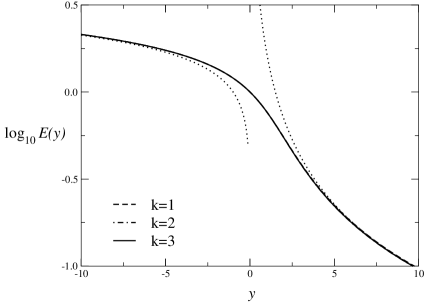
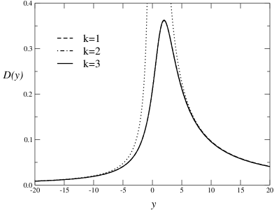
Figure 5: The scaling functions $E(y)$ and $D(y)$. We also plot their asymptotic behaviors (dotted lines): $E(y)\approx R_{\chi}y^{-\gamma}$ for $y\rightarrow+\infty$, and $E(y)\approx(-y)^{\beta}$ for $y\rightarrow-\infty$; $D(y)\approx R_{\chi}y^{-\gamma}$ for $y\rightarrow+\infty$, and $D(y)\approx\beta(-y)^{-\gamma}/f_{1}^{\rm coex}$ for $y\rightarrow-\infty$; Results from Ref. [243].

3.4.4 Trigonometric parametric representations

Refs. [426, 427, 428] considered the possibility of determining a parametric representation of the equation of state that also describes the two-phase region below the critical temperature. In the classical mean-field equation of state that describes a first-order transition, one finds a characteristic van der Waals (vdW) loop that represents an isothermal analytic continuation of the equation of state through the coexistence curve. For $t\to 0^{-}$, it has the simple cubic form $H\propto M(M^{2}-M_{0}^{2})$, which shows the classical critical exponents. The properties of the vdW loop are relevant for classical theories of surface tension, interfaces, spinodal decomposition, etc. (see, e.g., Refs. [961, 220]). In Refs. [426, 427, 428] the authors search for representations of the equation of state that, on the one hand, describe the nonclassical critical behavior of the system, and, on the other hand, have a good analytic continuation in the two-phase region. As also mentioned by the authors, the existence of a full vdW loop is not guaranteed in nonclassical theories, because of the presence of essential singularities at the coexistence curve [420, 402, 45, 560], which preclude the possibility of performing the required analytic continuation. Nevertheless, in Refs. [426, 427, 428] the classical thermodynamic picture was assumed and an analytic continuation of the critical equation of state was performed. They looked for parametric representations that give a reasonable realization of the vdW loop from their analytic continuation to the two-phase region. Polynomial representations do not offer a natural description of vdW loops. This is because the analytic continuation of these equations of state fails to generate a closed, continuous vdW loop inside the two-phase region. To overcome this problem, Ref. [426] proposed an interpolation scheme that ensured the expected vdW loop: The traditional parametric representations are retained, but a new angular variable $\phi$ is introduced to describe the two-phase region only, the values $\phi=\pm 1$ being assigned to the phase boundaries, while $\phi=0$ corresponds to the coexistence-curve diameter $M=0$, $H=0$. Thus, new angular functions describing the two-phase region are required, satisfying a matching condition that ensures the smoothness of the equation of state across the phase boundaries $H=0$, $t<0$. However, according to the authors, this procedure is not the optimal one. They noted that a natural description of the vdW loop requires analytic periodicity with period $2\theta_{p}$ with $\theta_{p}>\theta_{0}$. Therefore, they proposed an alternative approach based on trigonometric parametric representations:

$$M=m_{0}\,R^{\beta}\,m(\theta),\qquad t=R\,k(\theta),$$ (3.15)

$${\cal A}_{\rm sing}=n_{0}\,R^{2-\alpha}\,n(\theta),\qquad {\xi^{2}\over 2\chi}=R^{-\eta\nu}\,a(\theta),$$

where the traditional expression for $H$ is replaced by a direct parametrization of the singular part of the free energy ${\cal A}_{\rm sing}$. The parametric functions $m(\theta)$, $k(\theta)$, $n(\theta)$, and $a(\theta)$ are chosen to guarantee a closed analytic vdW loop:

$$m(\theta)={\sin(q\theta)\over q},\qquad k(\theta)=\left[1-{2b^{2}\over q^{2}}\left(1-\cos(q\theta)\right)\right],\qquad n(\theta)=1+\sum_{i=1}^{j}c_{i}k(\theta)^{i},$$

$$a(\theta)=a_{0}\left[1+{2a_{2}\over q^{2}}\left(1-\cos(q\theta)\right)+{a_{4}\over q^{4}}\left(1-\cos(q\theta)\right)^{2}\right],$$ (3.16)

where $q,b,c_{i},a_{i}$ are parameters that are determined by using known universal amplitude ratios. As shown in Ref. [428], this parametrization is able to provide a good fit to the universal amplitude ratios and reasonable vdW loops. They found that the shape of the vdW loop for three-dimensional Ising systems near criticality differs significantly from the classical form. In particular, the spinodal should be closer to the coexistence curve and the size of the vdW loop is smaller by approximately a factor of two.

3.4.5 Universal amplitude ratios

In this section we report the estimates of several universal amplitude ratios, see Table 2 for definitions. Those involving only zero-momentum quantities, such as the specific heat and the magnetic susceptibility, can be derived from the equation of state. Estimates of universal ratios involving correlation-length amplitudes, such as $Q^{+}$, $R_{\xi}^{+}$, and $Q_{c}$, can be obtained using the estimate of $g_{4}^{+}$. For instance, $Q^{+}=R_{4}^{+}R_{c}^{+}/g_{4}^{+}$. Other universal ratios can be derived by supplementing the above-reported results with the estimates of $w^{2}$ and $Q^{-}_{\xi}$ (which may be estimated by analyzing the corresponding LT expansions [240, 904, 58, 1081]) and the estimate of $Q^{+}_{\xi}$ (see Sec. 3.6 and Table 17). Moreover, in Ref. [240] estimate of $Q_{\xi}^{c}$ and $Q_{2}$ were obtained from approximate parametric representations of the correlation lengths $\xi$ and $\xi_{\rm gap}$, such as

$$a(\theta)=a(0)\left(1+c\theta^{2}\right),\qquad a_{\rm gap}(\theta)=a_{\rm gap}(0)\left(1+c_{\rm gap}\theta^{2}\right),$$ (3.17)

where $c$ and $c_{\rm gap}$ were obtained using the IHT estimates of $U_{\xi}$ and $U_{\xi_{\rm gap}}$.

In Table 11 we report the results obtained using the parametric representations reported in Sec. 3.4.3 (IHT-PR), from the analysis of HT and LT expansions (HT,LT), and from MC simulations. The results for $U_{2}$ and $U_{\xi}$ of Ref. [216] were obtained by taking $\beta_{c}$ and $\Delta$ as external inputs; the reported errors do not take into account the uncertainties on $\beta_{c}$ and $\Delta$, which should not be negligible. The IHT-PR estimates agree nicely with the most recent MC results, especially with those reported in Ref. [272], which are quite precise. There is a discrepancy only for $U_{0}$: The estimates reported in Ref. [518] are slightly larger. On the other hand, there is good agreement with the rather precise experimental result of Ref. [857]. It is worth mentioning that the result of Ref. [374] for $U_{2}$ was obtained by simulating a four-dimensional $SU(2)$ lattice gauge model at finite temperature.

Table 11 also reports some experimental results for binary mixtures, liquid-vapor transitions, and uniaxial antiferromagnetic systems. They should give an overview of the level of precision reached by experiments. Some of the experimental data are taken from Ref. [932]. Sometimes, we report a range of values without a corresponding reference: this roughly summarizes the results reported in the corresponding table of Ref. [932] and should give an idea of the range of the experimental results.

Table 12 shows the results obtained by FT methods. FT estimates are consistent, although in general less precise. We mention that the results denoted by “$d=3$ exp” were obtained using different schemes, see Sec. 2.4: the traditional zero-momentum scheme [79, 71], the minimal subtraction without $\epsilon$ expansion [686, 984], and the expansion in the LT coupling $u\equiv 3w^{2}$ [484]. Refs. [480, 481] used the fixed-dimension expansion and the $\epsilon$ expansion to determine the universal coefficients $r_{6}$, $r_{8}$, and $r_{10}$, which were then used to obtain an approximate parametric representation of the critical equation of state. The corresponding amplitude ratios are denoted by FT-PR.

Table 11: Estimates of universal quantities, see Table 2 for definitions. The results are obtained by combining HT results and the parametric representation of the equation of state (IHT–PR), from the analysis of high- and low-temperature expansions (HT,LT), and from Monte Carlo simulations (MC). For the experimental results: ms denotes a magnetic system; bm a binary mixture; lv a liquid-vapor transition; mi a micellar system. Experimental estimates without reference are taken from Ref. [932].

	IHT–PR [243, 240]	HT,LT	MC	experiments
$U_{0}$	0.532(3)	0.523(9) [715]	0.560(10) [519]	0.536(5) bm [857]
		0.51 [107]	0.550(12) [519]	0.538(17) lv [1029]
			0.567(16) [519]	0.54(2) ms [121]
			0.45(7) [759]	0.55(6) ms [760]
				0.47–0.53 lv
				0.54–0.58 bm
				0.52–0.56 ms
$U_{2}$	4.76(2)	4.762(8) [216]	4.75(3) [272]	4.3(3) bm [1139]
		4.95(15) [715]	4.72(11) [374]	4.5–5.3 lv
		5.01 [1050]		4.9(5) ms [307]
				4.6(2) ms [122]
$U_{4}$	$-$9.0(2)	$-$9.0(3) [1151]
$R_{c}^{+}$	0.0567(3)	0.0581(10) [1151]		0.050(15) bm [1139]
				0.04–0.06 lv
$R_{c}^{-}$	0.02242(12)
$R_{4}^{+}$	7.81(2)	7.94(12) [427]
$R_{4}^{-}$	93.6(6)	107(13) [1151, 427]
$R_{\chi}$	1.660(4)	1.57(23) [1150, 427]		1.75(30) bm [1139]
				1.69(14) lv [825]
$w^{2}$		4.75(4) [904]	4.77(3) [272]
		4.71(5) [1151, 412]
$U_{\xi}$	1.956(7)	1.963(8) [216]	1.95(2) [272]	2.0(4) bm [501]
		1.96(1) [715]	2.06(1) [965]	1.9(2) bm [1139]
		1.96 [1050]		1.89(4) ms [122]
				1.93(10) ms [307]
$U_{\xi_{\rm gap}}$	1.896(10)
$Q^{+}$	0.01880(8)	0.01899(11) [217]	0.0193(10) [519]	0.023(4) lv [530]
		0.0202(9) [215]		0.0187(13) bm [857]
		0.01880(15) [715]		0.016(4) mi [705]
				0.018–0.022 bm
$Q^{-}$	0.00472(5)	0.00477(20) [427]	0.0463(17) [519]
$Q_{c}$	0.3315(10)	0.324(6) [427]	0.328(5) [272]	0.3–0.4 bm
				0.34(19) bm [1116]
				0.36(3) bm [577]
				0.29(4) bm [46]
				0.3–0.4 lv
$Q_{\xi}^{+}$	1.000200(3)	1.0001 [427]
$Q_{\xi}^{c}$	1.024(4)	1.007(3) [427]
$Q_{\xi}^{-}$		1.032(4) [240]	1.031(6) [278, 11]
		1.037(3) [427]
$Q_{2}$	1.195(10)	1.17(2) [1150, 427]		1.1(3) bm [1139]
$v_{3}$	6.050(13)	6.44(30) [427, 1151]
$v_{4}$	16.17(10)
$g_{3}^{-}$	13.19(6)	13.9(4) [1151]	13.6(5) [1070]
$g_{4}^{-}$	76.8(8)	85 [1151]	108(7) [1070]
$P_{m}$	1.2498(6)
$R_{p}$	1.9665(10)
$R_{\sigma}$			0.1040(8) [518]
			0.1056(19) [11]
			0.098(2) [1150]
$R_{\sigma}^{+}$			0.40(1) [513]	0.38(3)
			0.377(11) [1150, 427]	0.41(4) bm [757]
				0.33(6) mi [705]

In Tables 11 and 12 we also report the universal amplitude ratios $R_{\sigma}$ and $R_{\sigma}^{+}$ involving the surface-tension amplitude, see Table 2 for definitions.

Table 12: FT estimates of universal quantities, see Table 2 for definitions. We report results obtained in the $\epsilon$ expansion ($\epsilon$ exp), in the fixed-dimension expansion in $d=3$ in different schemes (see text) ($d=3$ exp), using a parametric equation of state and $d=3$ and $\epsilon$-expansion results ($d=3$ and $\epsilon$ FT–PR) [480, 481], and in the continuous RG approach (CRG).

	$\epsilon$ exp	$d=3$ exp	$d=3$ FT–PR [481]	$\epsilon$ FT–PR [481]	CRG
$U_{0}$	0.524(10) [847, 137]	0.540(11)[686]	0.537(19)	0.527(37)
		0.541(14) [79]
$U_{2}$	4.9 [847]	4.77(30) [79]	4.79(10)	4.73(16)	4.966 [997]
	4.8 [176, 25]	4.72(17) [484]			4.29 [133]
$U_{4}$			$-$9.1(6)	$-$8.6(1.5)
$R_{c}^{+}$			0.0574(20)	0.0569(35)
$R_{4}^{+}$			7.84	8.24(34)
$R_{\chi}$	1.67 [847, 137]	1.7 [79]	1.669(18)	1.648(36)	1.647 [997]
					1.61 [133]
$w^{2}$		4.73 [484]
$U_{\xi}$	1.91 [176]	2.013(28) [484]			2.027 [997]
		2.04(4) [819]			1.86 [133]
$Q^{+}$	0.0197 [138, 137]	0.01968(15) [71]
$Q_{c}$		0.331(9) [79]
$Q_{\xi}^{+}$	1.00016(2) [240]	1.00021(3) [239]
$Q_{2}$	1.13 [176]
$v_{3}$	5.99(5) [906]		6.08(6)	6.07(19)
$v_{4}$	15.8(1.4) [906]
$g_{3}^{-}$	13.06(12)[906]
$g_{4}^{-}$	75(7)[906]
$R_{\sigma}$	0.055 [174]	0.1065(9) [818]

3.5 The two-dimensional Ising universality class

3.5.1 General results

In two dimensions a wealth of exact results exists. Many exact results have been obtained for the simplest model belonging to this universality class, the spin-$1/2$ Ising model. For the square-lattice Ising model we mention: the exact expression of the free energy along the $H=0$ axis [863], the two-point correlation function for $H=0$ [1135], and the spontaneous magnetization on the coexistence curve [1088]. For a review, see, e.g., Ref. [777]. Moreover, in the critical limit several amplitudes are known to high precision, see, e.g., Refs. [841, 871]. Besides, at the critical point one can use conformal field theory. This provides the exact spectrum of the theory, i.e. all the dimensions of the operators present in the model. In particular, one finds [223, 277] that the first rotationally-invariant correction-to-scaling operator has dimension $y_{3}=-2$, i.e. $\omega=2$. Moreover, the exponent $\omega_{NR}$ that gives the corrections related to the breaking of the rotational invariance can be exactly predicted [239, 274, 223, 277]: $\omega_{NR}=2$ on the square lattice and $\omega_{NR}=4$ on the triangular lattice.

Table 13: Critical exponents and universal amplitude ratios for the two-dimensional Ising universality class, taken from Refs.[1135, 326, 240, 275, 223]. Since the specific heat diverges logarithmically, the specific-heat amplitudes $A^{\pm}$ are defined by $C_{H}\approx-A^{\pm}\log t$. See Sec. 1.3 for the definitions of the other amplitudes. The definition of $R^{\pm}_{c}$ and $Q^{\pm}$ differ from those given in Table 2 because of the absence of $\alpha$, which is zero in this case. The value of $\omega_{NR}$ depends on the lattice that is considered: The reported values refer to the square (sq) and triangular (tr) lattices respectively.

$\gamma$	7/4
$\nu$	1
$\eta$	1/4
$\beta$	1/8
$\delta$	15
$\omega$	2
$\omega_{NR}$	2 (sq),   4 (tr)
$U_{0}\equiv A^{+}/A^{-}$	1
$U_{2}\equiv C^{+}/C^{-}$	37.69365201
$R_{c}^{+}\equiv A^{+}C^{+}/B^{2}$	0.31856939
$R_{c}^{-}\equiv A^{-}C^{-}/B^{2}$	0.00845154
$R_{\chi}\equiv Q_{1}^{-\delta}\equiv C^{+}B^{\delta-1}/(B^{c})^{\delta}$	6.77828502
$w^{2}\equiv C^{-}/[B^{2}(f^{-})^{2}]$	0.53152607
$U_{\xi}\equiv f^{+}/f^{-}$	3.16249504
$U_{\xi_{\rm gap}}\equiv f^{+}_{\rm gap}/f^{-}_{\rm gap}$	2
$Q^{+}\equiv A^{+}(f^{+})^{2}$	0.15902704
$Q^{-}\equiv A^{-}(f^{-})^{2}$	0.015900517
$Q^{+}_{\xi}\equiv f^{+}_{\rm gap}/f^{+}$	1.000402074
$Q^{c}_{\xi}\equiv f^{c}_{\rm gap}/f^{c}$	1.0786828
$Q^{-}_{\xi}\equiv f^{-}_{\rm gap}/f^{-}$	1.581883299
$Q_{2}\equiv(f^{c}/f^{+})^{2-\eta}C^{+}/C^{c}$	2.8355305

Additional results have been obtained using the $S$-matrix approach to two-dimensional integrable theories and in particular the thermodynamic Bethe Ansatz (for a review, see, e.g., Ref. [777]). Indeed, the quantum field theories that describe the critical regime for $H=0$ and $t=0$ are integrable and one can compute the corresponding $S$-matrices. While for $H=0$ the $S$-matrix is trivial, for two-particle scattering $S=-1$, on the critical isotherm the $S$-matrix solution is complex with a nontrivial mass spectrum [1140]. A related method is the form-factor approach, which uses the knowledge of the $S$-matrix to set up a system of recursive functional equations for the form factors. By solving this system, one can in principle compute exactly all the form factors, thus performing an analytic continuation of the $S$-matrix off mass shell [607, 1017]. Once the form factors are known, one can compute the correlation functions of the fundamental field, as well as of other composite operators, by inserting complete sets of scattering states between them. This gives the correlation functions as infinite series of convolution products of form factors.

In Table 13 we report some exact results and some high-precision estimates of the amplitude ratios that have been obtained using the approaches that we mentioned above. In Table 14 we report estimates of the zero-momentum four-point coupling $g_{4}^{+}$, for which very precise estimates have been recently obtained by various methods.

Table 14: Estimates of $g_{4}^{+}$ for the two-dimensional Ising universality class. We report the existing results obtained using transfer-matrix techniques combined with RG scaling (TM+RG), the form-factor approach (FF), high-temperature expansions (HT), Monte Carlo simulations (MC), field theory (FT) based on the $\epsilon$ expansion and the fixed-dimension $d=2$ expansion, and a method based on a dimensional expansion around $d=0$ ($d$ exp).

Ref.	Method	$g_{4}^{+}$
[276, 275] 2000	TM+RG	14.697323(20)
[101] 2000	FF	14.6975(1)
[904] 1998	HT	14.694(2)
[211] 1996	HT	14.693(4)
[1151] 1996	HT	14.700(17)
[101] 2000	MC	14.69(2)
[638] 2000	MC	14.7(2)
[907] 2000	FT $\epsilon$ exp	14.7(4)
[870] 2000	FT $d=2$ exp	15.4(3)
[693] 1977	FT $d=2$ exp	15.5(8)
[127] 1992	$d$ exp	14.88(17)

The two-dimensional Ising universality class is also of experimental interest. Indeed, there exist several uniaxial antiferromagnets which present a strongly enhanced in-plane coupling and an easy-axis anisotropy (see, e.g., Refs. [932, 529, 1137] for some experimental results), and have therefore a two-dimensional Ising critical behavior. Ising behavior has also been observed in several order-disorder and structural transitions: in monolayers of carbon monoxide and C₂F₆ physisorbed on graphite [382, 1118, 59], in adsorbed hydrogen on Ni [204], and in GaAs(001) surfaces [681]. We also mention an experimental study of the Yang-Lee edge singularities in FeCl₂ [152].

3.5.2 The critical equation of state: exact results

The behavior of the free energy for the two-dimensional Ising model is somewhat different from that described in Sec. 1.5. The reason is that in this case there are resonances among the RG eigenvalues with the subsequent appearance of logarithmic terms. Because of the resonance between the identity and the thermal operator, the singular part of the Gibbs free energy becomes [1105]

$${\cal F}_{\rm sing}(H,t)=t^{2}\widehat{\cal F}_{1}(Ht^{-15/8})+t^{2}\log|t|\,\widehat{\cal F}_{1,\rm log}(Ht^{-15/8}),$$ (3.18)

where irrelevant terms have been discarded. Note that additional resonances involving subleading operators are expected, and thus additional logarithmic terms should be present: such terms, involving higher powers of $\log|t|$, have been found in a high-precision analysis of the susceptibility for $H=0$ in the HT phase [871]. The exact results for the free energy at $H=0$ and the numerical results for the higher-order correlation functions at zero momentum show that $\widehat{\cal F}_{1,\rm log}(x)$ is constant [23]. Indeed, if this function were nontrivial, then one would obtain $\chi_{n}\sim|t|^{-\gamma_{n}}\log|t|$ for $|t|\to 0$, a behavior that has not been observed. The constant is easily related to the amplitudes of the specific heat for $H\to 0$ defined in Eq. (1.43). The analyticity for $t=0$, $H\not=0$ implies

$$A^{+}=A^{-}\equiv A,$$ (3.19)

so that

$${\cal F}_{\rm sing}(H,t)=t^{2}\widehat{\cal F}_{1}(Ht^{-15/8})+{A\over 2}t^{2}\log|t|.$$ (3.20)

For the Helmholtz free energy similar formulae holds. Using the notations of Sec. 1.5.2 we write

$${\cal A}_{\rm sing}(M,t)=a_{11}t^{2}A_{1}(z)+{A\over 2}t^{2}\log|t|=a_{20}M^{16}A_{2}(x)+{A\over 2}t^{2}\log|t|,$$ (3.21)

where $a_{11}$ and $a_{20}$ are defined in Eqs. (1.65) and (1.68), the variables $z$ and $x$ in Eqs. (1.62) and (1.66), and the functions $A_{1}(z)$ and $A_{2}(x)$ are normalized as in Sec. 1.5.2. The presence of the logarithmic term gives rise to logarithms in the expansions of $A_{1}(z)$ for $z\to\infty$ and $A_{2}(x)$ for $x\to 0$. Indeed, the analyticity of ${\cal A}_{\rm sing}(M,t)$ for $t=0$, $|M|\not=0$ implies

$$A_{1}(z) = z^{16}\sum_{n=0}a_{1,n}z^{-8n}+a_{1,\rm log}\log z,$$ (3.22)

$$A_{2}(x) = \sum_{n=0}a_{2,n}x^{n}+a_{2,\rm log}x^{2}\log|x|.$$ (3.23)

The constant $a_{1,\rm log}$ and $a_{2,\rm log}$ are easily expressed in terms of invariant amplitude ratios:

$$a_{1,\rm log}={4A\over a_{11}}=4Q^{+}g_{4}^{+},\qquad a_{2,\rm log}=-{A\over 2a_{20}B^{16}}=-{8R^{+}_{c}\over R_{\chi}}.$$ (3.24)

For the equation of state we have

$${H}={\partial{\cal A}\over\partial{M}}=a_{11}b_{1}t^{15/8}F(z)=(B^{c})^{-15}M^{15}f(x),$$ (3.25)

where $F(z)$ and $f(x)$ are defined in Eq. (1.71). The properties of these two functions are described in Sec. 1.5.3. Using Eqs. (3.22) and (3.23) we can compute the coefficients $F_{2}^{\infty}$ and $f_{2}^{0}$ appearing in the expansions of $F(z)$ and of $f(x)$ for $z\to\infty$ and $x\to 0$ respectively, cf. Eqs. (1.82) and (1.88). We have $F_{2}^{\infty}=a_{1,\rm log}$ and $f^{0}_{2}=-{\textstyle\frac{1}{2}}a_{2,\rm log}$.

A detailed study of the analytic properties of the critical equation of state can be found in Ref. [439].

3.5.3 Approximate representations of the equation of state

The equation of state in the whole $(t,H)$ plane is not known exactly, only approximate results are available. Approximate parametric representations have been determined in Ref. [276], using the variational approach presented in Sec. 3.4.2. Specifically, the parametrization (3.7) was used, and the $k$ parameters $h_{3},\ldots,h_{2k+1}$ were determined by requiring the approximate representation to reproduce the $(k-2)$ invariant ratios $r_{2n}$, $n:3,\ldots,k$, and the large-$z$ behavior of the function $F(z)$, $F(z)\approx F_{0}^{\infty}z^{\delta}$, and to satisfy the global stationarity condition (3.11); see Sec. 3.4.2 for details of the method.

In order to apply the method, good estimates of the coefficients $r_{2n}$, which parametrize the small-magnetization expansion of the Helmholtz free energy, and of $F_{0}^{\infty}$ are needed. The latter constant can be obtained from the results of Table 13 and the precise estimate of $g_{4}^{+}$ of Ref. [276] reported in Table 14. Indeed,

$$R_{4}^{+}\equiv{g_{4}^{+}Q^{+}\over R^{+}_{c}}=7.336774(10),\qquad F_{0}^{\infty}=R_{\chi}(R^{+}_{4})^{(1-\delta)/2}=5.92357(6)\times 10^{-5}.$$ (3.26)

Accurate estimates of the first coefficients $r_{2n}$, see Table 15, have been recently determined in Refs. [276, 241], using transfer-matrix techniques and general RG properties. Another approach is presented in Ref. [439], where the authors exploit the analytic properties of the free energy to write down a dispersion relation. Approximate expressions for the corresponding kernel are obtained using the knowledge of the behavior of the free energy at the Yang-Lee edge singularity [408, 264]. The estimates of first few $r_{2n}$ obtained in this approach, see Table 15, are in good agreement with the results of Ref. [276]. The comparison worsens for the higher-order coefficients, showing the limitations of the approximation employed. The coefficients appearing in the expansion of the scaling function $Q(u)$ around $u=1$, cf. Eq. (1.94), have also been determined. We report the results [906] $v_{3}=33.011(6)$, $v_{4}=48.6(1.2)$ from LT expansions and [439] $v_{3}=33.0502$, $v_{4}=48.0762$ from an appropriate dispersion relation. Estimates of $v_{n}$ for $n>4$ are reported in Ref. [906] and can also be derived from the results of Ref. [439].

Table 15: Estimates of the coefficients $r_{2n}$. They have been determined by transfer-matrix techniques supplemented with RG results (TM+RG) [276], using approximate parametric representations of the equation of state (TM+RG+PR) [276], and by means of a dispersive approach (Disp) [439].

	TM+RG [276]	TM+RG+PR [276]	Disp [439]
$r_{6}$	3.67867(7)		3.67797
$r_{8}$	26.041(11)		26.0332
$r_{10}$	284.5(2.4)		286.12
$r_{12}$	$4.2(7)\times 10^{3}$	$4.44(6)\times 10^{3}$	4215
$r_{14}$		$8.43(3)\times 10^{4}$	$-$7356

Finally, we present the results of Ref. [276] for the equation of state. In Table 16, for $k=2,3,4,5$, we report the polynomials $h(\theta)$ obtained using the global stationarity condition (3.11) and the central values of the input parameters $F^{\infty}_{0}$, $r_{6}$, $r_{8}$, $r_{10}$. In Fig. 6 we show the scaling functions $f(x)$ and $F(z)$, as obtained from ${h}(\theta)$ for $k=2,3,4,5$. The convergence is satisfactory. The scaling function $F(z)$ is determined with a relative uncertainty of at most a few per thousand in the whole region $z\geq 0$. The convergence is slower at the coexistence curve, so that the error on the fuction $f(x)$ is of a few per cent.

Table 16: Polynomial approximations of $h(\theta)$ obtained using the variational approach for several values of the parameter $k$, cf. Eq. (3.7). The reported expressions correspond to the central values of the input parameters. Results from Ref. [276].

$k$	$\theta_{0}^{2}$	${h}(\theta)/[\theta(1-\theta^{2}/\theta_{0}^{2})]$
2	1.15278	$1-0.208408\theta^{2}$
3	1.15940	$1-0.215675\theta^{2}-0.039403\theta^{4}$
4	1.16441	$1-0.219388\theta^{2}-0.041791\theta^{4}-0.013488\theta^{6}$
5	1.16951	$1-0.222389\theta^{2}-0.043547\theta^{4}-0.014809\theta^{6}-0.007168\theta^{8}$

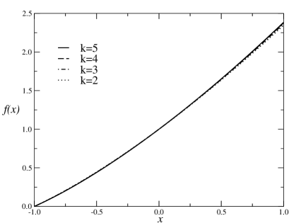
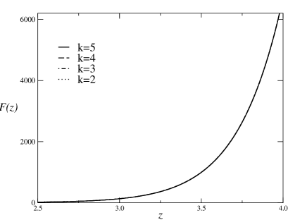
Figure 6: The scaling functions $f(x)$ and $F(z)$ as obtained from the polynomial approximations (3.7) for $k=2,3,4,5$. Results from Ref. [276].

3.6 The two-point function of the order parameter

We shall discuss here the two-point function of the order parameter, that is relevant in the description of scattering phenomena, see Sec. 3.6.3. We mention that also the energy-energy correlation function has been computed [833, 227]. It is relevant in the description of elastic deformations in fluids and it can be measured via sound-attenuation techniques [833].

We shall concentrate on the experimentally relevant case $H=0$. Results on the whole $(t,H)$ plane and on the critical isotherm can be found in Refs. [1050, 300]. For the two-dimensional case we mention that the large-distance expansion of the two-point function on the critical isotherm, i.e. for $t=0$ and $H\neq 0$, has been determined using the form-factor approach in Refs. [327, 328].

3.6.1 High-temperature phase

As discussed in Sec. 1.6.1, the two-point correlation function $\widetilde{G}(q)$ has the scaling form (1.126). For $y\equiv q^{2}\xi^{2}\to 0$, the function $g^{+}(y)$ has the expansion (1.128). In Table 17 we report the estimates of the first few coefficients $c_{n}^{+}$, obtained from the analysis of HT expansions, from the FT fixed-dimension expansion, and from the $\epsilon$ expansion. There, we also report the invariant ratios $S_{M}^{+}$ and $S_{Z}^{+}$, see Eq. (1.131), that parametrize the large-distance behavior of $G(x)$.

Table 17: Estimates of $c_{i}^{+}$, $S_{M}^{+}$, and $S_{Z}^{+}$ for the three-dimensional Ising universality class. Note $Q^{+}_{\xi}=\left(S_{M}^{+}\right)^{-1/2}$.

	HT	$\epsilon$ exp	$d=3$ exp
$c_{2}^{+}$	$-$3.90(6)$\times 10^{-4}$ [243]	$-$3.3(2) $\times 10^{-4}$ [240]	$-$4.0(5) $\times 10^{-4}$ [239]
	$-$3.0(2)$\times 10^{-4}$ [239]
	$-$5.5(1.5)$\times 10^{-4}$, $-$7.1(1.5)$\times 10^{-4}$ [1050]
$c_{3}^{+}$	0.882(6)$\times 10^{-5}$ [243]	0.7(1) $\times 10^{-5}$ [240]	1.3(3) $\times 10^{-5}$ [239]
	1.0(1)$\times 10^{-5}$ [239]
	0.5(2)$\times 10^{-5}$, 0.9(3)$\times 10^{-5}$ [1050]
$c_{4}^{+}$	$-0.4(1)\times 10^{-6}$ [243]	$-$0.3(1)$\times 10^{-6}$ [240]	$-$0.6(2)$\times 10^{-6}$[239]
$S_{M}^{+}$	0.999601(6) [243]	0.99968(4) [240]	0.99959(6) [239]
	0.99975(10) [239]
$S_{Z}^{+}$	1.000810(13)[243]

The coefficients $c_{n}^{+}$ show the pattern

$$|c_{n}^{+}|\ll|c_{n-1}^{+}|\ll...\ll|c_{2}^{+}|\ll 1$$ (3.27)

for $n\geq 3$. This is in agreement with the theoretical expectation that the singularity of $g^{+}(y)$ nearest to the origin is the three-particle cut [393, 172]. If this is the case, the convergence radius $r_{g}$ of the Taylor expansion of $g^{+}(y)$ is $r_{g}=9S_{M}^{+}$. Since $S_{M}^{+}\approx 1$, at least asymptotically we should have

$$c_{n+1}^{+}\approx-{1\over 9}c_{n}^{+}.$$ (3.28)

This behavior was checked explicitly in the large-$N$ limit of the $N$-vector model [239]. In two dimensions, the critical two-point function can be written in terms of the solutions of a Painlevé differential equation [1135] and it can be verified explicitly that $r_{g}=9S_{M}^{+}$. In Table 18 we report the values of $c_{i}^{+}$ for the two-dimensional Ising model. They are taken from Refs. [1067, 240].

For large $y$ the function $g^{+}(y)$ follows the Fisher-Langer law (1.129). The coefficients $A^{+}_{n}$ have been computed to three loops in Ref. [172]. In three dimensions one obtains the estimates $A_{1}^{+}\approx 0.92$, $A_{2}^{+}\approx 1.8$, and $A_{3}^{+}\approx-2.7$. In two dimensions the Fisher-Langer law must be modified since $\alpha=0$. In this case, for large values of $y$, $g^{+}(y)$ behaves as

$$g^{+}(y)^{-1}\approx{A^{+}_{1}\over y^{7/8}}\left(1+{A^{+}_{2}\over y^{1/2}}\,\log y+{A^{+}_{3}\over y^{1/2}}\right),$$ (3.29)

where the coefficients are [1067] $A_{1}^{+}\approx 0.413840$, $A_{2}^{+}\approx 0.802998$, and $A_{3}^{+}\approx 0.395345$.

In the years, several parametrizations of the scaling function $g^{+}(y)$ have been proposed, see, e.g., Refs. [418, 1050, 1067, 172]. The most successful approximation is the one proposed by Bray [172]. It is based on a dispersive approach [393, 392] and, by definition, it has the correct large-$y$ behavior (1.129) and has the pattern (3.28) built in. In this approach one fixes the values of the exponents and of the sum $A_{2}^{+}+A_{3}^{+}$ and determines an approximation of $g^{+}(y)$. The accuracy of the results can be evaluated by comparing the predictions for $c^{+}_{n}$ and for the coefficients $A_{i}^{+}$ with those obtained above. Using Bray’s parametrization one obtains $A_{1}^{+}\approx 0.918$, $A_{2}^{+}\approx 2.55$, $A_{3}^{+}\approx-3.45$, $c_{2}^{+}\approx-4.2\times 10^{-4}$, and $c_{3}^{+}\approx 1.0\times 10^{-5}$. These estimates are in reasonable agreement with those reported in Table 17 and with the $\epsilon$-expansion results for $A^{+}_{n}$.

Bray’s approach was also applied in two dimensions. A slightly different approximation that makes use of the high-precision results for $A_{1}^{+}$, $A_{2}^{+}$, and $A_{3}^{+}$ reproduces the results of Ref. [1067] with a maximum error of 0.03%.

Table 18: Values of $c_{i}^{\pm}$ and $S_{M}^{\pm}$ for the two-dimensional Ising universality class. Results from Refs. [1067, 240].

HT phase	LT phase
$S_{M}^{+}=0.999196337056$	$S_{M}^{-}=0.399623590999$
$c_{2}^{+}=-0.7936796064\times 10^{-3}$	$c_{2}^{-}=-0.42989191603$
$c_{3}^{+}=0.109599108\times 10^{-4}$	$c_{3}^{-}=0.5256121845$
$c_{4}^{+}=-0.3127446\times 10^{-6}$	$c_{4}^{-}=-0.8154613925$
$c_{5}^{+}=0.126670\times 10^{-7}$	$c_{5}^{-}=1.422603449$
$c_{6}^{+}=-0.62997\times 10^{-9}$	$c_{6}^{-}=-2.663354573$

The three-dimensional correlation function was studied in Ref. [767] by means of a MC simulation. The function $g^{+}(y)$ was determined with 0.5% (resp. 1%) precision up to $q\xi\approx 5$ (resp. 30). The numerical results were used to determine an interpolation that reproduces the MC results for $y$ small and has the Fisher-Langer behavior (1.129) behavior for $y\to\infty$.

3.6.2 Low-temperature phase

In the LT phase, one introduces a scaling function $g^{-}(y)$ that is defined as $g^{+}(y)$ in Eq. (1.126). For $y\to 0$, also $g^{-}(y)$ admits a regular expansion of the form (1.128) with different coefficients $c_{n}^{-}$. With respect to the HT case, for $y$ small the deviations from the Gaussian (Ornstein-Zernike) behavior are larger. From the $\epsilon$ expansion at two loops, Ref. [300] obtains $c_{2}^{-}\approx-2.4\times 10^{-2}$ and $c_{3}^{-}\approx 3.9\times 10^{-3}$, in reasonable agreement with the series estimates of Ref. [1050]: $c_{2}^{-}\approx-1.2(6)\times 10^{-2}$ and $c_{3}^{-}\approx 7(3)\times 10^{-3}$. The larger deviations from the Gaussian behavior are confirmed by the estimates of $S_{M}^{-}$: $S_{M}^{-}=0.938(8)$ [240] and $S_{M}^{-}=0.930(6)$ [427] from the analysis of the LT expansion, and $S_{M}^{-}=0.941(11)$ [278, 11] from MC simulations. Such a different behavior is probably related to the different analytic structure of the two-point function in the LT phase. Indeed, perturbative arguments indicate the presence of a two-particle cut in the LT phase [300, 393, 172]. Thus, the convergence radius of the small-$y$ expansion is expected to be at most $4S_{M}^{-}$, and asymptotically $c_{n+1}^{-}\approx-0.27\,c_{n}^{-}$. For large values of $y$, $g^{-}(y)$ follows the Fisher-Langer law (1.129) with different coefficients $A_{n}^{-}$. They can be derived from $A_{n}^{+}$ using Eq. (1.133). These relations have been checked in Ref. [300] to two-loop order in the $\epsilon$ expansion.

The mass spectrum of the model in the LT phase was investigated in Refs. [278, 11, 933, 279] using numerical techniques. In particular, Ref. [278] reports MC results obtained from simulations of the standard Ising model and of the improved $\phi^{4}$ lattice model (1.7) at $\lambda=1.10$ (see Sec. 2.3.2), and provides evidence for a state with $M_{2}<2M$, where $M$ is the mass of the fundamental state, i.e. ${M_{2}/M}=1.83(3)$, that is below the pair-production threshold. This second state should appear as a pole in the Fourier transform of the two-point function.

The two-dimensional Ising model shows even larger deviations from Eq. (1.127), as one can see from the estimates of $S_{M}^{-}$ and $c_{i}^{-}$ reported in Table 18. Note that in the LT phase of the two-dimensional Ising model the singularity at $k^{2}=-1/\xi^{2}_{\rm gap}$ of $\widetilde{G}(k)$ is not a simple pole, but a branch point [1135]. As a consequence, the convergence radius of the expansion around $y=0$ is $S_{M}^{-}$.

For large values of $y$, $g^{-}(y)$ behaves according to Eq. (3.29), with different coefficients $A_{n}^{-}$. They are given by [1067]: $A_{1}^{-}\approx 2.07993$, $A_{2}^{-}\approx-0.253913$, and $A_{3}^{-}\approx-0.709701$. Bray’s approximation has been also applied to the LT phase, see Ref. [767].

3.6.3 Experimental results

In scattering experiments one measures the scattering cross-section

$${d^{2}\sigma\over dqd\omega}$$ (3.30)

where $q$ is the exchanged momentum vector and $\omega$ the corresponding frequency (energy). This cross-section is proportional to the dynamic structure factor $S(q,\omega)$. In the critical limit, $S(q,\omega)$ is dominated by the elastic Rayleigh peak, whose width goes to zero as $t\to 0$. Thus, in this limit only elastic scattering is relevant and

$${d\sigma\over dq}\propto\int d\omega S(q,\omega)=\widetilde{G}(q).$$ (3.31)

The momentum-transfer vector $q$ is related to the scattering angle $\theta$ by

$$q={4\pi\over\lambda}\sin{\theta\over 2},$$ (3.32)

where $\lambda$ is the wavelength of the radiation (neutrons) in the scattering medium. Note that scattering data can be directly related to $\widetilde{G}(q)$ only if multiple scattering can be neglected. See Ref. [49] for a discussion.

Several experiments determined the scaling functions $g^{\pm}(y)$ in magnetic systems [118] and in fluids. In the HT phase, because of the smallness of the coefficients $c^{+}_{n}$, the Ornstein-Zernike approximation $g^{+}(y)\approx 1+y$ can be used up to $y\approx 30$. For larger values of $y$ it is necessary to take into account the anomalous behavior [141, 284, 987, 313, 575, 586, 978, 696, 164, 165, 314, 167, 166]. The large-momentum behavior of $g^{+}(y)$ has been extensively studied. In particular, the exponent $\eta$ and the constant $A_{1}^{+}$ have been determined: $\eta=0.017(15)$, $A_{1}^{+}=0.96(4)$ and $\eta\approx 0.030(25)$, $A_{1}^{+}\approx 0.95(4)$ (two different parametrizations of the structure factor are used) [284]; $\eta=0.0300(15)$, $A_{1}^{+}\approx 0.92(1)$ [313]; $\eta=0.042(6)$, $A_{1}^{+}\approx 0.915(21)$ [314]. No unbiased determination of $A_{2}^{+}$ and $A_{3}^{+}$ is available. Fixing $A_{2}^{+}+A_{3}^{+}=-0.9$ (the $\epsilon$-expansion result of Ref. [172]), Ref. [314] obtains $A_{2}^{+}=2.05(80)$ and $A_{3}^{+}=-2.95(80)$, in reasonable agreement with the $\epsilon$-expansion predictions.

A very precise determination of $g^{+}(y)$ was obtained in Ref. [314]. From the analysis of scattering data for CO₂, the function $g^{+}(y)$ was determined up to $y=1600$. These experimental results are in good agreement with the theoretical determinations (within an accuracy of approximately 1%).

3.6.4 Turbidity

The turbidity $\tau$ is defined as the attenuation of the transmitted light intensity per unit optical path length due to the scattering with the sample. Explicitly, it is given by

$$\tau\sim\int d\Omega\,\widetilde{G}(q)\sin^{2}\Phi,$$ (3.33)

where $\Omega$ is the scattering solid angle, $q$ is given by Eq. (3.32), and $\Phi$ is the angle between the polarization of the incoming radiation (or neutrons) and the scattering wave vector.

If $k_{0}=2\pi n/\lambda$ is the momentum of the incoming radiation in the medium, $\lambda$ the corresponding wavelength in vacuum, $n$ the refractive index, for small $k_{0}\xi$ the Puglielli-Ford expression [935] can be used:

$$\tau_{\rm PF}=\tau_{0}t^{-\gamma}\left[{2a^{2}+2a+1\over a^{3}}\log(2a+1)-{2(a+1)\over a^{2}}\right],$$ (3.34)

where $a=2k_{0}^{2}\xi^{2}$ and $\tau_{0}$ is a temperature-independent constant. Deviations are less than 1% (resp. 3%) for $k_{0}\xi\mathrel{\hbox to0.0pt{\lower 3.0pt\hbox{$\mathchar 536\relax$}\hss}\raise 2.0pt\hbox{$\mathchar 316\relax$}}15$ (resp. 90). An extensive discussion of the deviations from the Puglielli-Ford expression is given in Ref. [767]. In particular, in the experimentally relevant interval $k_{0}\xi\mathrel{\hbox to0.0pt{\lower 3.0pt\hbox{$\mathchar 536\relax$}\hss}\raise 2.0pt\hbox{$\mathchar 316\relax$}}100$, the turbidity can be computed using the expression [767]

$$\tau=\tau_{\rm PF}\left[0.666421+0.242399\left(1+0.0087936Q_{0}^{2}\right)^{0.018195}+0.0911801\left(1+0.09Q_{0}^{4}\right)^{0.0090975}\right],$$ (3.35)

where $Q_{0}\equiv k_{0}\xi$. Other results for the turbidity can be found in Refs. [391, 231]. However, as discussed in Ref. [767], they predict a turbidity that is larger than Eq. (3.35), which is based on the most accurate approximations of the structure factor available today.

The turbidity $\tau$ is larger than $\tau_{\rm PF}$ since $g^{+}(y)$ increases slower for $y\to\infty$ than the Ornstein-Zernike approximation. However, this is apparently in contrast with the experimental results for the binary fluid mixture methanol-cyclohexane presented in Ref. [578].

4 The three-dimensional $XY$ universality class

4.1 Physical relevance

The three-dimensional $XY$ universality class is characterized by a two-component order parameter and effective short-range interactions with U(1) symmetry. The most interesting representative of this universality class is the superfluid transition of ⁴He along the $\lambda$-line $T_{\lambda}(P)$. It provides an exceptional opportunity for a very accurate experimental test of the RG predictions, because of the weakness of the singularity in the compressibility of the fluid, of the purity of the samples, and of the possibility of performing experiments in a microgravity environment, for instance on the Space Shuttle as the experiment reported in Ref. [708], thereby achieving a significant reduction of the gravity-induced broadening of the transition. Exploiting these favorable conditions, the specific heat of liquid helium was measured to within a few nK from the $\lambda$-transition [708], i.e. very deep in the critical region, where the scaling corrections are small. Ref. [708] obtained the very precise estimate $\alpha=-0.01056(38)$. This result represents a challenge for theorists. Only recently have the theoretical estimates reached a comparable accuracy.

Beside ⁴He, there are many other systems that undergo an $XY$ transition. First of all, one should mention ferromagnets or antiferromagnets with easy-plane anisotropy, which is the original characterization of the $XY$ universality class.

An $XY$ behavior is observed in systems that exhibit phase transitions characterized by the establishement of a density wave. Indeed, the order parameter of density waves in a uniaxial system is the complex amplitude $\phi_{1}$, associated with the contribution ${\rm Re}\,\phi_{1}e^{iq_{0}z}$ to the density modulation, where $q_{0}$ is the wavelength of the modulation. Interesting examples in solids are charge-density wave (see, e.g., Refs. [430, 461]) and spin-density wave systems (see, e.g., Ref. [380]). Similar phenomena occur in liquid crystals, in which several transitions are expected to belong to the $XY$ universality class [324, 830, 200, 714, 49, 1008]. We should mention the nematic–smectic-A phase transition, that corresponds to the establishement of a one-dimensional mass-density wave along the direction of the orientational order, although experiments have found a wide range of effective exponents that are often quite different from the $XY$ predictions, see Refs. [449, 448] and references therein. The smectic-A–hexatic-B transition should by either $XY$ or first-order [20]; again experimental results are contradictory, see Ref. [679] and references therein. The same behavior is expected for the smectic-A–smectic-C and the smectic-A–chiral-smectic-C transitions [324]; in this case it is found experimentally that the $XY$ window is very small and one usually observes a crossover from mean-field to $XY$ critical behavior, see, e.g., Refs. [368, 367] and references therein. Finally, we should mention the nematic-to-lamellar phase transition, which is similar to the nematic–smectic-A transition [1004].

$XY$ criticality is expected in materials that undergo a phase transition from a normal (disordered) HT phase to a LT incommensurate modulated phase in one direction [306]. Such a transition is expected in some rare-earth metals like Er and Tm that are longitudinally modulated. The experimental evidence is however quite controversial, see Refs. [493, 706, 534]. A similar transition is observed in some insulating crystals of type A₂BX₄ [311], where $A^{+}$ is a monovalent cation like K⁺ or Rb⁺, and BX${}_{4}^{--}$ is a divalent tetrahedral anion like ZnCl${}_{4}^{--}$ or ZnBr${}_{4}^{--}$.

The $XY$ model is relevant for superconductors, as long as one is able to neglect the fluctuations of the magnetic potential. We mention that an inverted $XY$-scaling scenario is invoked in the description of superconductors in the extreme type-II region, where the transition is expected to be of second order, see, e.g., Ref. [792]. The idea is to use duality arguments to map the Ginzburg-Landau model with a U(1) gauge field with temperature parameter $\tau$ into an XY model with inverted temperature $-\tau$ [316, 647]. High-temperature superconductors for small magnetic fields are also found to show $XY$ behavior [1005] (for a different point of view, see Refs. [960, 598, 303]), both for the statics and the dynamics, see, e.g., Refs. [872, 68, 677, 643, 824, 505, 954, 953] and references therein.

The Peierls transition in CuGeO₃ and in some organic materials has been identified with an $XY$ transition. Indeed, the latest intensity measurements give estimates of $\beta$ that are in good agreement with the theoretical predictions, see Refs. [737, 736] and references therein. On the other hand, scattering experiments either do not observe critical scattering or observe anomalous line shapes with exponents $\gamma$ and $\nu$ much larger than expected, see, e.g., Refs. [510, 736] and references therein.

4.2 The critical exponents

4.2.1 Theoretical results

In Table 19 we report the theoretical estimates of the critical exponents.

Table 19: Estimates of the critical exponents for the three-dimensional $XY$ universality class. We indicate with an asterisk (^∗) the estimates we obtained using the hyperscaling relation $2-\alpha=3\nu$ or the scaling relation $\gamma=(2-\eta)\nu$. When the error was not reported by the authors, we used the independent-error formula to estimate it.

Ref.		info	$\gamma$	$\nu$	$\eta$	$\alpha$	$\omega$
[233]	2001	MC+IHT, $\phi^{4}$, dd$XY$	1.3177(5)	0.67155(27)	0.0380(4)	$-$0.0146(8)∗
[241]	2000	IHT, $\phi^{4}$	1.3179(11)	0.67166(55)	0.0381(3)	$-$0.0150(17)∗
[215]	1999	HT, $XY$ sc		0.671(3)∗		$-$0.014(9)
[215]	1999	HT, $XY$ bcc		0.674(2)∗		$-$0.022(6)
[213]	1997	HT, $XY$ sc	1.325(3)	0.675(2)	0.037(7)∗	$-$0.025(6)∗
[213]	1997	HT, $XY$ bcc	1.322(3)	0.674(2)	0.039(7)∗	$-$0.022(6)∗
[219]	1993	HT, $XY$ sc	1.315(9)	0.68(1)	0.07(3)∗	$-$0.04(3)∗
[385]	1973	HT $XY$, easy-plane	1.318(10)	0.670(6)	0.04(1)∗	$-$0.02(3)∗
[355]	2002	MC FSS $XY$			0.037(2)
[233]	2001	MC FSS, $\phi^{4}$, dd$XY$	1.3177(10)∗	0.6716(5)	0.0380(5)	$-$0.0148(15)∗	0.795(9)
[521]	1999	MC FSS, $\phi^{4}$	1.3190(24)∗	0.6723(11)	0.0381(4)	$-$0.0169(33)∗	0.79(2)
[676]	1999	MC FSS, easy-plane	1.315(12)∗	0.6693(58)	0.035(5)	$-$0.008(17)∗
[837]	1999	MC FSS, easy-plane	1.320(14)∗	0.670(7)	0.0304(37)	$-$0.010(21)∗
[93]	1996	MC FSS, $XY$	1.316(3)∗	0.6721(13)	0.0424(25)	$-$0.0163(39)∗
[993]	1995	MC FSS, $XY$		0.6724(17)		$-$0.017(5)∗
[468, 467]	1994	MC FSS, AF Potts	1.310(10)∗	0.664(4)	0.027(9)	+0.008(12)∗
[466]	1993	MC FSS, $XY$	1.307(14)∗	0.662(7)	0.026(6)	+0.014(21)∗
[580]	1990	MC FSS, S, $XY$	1.316(5)	0.670(2)	0.036(14)∗	$-$0.010(6)∗
[587]	2001	FT $d=3$ exp	1.3164(8)	0.6704(7)	0.0349(8)	$-$0.0112(21)	0.784(3)
[481]	1998	FT $d=3$ exp	1.3169(20)	0.6703(15)	0.0354(25)	$-$0.011(4)	0.789(11)
[821]	1991	FT $d=3$ exp	1.3178(10){28}	0.6715(7){17}	0.0377(6){7}	$-$0.0145(21){51}
[693]	1977	FT $d=3$ exp	1.3160(25)	0.669(2)	0.033(4)	$-$0.007(6)	0.780(27)
[481]	1998	FT $\epsilon$ exp	1.3110(70)	0.6680(35)	0.0380(50)	$-$0.004(11)	0.802(18)
[836]	1984	SFM	1.31(2)	0.672(15)	0.043(7)	$-$0.016(45)∗	0.85(7)
[458, 134]	2001	CRG (1st DE)	1.299	0.666	0.049	+0.002
[805]	1998	CRG (1st DE)	1.27	0.65	0.044	+0.05
[1052]	1994	CRG ILPA	1.371	0.700	0.042	$-$0.100

Accurate results for the critical exponents have been obtained by combining MC simulations based on FSS techniques and HT expansions for improved Hamiltonians [233, 241, 521]. On the one hand, one exploits the effectiveness of FSS MC simulations to determine the critical temperature and the parameters of the improved Hamiltonians [233, 521]. On the other hand, using this information, one exploits the effectiveness of IHT to determine the critical exponents [233, 241], especially when a precise estimate of $\beta_{c}$ is available. Two improved Hamiltonians were considered in Ref. [233], the lattice $\phi^{4}$ model (1.7) for $\lambda^{*}=2.07$, and the dynamically dilute $XY$ model (2.44) (dd$XY$) for $D^{*}=1.02$, cf. Sec. 2.3.2. An accurate MC study [233] employing FSS techniques provided estimates of $\lambda^{*}$ and $D^{*}$, of the inverse critical temperature $\beta_{c}$ for several values of $\lambda$ and $D$, and estimates of the critical exponents (see Table 19). Using the linked-cluster expansion technique, the HT expansions of $\chi$ and $\mu_{2}=\sum_{x}|x|^{2}G(x)$ were computed to 20th order for these two Hamiltonians. The analyses were performed using the estimates of $\lambda^{*}$, $D^{*}$, and $\beta_{c}$ obtained from the MC simulations. The results are denoted by MC+IHT in Table 19. The critical exponent $\alpha$ was derived using the hyperscaling relation $\alpha=2-3\nu$, obtaining $\alpha=-0.0146(8)$ [233].

The HT results of Refs. [213, 215] were obtained by analyzing 21st-order HT expansions for the standard $XY$ model on the simple (sc) and body-centered (bcc) cubic lattices. To take into account the subleading corrections, they employed approximants biased with the MC estimate of $\beta_{c}$ and with the FT result for $\Delta$.

Most MC results reported in Table 19 have been obtained using FSS techniques. Only Ref. [580] determines the critical exponents from the behavior of infinite-volume quantities near the critical point (“S” in the column info in Table 19). Refs. [93, 993, 466, 580] present results for the standard $XY$ model, Refs. [676, 837] for a classical ferromagnetic XXZ model with no coupling for $s_{z}^{2}$ (this is the model that in the old literature was called $XY$ model; in Table 19 we refer to it as “easy-plane”), and Ref. [468] for the three-state antiferromagnetic Potts model on a simple cubic lattice (AF Potts) that has been conjectured [103] to be in the $XY$ universality class.

Refs. [481, 587, 821, 693] report FT results obtained by analyzing the fixed-dimension expansion. The perturbative series of the $\beta$-function and of the exponents are known to six-loop [87] and seven-loop order [821] respectively. In Refs. [481, 693] the resummation is performed by using the method presented in Sec. 2.4.3, based on a Borel transform and a conformal mapping that makes use of the large-order behavior of the series. Ref. [587] (see also Refs. [655, 659]) employs a resummation method based on a variational technique: as in the Ising case, the errors seem to be rather optimistic, especially for $\omega$. Using the same method, Ref. [659] reports the estimate $\alpha=-0.01126(10)$. The analysis of Ref.[821] allows for a more general nonanalytic behavior of the $\beta$-function. In Table 19, we quote two errors for the results of Ref. [821]: the first one (in parentheses) is the resummation error, the second one (in braces) takes into account the uncertainty of $g^{*}$, which is estimated to be approximately $1$%. To estimate the second error we used the results of Ref. [481] where the dependence of the exponents on $g^{*}$ is given. Consistent results are also obtained from the analysis of Ref. [481] of the $O(\epsilon^{5})$ series computed in the framework of the $\epsilon$ expansion [294, 657]. In Table 19 we also report results obtained by approximately solving continuous RG (CRG) equations, to the lowest (ILPA) and first order (1st DE) of the derivative expansion [1052, 458, 805]. The agreement among the theoretical calculations is overall good.

There also exist estimates of the crossover exponents associated with the spin-$n$ operators, see Sec. 1.5.8. The crossover exponent $\phi_{2}$ associated with the spin-two tensor field describes the instability of the O(2)-symmetric theory against anisotropy [424, 1104, 422, 16]. It is thus relevant for the description of multicritical phenomena, for instance the critical behavior near a bicritical point where two critical Ising lines meet, giving rise to a critical theory with enlarged $O(2)$ symmetry, see, e.g., Refs. [913, 407, 669]. The exponent $\phi_{2}$ has been determined using various approaches, obtaining $\phi_{2}=1.184(12)$ by the analysis of the six-loop expansion in the framework of the FT fixed-dimension expansion [227]; $\phi_{2}\approx 1.15$ by setting $\epsilon=1$ in the corresponding $O(\epsilon^{3})$ series [1087]; $\phi_{2}=1.175(15)$ by HT expansion techniques [913]. Correspondingly, $\beta_{2}=2-\alpha-\phi_{2}=0.831(12)$, 0.86, 0.840(15). The exponent $\phi_{4}$ can be computed from the theoretical results for $O(N)$ models with a cubic-symmetric perturbation, see Sec. 11.3. Using the results of Ref. [270], we obtain $\phi_{4}=-0.069(5)$, $\beta_{4}=2.084(5)$. For generic values of $n$, Ref. [20] found

$$\beta_{n}\approx\beta n+{1\over 2}\nu x_{n}n(n-1),$$ (4.1)

where $x_{n}\approx 0.3-0.008n$, using a two-loop calculation in the fixed-dimension expansion. For comparison, note that Eq. (4.1) gives $\beta_{2}\approx 0.89$, $\beta_{4}\approx 2.5$ (we use the estimates of $\beta$ and $\nu$ of Ref. [233]) to be compared with the above-reported results. For $n=3$ it gives $\beta_{3}\approx 1.60$, so that $\phi_{3}\approx 0.41$. Note that only the spin-2 and the spin-3 operators are relevant perturbations. Higher-spin perturbations do not change the critical theory.

We also mention Refs. [833, 227], where the two-point correlation function of the spin-two operator was computed.

4.2.2 Experimental results

Table 20: Experimental estimates of the critical exponents for the three-dimensional $XY$ universality class. Here BCPS stands for bis(4-chlorophenyl)sulfone, 7APCBB for 4’-$n$-heptyloxycarbonylphenyl-4’-(4”-cyanobenzoyloxy)-benzoate. The exponent $\zeta$ is given by $\zeta\equiv 2\gamma-3\nu$. We indicate with an asterisk (^∗) the estimates we obtained using the hyperscaling relation $2-\alpha=3\nu$.

Ref.		Material	$\gamma$	$\nu$	$\alpha$	$\beta$	$\zeta$
[9]	2000	4He		0.66758(6)	$-$0.00274(18)∗
[708, 709]	1996	4He		0.67019(13)∗	$-$0.01056(38)
[463]	1993	4He		0.6705(6)	$-$0.0115(18)∗
[1042]	1992	4He		0.6708(4)	$-$0.0124(12)∗
[1010]	1984	4He		0.6717(4)	$-$0.0151(12)
[707]	1983	4He		0.6709(9)∗	$-$0.0127(26)
[948]	1995	Gd2IFe2	1.320(65)			0.347(17)
[948]	1995	Gd2ICo2	1.315(65)			0.345(17)
[948]	1995	Gd2BrFe2	1.316(65)			0.345(17)
[1136]	1994	7APCBB	1.34(14)
[322]	2002	Rb2ZnBr4	1.317(30)				0.64(1)
[1038]	2000	Cs2HgCl4					0.615(25)
[321]	2000	BCPS					0.69(2)
[1037]	1999	Cs2CdBr4					0.62(2)
[1037]	1999	Cs2HgBr4					0.50(2)
[634]	1998	Rb2ZnCl4				0.36(1)
[634]	1998	K2ZnCl4				0.375(10)
[634]	1998	(NH4)2ZnCl4				0.365(10)
[634]	1998	[N(CH3)4]2ZnCl4				0.365(10)
[1149]	1996	Rb2ZnCl4	1.28(9)	0.66(2)	+0.02(6)∗
[48]	1983	Rb2ZnCl4	1.26${}^{+0.04}_{-0.02}$	0.683(15)	$-$0.049(45)∗

In Table 20 we report some experimental results for systems that are supposed to belong to the $XY$ universality class. They should be compared with the theoretical results of Table 19. Note that, using the theoretical results of Ref. [233], one obtains $\beta=0.3485(2)$ and $\zeta\equiv 2\gamma-3\nu=0.6205(6)$. Table 20 is not a complete list, but it should give an idea of the quality of the results. The most accurate results have been obtained from the $\lambda$-transition of ⁴He. In particular, the estimate of $\alpha$ reported in Refs. [708, 709] appears very precise. It was obtained by measuring the specific heat in the LT phase up to a few nK from the $\lambda$-transition, and by fitting the data to the RG behavior

$$C_{H}(t)=A|t|^{-\alpha}\left(1+C|t|^{\Delta}+Dt\right)+B,$$ (4.2)

where $t\equiv(T-T_{c})/T_{c}\to 0^{-}$ and $\Delta$ was fixed equal to $1/2$. In this respect, it should be noticed that, due to the small value of $\alpha$, a fit to Eq. (4.2) requires very accurate data for very small $t$; otherwise, it is very difficult to distinguish the nonanalytic term from the analytic background. Note that the estimate of $\alpha$ reported in Refs. [708, 709] does not agree with the comparably precise theoretical estimates of Ref. [233]. It is not clear whether this disagreement is significant, or it is due to an underestimate of the experimental and/or theoretical errors. The recent experimental estimate of $\nu$ reported in Ref. [9], determined from a measurement of the second sound, does not help to clarify this issue, because the quoted error does not include the systematic effects due to satellite modes and the uncertainty in the temperature scale calibration, which are expected to be much larger. Therefore, the situation calls for further theoretical and experimental investigations. A new generation of experiments in microgravity environment that is currently in preparation [856] should clarify the issue from the experimental side.

Estimates of the critical exponents in other systems are not very precise. It is difficult to measure $\nu$ in liquid crystals. Indeed, the intrinsic anisotropy of these systems gives rise to strong anisotropic scaling corrections. As a consequence, the effective exponents $\nu$, that are obtained by fitting the correlation length in different directions, are apparently different. Structural transitions give apparently better estimates. In particular, in these systems the exponent $\zeta\equiv 2\gamma-3\nu$ is directly determined in NMR experiments.

Experiments have also measured higher-harmonic exponents. Analysis of the experimental data near the smectic-C–tilted-hexatic-I transition gives $\phi_{2}=1.16(7)$, $\phi_{3}=0.40(17)$, $\beta_{n}=\beta[n+0.295n(n-1)]$ for $2\leq n\leq 9$ [20, 190]. The exponent $\phi_{2}$ was also measured for the bicritical point in GdAlO₃ [955] $\phi_{2}=1.17(2)$. In Ref. [1149] the estimates $\beta_{2}=0.87(1)$, $\beta_{3}=1.50(4)$ were obtained for Rb₂ZnCl₄. Older experimental estimates are reported in Ref. [932, 1149]. In a liquid crystal at the smectic-C–tilted-hexatic-I transition, the structure factor $G_{2}(x-y)\equiv\langle O_{2}^{ab}(x)O_{2}^{ab}(y)\rangle$ was measured using x-ray scattering techniques [1136]. The results, reanalyzed in Ref. [21], are in good agreement with the theory [833, 227].

4.3 The critical equation of state

The critical equation of state of the three-dimensional $XY$ universality class is of direct experimental interest for magnetic systems, but it cannot be observed in the $\lambda$-transition in ⁴He. Indeed, in this case the order parameter is related to the complex quantum amplitude of helium atoms. Therefore, the “magnetic” field $H$ does not correspond to an experimentally accessible external field. Only universal amplitude ratios of quantities formally defined at zero external momentum, such as $U_{0}\equiv A^{+}/A^{-}$, are here of physical relevance.

4.3.1 Small-magnetization expansion of the free energy in the HT phase

In Table 21 we report a summary of the available results for the zero-momentum four-point coupling $g_{4}^{+}$, cf. Eq. (2.3), and for the coefficients $r_{6}$, $r_{8}$, and $r_{10}$ that parametrize the small-magnetization expansion of the Helmholtz free energy, cf. Eq. (1.80).

The results of Refs. [233, 242] were obtained by analyzing HT series for two improved Hamiltonians. The small difference in the results for $g_{4}^{+}$ of Refs. [233] and [242] is essentially due to a different method of analysis. The result of Ref. [233] should be more reliable. Refs. [214, 904, 949] considered the HT expansion of the standard $XY$ model. In the fixed-dimension FT approach, $g_{4}^{+}$ is obtained from the zero of the corresponding Callan-Symanzik $\beta$-function. Note the good agreement between the HT and the FT estimates. In the same framework $g_{6}^{+}=r_{6}(g_{4}^{+})^{2}$ and $g_{8}^{+}=r_{8}(g_{4}^{+})^{3}$ were estimated from the analysis of the corresponding four- and three-loop series respectively [1022]. The authors of Ref. [1022] argued that the uncertainty on their estimate of $g_{6}^{+}$ is approximately 0.3%, while they considered their value for $g_{8}^{+}$ much less accurate. The $\epsilon$-expansion estimates were obtained from constrained analyses of the $O(\epsilon^{4})$ series of $g_{4}^{+}$ and of the $O(\epsilon^{3})$ series of $r_{2j}$ [907, 905, 904].

Table 21: Estimates of $g_{4}^{+}$, $r_{6}$, $r_{8}$, and $r_{10}$. We also mention the estimate $r_{10}=-10(1)$ obtained by studying the equation of state [233], see Sec. 4.3.2.

	HT	$d=3$ exp	$\epsilon$ exp
$g_{4}^{+}$	21.14(6) [233]	21.16(5) [481]	21.5(4) [907, 904]
	21.05(6) [242]	21.11 [821]
	21.28(9) [214]	21.20(6) [693]
	21.34(17) [904]
$r_{6}$	1.950(15) [233]	1.967 [1022]	1.969(12) [907, 905]
	1.951(14) [242]
	2.2(6) [949]
$r_{8}$	1.44(10) [233]	1.641 [1022]	2.1(9) [907, 905]
	1.36(9)[242]
$r_{10}$	$-$13(7) [233]

4.3.2 Approximate representations of the equation of state

The results of Sec. 4.3.1 can be used to determine approximate parametric representations of the critical equation of state. In Refs. [242, 233] the parametric representation (1.104) was considered, approximating the functions $m(\theta)$ and $h(\theta)$ by polynomials, and requiring $h(\theta)\sim(\theta-\theta_{0})^{2}$ for $\theta\rightarrow\theta_{0}$, to reproduce the correct leading singular behavior at the coexistence curve.

Two polynomial schemes were considered:

$$\hbox{\rm scheme A}: \qquad m(\theta)=\theta\Bigl{(}1+\sum_{i=1}^{n}c_{i}\theta^{2i}\Bigr{)},\qquad h(\theta)=\theta\left(1-\theta^{2}/\theta_{0}^{2}\right)^{2},$$ (4.3)

$$\hbox{\rm scheme B}: \qquad m(\theta)=\theta,\qquad h(\theta)=\theta\left(1-\theta^{2}/\theta_{0}^{2}\right)^{2}\Bigl{(}1+\sum_{i=1}^{n}c_{i}\theta^{2i}\Bigr{)}.$$ (4.4)

In both schemes $\theta_{0}$ and the $n$ coefficients $c_{i}$ are determined by matching the small-$z$ expansion of the scaling function $F(z)$, i.e. using the $(n+1)$ estimates of $r_{6},...r_{6+2n}$. In this case, a variational approach analogous to that presented in Sec. 3.4.2 cannot be employed. Indeed, for the class of functions that are considered here—with a double zero at $\theta_{0}$—there is no globally valid stationary solution.

Figure 7: The scaling functions $f(x)$ and $F(z)$ for the $XY$ universality class. We report the results of Ref. [233] for schemes A and B, and the MC results of Ref. [372].

Figure 7 shows the scaling functions $f(x)$ and $F(z)$, as obtained from schemes A and B with $n=1$, using the MC+IHT estimates for $\gamma$, $\nu$, $r_{6}$, and $r_{8}$. The two approximations of $F(z)$ are practically indistinguishable in Fig. 7. One obtains a rather precise estimate of the constant $F_{0}^{\infty}$ that parametrizes the large-$z$ behavior of $F(z)$, cf. Eq. (1.82), $F_{0}^{\infty}=0.0302(3)$. The approximate parametric representations are less precise at the coexistence curve, as one may observe by comparing the corresponding curves of $f(x)$. At the coexistence curve, where $f(x)\approx c_{f}(1+x)^{2}$, one obtains only a rough estimate of $c_{f}$, i.e. $c_{f}=4(2)$. A more precise determination of the equation of state near the coexistence curve was achieved by means of a MC simulation of the standard $XY$ model [372]. In particular, they obtained the precise estimate $c_{f}=2.85(7)$. The MC data are well interpolated in a relatively large region of values of $x$ around $x=-1$ by a power-law behavior of the type (1.101), including the first three terms of the expansion (up to $y^{3/2}$). This fact does not necessarily rule out the presence of the logarithms found in the $1/N$ expansion, cf. Eq. (1.103). Since they are of order $(1+x)^{2}$ with respect to the leading term, they are hardly distinguishable from simple power terms in numerical works. In Fig. 7 we also plot the interpolation of Ref. [372] of their MC data.

We finally mention that the critical equation of state is known to $O(\epsilon^{2})$ in the framework of the $\epsilon$ expansion [182].

4.3.3 Universal amplitude ratios

The most interesting universal amplitude ratio is related to the specific heat, i.e. $U_{0}\equiv A^{+}/A^{-}$, because its estimate can be compared with the accurate experimental results for the superfluid transition in ⁴He. Table 22 reports estimates of $U_{0}$ obtained by various approaches. The results of Refs. [233, 242, 372] have been obtained from the equation of state. We note that most of the theoretical and experimental estimates of $U_{0}$ reported in Table 22 are strongly correlated with the value of $\alpha$ considered. In particular, the difference between the experimental estimate $U_{0}=1.0442$ of Refs.[708, 709] and the theoretical result $U_{0}=1.062(4)$ of Ref. [233] is a direct consequence of the difference in the values of $\alpha$ used in the analyses, i.e. $\alpha=-0.01056(38)$ in the analysis of the experimental data of Refs.[708, 709], and $\alpha=-0.0146(8)$ in the theoretical study of the equation of state of Ref. [233]. We also mention that the IHT–PR result of Ref. [242] and the FT result of Ref. [686] were obtained using $\alpha=-0.01285(38)$, while the FT analysis of Ref. [662] used the value $\alpha=-0.01056$. In all cases the correlation between the estimates of $U_{0}$ and $\alpha$ is well described by the phenomenological relation $U_{0}\approx 1-4\alpha$ [546], which was derived in the framework of the $\epsilon$ expansion. As suggested in Ref. [107], one may consider the quantity

$$R_{\alpha}={1-U_{0}\over\alpha},$$ (4.5)

which is expected to be less sensitive to the value of $\alpha$. For this quantity one finds $R_{\alpha}=4.3(2)$ from the parametric representation [233] and $R_{\alpha}=4.39(26)$ from the FT method employing minimal subtraction without $\epsilon$ expansion [1033]. These results are consistent with the experimental estimate $R_{\alpha}\approx 4.19$ of Refs. [708, 709]. Accurate results for the specific heat of the $XY$ model, obtained by high-statistics MC simulations, have been recently reported in Ref. [310]. The authors stress the difficulty to extract a satisfactory estimate of $\alpha$ by measuring the specific heat. A fit to the data with the expected RG behavior (4.2) does not even allow to exclude a logarithmic behavior, i.e. $\alpha=0$. This is not unexpected: The small value of $\alpha$ makes difficult—both numerically and experimentally—distinguishing the $O(t^{-\alpha})$ term from the constant background. According to the authors of Ref. [310], the best one can do is to determine the ratio $U_{0}$ as a function of $\alpha$. They report the expression

$$U_{0}=1-4.20(5)\alpha+O(\alpha^{2}),$$ (4.6)

and therefore, $R_{\alpha}=4.20(5)$.

Table 22 also reports estimates of other universal ratios, such as $R_{\xi}^{+}$, $R_{c}$, $R_{\chi}$, $R_{4}$, and $R_{\xi}^{\rm T}$. In addition, we mention the results reported in Ref. [310] as functions of $\alpha$:

$$R_{\xi}^{+}=0.3382(14)-0.72(10)\alpha+0.9(1.1)\alpha^{2},$$

$$R_{\xi}^{\rm T}=1.158(36)-0.696\alpha+0.97\alpha^{2}.$$ (4.7)

Using the estimate $\alpha=-0.0146(8)$, they give respectively $R_{\xi}^{+}=0.349(3)$ and $R_{\xi}^{\rm T}\approx 1.17$.

Table 22: Estimates of universal amplitude ratios obtained using different approaches. The $\epsilon$-expansion estimates of $R_{c}$ and $R_{\chi}$ have been obtained by setting $\epsilon=1$ in the $O(\epsilon^{2})$ series calculated in Refs.[25, 2, 3].

	IHT–PR	HT	MC	$d$=3 exp	$\epsilon$ exp	experiments
$U_{0}$	1.062(4) [233]		1.12(5) [372, 310]	1.056(4)[686]	1.029(13)[137]	1.0442 [708, 709]
	1.055(3) [242]			1.045 [662]		1.067(3) [1010]
						1.058(4) [707]
						1.088(7) [1047]
$R_{\alpha}$	4.3(2) [233]		4.20(5) [310]	4.39(26) [1033]		4.19 [708, 709]
$R_{\xi}^{+}$	0.355(3) [233]	0.361(4) [215]		0.3606(20)[71, 138]	0.36 [136]
$R_{c}$	0.127(6) [233]			0.123(3) [1032]	0.106
				0.130 [662]
$R_{\chi}$	1.35(7) [233]		1.356(4) [372]		1.407
$R_{4}$	7.5(2) [233]
$R_{\xi}^{\rm T}$				0.815(10) [208, 1033]	1.0(2) [932, 136, 546]	0.85(2) [1010]

4.4 The two-point function in the high-temperature phase

The two-point function of the order parameter in the HT phase has been studied in Refs. [413, 414, 172, 233, 239] by means of HT expansions and FT calculations. Its small-momentum scaling behavior is qualitatively similar to the Ising case, see Sec. 3.6.1. Indeed, the coefficients $c_{i}^{+}$ of the small-momentum expansion of the scaling function $g^{+}(y)$, see Eq. (1.128), satisfy the relations (3.27). Their best estimates are [233] $c_{2}^{+}=-3.99(4)\times 10^{-4}$, $c_{3}^{+}=0.09(1)\times 10^{-4}$, and $|c_{4}^{+}|<10^{-6}$. Moreover, $S_{M}^{+}=0.999592(6)$ and $S_{Z}^{+}=1.000825(15)$. Other results can be found in Ref. [239]. They are obtained using HT methods in the standard $XY$ model and FT methods, such as the $\epsilon$ and $d=3$ fixed-dimension expansions.

For large values of $y$, the function $g^{+}(y)$ follows the Fisher-Langer law reported in Eq. (1.129). The coefficients $A_{1}^{+}$, $A_{2}^{+}$ and $A_{3}^{+}$ have been computed in the $\epsilon$ expansion to three loops [172], obtaining $A_{1}^{+}\approx 0.92$, $A_{2}^{+}\approx 1.8$, and $A_{3}^{+}\approx-2.7$.

One can determine approximations of $g^{+}(y)$ using the phenomenological approach of Bray [172]. Such an approximation is quite accurate for large and small values of $y$. Indeed, Bray’s phenomenological function provides the estimates [233] $A_{1}^{+}\approx 0.915$, $c_{2}^{+}\approx-4.4\cdot 10^{-4}$, $c_{3}^{+}\approx 1.1\cdot 10^{-5}$, $c_{4}^{+}\approx-5\cdot 10^{-7}$, in good agreement with the above-reported estimates. The results for $A_{2}^{+}$ and $A_{3}^{+}$, $A_{2}^{+}\approx-24.7$, $A_{3}^{+}\approx 23.8$, differ significantly from the $\epsilon$-expansion results. Note, however, that, since $|\alpha|$ is very small, the relevant quantity in the Fisher-Langer formula is the sum $A_{2}^{+}+A_{3}^{+}$. In other words, the function does not change significantly if one uses the $\epsilon$-expansion results or the approximations determined using Bray’s method.

5 The three-dimensional Heisenberg universality class

The three-dimensional Heisenberg universality class is characterized by a three-component order parameter, ${\rm O}(3)$ symmetry, and short-range interactions. It describes the critical behavior of isotropic magnets, for instance the Curie transition in isotropic ferromagnets such as Ni and EuO, and of antiferromagnets such as RbMnF₃ at the Néel transition point. Moreover, it describes isotropic magnets with quenched disorder, see also Sec. 11.4. Indeed, since $\alpha<0$, the Harris criterion [508] states that disorder is an irrelevant perturbation. The only effect is to introduce an additional correction-to-scaling term $|t|^{\Delta_{\rm dis}}$ with $\Delta_{\rm dis}=-\alpha$.

Note that the isotropic Heisenberg Hamiltonian is a simplified model for magnets. It neglects several interactions that are present in real materials. Among them, we should mention the presence of interactions with cubic anisotropy due to the lattice structure and the dipolar interactions. Even if, in the RG language, these effects are relevant perturbations of the Heisenberg fixed point [405, 16, 22, 270], the new critical exponents are so close to those of the Heisenberg universality class that the difference is experimentally very difficult to observe, see, e.g., Refs. [197, 270, 1025, 229] and reference therein. See also Sec. 11.3 for a discussion of the cubic anisotropy.

5.1 The critical exponents

5.1.1 Theoretical results

In Table 23 we report the theoretical estimates of the critical exponents obtained by various approaches.

Table 23: Estimates of the critical exponents for the Heisenberg universality class. We indicate with an asterisk (^∗) the estimates that have been obtained using the scaling relations $\gamma=(2-\eta)\nu$, $2-\alpha=3\nu$, $\beta=\nu(1+\eta)/2$, and $\beta\delta=\beta+\gamma$.

Ref.	info	$\gamma$	$\nu$	$\eta$	$\beta$	$\delta$
[234] 2002	MC+IHT $\phi^{4}$	1.3960(9)	0.7112(5)	0.0375(5)	0.3689(3)∗	4.783(3)∗
[213] 1997	HT sc	1.406(3)	0.716(2)	0.036(7)∗	0.3710(13)∗	4.79(4)∗
[213] 1997	HT bcc	1.402(3)	0.714(2)	0.036(7)∗	0.3700(13)∗	4.79(4)∗
[7] 1993	HT sc	1.40(1)	0.712(10)	0.03(3)∗	0.368(6)∗	4.80(17)∗
[384] 1986	HT fcc	1.40(3)	0.72(1)	0.06(5)∗	0.38(2)∗	4.68(27)∗
[781] 1982	HT sc	1.395(5)
[952] 1972	HT sc, bcc, fcc	1.375${}^{+0.02}_{-0.01}$	0.7025${}^{+0.010}_{-0.005}$	0.043(14)	0.366(14)∗	4.75(16)∗
[234] 2002	MC FSS $\phi^{4}$	1.3957(22)∗	0.7113(11)	0.0378(6)	0.3691(6)∗	4.781(3)∗
[515] 2000	MC FSS $\phi^{4}$	1.393(4)∗	0.710(2)	0.0380(10)	0.3685(11)∗	4.780(6)∗
[245] 2000	MC FSS double-exchange	1.3909(30)	0.6949(38)		0.3535(30)
[93] 1996	MC FSS	1.396(3)∗	0.7128(14)	0.0413(16)	0.3711(9)∗	4.762(9)∗
[194] 1996	MC FSS	1.270(1)∗	0.642(2)	0.020(1)
[550] 1994	MC FSS		0.706(8)∗
[549] 1993	MC FSS	1.389(14)∗	0.704(6)	0.027(2)	0.362(3)∗	4.842(11)∗
[289] 1993	MC FSS sc, bcc	1.3812(6)∗	0.7048(30)	0.0250(35)	0.361(2)∗	4.85(20)∗
[893] 1991	MC FSS	1.390(18)∗	0.706(9)	0.031(7)	0.364(5)∗	4.82(4)∗
[340] 1991	MC FSS		0.73(4)
[854] 1988	MC FSS		0.716(40)
[587] 2001	FT $d=3$ exp	1.3882(10)	0.7062(7)	0.0350(8)	0.3655(5)∗	4.797(5)∗
[481] 1998	FT $d=3$ exp	1.3895(50)	0.7073(35)	0.0355(25)	0.3662(25)	4.794(14)
[821] 1991	FT $d=3$ exp	1.3926(13){39}	0.7096(8){22}	0.0374(4)
[693] 1977	FT $d=3$ exp	1.386(4)	0.705(3)	0.033(4)	0.3645(25)	4.808(22)
[481] 1998	FT $\epsilon$ exp	1.382(9)	0.7045(55)	0.0375(45)	0.3655(5)∗	4.797(5)∗
[1094] 1998	FT $\epsilon$ exp	1.39∗	0.708	0.037	0.367∗	4.786∗
[656] 2000	FT $(d-2)$ exp		0.695(10)
[836] 1984	SFM	1.40(3)	0.715(20)	0.044(7)	0.373(11)	4.75(4)∗
[163] 2001	CRG	1.45	0.74	0.038	0.37	4.78
[458] 2001	CRG (1st DE)	1.374	0.704	0.049	0.369	4.720
[805] 1998	CRG (1st DE)	1.464	0.745	0.035	0.386	4.797
[133] 1996	CRG ILPA	1.465	0.747	0.038	0.388	4.78

Accurate results for the critical exponents have been obtained by combining MC simulations and HT expansions for the improved $\phi^{4}$ Hamiltonian (1.7) with $\lambda^{*}=4.6(4)$ [234, 515], cf. Sec. 2.3.2. Using the linked-cluster expansion technique, the HT expansions of $\chi$ and $\mu_{2}\equiv\sum_{x}|x|^{2}G(x)$ were computed to 20th order. The analyses were performed using the estimates of $\lambda^{*}$ and $\beta_{c}$ obtained from the MC simulations. The results are denoted by MC+IHT in Table 23. The other results reported in the table were obtained from the analysis of the HT series for the standard Heisenberg model (HT), by MC simulations (MC), or by FT methods (FT). The HT results of Ref. [213] were obtained by analyzing 21st-order HT expansions for the standard O(3)-vector model on the simple cubic (sc) and on the body-centered cubic (bcc) lattice. Most MC results concern the standard Heisenberg model and were obtained using FSS techniques [93, 194, 550, 549, 289, 893, 340, 854]. The results of Refs. [234, 515] were obtained by simulating the improved $\phi^{4}$ model. Ref. [245] considers an isotropic ferromagnet with double-exchange interactions, whose Hamiltonian is given by [44]

$${\cal H}=-\beta\sum_{\langle ij\rangle}\sqrt{1+s_{i}\cdot s_{j}}.$$ (5.1)

The FT results of Refs. [587, 481, 821, 693, 1094, 656] were derived by analyzing perturbative expansions in different frameworks: fixed-dimension expansion (6th- and 7th-order series, see Refs. [87, 821]), $\epsilon$ expansion (to $O(\epsilon^{5})$, see Refs. [294, 657]), and $(d-2)$-expansion (to $O[(d-2)^{4}]$, see Refs. [542, 541, 135]). We quote two errors for the results of Ref. [821]: the first one (in parentheses) is the resummation error, the second one (in braces) takes into account the uncertainty of the fixed-point value $g^{*}$, which was estimated to be approximately 1% in Ref. [821]. The results of Ref. [836] were obtained using the so-called scaling-field method (SFM). Refs. [163, 458, 133, 134] present results obtained by approximately solving continuous renormalization-group (CRG) equations for the average action. We also mention the HT results of Ref. [215]: they performed a direct determination of the exponent $\alpha$ obtaining $\alpha=-0.11(2)$, $-0.13(2)$ on the sc and bcc lattice. Ref. [806] computes the critical exponents for a Heisenberg fluid by a canonical-ensemble simulation. Depending on the analysis method, they find $1/\nu=1.40(1)$, $1.31(1)$, $\beta/\nu=0.54(2)$, $0.52(1)$, and $\gamma/\nu=1.90(3)$, $1.87(3)$. Overall, all estimates are in substantial agreement. We only note the quite anomalous result of Ref. [194], which is further discussed in Refs. [551, 195], and the apparent discrepancies of the MC+IHT results with the MC estimates of $\eta$ of Refs. [93, 549], and with the FT results of Ref. [587].

Concerning the leading scaling-correction exponent $\omega$, we mention the estimates $\omega=0.782(13)$ obtained from the analysis of the six-loop fixed-dimension expansion [481], $\omega=0.794(18)$ from the five-loop $\epsilon$ expansion [481], $\omega\approx 0.773$ from MC simulations [515]. Correspondingly, using [234] $\nu=0.7112(5)$, we have $\Delta=\omega\nu=0.556(9)$, 0.565(13), 0.550.

We finally report some results for the crossover exponent $\phi_{2}$ associated with the spin-2 traceless tensor field $O^{ab}(x)=\phi^{a}(x)\phi^{b}(x)-{\textstyle\frac{1}{3}}\delta^{ab}\phi(x)^{2}$, see Sec. 1.5.8, which describes the instability of the O(3)-symmetric theory against anisotropy [424, 1104, 422, 16]. The crossover exponent $\phi_{2}$ has been determined using various approaches, obtaining $\phi_{2}=1.271(21)$ by the analysis of the six-loop expansion in the framework of the fixed-dimension FT expansion [227]; $\phi_{2}\approx 1.22$ by setting $\epsilon=1$ in the corresponding $O(\epsilon^{3})$ series [1087]; $\phi_{2}=1.250(15)$ by HT expansion techniques [913]. The exponent $\phi_{4}$ can be derived from the results of Ref. [270] for the $O(N)$ model with a cubic-symmetric perturbation, see Sec. 11.3. One finds [230] $\phi_{4}=0.009(4)$. Since $\phi_{2}>0$ and $\phi_{4}>0$, the spin-2 and the spin-4 (we also expect the spin-3) operators are relevant perturbations. Higher-order spin operators are expected to be RG irrelevant.

5.1.2 Experimental results

In Table 24 we report some recent experimental results for ferromagnets and antiferromagnets. It is not a complete review of published results, but it is useful to get an overview of the experimental state of the art. In the table we have also included results for the well-studied doped manganese perovskites La_1-xA_xMnO₃, although the nature of the ferromagnetic transition in these compounds is still unclear.

The Heisenberg universality class also describes isotropic magnets with quenched disorder. The experimental results confirm this theoretical prediction, as it can be seen from Table 25 (older experimental results with a critical discussion are reported in Ref. [612]). Finally, we mention the experiment reported in Ref. [285] on Fe_1-xV_x in the presence of annealed disorder; as predicted by theory, they obtain $\beta=0.362(8)$, in agreement with the corresponding Heisenberg exponent.

Beside the exponents $\gamma$, $\beta$, and $\delta$ there are also a few estimates of the specific-heat exponent $\alpha$, in most of the cases obtained from resistivity measurements: $\alpha\approx-0.10$ in Fe and Ni [605]; $\alpha=-0.12(2)$ in EuO [1031]; $\alpha=-0.11(1)$ in Fe_xNi_80-xB₁₉Si [614]; $\alpha=-0.11(1)$ in RbMnF₃ [762]; $\alpha\approx-0.12$ in Sr₂FeMoO₆ [1090].

Some experimental estimates of crossover exponent $\phi_{2}$ are reported in Ref. [932]. We mention the experimental result $\phi_{2}=1.279(31)$ for the bicritical point in MnF₂ [646].

Table 24: Experimental estimates of the critical exponents for Heisenberg systems.

Ref.	Material	$\gamma$	$\beta$	$\delta$
[999] 1980	Ni		0.354(14)
[664] 1981	Fe		0.367(5)
[996] 1995	Ni	1.345(10)	0.395(10)	4.35(6)
[947] 1995	Gd2BrC	1.392(8)	0.365(5)	4.80(25)
[947] 1995	Gd2IC	1.370(8)	0.375(8)	4.68(25)
[1145] 1999	Tl2Mn2O7	1.31(5)	0.44(6)	4.65(15)
[110] 2000	La0.82Ca0.18MnO3		0.383(9)
[1146] 2000	La0.95Ca0.05MnO3	1.39(5)	0.36(7)	4.75(15)
[60] 2000	Gd(0001)		0.376(15)
[789] 2000	Gd2CuO4	1.32(2)	0.34(1)
[206] 2000	C80Pd20 (liq)	1.42(5)
[206] 2000	C80Pd20 (sol)	1.40(8)
[199] 2001	GdS		0.38(2)
[1089] 2001	CrO2	1.43(1)	0.371(5)
[554] 2001	La0.8Ca0.2MnO3	1.45	0.36
[1090] 2002	Sr2FeMoO6	1.30	0.388	4.35

Table 25: Experimental estimates of the critical exponents for Heisenberg systems with quenched disorder.

Ref.	Material	$\gamma$	$\beta$	$\delta$
[614] 1994	Fe10Ni70Bi19Si	1.387(12)	0.378(15)	4.50(5)
[614] 1994	Fe13Ni67Bi19Si	1.386(12)	0.367(15)	4.50(5)
[614] 1994	Fe16Ni64Bi19Si	1.386(14)	0.360(15)	4.86(4)
[976, 977] 1995	Fe20Ni60P14B6	1.386(10)	0.367(10)	4.77(5)
[976, 977] 1995	Fe40Ni40P14B6	1.385(10)	0.364(5)	4.79(5)
[69] 1997	Fe91Zr9	1.383(4)	0.366(4)	4.75(5)
[69] 1997	Fe89CoZr10	1.385(5)	0.368(6)	4.80(4)
[69] 1997	Fe88Co2Zr10	1.389(6)	0.363(5)	4.81(5)
[69] 1997	Fe84Co6Zr10	1.386(6)	0.370(5)	4.84(5)
[969] 1999	Fe1.85Mn1.15Si	1.543(20)	0.408(60)	4.74(7)
[969] 1999	Fe1.50Mn1.50Si	1.274(60)	0.383(10)	4.45(19)
[1068] 1999	MnCr1.9In0.1S4	1.39(1)	0.36(1)	4.814(14)
[1068] 1999	MnCr1.8In0.2S4	1.39(1)	0.36(1)	4.795(10)
[911] 2000	Fe86Mn4Zr10	1.381	0.361
[911] 2000	Fe82Mn8Zr10	1.367	0.363
[910] 2001	Fe84Mn6Zr10	1.37(3)	0.359	4.81(4)
[910] 2001	Fe74Mn16Zr10	1.39(5)	0.361	4.86(3)

5.2 The critical equation of state

5.2.1 Approximate representations

The critical equation of state can be determined using the method described in Sec. 4.3.2 in the context of the $XY$ universality class, i.e. using the small-magnetization expansion of the free energy to construct approximate parametric representations following the schemes A and B, cf. Eqs. (4.3) and (4.4).

Table 26: Estimates of $g_{4}^{+}$, $r_{6}$, and $r_{8}$ for the Heisenberg universality class. We also mention the estimate $r_{10}=-6(3)$ obtained by studying the equation of state [234].

	HT	$d=3$ exp	$\epsilon$ exp	CRG
$g_{4}^{+}$	19.13(10) [234]	19.06(5) [481]	19.55(12) [907, 904]	22.35 [133, 134]
	19.31(14),  19.27(11) [214]	19.06 [821]
	19.34(16) [904]
$r_{6}$	1.86(4) [234]	1.880 [1022]	1.867(9) [907, 905]	1.74 [1052]
	2.1(6) [949]	1.884(32) [907]
$r_{8}$	0.6(2)	0.975 [1022]	1.0(6) [907, 905]	0.84 [1052]
$r_{10}$	$-$15(10)

In Table 26 we report a summary of the available results for the zero-momentum four-point coupling $g_{4}^{+}$, cf. Eq. (2.3), and for the coefficients $r_{6}$, $r_{8}$, and $r_{10}$ that parametrize the small-magnetization expansion of the Helmholtz free energy, cf. Eq. (1.80).

Figure 8 shows the scaling functions $F(z)$, $f(x)$, and $D(y)$, as obtained in Ref. [234]. They used schemes $A$ and $B$ with $n=0,1$, and the (MC+IHT) estimates of $\gamma$, $\nu$, $r_{6}$, and $r_{8}$. The three approximations of $F(z)$ are practically indistinguishable, and differ at most by approximately 2% (the difference between the two $n=1$ curves is much smaller). The large-$z$ behavior of $F(z)$ is well determined, indeed $F_{0}^{\infty}=0.0266(5)$. The three curves for $f(x)$ are in substantial agreement, especially those with $n=1$. Indeed, the difference between them is within the uncertainty due to the errors on the input parameters. These approximate parametric representations are not precise at the coexistence curve, providing only a rough estimate of the coefficient $c_{f}$, cf. Eq. (1.99), i.e. $c_{f}=5(3)$. We also report the estimates of the coefficients $f_{n}^{0}$, cf. Eq. (1.88) obtained in Ref. [234]: $f_{1}^{0}=1.34(5)$, $f_{2}^{0}=0.20(2)$, $f_{3}^{0}=-0.10(1)$.

The scaling function $f(x)$ was also determined in Ref. [133] by CRG methods using the lowest order of the derivative expansion. In Fig. 8, together with the results of Ref. [234] for $f(x)$, we also show the approximate scaling function $f(x)$ obtained in Ref. [133]. We note sizeable differences between the results of the two approaches.

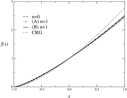
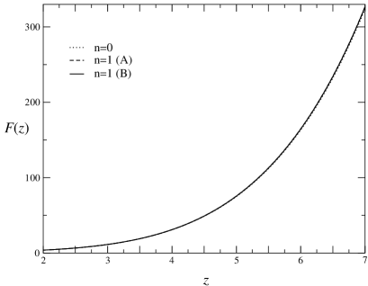
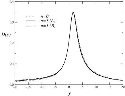
Figure 8: The scaling functions $f(x)$, $F(z)$, and $D(y)$ for the Heisenberg universality class. All results have been obtained in Ref. [234], except those labelled by CRG (Ref. [133]).

5.2.2 Universal amplitude ratios

In Table 27 we report the estimates of several universal amplitude ratios. The results denoted by IHT–PR were obtained in Ref. [234] using approximate parametric representations of the equation of state. The FT estimates of $U_{0}$ were obtained from the analysis of the fixed-dimension expansion in the minimal-renormalization scheme without $\epsilon$ expansion [686, 662] and from the standard $\epsilon$ expansion to $O(\epsilon^{2})$ [137]. The CRG estimate of $U_{0}$ and $R_{\alpha}$ were obtained in Ref. [234] using the expression for $f(x)$ reported in Refs. [133, 134]; they significantly differ from the estimates obtained using other methods. See, e.g., Ref. [932] for a more complete review of theoretical and experimental estimates.

Table 27: Estimates of universal amplitude ratios for the Heisenberg universality class. The numbers marked by an asterisk have been obtained in Ref. [234] using the results reported in the quoted references.

	IHT–PR [234]	$d$=3 exp	$\epsilon$ exp	CRG	HT	experiments
$U_{0}$	1.56(4)	1.51(4) [686]	1.521(22) [137]	∗1.823 [133, 134]		1.50(5) [614]
		1.544 [662]				1.27(9) [762]
						1.4(4) [940]
$R_{\alpha}$	4.3(3)	∗4.4(4) [686]	4.56(9) [137]	∗3.41 [133, 134]
		∗4.46 [662]
$R_{\chi}$	1.31(7)		1.33 [3]	1.11 [133, 134]
$R_{C}$	0.185(10)	0.189(9) [1032]	0.17 [25]
		0.194 [662]
$R_{4}$	7.8(3)
$R_{\xi}^{+}$	0.424(3)	0.4347(20) [71]	0.42 [136]		0.431(5) [215]
		0.4319(17) [138]			0.433(5) [215]
$P_{m}$	1.18(2)
$R_{p}$	2.020(6)

5.2.3 Comparison with the experiments

In spite of the large number of experiments, at present there is no accurate quantitative study of the equation of state in the critical regime. We shall discuss here three different representations that are widely used in experimental work.

A first possibility [674] consists in studying the behavior of $h/m\equiv H|t|^{-\gamma}/M$ versus $m^{2}\equiv M^{2}|t|^{-2\beta}$. Such a function can be easily obtained from approximations of $f(x)$, since $m^{2}=B^{2}|x|^{-2\beta}$ and

$${h\over m}=k|x|^{-\gamma}f(x)$$ (5.2)

where $k=\left(B_{c}\right)^{-\delta}B^{\gamma/\beta}={R_{\chi}/C^{+}}$. A plot of $m^{2}/B^{2}$ versus $C^{+}h/m$ is reported in Fig. 9. It agrees qualitatively with the analogous experimental ones reported, e.g., in Refs. [614, 69, 398].

Often, for small $h/m$ one approximates the equation of state by writing

$${h\over m}=a_{\pm}+b_{\pm}m^{2},$$ (5.3)

where $a_{\pm}$ and $b_{\pm}$ are numerical coefficients depending on the phase. Such an approximation has a limited range of validity. In the HT phase, one obtains for $m^{2}\to 0$ [234]

$${h\over m} = {1\over C^{+}}\left[1+{R_{4}\over 6}{m^{2}\over B^{2}}+\sum_{n=2}^{\infty}{R^{n}_{4}\ r_{2n+2}\over(2n+1)!}\left({m^{2}\over B^{2}}\right)^{n}\right]$$ (5.4)

$$\approx {1\over C^{+}}\Bigl{[}1+1.30(5)\ {m^{2}\over B^{2}}+0.94(8)\ \left({m^{2}\over B^{2}}\right)^{2}+0.06(2)\ \left({m^{2}\over B^{2}}\right)^{3}+\cdots\Bigr{]}.$$

From Eq. (5.4), one sees that the approximation (5.3) is valid only for very small $m^{2}$, i.e. at the 1% level only for $m^{2}\lesssim 0.01B^{2}$. The quadratic approximation—i.e. the approximation with an additional $(m^{2})^{2}$ term—has a much wider range of validity because of the smallness of the coefficient of $m^{6}$.

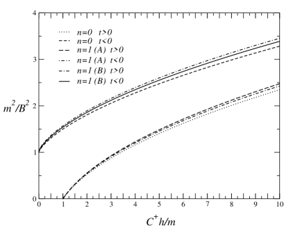
Figure 9: Plot of $m^{2}/B^{2}$ versus $C^{+}h/m$. From Ref. [234].

In the low-temperature phase, Eq. (5.3) is theoretically incorrect, since it does not take into account the presence of Goldstone modes. Indeed, for $m^{2}/B^{2}\to 1$, we have

$${h\over m}\approx{kc_{f}\over 4\beta^{2}}\left(1-{m^{2}\over B^{2}}\right)^{2},$$ (5.5)

where $c_{f}$ is defined in Eq. (1.99). Eq. (5.5) is inconsistent with the approximation (5.3) near the coexistence curve.

Finally, note that for $m^{2}$ large we have

$${h\over m}\approx k\left({m\over B}\right)^{\delta-1}.$$ (5.6)

A second form that is widely used to analyze the experimental data is the Arrott-Noakes [62] scaling equation

$$\left({H\over M}\right)^{1/\gamma}=at+bM^{1/\beta},$$ (5.7)

where $a$ and $b$ are numerical constants. This approximation is good in a neighborhood of the critical isotherm $t=0$. Since

$$\left({H\over M}\right)^{1/\gamma}k^{-1/\gamma}=\left({M\over B}\right)^{1/\beta}f(x)^{1/\gamma},$$ (5.8)

one obtains [234]

$$\left({H\over M}\right)^{1/\gamma}k^{-1/\gamma}=\left({M\over B}\right)^{1/\beta}+0.96(4)\ t-0.04(2)\,t^{2}\left({M\over B}\right)^{-1/\beta}-0.02(2)\,t^{3}\left({M\over B}\right)^{-2/\beta}\cdots$$ (5.9)

Thus, at a 1% level of precision the Arrott-Noakes formula is valid approximately for $t(MB^{-1})^{-1/\beta}\lesssim 25$ which is quite a large interval.

Finally, Ref. [1145] reports an experimental study of the behavior of Tl₂Mn₂O₇ along the crossover line, and determines the scaling function $D(y)$, although with different normalizations. The comparison of their results with the theoretical curve $D(y)$ obtained in Ref. [234], see Sec. 5.2, shows a very nice quantitative agreement.

6 Critical behavior of $N$-vector models with $N\geq 4$

Among the three-dimensional $N$-vector models with $N\geq 4$, the physically most relevant ones are those with $N=4$ and $N=5$. The $N=4$ case is relevant for high-energy physics because it describes the finite-temperature transition in the theory of strong interactions, i.e. quantum chromodynamics (QCD), with two light degenerate flavored quarks. The case $N=5$ might be relevant for superconductivity: indeed, an SO(5) theory has been proposed to explain the critical properties of high-$T_{c}$ superconductors [1144]. In this section we mainly review these two models.

For larger values of $N$, estimates of the critical exponents can be found in Refs. [213, 56]. They are obtained by analyzing 21st-order expansions for the $N$-vector model, and the FT six-loop series at fixed dimension $d=3$.

In the large-$N$ limit one can obtain analytic results based on a $1/N$ expansion. These results are very useful to obtain a qualitative understanding of the critical behavior, but, from a quantitative point of view, they become predictive only for rather large values of $N$, $N\mathrel{\hbox to0.0pt{\lower 3.0pt\hbox{$\mathchar 536\relax$}\hss}\raise 2.0pt\hbox{$\mathchar 318\relax$}}10$ say. We do not further discuss this approach, but we signal the recent review [1154], where many results and references can be found.

We mention that the critical equation of state for the $N$-vector model has been computed to $O(\epsilon^{2})$ in the framework of the $\epsilon$ expansion [182], and to $O(1/N)$ in the framework of the $1/N$ expansion [181].

6.1 The O(4) universality class

The three-dimensional O(4) model is relevant for QCD with two light-quark flavors at finite temperature. This theory shows a finite-temperature transition, in which the quark condensate $\langle\bar{\psi}\psi\rangle$ is the order parameter and the quark mass plays the role of external field. Using symmetry arguments, it has been argued that, if the finite-temperature transition is continuous, it should belong to the same universality class of the three-dimensional O(4) model [914, 1120, 938]. Finite-temperature simulations of lattice QCD [574, 29] support the existence of a continuous phase transition.

In Table 28 we report the theoretical results for the critical exponents of the O(4) symmetric model. They have been obtained by FSS MC simulations for the $N$-vector model [606, 93] and for an improved $\phi^{4}$ theory [515], from the analysis of 21st-order HT expansions [213], using perturbative FT methods [56, 481] and the nonperturbative CRG approach [805, 458]. Numerical studies of the critical equation of state can be found in Refs. [1066, 373].

Table 28: Estimates of the critical exponents for the O(4)-vector model. We indicate with an asterisk (^∗) the estimates that have been obtained using the scaling relations $\gamma=(2-\eta)\nu$, $2-\alpha=3\nu$.

Ref.	info	$\gamma$	$\nu$	$\eta$	$\omega$
[515] 2001	MC FSS $\phi^{4}$	1.471(4)∗	0.749(2)	0.0365(10)	0.765
[93] 1996	MC FSS	1.476(2)∗	0.7525(10)	0.0384(12)
[606] 1995	MC FSS	1.477(18)∗	0.748(9)	0.0254(38)
[213] 1997	HT sc	1.491(4)	0.759(3)	0.035(9)∗
[213] 1997	HT bcc	1.484(4)	0.756(3)	0.037(9)∗
[481] 1998	FT $d=3$ exp	1.456(10)	0.741(6)	0.0350(45)	0.774(20)
[56] 1995	FT $d=3$ exp	1.449	0.738	0.036
[481] 1998	FT $\epsilon$ exp	1.448(15)	0.737(8)	0.036(4)	0.795(30)
[458] 2001	CRG (1st DE)	1.443	0.739	0.047
[805] 1998	CRG (1st DE)	1.614	0.816	0.022

6.2 The O(5) universality class and the SO(5) theory of high-$T_{c}$ superconductivity

The O(5) universality class has not been much studied and, at present, there are only a few estimates of the critical parameters. The critical exponents have been determined using FT methods [56], obtaining $\gamma=1.506$, $\nu=0.766$, and $\eta=0.034$, and by MC simulations [555], finding $\nu=0.728(18)$. Concerning the spin-2 and spin-4 perturbations, see Sec. 1.5.8, we report the following results: $\phi_{2}=1.40(4)$ [227] and $\phi_{4}=0.145(7)$ [230] obtained using FT methods, and $\phi_{2}=1.387(30)$ [555] from MC simulations.

It has been argued that the O(5) universality class is relevant for the description of high-$T_{c}$ superconductivity. In the SO(5) theory [1144], one considers a model with symmetry O(3)$\oplus$U(1) = O(3)$\oplus$O(2) with two order parameters: one is related to the antiferromagnetic order, the other one is associated with $d$-wave superconductivity. Neglecting the fluctuations of the electromagnetic field [498], the most general Hamiltonian with symmetry O(3)$\oplus$O(2) describing the interactions of the two order parameters is

$${\cal H}_{\rm eff}=\int d^{3}x\Bigl{[}{\textstyle\frac{1}{2}}(\partial_{\mu}\phi_{1})^{2}+{\textstyle\frac{1}{2}}(\partial_{\mu}\phi_{2})^{2}+{\textstyle\frac{1}{2}}r_{1}\phi_{1}^{2}+{\textstyle\frac{1}{2}}r_{2}\phi_{2}^{2}+u_{1}(\phi_{1}^{2})^{2}+u_{2}(\phi_{2}^{2})^{2}+w\phi_{1}^{2}\phi_{2}^{2}\Bigr{]},$$ (6.1)

where $\phi_{1}$ is the three-component antiferromagnetic order parameter and $\phi_{2}$ is the two-component superconductivity order parameter. Such Hamiltonian has been extensively studied in the literature, see, e.g. Ref. [669], since it describes a variety of multicritical phenomena. See also Sec. 11.7.

The main issue is whether the SO(5) symmetry can be realized at a bicritical point where two critical lines, with symmetry O(3) and O(2) respectively, meet. In RG terms, this can generally occur if the O(5) fixed point has only two relevant O(3)$\oplus$ O(2)-symmetric perturbations. On the other hand, as shown in Ref. [230], (at least) three relevant perturbations exist: beside the usual O(5)-symmetric interaction associated with the temperature, there are two perturbations with O(5)-spin 2 and 4 respectively (explicit formulae are given in Sec. 11.3 and in Ref. [230]) that are relevant, since $\phi_{2}>0$ and $\phi_{4}>0$ (see the estimates reported above). The stable fixed point is expected to be the tetracritical decoupled fixed point. Indeed, using nonperturbative arguments one can show [18, 19] that the RG dimension $y_{w}$ associated with the perturbation $w\phi_{1}^{2}\phi_{2}^{2}$ of the decoupled fixed point is negative, i.e. the perturbation is irrelevant. This follows from

$$y_{w}={1\over 2}\left({\alpha_{XY}\over\nu_{XY}}+{\alpha_{O(3)}\over\nu_{O(3)}}\right)<0.$$ (6.2)

As a consequence, the SO(5) fixed point can only be reached by tuning an additional parameter.

These conclusions are in apparent contrast with the MC results of Ref. [555], that seem to favor the picture based on a stable bicritical O(5) fixed point. On the other hand, as suggested by Aharony [18], the MC data of Ref. [555] may just show a slow crossover towards either the stable tetracritical decoupled point or a weak first-order transition. This hypothesis is somehow supported by the small value of the crossover exponent $\phi_{4}$ at the O(5) fixed point, i.e. $\phi_{4}=0.145(7)$.

7 The two-dimensional $XY$ universality class

7.1 The Kosterlitz-Thouless critical behavior

The two-dimensional $XY$ universality class is characterized by the Kosterlitz-Thouless (KT) critical behavior [670, 668] (see, e.g., Refs. [570, 1152] for reviews on this issue). According to the KT scenario, the free energy has an essential singularity at $T_{c}$ and the correlation length diverges as

$$\xi\sim\exp\left({b/t^{\sigma}}\right)$$ (7.1)

for $t\equiv T/T_{c}-1\to 0^{+}$. The value of the exponent is $\sigma=1/2$ and $b$ is a nonuniversal positive constant. At the critical temperature, the asymptotic behavior for $r\rightarrow\infty$ of the two-point correlation function should be

$$G(r)_{\rm crit}\sim{(\ln r)^{2\theta}\over r^{\eta}}\,\left[1+O\left({\ln\ln r\over\ln r}\right)\right],$$ (7.2)

with $\eta=1/4$ and $\theta=1/16$. Near criticality, i.e., for $0<t\ll 1$, the behavior of the magnetic susceptibility can be derived from Eq. (7.2):

$$\chi\sim\int_{0}^{\xi}dr\,G(r)_{\rm crit}\sim\xi^{2-\eta}\left(\ln\xi\right)^{2\theta}\left[1+O\left({\ln\ln\xi\over\ln\xi}\right)\right]\sim\xi^{2-\eta}t^{-2\sigma\theta}\left[1+O\left(t^{\sigma}\ln t\right)\right].$$ (7.3)

In addition, the two-dimensional $XY$ model is characterized by a line of critical points, starting from $T_{c}$ and extending to $T=0$, with $\eta\sim T$ for $T\rightarrow 0$. At criticality the two-dimensional $XY$ model corresponds to a conformal field theory with $c=1$, see, e.g., Ref. [570].

Transitions of KT type occur in a number of effectively two-dimensional systems with O(2) symmetry, such as thin films of superfluid helium and of easy-plane magnetic materials. In particular, planar ferromagnets are realized by layered compounds such as K₂CuF₄ [544] and Rb₂CrCl₄ [559, 36] that effectively behave as two-dimensional systems. The crossover from two-dimensional to three-dimensional behavior has been observed in CoCl₂ intercalated in graphite [1119], in Gd₂CuO₄ [789], and in YBa₂Cu₃O_6+x [797]. We also mention the experimental results of Ref. [131] for iron films epitaxially grown on GaAs(001).

The KT critical scenario describes roughening transitions, i.e. phase transitions from a smooth to a rough surface, which are, for example, observed in the equilibrium structure of crystal interfaces. For a general introduction to roughening, see, e.g., Refs. [4, 1074, 440, 570]. At a roughening transition, the large-scale interface behavior changes from being smooth at low temperature to being rough at high temperature. This qualitative picture can be made quantitative, for example by looking at the dependence of the interfacial width on the size $L$ of the interface: in the smooth phase the interfacial width remains finite when $L\to\infty$, while it diverges logarithmically in the rough phase.

7.2 The roughening transition and solid-on-solid models

The interfacial thermodynamic behavior can be modeled by solid-on-solid (SOS) models defined on two-dimensional lattices. The partition function of a SOS model is

$$Z=\sum_{\{h\}}\exp\Bigl{[}-\sum_{\langle xy\rangle}V(h_{x}-h_{y})\Bigr{]},$$ (7.4)

where the Hamiltonian is a sum over nearest-neighbor pairs. The variables $h_{x}$ can be interpreted as heights with respect to a certain base. The summation is over equivalence classes of height configurations $\{h\}$, defined by identifying two configurations that differ only by a global vertical shift. Several realizations of the SOS model have been proposed, see, e.g., Refs. [4, 1074, 518]. We mention:

• The absolute-value SOS model (ASOS). It can be considered as the SOS approximation of a lattice plane interface of an Ising model on a simple cubic lattice, and it is defined by the function

  $$V_{\rm ASOS}=k|h_{x}-h_{y}|,$$ (7.5)

  where $h_{x}$ takes integer values. For finite positive $k$ the Hamiltonian suppresses configurations with large differences between nearest-neighbor sites. If $k$ is below a certain critical value, the surface becomes rough, and the surface thickness diverges when the size of the system goes to infinite.

• The body-centered SOS model (BCSOS). It represents a SOS approximation of an interface in an Ising model on a bcc lattice [1073].

• The discrete Gaussian (DG) model defined by

  $$V_{\rm ASOS}=k(h_{x}-h_{y})^{2},$$ (7.6)

  where $h_{x}$ takes integer values. It is dual to the Villain formulation of the $XY$ model [979].

• The dual of the standard $XY$ model,

  $$H_{XY}=-\beta\sum_{\langle xy\rangle}\vec{s}_{x}\cdot\vec{s}_{y},$$ (7.7)

  can be considered as a SOS model with partition function

  $$Z=\sum_{\{h\}}\prod_{\langle xy\rangle}I_{|h_{x}-h_{y}|}(\beta),$$ (7.8)

  where $h_{x}$ are integer variables and $I_{n}$ are modified Bessel functions.

The BCSOS model is the only one that has been proved to undergo a KT transition [1073]. It can be transformed into the $F$ model [1073], which is a special six-vertex model that can be solved exactly using transfer-matrix methods [703, 704, 111]. The transitions in the other models, including the standard $XY$ model, are conjectured to be of the KT type as well, and numerical evidences support this fact.

A much studied prototype of roughening is the Ising interface transition, which occurs in the LT phase of the three-dimensional Ising model, i.e. for $T_{r}<T_{c}$ where $T_{c}$ is the bulk critical temperature [1103, 517]. The SOS approximation amounts to neglecting overhangs of the Ising interface and bubbles in the two phases separated by the interface. Lattice studies of the interfacial properties use the fact that an interface of size $L$ can be realized on a $L^{2}\times T$ lattice by imposing antiperiodic boundary conditions along the third direction.

Roughening transitions also occur in the lattice formulation of four-dimensional nonabelian gauge theories [1123], which, in the critical limit $T\rightarrow 0$, provide a nonperturbative definition of QCD, the theory of strong interactions. See, e.g., Refs. [308, 798] for an introduction to lattice gauge theories. An important issue concerning nonabelian gauge theories is related to confinement. In the absence of quarks, the question of confinement is related to the behavior of the Wilson loop in the limit of large area. Confinement requires a nonzero string tension $\sigma$. In the HT region $\sigma$ is not zero. For $T\to\infty$ it behaves as $\sigma\sim\ln T$, with $T^{-n}$ corrections that can be systematically computed. Theoretical arguments show that, independently of the gauge group, the string tension is affected by a weak singularity associated with the roughening transition [881, 522, 572, 740, 741, 354, 820] (see also Ref. [570]). However, the roughening transition does not imply deconfinement, and the string tension should not vanish in the weak-coupling region, and therefore in the continuum limit. The change is essentially related to the fact that at strong coupling the contributions to the string tension come from smooth surfaces, while in the weak coupling region the relevant surfaces become rough.

7.3 Numerical studies

Numerical studies of the $XY$ model based on MC simulation techniques, HT expansions, and CRG methods support the KT behavior [148, 89, 582, 516, 862, 992, 626, 636, 581, 518, 458].

In MC simulations, FSS investigations at criticality must be very precise in order to pinpoint the logarithm in the two-point Green’s function, cf. Eq. (7.2). On the other hand, if this logarithmic correction is neglected, i.e. one sets $\theta=0$, a precise check of the prediction $\eta=1/4$ at $\beta_{c}$ may be quite hard. The relevance of such logarithmic corrections and some of the consequences of neglecting them have been examined in Refs. [626, 581].

HT expansion calculations [209, 210, 237] support the KT mechanism as well. In Ref. [237] the two-point correlation function was calculated on the square, triangular, and honeycomb lattices respectively up to 21st, 15th, and 30th order. The results from all considered lattices were consistent with universality and the KT exponential approach (7.1). The prediction $\sigma=1/2$ has been confirmed with an uncertainty of few per cent. The prediction $\eta=1/4$ has been also substantially verified.

On the other hand, the value of $\theta$ predicted by the KT theory, i.e. $\theta=1/16$, has not yet got a direct robust numerical confirmation. Some discrepancies have been noted in the results of MC simulations [626, 581] and HT expansions [237]. But one should be cautious in considering these results as a real inconsistency, since it is difficult to exclude a substantial underestimate of the error.

The most accurate verification of the KT critical pattern was achieved in Refs. [516, 517], by numerically matching the RG trajectory of the dual of the $XY$ model with that of the BCSOS model, which has been proven to exhibit a KT transition. The advantage of this strategy is that such a matching occurs much earlier than the onset of the asymptotic regime, where numerical simulations can provide quite accurate results. Indeed, the authors argued that their method is subject to corrections due to irrelevant operators, which are of order $L^{-\omega}$ with $\omega=2$, while standard MC results are affected by logarithmic corrections. In Refs. [516, 517] the same method was applied to the ASOS model, the DG model, and the interface in a simple-cubic Ising model, in order to demonstrate that they all belong to the same universality class, and therefore undergo a KT transition.

Finally, we mention the results available for the critical limit $g_{4}^{+}$ of zero-momentum four-point coupling $g_{4}$, defined in Eq. (2.3), and the small-magnetization expansion of the Helmholtz free energy. In Table  29 we review the estimates of $g_{4}^{+}$ obtained by various approaches: high-temperature series (HT), Monte Carlo simulations (MC), field-theoretical methods (FT), and the form-factor approach (FF). The first few coefficients $r_{2j}$ of the small-magnetization expansion of the scaling equation of state, cf. Eq. (1.80), were estimated in Ref. [907] by a constrained analysis of their $O(\epsilon^{3})$ series, obtaining $r_{6}=3.53(4)$ and $r_{8}\approx 23$.

Results concerning the small-momentum behavior of the two-point function in the HT phase can be found in Ref. [237].

Table 29: Estimates of $g_{4}^{+}$ for the two-dimensional $XY$ universality class.

HT	MC	FT $d=2$ exp	FT $\epsilon$ exp	FF
13.65(8) [904]	13.71(18) [101]	13.57(23) [870]	13.7(2) [907]	13.65(6) [102]
13.72(16) [211]	13.3(3) [637]

8 Two-dimensional $N$-vector models with $N\geq 3$

Two-dimensional $N$-vector models with $N\geq 3$ are somewhat special since in this case there is no phase transition at finite values of $T$. The correlation length is always finite and a critical behavior is observed only when $T\to 0$.

For $T\to 0$ the behavior of long-distance quantities is predicted by the perturbative RG applied to the $N$-vector model. One finds that these systems are asymptotically free with a nonperturbatively generated mass gap [922, 183, 185, 106]. Such a property is also present in QCD, i.e. the theory of strong interactions, and thus these two-dimensional theories are often used as toy models in order to understand nonperturbative properties and to test numerical methods that are of interest for the more complex theory of QCD (see, e.g., Ref. [923]).

The two-dimensional $N$-vector model is also important in condensed-matter physics. For $N=3$ it describes the behavior for $T\to 0$ of the two-dimensional spin-$S$ Heisenberg quantum antiferromagnet [281]. Indeed, at finite temperature $T$ this quantum spin system is described by a (2+1)-dimensional $O(3)$ classical theory in which the Euclidean time direction has a finite extent $1/T$. In the critical limit the relation $1/T\ll\xi$ is satisfied, therefore the system becomes effectively two-dimensional, and thus its critical behavior is described by the two-dimensional three-vector model.

Moreover, the non-linear FT formulation of the two-dimensional $N$-vector model with $N\geq 3$ is the starting point for the $\varepsilon\equiv d-2$ expansion (see, e.g., Ref. [1152] and references therein), which provides information of the critical properties of $N$-vector models for $d\mathrel{\hbox to0.0pt{\lower 3.0pt\hbox{$\mathchar 536\relax$}\hss}\raise 2.0pt\hbox{$\mathchar 318\relax$}}2$. The $\varepsilon$ expansion of the critical exponents is known to $O(\varepsilon^{4})$ [542, 541, 135]. Contrary to what happens for the $\epsilon=4-d$ expansion, $\varepsilon$-series have limited application and do not provide quantitative predictions for physical three-dimensional transitions, essentially because they are not Borel summable [542] and it is not known how to resum them. An attempt based on a variational approach was presented in Ref. [656].

Beside being asymptotically free, the two-dimensional $N$-vector model with $N\geq 3$ has another remarkable property. The corresponding quantum field theory is integrable, in the sense that, assuming asymptotic freedom, one can establish the existence of nonlocal conserved charges and the absence of particle production [739, 201, 202]. This implies the existence of a factorized $S$-matrix [1141] and allows the application of powerful techniques, such as the thermodynamic Bethe Ansatz and the form-factor bootstrap approach (the latter has been applied only to the $N=3$ case). These approaches have led to exact predictions for several nonperturbative quantities [524, 525, 607, 744, 99, 100, 101].

8.1 The critical behavior

The critical behavior for $T\to 0$ can be computed in perturbation theory for a particular class of $O(N)$ models that, in this context, are usually called $\sigma$-models. On the lattice one may consider Hamiltonians

$${\cal H}=-{1\over T}\sum_{ij}K(i-j)\vec{s}_{i}\cdot\vec{s}_{j},$$ (8.1)

where $K(x)$ is a short-range coupling and $|\vec{s}_{i}|=1$. If only nearest-neghbor spins are coupled, we reobtain the $N$-vector model (1.4). It is also possible to add couplings that involve more than two spins without changing the universality class. The only important requirement is that the ground state of the system is ferromagnetically ordered.

For this class of systems we can use spin-wave perturbation theory and the RG to obtain the behavior for $T\to 0$. See, e.g., Ref. [1152] for a general reference. For the true correlation length $\xi_{\rm gap}$ and the susceptibility $\chi$ one has

$$\xi_{\rm gap}(T) = \xi_{0}\left({\beta_{0}T}\right)^{\beta_{1}/\beta_{0}^{2}}\exp\left({1\over\beta_{0}T}\right)\,\exp\left[\int_{0}^{T}dt\left({1\over\beta(t)}+{1\over\beta_{0}t^{2}}-{\beta_{1}\over\beta_{0}^{2}t}\right)\right],$$ (8.2)

$$\chi(T) = \chi_{0}\left({\beta_{0}T}\right)^{2\beta_{1}/\beta_{0}^{2}+\gamma_{0}/\beta_{0}}\exp\left({2\over\beta_{0}T}\right)\times$$ (8.3)

$$\exp\left[\int_{0}^{T}dt\,\left({2\over\beta(t)}+\,{2\over\beta_{0}t^{2}}-\,{2\beta_{1}\over\beta_{0}^{2}t}-{\gamma(t)\over\beta(t)}-\,{\gamma_{0}\over\beta_{0}t}\right)\right],$$

where $\beta(T)$ is the $\beta$-function, defined by $\beta(T)=-adT/da$ with $a$ being the lattice spacing, and $\gamma(T)$ is the anomalous dimension of the field. These functions describe how the temperature and the fundamental field should vary with the lattice spacing $a$ to keep the renormalized Green’s functions fixed. They have a perturbative expansion of the form

$$\beta(T)=-T^{2}\sum_{n=0}\beta_{n}T^{n},\qquad\gamma(T)=T\sum_{n=0}\gamma_{n}T^{n},$$ (8.4)

and are model-dependent. However, two particular combinations of the perturbative coefficients are universal, $\beta_{1}/\beta_{0}^{2}$ and $\gamma_{0}/\beta_{0}$, that appear as universal exponents in the critical behavior of $\xi$ and $\chi$. Explicitly:

$${\beta_{1}\over\beta_{0}^{2}}={1\over N-2},\qquad{\gamma_{1}\over\beta_{0}}={N-1\over N-2}.$$ (8.5)

The perturbative expansions of $\beta(T)$ and $\gamma(T)$ have been determined for several different models: to four-loop order for the continuum theory in the minimal subtraction scheme [135] and for the standard $N$-vector model [259, 33], and to three-loop order for several other theories [378, 258, 35].

The nonperturbative constants $\xi_{0}$ and $\chi_{0}$ are also nonuniversal. The ratio of $\xi_{0}$ (and also of $\chi_{0}$) in two different models can be computed in one-loop perturbation theory. For the $N$-vector model with nearest-neighbour interactions, $\xi_{0}$ was computed exactly by means of the thermodynamic Bethe Ansatz [524, 525]:

$$\xi_{0}=\left({e\over 8}\right)^{1/(N-2)}\Gamma\left({N-1\over N-2}\right)2^{-5/2}\exp\left(-{\pi\over 2(N-2)}\right).$$ (8.6)

For $N=3$, there also exists a precise estimate of $\chi_{0}$ obtained by combining the form-factor approach and HT expansions [238], $\chi_{0}=0.01452(5)$. Of course, one can consider other thermodynamic functions. In order to obtain the corresponding low-$T$ behavior, the anomalous dimensions are needed. For some composite operators, perturbative expressions can be found in Refs. [184, 258, 257].

The predictions (8.2) and (8.3) also apply to more general models in which the fields do not satisfy the condition $\vec{\phi}\cdot\vec{\phi}=1$, for instance to the $\phi^{4}$ theory (1.7). In this case, however, the functions $\beta(T)$ and $\gamma(T)$ cannot be determined analytically.

The perturbative predictions have been checked in several different ways. The results for $\chi$ and $\xi$ have been checked in the large-$N$ limit, including the nonperturbative constant (8.6), to order $1/N$ [154]. Several simulations checked the predictions for $N=3$, 4, and 8 [1132, 362, 244, 253, 251, 785, 32, 34] for the standard $N$-vector model and some other lattice versions in the same universality class. For $N=3$ there are significant discrepancies (of order 15-20%) between MC results and 4-loop perturbative results at correlation lengths of order 100. This discrepancy decreases significantly at $\xi\approx 10^{5}$ where it is approximately 4%. For larger values of $N$ the agreement is better and for $\xi\approx 100$ 4-loop perturbation theory differs from MC results by 4% ($N=4$) and 1% ($N=8$). The agreement improves if one considers the so-called “improved” perturbation theory [882, 884] in terms of effective temperature variables, which take somehow into account a large part of the perturbative contributions (see the discussions of Refs. [258, 958]). The corresponding perturbative results are in better agreement with the numerical ones [251, 32, 34].

It is interesting to mention that, at variance with the three-dimensional case, the $1/N$ expansion is quite predictive even for $N=3$ [433, 236].

As already mentioned, the above results can be extended to the antiferromagnetic quantum Heisenberg model on a square lattice, with Hamiltonian

$${\cal H}={1\over T}\sum_{<xy>}\vec{s}_{x}\cdot\vec{s}_{y},$$ (8.7)

where $\vec{s}_{x}$ is a spin operator satisfying the commutation relations $[s_{x,i},s_{y,j}]=\delta_{xy}\epsilon_{ijk}s_{x,k}$ and the condition $s_{x}^{2}=S(S+1)$. For $T\to 0$, the correlation length can be computed obtaining [281, 526, 523]

$$\xi_{\rm gap}={e\over 8}{c\over 2\pi\rho_{s}}\exp\left({2\pi\rho_{s}\over T}\right)\left(1-{T\over 4\pi\rho_{s}}+O(T^{2})\right)f(\gamma),$$ (8.8)

where $\rho_{s}$ is the spin stiffness, $c$ the spin-wave velocity, $\gamma=2S/T$, and $f(\gamma)$ a function computed numerically in Ref. [523] and which has the limit values: $f(\infty)=1$, $f(\gamma)=e^{-\pi/2}/(8\gamma)$ for $\gamma\to 0$. Of course, for $S\to\infty$ we reobtain the low-$T$ behavior of the classical model. These results have been compared with the experimental and the numerical results obtained for the antiferromagnet. Similarly to the classical model, good agreement is observed only for very large values of the correlation length [640, 642, 114, 115].

8.2 Amplitude ratios and two-point function

The RG predictions (8.2) and (8.3) are quite difficult to test because the neglected corrections are powers of $T$, thus corresponding to powers of $\log\xi$. As a consequence, numerical determinations of the nonperturbative constants $\xi_{0}$ and $\chi_{0}$ are extremely difficult. On the other hand, in the case of RG invariant quantities scaling corrections are negative integer powers of $\xi$, apart from logarithms. Indeed, models with $N\geq 3$ are essentially Gaussian and thus the operators have canonical dimensions. For a generic RG invariant quantity we expect:

$$R(T)=R^{*}+b{X^{p}\over\xi^{2}}\left(1+{a_{1}\over X}+{a_{2}\log X\over X^{2}}+{a_{3}\over X^{2}}+\ldots\right)+O\left(\xi^{-4}\right),$$ (8.9)

where $X\equiv\log\xi$. Apart from logarithmic corrections, the exponent associated with the leading scaling corrections is given by $\omega=2$. Such a behavior is verified explicitly in large-$N$ calculations, see, e.g., Ref. [223]. This means that accurate estimates of the universal constants $R^{*}$ can be obtained by determining $R(T)$ at values of $T$ corresponding to relatively small $\xi$.

The approach to scaling can be somehow improved by considering models in which some scaling corrections vanish. In the context of asymptotically free theories, one can determine analytically, using perturbation theory, the Hamiltonian parameters that provide the cancellation of the leading logarithms associated with each power correction [1040, 1041]. However, in practice the obtainable improvement using this approach is rather modest: the scaling corrections change only by powers of $\log\xi$. Several improved models of this type have been considered in Refs. [1041, 527, 959, 256]. On the other hand, a complete removal of the $O(\xi^{-2})$ scaling corrections would require the tuning of an infinite numbers of parameters.

In Table 30 we review the estimates of the four-point coupling constant $g_{4}^{+}$ for $N=3$ obtained by various approaches, such as the form-factor approach (FF), Monte Carlo simulations (MC), high-temperature series (HT), and field-theoretical methods (FT). The agreement is globally good. We only note that the HT results of Refs. [904, 236] are slightly smaller than the precise FF and MC estimates. The HT estimates were taken at a value of the temperature corresponding to a correlation length $\xi\approx 10$, where the HT analysis was reliable. The difference with the other results should be essentially due to an underestimate of the scaling corrections. Concerning the coefficients $r_{2n}$ that parametrize the equation of state for $M\to 0$, we mention the estimates $r_{6}=3.33(2)$ and $r_{8}\approx 19$ for $N=3$, obtained by a constrained analysis of their $O(\epsilon^{3})$ series [907]. For $N\geq 4$, estimates of $g_{4}^{+}$ and of the first few $r_{2n}$ can be found in Refs. [236, 211, 904, 907].

Table 30: Estimates of $g_{4}^{+}$ for the two-dimensional O(3) universality class.

FF	MC	HT	FT $d=2$ exp	FT $\epsilon$ exp
12.19(3) [100]	12.21(4) [100, 101]	11.82(6) [904]	12.00(14) [870]	12.0(2) [907]
	11.9(2) [637]	11.9(2) [236]	11.99(11) [377]

Finally, let us discuss the two-point function. Similarly to three-dimensional models, the scaling function $g^{+}(y)$ defined in Eq. (1.126) is well approximated by the Ornstein-Zernike behavior $g^{+}(y)\approx 1+y$ up to $y\approx 1$. Indeed, the constants $c_{n}^{+}$ defined in Eq. (1.128) are very small . For instance, for $N=3$ the HT analysis of Ref. [238] obtained $c_{2}^{+}=-0.0012(2)$, $|c_{3}|\mathrel{\hbox to0.0pt{\lower 3.0pt\hbox{$\mathchar 536\relax$}\hss}\raise 2.0pt\hbox{$\mathchar 316\relax$}}10^{-4}$, $S_{M}^{+}=0.9987(2)$ and $S_{Z}^{+}=1.0025(4)$, cf. Eqs. (1.128) and (1.131). The most precise estimate of $S_{M}^{+}$ was obtained by means of the form-factor approach, obtaining $S_{M}^{+}=0.998350(2)$ [100]. For $N=3$, $S_{M}^{+}$ has also been determined by means of MC simulations, obtaining $S_{M}^{+}=0.9985(12)$ [787] and $S_{M}^{+}=0.996(2)$ [32]. The overall agreement is good.

For large values of $q^{2}$, there are logarithmic deviations from the Ornstein-Zernike behavior. For $y\to\infty$ we have

$$g^{+}(y)\sim y(\ln y)^{-1/(N-2)}.$$ (8.10)

In $x$-space this implies, for $x\to 0$:

$$G(x)\sim(\ln 1/x)^{N-1\over N-2}.$$ (8.11)

Finally, we report the result of Ref. [99] for the asymptotic behavior of $Z_{\rm gap}$, see Eq. (1.130). For $T\to 0$

$$Z_{\rm gap}(T)=C(N)(\beta_{0}T)^{{\textstyle\frac{N-1}{N-2}}}\left[1+O(T)\right].$$ (8.12)

The constant $C(N)$ is exactly known for $N=3$: $C(3)=3\pi^{3}$ [99].

9 The limit $N\to 0$, self-avoiding walks, and dilute polymers

In this section we discuss the limit $N\to 0$ of the $N$-vector model. This is not an academic problem as it may appear at first. Indeed, in this limit, the $N$-vector model describes the statistical properties of linear polymers in dilute solutions and in the good-solvent regime, i.e. above the $\Theta$ temperature [325, 334, 432, 442]. Note that FT methods can also be applied to describe the full crossover from the dilute to the semidilute regime, and, in particular, to compute the universal scaling behavior of the osmotic pressure in terms of the concentration [334, 442, 330, 335, 663].

9.1 Walk models

Several walk models can be mapped into scalar theories with an $N$-vector field in the limit $N\to 0$. They belong to the same universality class of polymers in dilute solutions in the good-solvent regime, and thus their study provides quantitative predictions for the statistical behavior of long macromolecules.

We begin by introducing the random walk (RW) and the self-avoiding walk (SAW). Given a regular lattice, an $n$-step lattice RW is a collection of lattice points $\{\omega_{0},\ldots,\omega_{n}\}$ such that, for all $k$, $1\leq k\leq n$, $\omega_{k}$ and $\omega_{k-1}$ are lattice nearest neighbors. A lattice SAW is a nonintersecting lattice RW, i.e. a walk such that $\omega_{i}\not=\omega_{j}$ for all $i\not=j$. Analogously, an $n$-step self-avoiding (rooted) polygon (SAP) is defined as a closed $n$-step RW such that $\omega_{0}=\omega_{n}$ and $\omega_{i}\not=\omega_{j}$ for all $0\leq i\not=j\leq n-1$.

Several quantities are usually introduced for SAW’s and SAP’s. We define:

• The number $c_{n}(x,y)$ of $n$-step SAW’s going from $x$ to $y$ and the number $c_{n}$ of $n$-step SAW’s starting from any given point (by translation invariance it does not depend on the chosen point).

• The number $p_{n}$ of $n$-step SAP’s starting at a given point.

• The squared end-to-end distance of a SAW $\omega$

  $$R^{2}_{e}(\omega)=(\omega_{n}-\omega_{0})^{2},$$ (9.1)

  and its mean-value $R^{2}_{e}(n)$ over all $n$-step SAW’s, i.e.

  $$R^{2}_{e}(n)={1\over c_{n}}\sum_{\{\omega\}}R^{2}_{e}(\omega)={1\over c_{n}}\sum_{x}|x|^{2}c_{n}(0,x).$$ (9.2)

• The radius of gyration of a SAW or SAP $\omega$

  $$R^{2}_{g}(\omega)={1\over 2(n+1)^{2}}\sum_{i,j=0}^{n}(\omega_{i}-\omega_{j})^{2},$$ (9.3)

  and its mean value $R^{2}_{g}(n)$ over all $n$-step SAW’s.

• The end-to-end distribution function of $n$-step SAW’s

  $$P_{n}(x)={c_{n}(0,x)\over c_{n}}.$$ (9.4)

• The form factor of $n$-step SAW’s or SAP’s

  $$H_{n}(q)={1\over(n+1)^{2}}\left\langle\sum_{i,j=0}^{n}\exp[iq\cdot(\omega_{i}-\omega_{j})]\right\rangle,$$ (9.5)

  where the average is over all $n$-step SAW’s.

• The number $b_{n}$ of pairs of $n$-step SAW’s $(\omega_{1},\omega_{2})$ such that $\omega_{1}$ starts at the origin, $\omega_{2}$ starts anywhere, and $\omega_{1}$ and $\omega_{2}$ have at least one point in common.

The quantities that we have defined have a natural interpretation. The end-to-end distance and the radius of gyration define the typical dimension of the walk and correspond to the correlation length in spin systems. The end-to-end distribution function is the walk analogue of the two-point function in spin systems, while the form factor is the quantity that is relevant in scattering experiments. Finally, the number $b_{n}$ is related to the second virial coefficient $B_{n}=b_{n}/c_{n}^{2}$ that appears in the expansion of the osmotic pressure in powers of the concentration, see, e.g., Ref. [334]. It measures the excluded volume between a pair of SAW’s. For $n\to\infty$, these quantities obey general scaling laws:

$$c_{n}\sim\mu^{n}n^{\gamma-1},\qquad p_{n}\sim\mu^{n}n^{\alpha-2},\qquad b_{n}\sim\mu^{2n}n^{d\nu+2\gamma-2},$$

$$R^{2}_{e}(n)\approx a_{e}n^{2\nu},\qquad R^{2}_{g}(n)\approx a_{g}n^{2\nu}.$$ (9.6)

The constants $\gamma$, $\alpha$, and $\nu$ are critical indices. They are universal in the sense that any walk model which includes the basic property of SAW’s, i.e. the local self-repulsion, has the same scaling behavior with exactly the same critical indices. The names of the indices were given by analogy with the $N$-vector model. Indeed, as we shall discuss in the next section, $\gamma$, $\alpha$, and $\nu$ are respectively the exponents of the susceptibility, of the specific heat, and of the correlation length in the corresponding spin system in the limit $N\to 0$. The quantities $\mu$, $a_{e}$, and $a_{g}$ are instead nonuniversal and depend on the specific model one is considering. Some amplitude ratios are however universal, such as

$$A={a_{g}\over a_{e}}=\lim_{n\to\infty}{R^{2}_{g}(n)\over R^{2}_{e}(n)},\qquad\qquad\Psi=\left({d\over 12\pi}\right)^{d/2}\lim_{n\to\infty}{b_{n}\over c_{n}^{2}[R_{g}^{2}(n)]^{d/2}}.$$ (9.7)

The universality of $A$ follows from the existence of a unique length scale at criticality. The universality of the interpenetration ratio $\Psi$ is more subtle, and it is related to a hyperscaling relation among critical indices—such a relation has already been used in writing the scaling of $b_{n}$ in Eq. (9.6).

The SAW is a good model for dilute linear polymers in a good solvent. Indeed, many properties of dilute polymers in the limit of a large number of monomers are universal and depend essentially on the following properties [325, 334, 432, 442]:

• The polymer can be considered as a continuous completely flexible chain above the persistence-length scale.

• The interaction between monomers is strongly repulsive at small distances: Clearly two monomers cannot occupy the same position in space.

• Above the $\Theta$-temperature (good-solvent regime) the effective long-range attractive interaction between monomers can be neglected: The energetic attraction is much smaller than the entropic repulsion.

The SAW satisfies these properties, and therefore it belongs to the same universality class of real polymers. However, this is not the only model that one can consider, and indeed, many others have been introduced in the literature:

• Domb-Joyce model. This is again a lattice walk model, in which one considers RW’s with Hamiltonian

  $$H(\omega)=w\sum_{i,j}\delta_{\omega_{i},\omega_{j}}.$$ (9.8)

  For $w\to\infty$, all intersections are suppressed and one recovers the SAW model. The Domb-Joyce model interpolates between the RW and the SAW model and offers the possibility of constructing an improved lattice walk model, i.e. a model in which the leading correction to scaling has a vanishing amplitude [125]. The improved Domb-Joyce model corresponds to $\omega\equiv 1-e^{-w}\approx 0.397$.

• Off-lattice models. The SAW and the Domb-Joyce models are defined on a lattice. However, it is also possible to consider models of paths in continuous space. For instance, one can consider a model of off-lattice SAW’s defined as a collection of points $\{\omega_{0},\ldots,\omega_{n}\}$, $\omega_{i}\in\mathbb{R}^{d}$, such that $|\omega_{i}-\omega_{j}|\geq 2a$ for all $i\not=j$, where $a$ is the excluded radius. These walks are weighted with Hamiltonian

  $$H(\omega)=\sum_{i=0}^{n-1}V(\omega_{i}-\omega_{i+1}),$$ (9.9)

  where $V(x)$ is an attractive potential. Two common choices are: $V(x)=\delta(|x|-b)$ (stick-and-ball model) and $V(x)={b\over 2}x^{2}$. The stick-and-ball model is improved, i.e. the coefficient of the leading scaling correction vanishes, for $a/b\approx 0.2235$ [726].

• Continuous models. For theoretical considerations it is useful to consider continuous paths, i.e. generic functions $r(s)$ with $0\leq s\leq n$, $n$ being the length of the path, with Hamiltonian [361]

  $$H[r(s)]=-{1\over 4}\int_{0}^{n}ds\left({d{r}(s)\over ds}\right)^{2}-{w\over 2}\int_{0}^{n}ds\,\int_{0}^{n}dt\,\delta[{r}(s)-{r}(t)]\;.$$ (9.10)

9.2 $N$-vector model for $N\to 0$ and self-avoiding walks

In this section we derive the relation between SAW’s and the limit $N\to 0$ of the $N$-vector model [315, 325, 369]. Consider $N$-vector spin variables $\vec{s}$, the lattice Hamiltonian

$$H=-N\sum_{\langle ij\rangle}\vec{s}_{i}\cdot\vec{s}_{j},$$ (9.11)

where the sum is extended over all nearest-neighbor pairs, and the partition function

$$Z=\int\prod_{i}d\Omega(s_{i})e^{-\beta H},$$ (9.12)

where $d\Omega(s_{i})$ is the invariant normalized measure on the sphere. The limit $N\to 0$ follows immediately from a basic result due to de Gennes (see, e.g., Ref. [325]). If

$$I^{\alpha_{1},\ldots,\alpha_{n}}=\lim_{N\to 0}N^{k/2}\int d\Omega(s)s^{\alpha_{1}}\ldots s^{\alpha_{k}},$$ (9.13)

then

$$I^{\alpha_{1},\ldots,\alpha_{n}}=\cases{\delta_{\alpha_{1}\alpha_{2}}&\qquad if $k=2$,\cr 0&\qquad otherwise.}$$ (9.14)

Thus, for $N\to 0$, we can rewrite the partition function as

$$Z=\int\prod_{i}d\Omega(s_{i})\prod_{\langle ij\rangle}(1+N\beta\vec{s}_{i}\cdot\vec{s}_{j})+O(N^{2}).$$ (9.15)

Then, expanding the product over the links and performing the integration, we obtain a sum over a gas of self-avoiding loops. Each closed loop carries a power of $N$, so that

$$Z=1+NV\sum_{n}{p_{n}\over n}\beta^{n}+O(N^{2}),$$ (9.16)

where $V$ is the volume of the lattice, which is assumed to go to infinity. The factor $1/n$ is due to the fact that each loop can be considered as a SAP rooted in $n$ different points. Then, using the asymptotic behavior (9.6), we obtain for $\beta\to 1/\mu$, and $V\to\infty$

$$\lim_{N\to 0}{1\over NV}\log Z=\sum_{n=0}^{\infty}{p_{n}\over n}\beta^{n}\sim(\beta-1/\mu)^{2-\alpha}.$$ (9.17)

We thus see that $\alpha$ is the specific-heat exponent and we may interpret $1/\mu$ as the critical temperature of the model.

Let us now compute the two-point function. Repeating the argument given above, we obtain

$$\lim_{N\to 0}G(x-y)=\lim_{N\to 0}\langle\vec{s}_{x}\cdot\vec{s}_{y}\rangle=\sum_{n}\beta^{n}c_{n}(x,y).$$ (9.18)

Then, using the asymptotic behavior (9.6), for $\beta\to 1/\mu$ we obtain

$$\lim_{N\to 0}\chi=\sum_{n}\beta^{n}c_{n}\sim(\beta-1/\mu)^{-\gamma},$$ (9.19)

that shows that $\gamma$ is indeed the susceptibility exponent.

Finally note that

$$\lim_{N\to 0}\sum_{x}|x|^{2}G(x)=\sum_{x}\sum_{n}|x|^{2}\beta^{n}c(0,x)=\sum_{n}c_{n}\beta^{n}R^{2}_{e}(n)\sim(\beta-1/\mu)^{-\gamma-2\nu},$$ (9.20)

where we have used the asymptotic formulae (9.6). Thus $\xi^{2}\sim(\beta-1/\mu)^{-2\nu}$, which justifies the definition of $\nu$.

The interpretation of $b_{n}$ is less obvious. It can be also related to a quantity defined for a spin system in the the limit $N\to 0$, but in this case two different fields must be considered [334, 823].

The above-reported discussion clarifies the equivalence between the $N$-vector model and the SAW model. However, also more general scalar models can be mapped in the limit $N\to 0$ into walk models [388]. In general, one obtains a model of RW’s with different weights that depend on the number of self-intersections. Finally, note that the continuous model (9.10) is equivalent to the usual $\phi^{4}$ theory in the continuum [323, 334, 865].

9.3 Critical exponents and universal amplitudes

In two dimensions exact results have been obtained for SAW’s on the honeycomb lattice [852, 112]. In particular, the values of the exponents have been computed:

$$\nu={3\over 4},\qquad\gamma={43\over 32},\qquad\alpha={1\over 2}.$$ (9.21)

These predictions have been checked numerically to a very high accuracy, see, e.g., Refs. [488, 262, 492, 698, 130, 246, 591]. In particular, accurate numerical works have shown that the exponents do not depend on the lattice type—several nonstandard lattices, for instance the Manhattan lattice, have also been considered—and on the model—beside SAW’s, Domb-Joyce walks, trails (bond-avoiding walks), and neighbor-avoiding walks (note that the list is not exhaustive) have been considered. In two dimensions conformal field theory provides exact predictions for some combinations of critical-amplitude ratios [269, 261, 267]. Results obtained using the form-factor approach can be found in Ref. [268].

Table 31: Estimates of the critical exponents for the $N=0$ universality class.

Ref.	Method	$\gamma$	$\nu$	$\eta$	$\Delta$
[925] 2001	MC		0.5874(2)
[247] 1998	MC	1.1575(6)
[125] 1997	MC		0.58758(7)		0.517(7)${}^{+10}_{-0}$
[471] 1997	MC	1.157(1)	0.5872(5)
[894] 1996	MC		0.5880 (18)
[364] 1996	MC		0.5885(9)
[698] 1995	MC		0.5877(6)		0.56(3)
[470] 1993	MC	1.608(3)	0.5850(15)
[363] 1993	MC		0.591(1)
[255] 1991	MC		0.5867(13)
[318] 1991	MC		0.5919(2)
[750] 1988	MC		0.592(2)
[941] 1985	MC		0.592
[748] 2000	HT sc	1.1585	0.5875
[213] 1997	HT sc	1.1594(8)	0.5878(6)
[213] 1997	HT bcc	1.1582(8)	0.5879(6)
[747] 1992	HT	1.16193(10)
[486] 1989	HT	1.161(2)	0.592(3)
[481] 1998	FT $d$=3 exp	1.1596(20)	0.5882(11)	0.0284(25)	0.478(10)
[821] 1991	FT $d$=3 exp	1.1569(6){10}	0.5872(4){7}	0.0297(9){6}
[823] 1987	FT $d$=3 exp		0.5886		0.465
[693] 1977	FT $d$=3 exp	1.1615(20)	0.5880(15)	0.027(4)	0.470(24)
[481] 1998	FT $\epsilon$ exp	1.1575(60)	0.5875(25)	0.0300(50)	0.486(14)
[481] 1998	FT $\epsilon$ exp$|_{\rm bc}$	1.1571(30)	0.5878(11)	0.0315(35)
[836] 1984	SFM	1.15(1)	0.585(5)	0.034(5)	0.509(35)
[458] 2001	CRG (1st DE)	1.157	0.590	0.039

Extensive work has been performed in three dimensions to determine the critical exponents. A collection of results is reported in Table 31. At present, the most precise results are obtained from MC simulations. Indeed, SAW’s and similar walk models are particularly easy to simulate. First, one works directly in infinite volume, and thus there are no finite-size systematic errors. Second, there are very efficient algorithms, see, e.g., Refs. [750, 263, 246], such that the autocorrelation time increases linearly with the length of the walk. We mention that the older results obtained from MC simulations and exact enumerations were providing larger estimates of $\nu$ and $\gamma$: typically $\nu\approx 0.592$, $\gamma\approx 1.160$. This was mainly due to the fact that nonanalytic corrections to scaling were neglected in the analysis (see the discussion in, e.g., Refs. [255, 319, 698, 364, 748]).

The FT results for $\nu$ are in good agreement with the latest lattice results, while $\gamma$ is slightly larger, although the discrepancy is not yet significant, being at the level of one error bar.

The experimental results for the critical exponents are quite old and, in general, not very precise due to the difficulty to prepare monodisperse solutions. The analysis of the experimental data [1086, 445, 791] for polystyrene in benzene gives [304] $\nu\approx 0.586$, in good agreement with the theoretical estimates. The exponent $\nu$ has also been determined from the experimental measurement of the second virial coefficient, obtaining $\nu\approx 0.582$ [334]. Another important class of experiments determines $\nu$ from the diffusion of polymers [5, 1030, 832, 1079, 951], obtaining $\nu\approx 0.55$, which is lower than the theoretical estimates and the experimental results that we have presented above. As discussed in Refs. [1108, 980, 357], this is probably due to the fact that the quantity that is measured in these experiments [648, 343], the hydrodynamic radius of the polymer, scales approximately as $n^{\nu}$ ($n$ is here the number of monomers) only for values of $n$ that are much larger than those of the macromolecules that are used (see also Refs. [866, 353]). Therefore, these experiments only measure effective exponents, strongly affected by corrections to scaling.

There are also a few estimates of $\nu$ in two-dimensions: for two-dimensional polymer monolayers of polyvinylacetate [1080] $\nu\approx 0.79(1)$, while for DNA molecules confined in fluid cationic liquid bilayers [754] $\nu\approx 0.79(4)$.

Beside critical exponents, one can measure several amplitude ratios. The ratio $A$ and the interpenetration ratio $\Psi$ defined in Eq. (9.7) are of particular interest. Theoretical and experimental estimates for linear polymers are reported in Table 32. In Ref. [125], the authors report $\Psi A^{3/2}=0.0157965(7)$. Using the estimate $A=0.15995(10)$ [471], we obtain $\Psi=0.2469(9)$. All results are in good agreement, except the estimate of $\Psi$ of Ref. [962] that is apparently too low. Another interesting ratio is

$$H=\lim_{n\to\infty}{\langle R^{2}_{g}(n)\rangle_{\rm ring}\over\langle R^{2}_{g}(n)\rangle_{\rm linear}},$$ (9.22)

where in the ratio we consider two different conformations of the same polymer species. Experiments on cyclic and linear polydimethylsiloxane give [540] $H=0.526(50)$. One-loop $\epsilon$ expansion [926] gives $H\approx 0.568$, while a high-order perturbative analysis [228] gives $H=0.556(19)$. By combining HT and MC results obtained in Refs. [579, 698, 748], Ref. [228] obtained the numerical estimate $H\approx 0.519$. All results are in reasonable agreement. We should also mention results for universal combinations involving the hydrodynamic radius (see Ref. [357] and references therein), and for several invariant quantities characterizing the polymer shape (see Ref. [1148] and references therein).

Table 32: Estimates of the amplitude ratios $A$ and $\Psi$ for linear polymers.

Ref.	Method	$A$	$\Psi$
[471] 1997	MC	0.15995(10)
[962] 1996	MC		0.2422(4)
[698] 1995	MC	0.1599(2)	0.2471(3)
[1002] 1994	MC	0.16003(3)
[363] 1993	MC	0.1596(2)
[840] 1991	MC		0.2465(12)
[750] 1988	MC	0.1603(4)
[941] 1985	MC sc	0.1597(3)
[941] 1985	MC bcc	0.1594(2)
[290] 2002	HT	0.158(2)
[1002] 1994	FT $d$=3 exp	0.16012(30)
[129] 1986	FT $\epsilon$ exp	0.158
[351] 1984	FT $\epsilon$ exp		0.269
[866] 1982	FT $\epsilon$ exp		0.231
[331] 1981	FT $\epsilon$ exp		0.249
[1129] 1978	FT $\epsilon$ exp		0.268
[1084] 1993	experiment		0.245

9.4 Scaling functions

We discuss now the distribution functions $P_{n}(x)$ and $H_{n}(q)$. In $d$ dimensions, for $n\to\infty$, $|{x}|\to\infty$, with $|{x}|n^{-\nu}$ fixed, the function $P_{n}({x})$ has the scaling form [776, 401, 779, 782, 329]

$$P_{n}({x})\approx{1\over\xi^{d}_{n}}f(\rho),$$ (9.23)

where $\rho={x}/\xi_{n}$, and $\xi_{n}=R^{2}_{e}(n)/(2d)$. For large $\rho$ it behaves as [401, 782, 329]

$$f(\rho)\,\approx f_{\infty}\rho^{\sigma}\exp\left(-D\rho^{\delta}\right)\;,$$ (9.24)

where, in three dimensions, [329, 248]

$$f_{\infty}=0.01581(2),\qquad \sigma={6\nu-2\gamma-1\over 2(1-\nu)}\,=\,0.255(2),$$ (9.25)

$$D=0.1434(2),\qquad \delta={1\over 1-\nu}\,=\,2.4247(4).$$

For $\rho\to 0$, we have [782, 329]

$$f(\rho)\approx f_{0}\left({\rho\over 2}\right)^{\theta},$$ (9.26)

where [329, 248]

$$\theta={\gamma-1\over\nu}\,=\,0.2680(10),\qquad f_{0}=0.019(3).$$ (9.27)

These theoretical predictions have been extensively checked, see Refs. [962, 248, 1058] and references therein. We refer to Ref. [248] for a discussion of the two-dimensional case.

A phenomenological representation for the function $f(\rho)$ was proposed in Refs. [782, 334]:

$$f(\rho)\approx{f}_{\rm ph}(\rho)=f_{\rm ph}\rho^{\theta}\exp\left(-{D}_{\rm ph}\rho^{\delta}\right).$$ (9.28)

Here $\delta$ and $\theta$ are fixed by Eqs. (9.25) and (9.27), while ${f}_{\rm ph}$ and ${D}_{\rm ph}$ are given by

$$D_{\rm ph}=0.14470(14),\qquad f_{\rm ph}=0.015990(8).$$ (9.29)

The phenomenological representation is rather accurate, differing from the exact one by a few percent in the region where the distribution function is significantly different from zero, i.e. for $\rho\mathrel{\hbox to0.0pt{\lower 3.0pt\hbox{$\mathchar 536\relax$}\hss}\raise 2.0pt\hbox{$\mathchar 316\relax$}}6$, see Ref. [248].

The two-dimensional end-to-end distribution function has been recently measured in a system consisting of a linear chain of plastic spheres immersed in a planar fluid of self-propelled balls, a so-called granular polymer solution [927]. The results are in good agreement with the theoretical predictions and allow a direct estimate of $\nu$, $\nu=0.75(1)$.

Let us now consider the form factor $H_{n}(q)$. For $n\to\infty$, $|q|\to 0$, with $|q|n^{\nu}$ fixed, the function $H_{n}(q)$ has the scaling form $\widehat{H}(qR_{g}(n))$. For $qR_{g}(n)\ll 1$, we obtain the Guinier formula

$$H_{n}(q)=1-{q^{2}R^{2}_{g}(n)\over d}+O(q^{4}R^{4}_{g}(n)),$$ (9.30)

which is often used in experimental determinations of the gyration radius. For large $qR_{g}(n)$, we have [1130, 860, 1128, 333, 358, 334]

$$H_{n}(q)\approx{h_{\infty}\over\left[q^{2}R^{2}_{g}(n)\right]^{1/(2\nu)}},$$ (9.31)

where $h_{\infty}$ is a universal constant. In three dimensions we have [333, 358, 334] $h_{\infty}\approx 1.0$ for linear polymers and [228] $h_{\infty}\approx 0.63(9)$ for cyclic polymers. The form factor has been extensively studied numerically, see, e.g., Refs. [894, 895, 336, 896, 1058]. Phenomenological expressions can be found in Refs. [895, 441] for linear polymers and in Ref. [228] for cyclic polymers. Many experiments have measured the structure factor, although only few of them [305, 379, 942] have been able to verify the large-$q$ behavior (9.31) with $\nu\approx 0.60$. Indeed, this requires to work with very long polymers, otherwise, after the initial Guinier regime one observes a $q^{-1}$ behavior due to the finite persistence length. In this case, the experimental data are better described by models that do not take into account self-avoidance, but instead keep track of the finite persistence length and of the polymer transverse radius, see, e.g., Ref. [924].

10 Critical crossover between the Gaussian and the Wilson-Fisher fixed point

10.1 Critical crossover as a two-scale problem

Every physical situation of experimental relevance has at least two scales: one scale is intrinsic to the system, while the second one is related to experimental conditions. In statistical mechanics the correlation length $\xi$ is related to experimental conditions (it depends on the temperature), while the interaction length (related to the Ginzburg parameter $G$) is intrinsic. The opposite is true in quantum field theory: here the correlation length (inverse mass gap) is intrinsic, while the interaction scale (inverse momentum) depends on the experiment. Physical predictions are functions of ratios of these two scales and describe the crossover from the correlation-dominated ($\xi^{2}G$ or $p/m$ large) to the interaction-dominated ($\xi^{2}G$ or $p/m$ small) regime. In a properly defined limit they are universal and define the unique flow between two different fixed points. This universal limit is obtained when these two scales become very large with respect to any other microscopic scale. Their ratio becomes the universal control parameter of the system, whose transition from $0$ to $\infty$ describes the critical crossover.

In this section we consider the crossover between the Gaussian fixed point where mean-field predictions hold (interaction-dominated regime) to the standard Wilson-Fisher fixed point (correlation-dominated regime). In recent years a lot of work has been devoted to understanding this crossover, either experimentally [302, 339, 52, 75, 53, 576, 54] or theoretically [1054, 70, 71, 79, 409, 72, 984, 292, 50, 126, 794, 732, 733, 730, 899, 900, 249, 731, 671, 51, 869, 10, 78, 727, 886, 728]. For a recent review on crossover phenomena in polymer blends and solutions see, e.g., Ref. [151].

The traditional approach to the crossover between the Gaussian and the Wilson-Fisher fixed point starts from the standard Landau-Ginzburg Hamiltonian. On a $d$-dimensional lattice, it can be written as

$$H=\sum_{x_{1},x_{2}}{\textstyle\frac{1}{2}}J({x_{1}}-{x_{2}})\left(\phi_{x_{1}}-\phi_{x_{2}}\right)^{2}+\sum_{x}\left[{\textstyle\frac{1}{2}}r\phi_{x}^{2}+{u\over 4!}\phi_{x}^{4}-h_{x}\cdot\phi_{x}\right],$$ (10.1)

where $\phi_{x}$ are $N$-dimensional vectors, and $J(x)$ is the standard nearest-neighbour coupling. For this model the interaction scale is controlled by the coupling $u$ and the relevant parameters are the (thermal) Ginzburg number $G$ [460] and its magnetic counterpart $G_{h}$ [733, 899] defined by:

$$G_{\hphantom{h}}=\,u^{2/(4-d)},\qquad G_{h}=\,u^{(d+2)/[2(4-d)]}.$$ (10.2)

Under a RG transformation $G$ scales like the (reduced) temperature, while $G_{h}$ scales as the magnetic field. For $t\equiv r-r_{c}\ll G$ and $h\ll G_{h}$ one observes the standard critical behaviour, while in the opposite case the behaviour is classical. The critical crossover limit corresponds to considering $t,h,u\to 0$ keeping

$$\widetilde{t}\equiv t/G,\qquad\qquad\widetilde{h}\equiv h/G_{h}$$ (10.3)

fixed. This limit is universal, i.e. independent of the detailed structure of the model: any Hamiltonian of the form (10.1) shows the same universal behaviour as long as the interaction is short-ranged, i.e. for any $J(x)$ such that $\sum_{x}x^{2}\,J(x)<+\infty$. In the HT phase the crossover functions can be related to the RG functions of the standard continuum $\phi^{4}$ theory if one expresses them in terms of the zero-momentum four-point renormalized coupling $g$ [70, 71, 79, 984]. For the quantities that are traditionally studied in statistical mechanics, for instance the susceptibility or the correlation length, the crossover functions can be computed to high precision in the fixed-dimension expansion in $d=3$ [70, 71, 79, 900, 78].

10.2 Critical crossover functions in field theory

The critical crossover functions can be computed in the framework of the continuum $\phi^{4}$ theory

$$H=\int d^{d}x\left[{1\over 2}(\partial_{\mu}\phi)^{2}+{r\over 2}\phi^{2}+{u\over 4!}\phi^{4}\right],$$ (10.4)

where $\phi$ is an $N$-dimensional vector, by considering the limit $u\to 0$, $t\equiv r-r_{c}\to 0$, with $\widetilde{t}\equiv t/G=tu^{-2/(4-d)}$ fixed. In this limit, we have for the susceptibility $\chi$ and the correlation length $\xi$

$$\widetilde{\chi}\equiv\chi\,G\longrightarrow\,F_{\chi}(\widetilde{t}),\qquad\widetilde{\xi}^{2}\equiv\xi^{2}\,G\longrightarrow\,F_{\xi}(\widetilde{t}).$$ (10.5)

The functions $F_{\chi}(\widetilde{t})$ and $F_{\xi}(\widetilde{t})$ can be accurately computed by means of perturbative FT calculations. There are essentially two methods: (a) the fixed-dimension expansion [70, 71], which is at present the most precise one since seven-loop series are available [87, 821]; (b) the so-called minimal renormalization without $\epsilon$ expansion [342, 984, 675] that uses five-loop $\epsilon$-expansion results [294, 657]. In these two schemes the crossover functions are expressed in terms of various RG functions whose perturbative series can be resummed with high accuracy using standard methods [693, 1152]. Here we shall consider the first approach although essentially equivalent results can be obtained using the second method. For $F_{\chi}(\widetilde{t})$ and $F_{\xi}(\widetilde{t})$ one obtains [71]

$$F_{\chi}(\widetilde{t})=\chi^{*}\,\exp\left[-\int_{y_{0}}^{g}dx\,{\gamma(x)\over\nu(x)\beta(x)}\right],$$ (10.6)

$$F_{\xi}(\widetilde{t})=\left(\xi^{*}\right)^{2}\,\exp\left[-2\int_{y_{0}}^{g}dx\,{1\over\beta(x)}\right],$$ (10.7)

where $\widetilde{t}$ is related to the zero-momentum four-point renormalized coupling $g$ by

$$\widetilde{t}=-t_{0}\,\int^{g^{*}}_{g}dx\,{\gamma(x)\over\nu(x)\beta(x)}\exp\left[\int_{y_{0}}^{x}dz\,{1\over\nu(z)\beta(z)}\right],$$ (10.8)

$$\nu(x)=\left(2-\eta_{\phi}(x)+\eta_{t}(x)\right)^{-1},\qquad\gamma(x)=\left(2-\eta_{\phi}(x)\right)\nu(x),$$ (10.9)

where $\eta_{\phi}(x)$, $\eta_{t}(x)$, and $\beta(x)$ are the standard RG functions introduced in Sec. 2.4.1. We recall that $g^{*}$ is the critical value of $g$ defined by $\beta(g^{*})=0$, and $\chi^{*}$, $\xi^{*}$, $t_{0}$, and $y_{0}$ are normalization constants.

The expressions (10.6), (10.7), and (10.8) are valid for any dimension $d<4$. The first two equations are well defined, while Eq. (10.8) has been obtained with the additional hypothesis that the integral over $x$ is convergent when the integration is extended up to $g^{*}$. This hypothesis is verified when the system becomes critical at a finite value of $\beta$ and shows a standard critical behaviour. Therefore, Eq. (10.8) is well defined for $d>2$, and, in two dimensions, for $N\leq 2$. For $N>2$, one can still define $\widetilde{t}$ by integrating up to an arbitrary point $g_{0}$ [900]. For these values of $N$, $\widetilde{t}$ varies between $-\infty$ and $+\infty$.

The functions $F_{\chi}(\widetilde{t})$ and $F_{\xi}(\widetilde{t})$ can be computed by using the perturbative results of Refs. [87, 821] and the resummation techniques presented in Sec. 2.4.3. Explicit expressions can be found for $N=1,2,3$ and $d=3$ in Refs. [70, 71, 78], and for the two-dimensional Ising model in Ref. [900]. Large-$N$ results appear in Refs. [899, 900].

The above results apply to the HT phase of the model. For $N=1$ the critical crossover can also be defined in the LT phase [79] and the crossover functions can be computed in terms of (resummed) perturbative quantities. Using the perturbative results of Ref. [79], $F_{\chi}(\widetilde{t})$ in the LT phase of the three-dimensional Ising model has been calculated in Refs. [899, 900, 78], showing a nonmonotonic behavior.

10.3 Critical crossover in spin models with medium-range interaction

The $\phi^{4}$ Hamiltonian relevant for spin models with medium range interaction can be written as

$$H=\sum_{x_{1},x_{2}}{\textstyle\frac{1}{2}}J({x_{1}}-{x_{2}})\left(\phi_{x_{1}}-\phi_{x_{2}}\right)^{2}+\sum_{x}\left[{\textstyle\frac{1}{2}}r\phi_{x}^{2}+{u\over 4!}\phi_{x}^{4}-h_{x}\cdot\phi_{x}\right],$$ (10.10)

where $J(x)$ has the following form [794, 733]

$$J({x})=\,\cases{J&\qquad for ${x}\in{D}$,\cr 0&\qquad for ${x}\not\in{D}$,}$$ (10.11)

and $D$ is a lattice domain characterized by some scale $R$. Explicitly, we define $R$ and the corresponding domain volume $V_{R}$ by

$$V_{R}\equiv\sum_{{x}\in D}1,\qquad R^{2}\equiv{1\over 2d\,V_{R}}\sum_{{x}\in D}x^{2}\;.$$ (10.12)

The shape of ${D}$ is irrelevant in the critical crossover limit as long as $V_{R}\sim R^{d}$ for $R\to\infty$. The constant $J$ defines the normalization of the fields. Here we assume $J=1/V_{R}$, since this choice simplifies the discussion of the limit $R\to\infty$. To understand the connection between the theory with medium-range interactions and the short-range model, we consider the continuum Hamiltonian that is obtained by replacing in Eq. (10.1) the lattice sums with the corresponding integrals. Then, we perform a scale transformation [733] by defining new (“blocked”) coordinates $y=x/R$ and rescaling the fields according to

$$\widehat{\phi}_{y}=R^{d/2}\phi_{Ry},\qquad\widehat{h}_{y}=R^{d/2}h_{Ry}.$$ (10.13)

The rescaled Hamiltonian becomes

$$\widehat{H}=\int d^{d}y_{1}\,d^{d}y_{2}\,{\textstyle\frac{1}{2}}\widehat{J}(y_{1}-y_{2})\left(\widehat{\phi}_{y_{1}}-\widehat{\phi}_{y_{2}}\right)^{2}+\int d^{d}y\,\left[{\textstyle\frac{1}{2}}r\widehat{\phi}_{y}^{2}+{1\over 4!}{u\over R^{d}}\,\widehat{\phi}_{y}^{4}-\widehat{h}_{y}\cdot\widehat{\phi}_{y}\right],$$ (10.14)

where now the coupling $\widehat{J}(x)$ is of short-range type in the limit $R\to\infty$. Being short-ranged, we can apply the previous arguments and define Ginzburg parameters:

$$G_{\hphantom{h}}=\left(uR^{-d}\right)^{2/(d-4)}=u^{2/(d-4)}R^{-2d/(4-d)},$$ (10.15)

$$G_{h}=\;R^{-d/2}\left(uR^{-d}\right)^{(d+2)/[2(d-4)]}=u^{(d+2)/[2(d-4)]}\,R^{-3d/(4-d)}.$$ (10.16)

Therefore, in the medium-range model, the critical crossover limit can be defined as $R\to\infty$, $t,h\to 0$, with $\widetilde{t}\equiv t/G$, $\widetilde{h}\equiv t/G_{h}$ fixed. The variables that are kept fixed are the same, but a different mechanism is responsible for the change of the Ginzburg parameters: in short-range models we vary $u$ keeping the range $R$ fixed and finite, while here we keep the interaction strength $u$ fixed and vary the range $R$. The important consequence of the argument presented above is that the critical crossover functions defined using the medium-range Hamiltonian and the previous limiting procedure agree with those computed in the short-range model, apart from trivial rescalings.

If we consider the critical limit with $R$ fixed, the Hamiltonian (10.10) defines a generalized $O(N)$-symmetric model with short-range interactions. If $d>2$, for each value of $R$ there is a critical point $\beta_{c,R}$; for $\beta\to\beta_{c,R}$ the susceptibility and the correlation length have the standard behavior

$$\chi_{R}(\beta) \approx A_{\chi}(R)t^{-\gamma}(1+B_{\chi}(R)t^{\Delta}),$$ (10.17)

$$\xi_{R}^{2}(\beta) \approx A_{\xi}(R)t^{-2\nu}(1+B_{\xi}(R)t^{\Delta}),$$ (10.18)

where $t\equiv(\beta_{c,R}-\beta)/\beta_{c,R}$ and we have neglected additional subleading corrections. The exponents $\gamma$, $\nu$, and $\Delta$ do not depend on $R$. On the other hand, the amplitudes are nonuniversal. For $R\to\infty$, they behave as [732, 733]

$$A_{\chi}(R)\approx A_{\chi}^{\infty}R^{2d(1-\gamma)/(4-d)},\qquad B_{\chi}(R)\approx B_{\chi}^{\infty}R^{2d\Delta/(4-d)},$$ (10.19)

and

$$A_{\xi}(R)\approx A_{\xi}^{\infty}R^{4(2-d\nu)/(4-d)},\qquad B_{\xi}(R)\approx B_{\xi}^{\infty}R^{2d\Delta/(4-d)}.$$ (10.20)

The critical point $\beta_{c,R}$ depends explicitly on $R$. The critical crossover limit is obtained by taking the limit [732, 733] $R\to\infty$, $t\to 0$, with $R^{2d/(4-d)}t\equiv\widetilde{t}$ fixed. It has been shown that

$$\widetilde{\chi}_{R}\equiv R^{-2d/(4-d)}\chi_{R}(\beta)\longrightarrow f_{\chi}(\widetilde{t}),$$ (10.21)

$$\widetilde{\xi}^{2}_{R}\equiv R^{-8/(4-d)}\xi^{2}_{R}(\beta)\longrightarrow f_{\xi}(\widetilde{t}),$$ (10.22)

where the functions $f_{\chi}(\widetilde{t})$ and $f_{\xi}(\widetilde{t})$ are universal apart from an overall rescaling of $\widetilde{t}$ and a constant factor, in agreement with the above-presented argument.

There exists an equivalent way to define the crossover limit which is due to Thouless [1054]. Let $\beta^{\rm(exp)}_{c,R}$ be the expansion of $\beta_{c,R}$ for $R\to\infty$ up to terms of order $R^{-2d/(4-d)}/V_{R}$, i.e. such that

$$\lim_{R\to\infty}R^{2d/(4-d)}\beta_{c,R}^{-1}\,(\beta_{c,R}-\beta^{\rm(exp)}_{c,R})=b_{c},$$ (10.23)

with $|b_{c}|<+\infty$. Then one may introduce

$$\widehat{t}=\,R^{2d/(4-d)}\beta_{c,R}^{{\rm(exp)}\,-1}\,(\beta^{\rm(exp)}_{c,R}-\beta).$$ (10.24)

In the standard crossover limit $\widetilde{t}=\widehat{t}+b_{c}$. Therefore, the crossover limit can be defined considering the limit $R\to\infty$, $\beta\to\beta^{\rm(exp)}_{c,R}$ with $\widehat{t}$ fixed. The crossover functions will be identical to the previous ones apart from a shift. Thouless’ definition of critical crossover has an important advantage. It allows us to define the critical crossover limit in models that do not have a critical point for finite values of $R$: indeed, even if $\beta_{c,R}$ does not exist, one can define a quantity $\beta^{\rm(exp)}_{c,R}$ and a variable $\widehat{t}$ such that the limit $R\to\infty$ with $\widehat{t}$ fixed exists. This is the case of two-dimensional models with $N\geq 3$ and of one-dimensional models with $N\geq 1$.

Medium-range spin models can be studied by a systematic expansion around mean field [900]. In this framework one proves the equivalence between the crossover functions computed starting from the continuum $\phi^{4}$ model and the results obtained in the medium-range model. Moreover, one can compute the nonuniversal normalization constants relating the two cases, so that the comparison of the FT predictions with the numerical results obtained by simulating medium-range spin models [732, 733, 730, 729] can be done without any free parameter.

In Figs. 10 and 11 we report the graph of the effective magnetic susceptibility exponent $\gamma_{\rm eff}$, defined by

$$\gamma_{\rm eff}(\widetilde{t})\equiv-{\widetilde{t}\over f_{\chi}(\widetilde{t})}{df_{\chi}(\widetilde{t})\over d\widetilde{t}},$$ (10.25)

for the Ising model in two and three dimensions respectively. They have been determined using the FT results discussed in Sec. 10.2 with the appropriate rescaling computed using the mean-field approach [900].

In two dimensions the results for $\gamma_{\rm eff}(\widetilde{t})$ can be compared with the numerical ones of Ref. [733], obtained by simulating the medium-range Ising model (10.10), (10.11) with

$$D=\,\left\{x:\sum_{i=1}^{d}x^{2}_{i}\leq\rho^{2}\right\}.$$ (10.26)

They are shown in Fig. 10. The agreement is good, showing nicely the equivalence of medium-range and FT calculations. In Fig. 11 we report the three-dimensional results for $\gamma_{\rm eff}(\widetilde{t})$ in both phases. MC simulations of the three-dimensional models have been reported in Ref. [730]. In the HT phase, $\gamma_{\rm eff}(\widetilde{t})$ agrees nicely with the MC data in the mean-field region, while discrepancies appear in the neighborhood of the Wilson-Fisher point. However, for $\widetilde{t}\to 0$, only data with small values of $\rho$ are present, so that the differences that are observed should be due to corrections to the universal behavior. The LT phase shows a similar behaviour: good agreement in the mean-field region, and a difference near the Wilson-Fisher point where again only data with small $\rho$ are available.

Figure 10: Effective susceptibility exponent $\gamma_{\rm eff}(\widetilde{t})$ as a function of $\widetilde{t}$ in the HT phase of the two-dimensional Ising model. The points are the numerical results of Ref. [733]: pluses, crosses, squares, and diamonds correspond to data with $\rho^{2}=10$, 72, 140, and 1000 respectively. The continuous curve was computed using FT methods in Ref. [900]. In the mean-field limit $\gamma_{\rm eff}=1$, while for $\widetilde{t}\to 0$, $\gamma_{\rm eff}=7/4$.

Figure 11: Effective susceptibility exponent $\gamma_{\rm eff}(\widetilde{t})$ as a function of $\widetilde{t}$ for the HT ($\gamma_{\rm eff}$) and LT ($\gamma_{\rm eff}^{-}$) phase of the three-dimensional Ising model. In the mean-field limit $\gamma_{\rm eff}=1$, while for $|\widetilde{t}|\to 0$, $\gamma_{\rm eff}\approx 1.237$. Results from Ref. [900].

The leading corrections to the universal scaling behavior are studied analytically in Ref. [900], showing that they are of order $R^{-d}$ in $d$ dimensions, provided one chooses appropriately the scale $R$, i.e. as in Eq. (10.12). There one may find also a critical discussion of the phenomenological methods used to described nonuniversal crossover effects, such as those proposed in Refs.[292, 291, 50, 53, 51], which have been applied to many different experimental situations [292, 291, 52, 53, 784, 576].

10.4 Critical crossover in self-avoiding walk models with medium-range jumps

The models with medium-range interactions can be studied in the limit $N\to 0$. In this case, repeating the discussion presented in Sec. 9, one can write the $N$-vector model with medium-range interactions in terms of SAW’s with medium-range jumps. To be explicit, we define an $n$-step SAW with range $R$ as a sequence of lattice points $\{\omega_{0},\cdots,\omega_{n}\}$ with $\omega_{0}=(0,0,0)$ and $(\omega_{j+1}-\omega_{j})\in D$, such that $\omega_{i}\not=\omega_{j}$ for all $i\not=j$. Then, if $c_{n,R}$ is the total number of $n$-step walks and $R^{2}_{e}(n,R)$ is the end-to-end distance—see Sec. 9.1 for definitions—we have

$$\lim_{N\to 0}\chi(\beta) = \sum_{n=0}^{\infty}\widehat{\beta}^{n}c_{n,R}\;,$$ (10.27)

$$\lim_{N\to 0}\xi^{2}(\beta)\chi(\beta) = {1\over 2d}\sum_{n=0}^{\infty}\widehat{\beta}^{n}c_{n,R}R^{2}_{e}({n,R}).$$ (10.28)

where $\widehat{\beta}=\beta/V_{R}$ and $\chi$ and $\xi^{2}$ are defined for the $N$-vector model with medium-range interaction. The proof is identical to that presented in Sec. 9.2.

Since $n$ is the dual variable (in the sense of Laplace transforms) of $t$, the critical crossover is obtained by performing the limit $n\to\infty$, $R\to\infty$ with $\widetilde{n}\equiv nR^{-2d/(4-d)}$ fixed. Using Eqs. (10.21) and (10.22) one infers the existence of the following limits:

$$\widetilde{c}_{n,R}\equiv\;c_{n,R}\beta_{c}(R)^{n}\longrightarrow g_{c}(\widetilde{n}),$$

$$\widetilde{R}^{2}_{e}(n,R)\equiv\;R^{2}_{e}(n,R)R^{-8/(4-d)}\longrightarrow g_{E}(\widetilde{n}),$$ (10.29)

where the functions $g_{c}(\widetilde{n})$ and $g_{E}(\widetilde{n})$ are related to $f_{\chi}(\widetilde{t})$ and $f_{\xi}(\widetilde{t})$ by a Laplace transform. Explicitly

$$f_{\chi}(t) = \int^{\infty}_{0}du\,g_{c}(u)e^{-ut},$$

$$f_{\xi}(t)f_{\chi}(t) = {1\over 2d}\int^{\infty}_{0}du\,g_{c}(u)g_{E}(u)e^{-ut}.$$ (10.30)

Using perturbation theory, it is possible to derive predictions for $R^{2}_{e}(n,R)$ and $c_{n,R}$. For $R^{2}_{e}(n,R)$ we can write

$$g_{E,PT}(\widetilde{n})=\;a_{E}\,\widetilde{n}\,h_{E}(z),$$ (10.31)

where $z=(\widetilde{n}/l)^{1/2}$. The function $h_{E}(z)$ has been computed in perturbation theory to six-loop order [822, 823]. Resumming the series with a Borel-Leroy transform, one finds that a very good approximation is provided by [125]

$$h_{E}(z)=(1+7.6118z+12.05135z^{2})^{0.175166}\;.$$ (10.32)

Comparison with a detailed MC simulation of the Domb-Joyce model indicates [125] that this simple expression differs from the exact result by less than 0.02% for $z<2$.

The constants $a_{E}$ and $l$ appearing in Eq. (10.31) are nonuniversal. For the specific model considered here, they are given by $a_{E}=6$, and $l=(4\pi)^{3}$. Ref. [249] reports results of an extensive simulation of medium-range SAW’s, in which walks of length up to $N\approx 7\cdot 10^{4}$ were generated. The domain $D$ was chosen as follows:

$$D=\;\left\{x:\,\sum_{i}|x_{i}|\leq\rho\right\}\;.$$ (10.33)

In the simulation $\rho$ was varied between 2 and 12.

Figure 12: Left: results for $\widetilde{R}^{2}_{e}(n,R)/(6\widetilde{n})$; the solid line is the theoretical prediction (10.31), (10.32). Right: Results for $\widetilde{R}^{2}_{e}(n,R)/g_{E,PT}(\widetilde{n})$. Results from Ref. [249].

In Fig. 12 the results for $\widetilde{R}^{2}_{e}(n,R)$ are reported together with the perturbative prediction $g_{E,PT}(\widetilde{n})$ defined in Eqs. (10.31) and (10.32). The agreement is good, although one can see clearly the presence of corrections to scaling, see the plot of the ratio $\widetilde{R}^{2}_{e}(n,R)/g_{E,PT}(\widetilde{n})$. As expected different points converge to 1 as $\rho$ increases. A more detailed discussion of the expected scaling corrections can be found in Refs. [900, 249]. One may also define an effective exponent $\nu_{\rm eff}$

$$\nu_{\rm eff}=\,{1\over 2\log 2}\;\log\left({R^{2}_{e}(2n,R)\over R^{2}_{e}(n,R)}\right).$$ (10.34)

The corresponding curve is reported in Fig. 13. It shows the expected crossover behaviour between the mean-field value $\nu=1/2$ and the self-avoiding walk value $\nu=0.58758(7)$ [125].

Figure 13: Effective exponent $\nu_{\rm eff}$ as a function of $\widetilde{n}$. Symbols are defined as in Fig. 12. The dashed line is the self-avoiding walk value $\nu=0.58758(7)$. The solid line is the theoretical prediction. Results from Ref. [249].

It is important to note that FT gives only the asymptotic behavior for $R\to\infty$, while corrections cannot be described by FT and one has to resort to phenomenological models. In Ref. [249] a very simple parametrization was proposed:

$$\widetilde{R}^{2}_{e}(n,R)=\widetilde{n}h_{E}(z)\left[1+{1\over R^{d}}{a+bz+cz^{2}\over 1+dz+ez^{2}}\right],$$ (10.35)

where $a$, $b$, $c$, $d$, $e$ are free parameters. Such a parametrization describe accurately all data of Ref. [249] with $\rho\geq 2$. Other phenomenological models are described in Refs. [727, 728, 293].

The results of Ref. [249] also apply to other polymer models. For instance, as in Ref. [727, 728], one may model the polymer as a sequence of rigidly-bonded hard spheres of diameter $\sigma$, with the bond length fixed to $\rho$. In this case, the relevant scale is $\rho/\sigma$ and the crossover limit is obtained for $\rho/\sigma\to\infty$, $n\to\infty$ with $\widetilde{n}\equiv n(\rho/\sigma)^{-2d/(4-d)}$ fixed. The limiting crossover curve should describe such chains already for $\rho/\sigma\gtrsim 3$, while for lower values of this ratio one could use a parametrization of the form (10.35).

For applications to polymers, the universal crossover functions for the radius of gyration and for the universal constant $\Psi$ are also of interest. In the critical crossover limit one finds [125]

$$R^{2}_{g}(n,R)R^{-8/(4-d)}\longrightarrow{a_{E}\over 6}\widetilde{n}\left(1+7.286z+9.51z^{2}\right)^{0.175166},$$

$$\Psi(n,R)\longrightarrow z\left(1+14.59613z+63.7164z^{2}+79.912z^{3}\right)^{-1/3}.$$ (10.36)

11 Critical phenomena described by Landau-Ginzburg-Wilson Hamiltonians

11.1 Introduction

In the framework of the RG approach to critical phenomena, a quantitative description of many continuous phase transitions can be obtained by considering an effective Landau-Ginzburg-Wilson (LGW) Hamiltonian, having an $N$-component fundamental field $\phi_{i}$ and containing up to fourth-order powers of the field components. The fourth-degree polynomial form of the potential depends on the symmetry of the system. We have already discussed the O($N$)-symmetric $\phi^{4}$ theories, that describe the helium superfluid transition, the liquid-vapor transition in fluids, the critical behaviors of many magnetic materials, and the statistical properties of dilute polymers. We now consider other physically interesting systems whose continuous transitions are described by more complex $\phi^{4}$ theories.

In general, considering an $N$-component order parameter $\phi_{i}$, the Hamiltonian can be written as

$${\cal H}=\int d^{d}x\Bigl{[}{1\over 2}\sum_{i}(\partial_{\mu}\phi_{i})^{2}+{1\over 2}\sum_{i}r_{i}\phi_{i}^{2}+{1\over 4!}\sum_{ijkl}u_{ijkl}\;\phi_{i}\phi_{j}\phi_{k}\phi_{l}\Bigr{]},$$ (11.1)

where the number of independent parameters $r_{i}$ and $u_{ijkl}$ depends on the symmetry group of the theory. An interesting class of models is characterized by the fact that $\sum_{i}\phi^{2}_{i}$ is the only quadratic polynomial that is invariant under the symmetry group of the theory. In this case, all $r_{i}$ are equal, $r_{i}=r$, and $u_{ijkl}$ satisfies the trace condition [178]

$$\sum_{i}u_{iikl}\propto\delta_{kl}.$$ (11.2)

In these models, criticality is driven by tuning the single parameter $r$, which physically may correspond to the temperature.

In the absence of a sufficiently large symmetry restricting the form of the potential, many quartic couplings must be introduced—see, e.g., Refs. [176, 812, 813, 829, 179, 16, 814, 815, 80, 478, 986, 1065, 156, 55]—and the study of the critical behavior may become quite complicated. In the case of a continuous transition, the critical behavior is described by the infrared-stable fixed point (FP) of the theory, which determines a universality class. The absence of a stable FP is instead an indication for a first-order phase transition. Note that even in the presence of a stable FP, a first-order phase transition may still occur for systems that are outside its attraction domain. For a discussion of this point see, e.g., Refs. [88, 627] and references therein.

In this section we discuss several examples of systems whose critical behavior is described by $\phi^{4}$ LGW Hamiltonians with two or three quartic couplings, such as the Hamiltonian with cubic anisotropy that is relevant for magnets, the so-called $MN$ model whose limit $N\rightarrow 0$ is related to the critical behavior of spin models in the presence of quenched randomness, the O($M$)$\times$O($N$)-symmetric Hamiltonian that (in the case $M=2$) describes the critical behavior of $N$-component frustrated models with noncollinear order, and, finally, the tetragonal Hamiltonian that is relevant for some structural phase transitions. We essentially review the results of FT studies, especially the most recent ones. We then compare them with the results of other approaches and with the experiments. We will also briefly discuss the $\phi^{4}$ theory with symmetry O$(n_{1})\oplus$O$(n_{2})$. This case is somewhat more complex since there are two independent $r_{i}$’s. Therefore, transitions where all components of the field are critical are only obtained by tuning two independent parameters.

11.2 The field-theoretical method for generic $\phi^{4}$ theories with a single quadratic invariant

Let us consider the generic $\phi^{4}$ Hamiltonian (11.1) with a single parameter $r$, i.e. $r_{i}=r$ for all $r$. Correspondingly, the quartic coupling satisfies the trace condition (11.2).

The perturbative series of the exponents are obtained by a trivial generalization of the method presented in Sec. 2.4.1. In the fixed-dimension FT approach one renormalizes the theory by introducing a set of zero-momentum conditions for the two-point and four-point correlation functions:

$$\hskip-28.45274pt\Gamma^{(2)}_{ij}(p)=\delta_{ij}Z_{\phi}^{-1}\left[m^{2}+p^{2}+O(p^{4})\right],$$ (11.3)

$$\hskip-28.45274pt\Gamma^{(4)}_{ijkl}(0)=m\,Z_{\phi}^{-2}\,g_{ijkl},$$ (11.4)

which relate the mass $m$ and the zero-momentum quartic couplings $g_{ijkl}$ to the corresponding Hamiltonian parameters $r$ and $u_{ijkl}$. In addition, one introduces the function $Z_{t}$ that is defined by the relation

$$\Gamma^{(1,2)}_{ij}(0)=\delta_{ij}Z_{t}^{-1},$$ (11.5)

where $\Gamma^{(1,2)}$ is the (one-particle irreducible) two-point function with an insertion of ${\textstyle\frac{1}{2}}\sum_{i}\phi_{i}^{2}$.

The FP’s of the theory are given by the common zeros $g_{abcd}^{*}$ of the $\beta$-functions

$$\beta_{ijkl}(g_{abcd})=m\left.{\partial g_{ijkl}\over\partial m}\right|_{u_{abcd}}.$$ (11.6)

In the case of a continuous transition, when $m\rightarrow 0$, the couplings $g_{ijkl}$ are driven toward an infrared-stable zero $g_{ijkl}^{*}$ of the $\beta$-functions. The absence of stable FP’s is usually considered as an indication of a first-order transition. The stability properties of the FP’s are controlled by the eigenvalues $\omega_{i}$ of the matrix

$$\Omega_{ijkl,abcd}={\partial\beta_{ijkl}\over\partial g_{abcd}}$$ (11.7)

computed at the given FP: a FP is stable if all eigenvalues $\omega_{i}$ are positive. The smallest eigenvalue $\omega$ determines the leading scaling corrections, which vanish as $m^{\omega}\sim|t|^{\Delta}$ where $\Delta=\nu\omega$. The critical exponents are then obtained by evaluating the RG functions

$$\eta_{\phi}(g_{ijkl})=\left.{\partial\ln Z_{\phi}\over\partial\ln m}\right|_{u},\qquad\eta_{t}(g_{ijkl})=\left.{\partial\ln Z_{t}\over\partial\ln m}\right|_{u}$$ (11.8)

at the FP $g_{ijkl}^{*}$:

$$\eta=\eta_{\phi}(g_{ijkl}^{*}),\qquad\nu=[2-\eta_{\phi}(g_{ijkl}^{*})+\eta_{t}(g_{ijkl}^{*})]^{-1}.$$ (11.9)

From the pertubative expansion of the correlation functions $\Gamma^{(2)}$, $\Gamma^{(4)}$, and $\Gamma^{(1,2)}$ and using the above-reported relations, one derives the expansion of the RG functions $\beta_{ijkl}$, $\eta_{\phi}$, and $\eta_{t}$ in powers of $g_{ijkl}$.

In the $\epsilon$ expansion approach, it is convenient to renormalize the theory using the minimal-subtraction scheme (or the ${\overline{\hbox{\normalsize MS}}}$ scheme). Then, one determines the zeroes $g_{ijkl}^{*}$ of the $\beta$-functions as series in powers of $\epsilon$, and the critical exponents by computing the RG functions $\eta(g_{ijkl}^{*})$ and $\nu(g_{ijkl}^{*})$. In this approach one obtains a different $\epsilon$ expansion for each FP. A strictly related scheme is the so-called minimal-subtraction scheme without $\epsilon$ expansion [984] that we already mentioned in Sec. 2.4.2.

The resummation of the perturbative series can be performed by generalizing to expansions of more than one variable the methods of Sec. 2.4.3. For this purpose, the knowledge of the large-order behavior of the coefficients is useful. For some models with two quartic couplings, $u$ and $v$ say, the large-order behavior of the perturbative expansion in $u$ and $v$ at $v/u$ fixed is reported in Refs. [270, 908, 901].

11.3 The LGW Hamiltonian with cubic anisotropy

The magnetic interactions in crystalline solids with cubic symmetry like iron or nickel are usually modeled using the $O(3)$-symmetric Heisenberg Hamiltonian. However, this is a simplified model, since other interactions are present. Among them, the magnetic anisotropy that is induced by the lattice structure (the so-called crystal field) is particularly relevant experimentally [295, 1093, 1016]. In cubic-symmetric lattices it gives rise to additional single-ion contributions, the simplest one being $\sum_{i}\vec{s}^{\ 4}_{i}$. These terms are usually not considered when the critical behavior of cubic magnets is discussed. However, this is strictly justified only if these nonrotationally invariant interactions, that have the reduced symmetry of the lattice, are irrelevant in the RG sense.

Standard considerations based on the canonical dimensions of the operators, see, e.g., Ref. [16], indicate that there are two terms that one may add to the Hamiltonian and that are cubic invariant: a cubic hopping term $\sum_{\mu=1,3}(\partial_{\mu}\phi_{\mu})^{2}$ and a cubic-symmetric quartic interaction term $\sum_{\mu=1,3}\phi_{\mu}^{4}$. The first term was studied in Refs. [13, 196, 828, 16, 826]. A two-loop $O(\epsilon^{2})$ calculation indicates that it is irrelevant at the symmetric point, although it induces slowly-decaying crossover effects. In order to study the effect of the cubic-symmetric interaction, we consider a $\phi^{4}$ theory with two quartic couplings [14, 16]:

$${\cal H}_{\rm cubic}=\int d^{d}x\Bigl{\{}{1\over 2}\sum_{i=1}^{N}\left[(\partial_{\mu}\phi_{i})^{2}+r\phi_{i}^{2}\right]+{1\over 4!}\sum_{i,j=1}^{N}\left(u_{0}+v_{0}\delta_{ij}\right)\phi^{2}_{i}\phi^{2}_{j}\Bigr{\}}.$$ (11.10)

The cubic-symmetric term $\sum_{i}\phi_{i}^{4}$ breaks explicitly the O($N$) invariance of the model, leaving a residual discrete cubic symmetry given by the reflections and permutations of the field components.

The theory defined by the Hamiltonian (11.10) has four FP’s [14, 16]: the trivial Gaussian one, the Ising one in which the $N$ components of the field decouple, the O($N$)-symmetric and the cubic FP’s. The Gaussian FP is always unstable, and so is the Ising FP for any number of components $N$. Indeed, at the Ising FP one may interpret the cubic Hamiltonian as the Hamiltonian of $N$ Ising systems coupled by the O($N$)-symmetric interaction. The coupling term $\int d^{d}x\,\phi_{i}^{2}\phi_{j}^{2}$ with $i\neq j$ scales as the integral of the product of two operators $\phi^{2}$. Since the $\phi^{2}$ operator has RG dimension $1/\nu_{I}$—indeed, it is associated with the temperature—the combined operator has RG dimension $2/\nu_{I}-d=\alpha_{I}/\nu_{I}$, and therefore the associated crossover exponent is given by $\phi=\alpha_{I}$, independently of $N$ [968, 16]. Since $\alpha_{I}>0$, the Ising FP is unstable independently of $N$. On the other hand, the stability properties of the O($N$)-symmetric and of the cubic FP’s depend on $N$. For sufficiently small values of $N$, $N<N_{c}$, the O($N$)-symmetric FP is stable and the cubic one is unstable. For $N>N_{c}$, the opposite is true: the RG flow is driven towards the cubic FP, which now describes the generic critical behavior of the system. Figure 14 sketches the flow diagram in the two cases $N<N_{c}$ and $N>N_{c}$.

Outside the attraction domain of the FP’s, the flow goes away towards more negative values of $u$ and/or $v$ and finally reaches the region where the quartic interaction no longer satisfies the stability condition. These trajectories should be related to first-order phase transitions. Indeed, in mean-field theory, the violation of the positivity conditions

$$u+v>0,\qquad Nu+v>0,$$ (11.11)

leads to first-order transitions.

It is worth mentioning that, for $v_{0}\to-\infty$, one obtains the model described in Refs. [632, 633] in which the spins align along the lattice axes. A HT analysis on the face-centered cubic lattice indicates that these models have a first-order transition for $N\mathrel{\hbox to0.0pt{\lower 3.0pt\hbox{$\mathchar 536\relax$}\hss}\raise 2.0pt\hbox{$\mathchar 318\relax$}}2$. This is consistent with the above argument that predicts the transition to be of first order for any $v_{0}<0$ and $N>N_{c}$. More general models, that have Eq. (11.10) as their continuous spin limit for $v_{0}\to-\infty$, were also considered in Ref. [17]. The first-order nature of the transition for negative (small) $v_{0}$ and large $N$ was also confirmed in Ref. [1095].

Figure 14: RG flow in the coupling plane $(u,v)$ for $N<N_{c}$ and $N>N_{c}$ for magnetic systems with cubic anisotropy.

If $N>N_{c}$, cubic anisotropy is relevant and therefore the critical behavior of the system is not described by the O($N$)-symmetric theory. In this case, if the cubic interaction favors the alignment of the spins along the diagonals of the cube, i.e. for a positive coupling $v$, the critical behavior is controlled by the cubic FP and the cubic symmetry is retained even at the critical point. On the other hand, if the system tends to magnetize along the cubic axes—this corresponds to a negative coupling $v$—then the system undergoes a first-order phase transition [1095, 16, 17, 1046]. Moreover, since the symmetry is discrete, there are no Goldstone excitations in the LT phase. The longitudinal and the transverse susceptibilities are finite for $T<T_{c}$ and $H\rightarrow 0$, and diverge as $|t|^{-\gamma}$ for $t\propto T-T_{c}\rightarrow 0$. For $N>N_{c}$, the O($N$)-symmetric FP is a tricritical point.

If $N<N_{c}$, the cubic term in the Hamiltonian is irrelevant, and therefore, it generates only scaling corrections $|t|^{\Delta_{c}}$ with $\Delta_{c}>0$. However, its presence leads to important physical consequences. For instance, the transverse susceptibility at the coexistence curve (i.e. for $T<T_{c}$ and $H\rightarrow 0$), which is divergent in the O($N$)-symmetric case, is now finite and diverges only at $T_{c}$ as $|t|^{-\gamma-\Delta_{c}}$ [1095, 628, 198, 16, 179]. In other words, below $T_{c}$, the cubic term is a “dangerous” irrelevant operator. Note that for $N$ sufficiently close to $N_{c}$, irrespective of which FP is the stable one, the irrelevant interaction bringing from the unstable to the stable FP gives rise to very slowly decaying corrections to the leading scaling behavior.

In three dimensions, a simple argument based on the symmetry of the two-component cubic model [667] shows that the cubic FP is unstable for $N=2$. Indeed, for $N=2$, a $\pi/4$ internal rotation maps ${\cal H}_{\rm cubic}$ into a new one of the same form but with new couplings $(u_{0}^{\prime},v_{0}^{\prime})$ given by $u_{0}^{\prime}=u_{0}+{\textstyle\frac{3}{2}}v_{0}$ and $v_{0}^{\prime}=-v_{0}$. This symmetry maps the Ising FP onto the cubic one. Therefore, the two FP’s describe the same theory and have the same stability properties. Since the Ising point is unstable, the cubic point is unstable too, so that the stable point is the isotropic one. In two dimensions, this is no longer true. Indeed, one expects the cubic interaction to be truly marginal for $N=2$ [594, 898, 835] and relevant for $N>2$, and therefore $N_{c}=2$ in two dimensions.

Table 33: Summary of the results in the literature. The values of the smallest eigenvalues $\omega_{2}$ of the stability matrix $\Omega$ refer to $N=3$. The subscripts “$s$” and “$c$” indicate that it is related to the symmetric and to the cubic FP respectively.

Ref.	Method	$\omega_{2,s}$	$\omega_{2,c}$	$N_{c}$
[437] 2000	$d=3$ exp: $O(g^{6})$		0.015(2)	2.862(5)
[270] 2000	$d=3$ exp: $O(g^{6})$	$-0.013(6)$	0.010(4)	2.89(4)
[270] 2000	$\epsilon$ exp: $O(\epsilon^{5})$	$-0.003(4)$	0.006(4)	2.87(5)
[1078] 2000	$d=3$ exp: $O(g^{4})$	$-0.0081$	0.0077	2.89(2)
[1001] 1997	$\epsilon$ exp: $O(\epsilon^{5})$			2.86
[661, 660] 1995	$\epsilon$ exp: $O(\epsilon^{5})$	$-0.00214$	0.00213	$N_{c}<3$
[658] 1995	$\epsilon$ exp: $O(\epsilon^{5})$			2.958
[775] 1989	$d=3$ exp: $O(g^{4})$		0.008	2.91
[831] 1974	$\epsilon$ exp: $O(\epsilon^{3})$			3.128
[1064] 2002	CRG			3.1
[835] 1982	scaling-field			3.38
[1083] 1977	CRG	$-0.16$		2.3
[273] 1998	MC	0.0007(29)		$N_{c}\approx 3$
[386] 1981	HT exp. $O(\beta^{10})$	$-0.89(14)$		$N_{c}<3$

The model (11.10) has been the object of several studies [477, 14, 628, 831, 176, 828, 826, 1083, 344, 386, 835, 774, 1006, 775, 658, 660, 661, 1001, 273, 809, 1078, 270, 224, 437, 875, 1064]. In the 70’s several computations were done using the $\epsilon$ expansion [14, 628, 831, 176], and predicted $3<N_{c}<4$, indicating that cubic magnets are described by the O(3)-invariant Heisenberg model. More recent FT studies have questioned this conclusion, and provided a robust evidence that $N_{c}<3$, implying that the critical properties of cubic magnets are not described by the O(3)-symmetric theory, but instead by the cubic model at the cubic FP. In Table 33 we report a summary of the results for $N_{c}$ and, in the physically interesting case $N=3$, for the smallest eigenvalue $\omega_{2}$ of the stability matrix $\Omega$ at the O(3)-symmetric and cubic FP’s, $\omega_{2,s}$ and $\omega_{2,c}$ respectively.

The most recent FT perturbative analyses are based on five-loop series in the framework of the $\epsilon$ expansion [658] and on six-loop series in the fixed-dimension approach [270]. In Ref. [270] the analysis of the six-loop fixed-dimension expansion was done exploiting Borel summability and the knowledge of the large-order behavior of the expansion in $u$ and $v$ at $v/u$ fixed. The same series were analyzed in Ref. [437] using the pseudo $\epsilon$-expansion technique [693]. In the analysis of the five-loop $\epsilon$ expansion reported in Ref. [270], beside the large-order behavior of the series, the exact two-dimensional result $N_{c}=2$ was used to perform a constrained analysis (for the method, see Sec. 2.4.3).

The results of the FT analysis, see Table 33, show that in the Heisenberg case, i.e. $N=3$, the isotropic FP is unstable, while the cubic one is stable. Indeed, the smallest eigenvalue $\omega_{2}$ is positive at the cubic FP, and negative at the symmetric one. The analyses of the six-loop fixed-dimension series give [270] $\omega_{2,c}=0.010(4)$, $\omega_{2,s}=-0.013(6)$, and [437] $\omega_{2,c}=0.015(2)$. The other eigenvalue $\omega_{1}$ turns out to be much larger, i.e. $\omega_{1}=0.781(4)$ at the cubic FP [270]. The critical value $N_{c}$ is therefore smaller than three, but close to it: FT analyses show that $N_{c}\lesssim 2.9$. Note that the recent study [1064], based on CRG methods, provides an apparent contradictory result, i.e. $N_{c}>3$, probably due to the low level of approximation in the corresponding derivative expansion.

For the physically relevant case $N=3$, the cubic critical exponents differ very little from those of the Heisenberg universality class. The analyses of Refs. [270] and [437] give respectively $\nu_{c}=0.706(6)$ and $\nu_{c}=0.705(1)$, $\gamma_{c}=1.390(12)$ and $\gamma_{c}=1.387(1)$, $\eta_{c}=0.0333(26)$, which should be compared with the Heisenberg exponents reported in Sec. 5.1.1. A more careful analysis of the six-loop fixed-dimension expansion [229] shows that there are peculiar cancellations in the differences between the cubic and Heisenberg exponents, obtaining

$$\nu_{c}-\nu_{H}=-0.0003(3),\qquad\eta_{c}-\eta_{H}=-0.0001(1),\qquad\gamma_{c}-\gamma_{H}=-0.0005(7).$$ (11.12)

Note that these differences are much smaller that the typical experimental error, see Sec. 5.1.2. Therefore, distinguishing the cubic and the Heisenberg universality class should be very hard, taking also into account that crossover effects decay as $t^{\Delta}$ with a very small $\Delta$, i.e. $\Delta=\omega_{2,c}\nu_{c}=0.007(3)$. These results justify the discussion of Sec. 5, where we compared the experimental results with the theoretical predictions for the O(3)-symmetric universality class, neglecting the effects of the cubic anisotropy. Using the most precise estimates for the Heisenberg exponents, i.e. those denoted by MC+IHT in Table 23, and the differences (11.12), one obtains $\nu_{c}=0.7109(6)$, $\eta_{c}=0.0374(5)$ and $\gamma_{c}=1.3955(12)$.

Large corrections to scaling appear also for $N=2$. Indeed, at the XY FP (the stable one), the subleading exponent $\omega_{2}$ is given by $\omega_{2}=0.103(8)$ [270]. Thus, even though the cubic-symmetric interaction is irrelevant, it induces strong scaling corrections behaving as $t^{\Delta}$, $\Delta=\omega_{2}\nu\approx 0.06$.

Estimates of the critical exponents at the cubic FP for $N>3$ can be found in Ref. [270]. For $N\to\infty$, keeping $Nu$ and $v$ fixed, one can derive exact expressions for the exponents at the cubic FP. Indeed, for $N\to\infty$ the system can be reinterpreted as a constrained Ising model [369], leading to a Fisher renormalization of the Ising critical exponents [403]. One has [12, 369, 16]:

$$\eta=\eta_{I}+O\left({1/N}\right),\qquad\nu={\nu_{I}\over 1-\alpha_{I}}+O\left({1/N}\right),$$ (11.13)

where $\eta_{I}$, $\nu_{I}$, and $\alpha_{I}$ are the critical exponents of the Ising model.

We mention that the equation of state for the cubic-symmetric critical theory is known to $O(\epsilon)$ in the framework of the $\epsilon$ expansion [15]. Moreover, Ref. [875] reports a study of the $n$-point susceptibilities in the HT phase using the fixed-dimension expansion.

Using RG arguments, it has been argued that the critical behavior of the four-state antiferromagnetic Potts model on a cubic lattice should be described by the three-component $\phi^{4}$ theory (11.10) with cubic anisotropy and with negative coupling $v$ [103]. Thus, as a consequence of the RG flow for $N>N_{c}$ shown in Fig. 14, the system is expected to undergo a first-order phase transition since the region $v<0$ is outside the attraction domain of the stable cubic FP. Ref. [563] presents a MC study of the four-state antiferromagnetic Potts model. The numerical results are however not conclusive on the nature of the transition.

It is worth noting that the computation of $\omega_{2}$ at the $O(N)$ FP directly gives the crossover exponent $\phi_{4}$ associated with the spin-4 perturbation of the $O(N)$ FP, see Sec. 1.5.8. Indeed, the quartic interaction can be written as

$$u(\phi^{2})^{2}+v\sum_{i}\phi^{4}_{i}=v\sum_{i}{\cal O}^{iiii}_{4}+\left(u+{3v\over N+2}\right)(\phi^{2})^{2},$$ (11.14)

where ${\cal O}^{ijkl}$ is the spin-4 operator defined in Sec. 1.5.8. The cubic perturbation is nothing but a particular combination of the components of the spin-4 operator and therefore, $\phi_{4}=-\omega_{2}\nu$, where $\omega_{2}$ is the eigenvalue of the stability matrix $\Omega$ associated with the cubic-symmetric interaction at the $O(N)$ FP. Therefore, the results for the cubic theory, see, e.g., Ref. [270], can be used to compute $\phi_{4}$. This correspondence implies that the results for the stability of the O($N$)-symmetric FP with respect to cubic perturbations can be extended to all spin-4 perturbations. In particular, for $N>N_{c}$ (resp. $N<N_{c}$) the O($N$) FP is unstable (resp. stable) under any spin-4 quartic perturbation.

11.4 Randomly dilute spin models

The critical behavior of systems with quenched disorder is of considerable theoretical and experimental interest. A typical example is obtained by mixing an (anti)-ferromagnetic material with a nonmagnetic one, obtaining the so-called dilute magnets. These materials are usually described in terms of a lattice short-range Hamiltonian of the form

$${\cal H}_{x}=-J\,\sum_{<ij>}\rho_{i}\,\rho_{j}\;\vec{s}_{i}\cdot\vec{s}_{j},$$ (11.15)

where $\vec{s}_{i}$ is an $M$-component spin and the sum is extended over all nearest-neighbor sites. The quantities $\rho_{i}$ are uncorrelated random variables, which are equal to one with probability $x$ (the spin concentration) and zero with probability $1-x$ (the impurity concentration). The pure system corresponds to $x=1$. One considers quenched disorder, since the relaxation time associated with the diffusion of the impurities is much larger than all other typical time scales, so that, for all practical purposes, one can consider the position of the impurities fixed. For sufficiently low spin dilution $1-x$, i.e. as long as one is above the percolation threshold of the magnetic atoms, the system described by the Hamiltonian ${\cal H}_{x}$ undergoes a second-order phase transition at $T_{c}(x)<T_{c}(x=1)$ (see, e.g., Ref. [1028] for a review).

The relevant question in the study of this class of systems is the effect of disorder on the critical behavior. The Harris criterion [508] states that the addition of impurities to a system that undergoes a second-order phase transition does not change the critical behavior if the specific-heat critical exponent $\alpha_{\rm pure}$ of the pure system is negative. If $\alpha_{\rm pure}$ is positive, the transition is altered. Indeed the specific-heat exponent $\alpha_{\rm random}$ in a disordered system is expected to be negative [746, 1023, 286, 1009, 892, 24]. Thus, if $\alpha_{\rm pure}$ is positive, $\alpha_{\rm random}$ differs from $\alpha_{\rm pure}$, so that the pure system and the dilute one have a different critical behavior. In pure $M$-vector models with $M>1$, the specific-heat exponent $\alpha_{\rm pure}$ is negative; therefore, according to the Harris criterion, no change in the critical asymptotic behavior is expected in the presence of weak quenched disorder. This means that in these systems disorder leads only to irrelevant scaling corrections. Three-dimensional Ising systems are more interesting, since $\alpha_{\rm pure}$ is positive. In this case, the presence of quenched impurities leads to a new random Ising universality class.

Theoretical investigations, using approaches based on RG [509, 369, 725, 629, 26, 474, 16, 475, 589, 1000, 835, 597, 834, 773, 897, 320, 1006, 775, 771, 1007, 552, 139, 584, 1001, 434, 553, 772, 435, 1078, 436, 874, 1064, 437], and MC simulations [684, 765, 297, 170, 171, 1099, 1100, 548, 538, 1111, 539, 537, 1127, 97, 557, 764], support the existence of a new random Ising FP describing the critical behavior along the $T_{c}(x)$ line: critical exponents are dilution independent (for sufficiently low dilution) and different from those of the pure Ising model. We mention that, in the presence of an external magnetic field along the uniaxial direction, dilute Ising systems present a different critical behavior, equivalent to that of the random-field Ising model [415], which is also the object of intensive theoretical and experimental investigations (see, e.g., Refs. [117, 827, 118]).

Experiments confirm the theoretical picture. Crystalline mixtures of an Ising-like uniaxial antiferromagnet (e.g., FeF₂, MnF₂) with a nonmagnetic material (e.g., ZnF₂) provide a typical realization of the random Ising model (RIM) (see, e.g., Refs. [356, 153, 528, 120, 109, 790, 119, 957, 939, 1057, 389, 123, 124, 543, 1013, 1012, 1014, 1015, 795]). Some experimental results are reported in Table 34. This is not a complete list, but it gives an overview of the experimental state of the art. Recent reviews of the experiments can be found in Refs. [117, 436, 118, 437]. The experimental estimates are definitely different from the values of the critical exponents for pure Ising systems. Moreover, they appear to be independent of concentration.

Table 34: Experimental estimates of the critical exponents for systems in the RIM universality class, taken from Ref. [436].

Ref.	Material	$x$	$\gamma$	$\nu$	$\alpha$	$\beta$
[795] 2000	MnxZn1-xF2	$0.35$	$\approx 1.31$	$\approx 0.69$
[1014] 1999	FexZn1-xF2	$0.93$	$1.34(6)$	$0.70(2)$
[1012] 1998	FexZn1-xF2	$0.93$			$-0.10(2)$
[543] 1997	FexZn1-xF2	$0.5$				$0.36(2)$
[124] 1996	FexZn1-xF2	$0.52$				$0.35$
[123] 1995	FexZn1-xF2	$0.5$				$0.35$
[1057] 1988	MnxZn1-xF2	$0.5$				$0.33(2)$
[939] 1988	MnxZn1-xF2	$0.40,0.55,0.83$			$-0.09(3)$
[957] 1988	FexZn1-xF2	$0.9$				$0.350(9)$
[790] 1986	MnxZn1-xF2	$0.75$	$1.364(76)$	$0.715(35)$
[109] 1986	FexZn1-xF2	$0.925-0.950$				0.36(1)
[120] 1986	FexZn1-xF2	$0.46$	$1.31(3)$	$0.69(1)$
[153] 1983	FexZn1-xF2	$0.5,0.6$	$1.44(6)$	$0.73(3)$	$-0.09(3)$
[356] 1981	MnxZn1-xF2	$0.864$				0.349(8)

Several experiments also tested the effect of disorder on the $\lambda$-transition of ⁴He that belongs to the $XY$ universality class, corresponding to $M=2$ [630, 397, 282, 1072, 1091, 1142]. They studied the critical behaviour of ⁴He completely filling the pores of porous gold or Vycor glass. The results indicate that the transition is in the same universality class of the $\lambda$-transition of the pure system, in agreement with the Harris criterion. Ref. [1091] reports $\nu=0.67(1)$ and Ref. [1142] finds that the exponent $\nu$ is compatible with 2/3. These estimates agree with the best results for the pure system reported in Sec. 4.2.

Experiments on disordered magnetic materials of the isotropic random-exchange type show that the critical exponents are unchanged by disorder, see Sec. 5.1.2, confirming the theoretical expectation.

The randomly dilute Ising model (11.15) has been investigated by many numerical simulations (see, e.g., Refs. [684, 765, 297, 170, 171, 1099, 1100, 548, 538, 1111, 539, 537, 1127, 97]). The first simulations were apparently finding critical exponents depending on the spin concentration. Later, Refs. [539, 584] remarked that this could be a crossover effect: the simulations were not probing the critical region and were computing effective exponents strongly affected by corrections to scaling. Recently, the critical exponents were computed using FSS techniques [97]. The authors found very strong corrections to scaling, decaying with a rather small exponent $\omega=0.37(6)$—correspondingly $\Delta=\omega\nu=0.25(4)$—which is approximately a factor of two smaller than the corresponding pure-system exponent. By taking into proper account the confluent corrections, they showed that the critical exponents are universal with respect to variations of the spin concentration in a wide interval above the percolation point. Their final estimates are [97]

$$\gamma=1.342(10),\qquad\nu=0.6837(53),\qquad\eta=0.0374(45).$$ (11.16)

The starting point of the FT approach to the study of ferromagnets in the presence of quenched disorder is the LGW Hamiltonian [474]

$${\cal H}=\int d^{d}x\left\{{1\over 2}(\partial_{\mu}\phi(x))^{2}+{1\over 2}r\phi(x)^{2}+{1\over 2}\psi(x)\phi(x)^{2}+{1\over 4!}g_{0}\left[\phi(x)^{2}\right]^{2}\right\},$$ (11.17)

where $r\propto T-T_{c}$, and $\psi(x)$ is a spatially uncorrelated random field with Gaussian distribution

$$P(\psi)={1\over\sqrt{4\pi w}}\exp\left[-{\psi^{2}\over 4w}\right].$$ (11.18)

We consider quenched disorder. Therefore, in order to obtain the free energy of the system, one must compute the partition function $Z(\psi,g_{0})$ for a given distribution $\psi(x)$, and then average the corresponding free energy over all distributions with probability $P(\psi)$. Using the standard replica trick, it is possible to replace the quenched average with an annealed one. First, the system is replaced by $N$ non-interacting copies with annealed disorder. Then, integrating over the disorder, one obtains the Hamiltonian [474]

$${\cal H}_{MN}=\int d^{d}x\Bigl{\{}\sum_{i,a}{1\over 2}\left[(\partial_{\mu}\phi_{a,i})^{2}+r\phi_{a,i}^{2}\right]+\sum_{ij,ab}{1\over 4!}\left(u_{0}+v_{0}\delta_{ij}\right)\phi^{2}_{a,i}\phi^{2}_{b,j}\Bigr{\}},$$ (11.19)

where $a,b=1,...M$ and $i,j=1,...N$. The original system, i.e. the dilute $M$-vector model, is recovered in the limit $N\rightarrow 0$. Note that the coupling $u_{0}$ is negative (being proportional to minus the variance of the quenched disorder), while the coupling $v_{0}$ is positive.

In this formulation, the critical properties of the dilute $M$-vector model can be investigated by studying the RG flow of the Hamiltonian (11.19) in the limit $N\rightarrow 0$, i.e. ${\cal H}_{M0}$. One can then apply conventional computational schemes, such as the $\epsilon$ expansion, the fixed-dimension $d=3$ expansion, the scaling-field method, etc. In the RG approach, if the FP corresponding to the pure model is unstable and the RG flow moves towards a new random FP, then the random system has a different critical behavior.

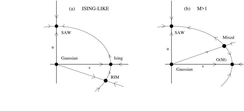
Figure 15: RG flow in the coupling plane $(u,v)$ for (a) Ising ($M=1$) and (b) $M$-component ($M>1$) randomly dilute systems.

In the RG approach one assumes that the replica symmetry is not broken. In recent years, however, this picture has been questioned [350, 349, 348] on the ground that the RG approach may not take into account other local minimum configurations of the random Hamiltonian (11.17), which may cause the spontaneous breaking of the replica symmetry. Arguments in favor of the stability of the critical behavior with respect to replica-symmetry breaking are reported in Ref. [934]. They consider an appropriate effective Hamiltonian allowing for possible replica-symmetry breaking terms and, using two-loop calculations, argue that the replica-symmetric FP is stable.

For generic values of $M$ and $N$, the Hamiltonian ${\cal H}_{MN}$ describes $M$ coupled $N$-vector models and it is usually called $MN$ model [16]. Figure 15 sketches the expected flow diagram for Ising ($M=1$) and multicomponent ($M>1$) systems in the limit $N\rightarrow 0$. There are four FP’s: the trivial Gaussian one, an O($M$)-symmetric FP, a self-avoiding walk (SAW) FP and a mixed FP. We recall that the region relevant for quenched disordered systems corresponds to negative values of the coupling $u$ [474, 26]. The SAW FP is stable and corresponds to the $(MN)$-vector theory for $N\rightarrow 0$, but it is not of interest for the critical behavior of randomly dilute spin models, since it is located in the region $u>0$. The stability of the other FP’s depends on the value of $M$. Nonperturbative arguments [968, 16] show that the stability of the O($M$) FP is related to the specific-heat critical exponent of the O($M$)-symmetric theory. Indeed, ${\cal H}_{MN}$ at the O($M$)-symmetric FP can be interpreted as the Hamiltonian of $N$ $M$-vector systems coupled by the O($MN$)-symmetric term. Since this interaction is the sum of the products of the energy operators of the different $M$-vector models, the crossover exponent associated with the O($MN$)-symmetric quartic interaction is given by the specific-heat critical exponent $\alpha_{M}$ of the $M$-vector model, independently of $N$. This implies that for $M=1$ (Ising-like systems) the pure Ising FP is unstable since $\phi=\alpha_{I}>0$, while for $M>1$ the O($M$) FP is stable given that $\alpha_{M}<0$, in agreement with the Harris criterion. For $M>1$ the mixed FP is in the region of positive $u$ and is unstable [16]. Therefore, the RG flow of the $M$-component model with $M>1$ is driven towards the pure O($M$) FP. Quenched disorder yields corrections to scaling proportional to the spin dilution and to $|t|^{\Delta_{r}}$ with $\Delta_{r}=-\alpha_{M}$. Note that, for the physically interesting two- and three-component models, the absolute value of $\alpha_{M}$ is very small: $\alpha_{2}\approx-0.014$ and $\alpha_{3}\approx-0.13$. Thus, disorder gives rise to very slowly-decaying scaling corrections. For Ising-like systems, the pure Ising FP is instead unstable, and the flow for negative values of the quartic coupling $u$ leads to the stable mixed or random FP which is located in the region of negative values of $u$. The above picture emerges clearly in the framework of the $\epsilon$ expansion, although the RIM FP is of order $\sqrt{\epsilon}$ [629] rather than $\epsilon$.

The Hamiltonian ${\cal H}_{MN}$ has been the object of several FT studies, especially for $M=1$ and $N=0$, the case that describes the RIM. In Table 35 we report a summary of the FT results obtained for the RIM universality class. Several computations have been done in the framework of the $\epsilon$ expansion and of the fixed-dimension $d=3$ expansion. Other results have been obtained by nonperturbative methods (CRG and scaling field) [1064, 835],

Table 35: FT estimates of the critical exponents for the RIM universality class. Here “$d=3$ exp” denotes the massive scheme in three dimensions, “$d=3$ MS” the minimal subtraction scheme without $\epsilon$ expansion. All perturbative results have been obtained by means of Padé-Borel or Chisholm-Borel resummations, except the results of Ref. [771] indicated by “$\epsilon$W” obtained using the $\epsilon$-algorithm of Wynn and of those of Ref. [908].

Ref.	Method	$\gamma$	$\nu$	$\eta$	$\alpha$	$\beta$	$\omega$
[908] 2000	$d=3$ exp $O(g^{6})$	1.330(17)	0.678(10)	0.030(3)	$-0.034(30)$	0.349(5)	0.25(10)
[874] 2000	$d=3$ exp $O(g^{5})$	1.325(3)	0.671(5)	0.025(10)	$-0.013(15)$	0.344(4)	0.32(6)
[436, 435] 2000	$d=3$ MS $O(g^{4})$	1.318	0.675	0.049	$-0.025$	0.354	0.39(4)
[1078] 2000	$d=3$ exp $O(g^{4})$	1.336(2)	0.681(12)	0.040(11)	$-0.043(36)$	0.354(7)	0.31
[771] 1989	$d=3$ exp $O(g^{4})$	1.321	0.671	0.031	$-0.013$	0.346
[771] 1989	$d=3$ exp $O(g^{4})$ $\epsilon$W	1.318	0.668	0.027	$-0.004$	0.343
[775] 1989	$d=3$ exp $O(g^{4})$	1.326	0.670	0.034	$-0.010$	0.346
[1064] 2002	CRG	1.306	0.67	0.05	$-0.01$	0.352
[835] 1982	scaling field		0.697		$-0.09$		0.42

The analysis of the FT expansions is made difficult by the more complicated analytic structure of the field theory corresponding to quenched disordered models. This issue has been investigated considering the free energy in zero dimensions. The large-order behavior of its double expansion in the quartic couplings $u$ and $v$, $F(u,v)=\sum_{ij}c_{ij}u^{i}v^{j}$, shows that the expansion in powers of $v$, keeping the ratio $u/v$ fixed, is not Borel summable [173]. As shown in Ref. [778], this a consequence of the fact that, because of the quenched average, there are additional singularities corresponding to the zeroes of the partition function $Z(\psi,g_{0})$ defined using the Hamiltonian (11.17). The problem is reconsidered in Ref. [37]. In the same context of the zero-dimensional model, it is shown that a more elaborate resummation can provide the correct determination of the free energy from its perturbative expansion. The procedure is still based on a Borel summation, which is performed in two steps: first, one writes $F(u,v)=\sum_{i}e_{i}(v)u^{i}$ where $e_{i}(v)=\sum_{j}c_{ij}v^{j}$ and resums the coefficient functions $e_{i}(v)$ of the series in $u$; then, one resums the resulting series in the coupling $u$. There is no proof that this procedure works also in higher dimensions, since the method relies on the fact that the zeroes of the partition function stay away from the real values of $v$. This is far from obvious in higher-dimensional systems.

The $MN$ model has been extensively studied in the framework of the $\epsilon$ expansion [509, 725, 629, 26, 474, 16, 475, 589, 1000, 834, 897, 320, 1007, 658, 1001]. Several studies also considered the equation of state [475, 834, 1007] and the two-point correlation function [475, 897]. In spite of these efforts, studies based on the $\epsilon$ expansion have not been able to go beyond a qualitative description of the physics of three-dimensional randomly dilute spin models. The $\sqrt{\epsilon}$ expansion [629] turns out not to be effective for a quantitative study of the RIM (see, e.g., the analysis of the five-loop series done in Ref. [1001]). The related minimal-subtraction renormalization scheme without $\epsilon$ expansion [984] have been also considered. The three-loop [584] and four-loop [434, 435, 436] results turn out to be in reasonable agreement with the estimates obtained by other methods. At five loops, however, no random FP is found [436] using this method. This negative result has been interpreted as a consequence of the non-Borel summability of the perturbative expansion. In this case, the four-loop series might represent the “optimal” truncation.

The most precise FT results have been obtained using the fixed-dimension expansion in $d=3$. Several quantities have been computed: the critical exponents [597, 773, 1006, 775, 771, 552, 553, 435, 1078, 874, 908], the equation of state [139], ratios of $n$-point susceptibilities in the HT phase [876], and the hyperuniversal ratio $R^{+}_{\xi}$ [139, 772]. The RG functions of the $MN$ model were calculated to six-loops in Ref. [908]. In the case relevant for the RIM universality class, i.e. $M=1$ and $N=0$, several methods of resummation have been applied. In Ref. [908] the method proposed in Ref. [37] was applied to the three-dimensional series. The analysis of the $\beta$-functions for the determination of the FP does not lead to a particularly accurate estimate of the random FP. Nonetheless, the RG functions associated with the exponents are largely insensitive to the exact position of the FP, so that accurate estimates of the critical exponents can still be obtained, see Table 35. Earlier analysis of the RIM series up to five-loops were done using Padé-Borel-Leroy approximants [874], thus assuming Borel summability. In spite of the fact that the series are not Borel summable, the results for the critical exponents turn out to be relatively stable, depending very little on the order of the series and the details of the analysis. They are in substantial agreement with the six-loop results of Ref. [908]. This fact may be explained by the observation of Ref. [173] that the Borel resummation applied in the standard way (i.e. at fixed $v/u$) may give a reasonably accurate result if one truncates the expansion at an appropriate point, i.e. for not too long series.

In conclusion, the agreement among FT results, experiments, and MC estimates is overall good. The FT method appears to have a good predictive power, in spite of the complicated analytic structure of the theory.

For $M\geq 2$ and $N=0$ the analysis of the corresponding six-loop series shows that no FP exists in the region $u<0$ and that the $O(M)$-symmetric FP is stable [908], in agreement with the Harris criterion.

Finally, we mention that the combined effect of cubic anisotropy and quenched uncorrelated impurities on multicomponent systems has been studied in Ref. [229].

11.5 Frustrated spin models with noncollinear order

Figure 16: The ground-state configuration of three $XY$ spins on a triangle coupled antiferromagnetically.

11.5.1 Physical relevance

The critical behavior of frustrated spin systems with noncollinear or canted order has been the object of intensive theoretical and experimental studies (see, e.g., Refs. [622, 299, 623] for recent reviews on this subject). Noncollinear order is due to frustration that may arise either because of the special geometry of the lattice, or from the competition of different kinds of interactions. Typical systems of the first type are three-dimensional stacked triangular antiferromagnets (STA’s), where magnetic ions are located at each site of a three-dimensional stacked triangular lattice. Examples are some ${\rm ABX}_{3}$-type compounds, where A denotes elements such as Cs and Rb, B is a magnetic ion such as Mn, Ni, and V, and X stands for halogens as Cl, Br, and I. Analogous behavior is observed in some BX₂ materials like VCl₂ and VBr₂. See Ref. [299] for a detailed description of the magnetic behavior of these materials. Frustration due to the competition of interactions may be realized in helimagnets, in which a magnetic spiral is formed along a certain direction of the lattice. The rare-earth metals Ho, Dy, and Tb provide physical examples of such systems.

All these systems are strongly anisotropic and the critical behavior is complex due to the competition between the $c$-axis coupling and the uniaxial anisotropy. Effective Hamiltonians describing the phase diagram of these compounds in a magnetic field are discussed in Refs. [919, 918, 917, 624, 621]. Mean-field and RG analyses predict several transition lines and the appearance of tetracritical and bicritical points, in good agreement with experiments.

The main point under discussion is the nature of the critical behavior. In particular, the question is whether along some transition lines or at the multicritical points one should observe a new chiral universality class, as originally conjectured by Kawamura [615, 616]. On this question, there is still much debate, FT methods, MC simulations, and experiments providing contradictory results in many cases.

11.5.2 Models

According to RG theory, the existence of a new (chiral) universality class may be investigated in simplified models retaining the basic features of the physical systems. One considers a three-dimensional stacked triangular lattice, which is obtained by stacking two-dimensional triangular layers, and the Hamiltonian

$${\cal H}_{\rm STA}=-J\,\sum_{\langle vw\rangle_{xy}}\vec{s}(v)\cdot\vec{s}(w)-J^{\prime}\,\sum_{\langle vw\rangle_{z}}\vec{s}(v)\cdot\vec{s}(w),$$ (11.20)

where $J<0$, the first sum is over nearest-neighbor pairs within the triangular layers ($xy$ planes), and the second one is over orthogonal interlayer nearest neighbors. The sign of $J^{\prime}$ is not relevant, since there is no frustration along the direction orthogonal to the triangular layers. The variables $\vec{s}$ are $N$-dimensional unit spins defined on the sites of the lattice; of course, $N=2$ and $N=3$ are the cases of physical relevance.

Triangular antiferromagnets are frustrated. Nonetheless, for $N\geq 2$ they admit an ordered ground state. For instance, for $N=2$ the ground state shows the 120^o structure of Fig. 16. There are two chirally degenerate configurations, according to whether the noncollinear spin configuration is right- or left-handed. The chiral degrees of freedom are related to the local quantity [618]

$$C_{ij}\propto\sum_{<vw>\in\vartriangle}\left[s_{i}(v)s_{j}(w)-s_{j}(v)s_{i}(w)\right],$$ (11.21)

where the summation runs over the three bonds of the given triangle.

Helimagnets can be modeled similarly. A simple model Hamiltonian is (see, e.g., Ref. [622])

$${\cal H}_{h}=-J_{1}\,\sum_{\langle ij\rangle_{nn}}\vec{s}_{i}\cdot\vec{s}_{j}-J_{2}\,\sum_{\langle ij\rangle_{nnn,z}}\vec{s}_{i}\cdot\vec{s}_{j},$$ (11.22)

where the first sum represents nearest-neighbor ferromagnetic interactions, so that $J_{1}>0$, while the second one describes antiferromagnetic next-nearest-neighbor interactions, i.e. $J_{2}<0$, along only one crystallografic axis $z$. In the LT phase, depending on the values of $J_{1}$ and $J_{2}$, competition of ferromagnetic and antiferromagnetic interactions may lead to incommensurate helical structures along the $z$-axis. The chiral degeneracy discussed in STA’s is also present in helimagnets.

On the basis of the structure of the ground state, one expects a breakdown of the symmetry from O$(N)$ in the HT phase to O$(N-2)$ in the LT phase. Therefore, the LGW Hamiltonian describing these systems must be characterized by a matrix order parameter. The determination of the effective Hamiltonian goes through fairly standard steps. One starts from the spin model (11.20), performs a Hubbard-Stratonovich transformation that allows to replace the fixed-length spins with variables of unconstrained length, expands around the instability points, and drops terms beyond quartic order [618]. One finally obtains the $O(N)\times O(M)$ symmetric Hamiltonian [618, 622]

$${\cal H}=\int d^{d}x\Bigl{\{}{1\over 2}\sum_{a}\Bigl{[}(\partial_{\mu}\phi_{a})^{2}+r\phi_{a}^{2}\Bigr{]}+{1\over 4!}u_{0}\Bigl{(}\sum_{a}\phi_{a}^{2}\Bigr{)}^{2}+{1\over 4!}v_{0}\sum_{a,b}\Bigl{[}(\phi_{a}\cdot\phi_{b})^{2}-\phi_{a}^{2}\phi_{b}^{2}\Bigr{]}\Bigr{\}},$$ (11.23)

where $\phi_{a}$ ($1\leq a\leq M$) are $M$ sets of $N$-component vectors. The case $M=2$ with $v_{0}>0$ describes frustrated systems with noncollinear ordering such as STA’s. Negative values of $v_{0}$ correspond to simple ferromagnetic or antiferromagnetic ordering, and to magnets with sinusoidal spin structures [618].

We mention a few other applications of the Hamiltonian (11.23). The superfluid phase of liquid ³He can be described by a field theory for complex 3$\times$3 matrices representing fermion pairs. Due to the magnetic dipole-dipole interaction that couples orbital momentum and spin, the superfluid order parameter is expected to have O(3)$\times$U(1) symmetry, which is the symmetry of the Hamiltonian (11.23) for $M=2$ and $N=3$. According to Refs. [593, 88], in the absence of an external magnetic field and neglecting the strain free-energy term, the transition from normal to planar superfluid is described by the effective LGW Hamiltonian (11.23) with $v_{0}<0$. The same LGW Hamiltonian, but with $v_{0}>0$, should describe the transition from normal to superfluid A₁ phase in the presence of a magnetic field [593, 88]. The model (11.23) can be also applied to the superconducting phase transition of heavy-fermion superconductors such as UPt₃ [596], and to the quantum phase transition of certain Josephson-junction arrays in a magnetic field [469] (see also Ref. [55] for a discussion of these systems). One may also consider more general O($N$)$\times$O($M$) models with $M>2$ [347, 619, 946, 755, 67, 622, 719, 1063]. In particular, the principal chiral model with $N=M=3$ may be relevant for magnets with noncollinear noncoplanar spin ordering.

In the following we only consider the $M=2$ case that is relevant for frustrated models with noncollinear order. In this case the LGW Hamiltonian (11.23) can also be written in terms of an $N$-component complex field $\psi$ as [55]

$${\cal H}=\int d^{d}x\left[{1\over 2}\left(\partial_{\mu}\psi^{*}\partial_{\mu}\psi+r\psi^{*}\psi\right)+{1\over 4!}y_{0}\left(\psi^{*}\cdot\psi\right)^{2}+{1\over 4!}w_{0}|\psi\cdot\psi|^{2}\right].$$ (11.24)

The couplings of the models (11.23) and (11.24) are related by $y_{0}=u_{0}-v_{0}/2$ and $w_{0}=v_{0}/2$. Note also that, for $N=2$, the transformation

$$\phi_{11}={\phi^{\prime}_{11}-\phi^{\prime}_{22}\over\sqrt{2}},\quad\phi_{12}={\phi^{\prime}_{12}-\phi^{\prime}_{21}\over\sqrt{2}},\quad\phi_{21}={\phi^{\prime}_{12}+\phi^{\prime}_{21}\over\sqrt{2}},\quad\phi_{22}={\phi^{\prime}_{11}+\phi^{\prime}_{22}\over\sqrt{2}},$$

$$\qquad u^{\prime}_{0}=u_{0}+v_{0}/2,\qquad v^{\prime}_{0}=-v_{0}$$ (11.25)

maps the chiral Hamiltonian (11.23) into the Hamiltonian (11.19) of the $MN$ model with $M=2$, $N=2$.

11.5.3 Theoretical results

Table 36: Theoretical estimates of the critical exponents for two- and three-component chiral systems. Results labeled MC have been obtained by means of Monte Carlo simulations, those labeled FT from the analysis of six-loop perturbative field-theoretic expansions in $d=3$.

	Ref.	Method	$\gamma$	$\nu$	$\beta$	$\alpha$	$\eta$
$N=2$	[901] 2000	FT	1.10(4)	0.57(3)	0.31(2)	0.29(9)	0.09(1)
	[1156] 2001	MC	1.074(13)	0.514(7)
	[169] 1996	MC	1.15(5)	0.48(2)	0.25(2)	0.46(10)
	[920] 1994	MC	1.03(4)	0.50(1)	0.24(2)	0.46(10)
	[620] 1992	MC	1.13(5)	0.54(2)	0.253(10)	0.34(6)
$N=3$	[901] 2000	FT	1.06(5)	0.55(3)	0.30(2)	0.35(9)	0.10(1)
	[146] 1994	MC	1.176(20)	0.585(9)	0.289(10)
	[756] 1994	MC	1.185(3)	0.586(8)	0.285(11)
	[721] 1994	MC	1.25(3)	0.59(1)	0.30(2)
	[620] 1992	MC	1.17(7)	0.59(2)	0.30(2)	0.24(8)

The critical behavior of frustrated systems with noncollinear order is quite controversial, since different theoretical methods, such as MC, CRG, and perturbative FT approaches provide contradictory results. Since all these approaches rely on different approximations and assumptions, their comparison and consistency is essential before considering the issue substantially understood.

Frustrated models with noncollinear order have been much studied using FT RG methods [80, 447, 88, 104, 1092, 617, 618, 67, 1158, 55, 57, 592, 724, 1060, 901, 225, 902, 1061, 903]. Two different expansion schemes have been used: the $\epsilon$ expansion and the fixed-dimension $d=3$ expansion.

A detailed discussion of the $\epsilon$-expansion results is presented in Ref. [622]. Near four dimensions, the $\epsilon$ expansion predicts four regimes. For $N>N_{+}$, there are four FP’s: the Gaussian FP, the $O(2N)$ FP, the XY FP and a mixed FP. The latter is the stable one and can be identified with the chiral FP. For $N_{-}<N<N_{+}$, only the Gaussian and the Heisenberg O($2N$)-symmetric FP’s are present, and none of them is stable. For $N_{H}<N<N_{-}$, there are again four FP’s, but none of them belongs to the physically relevant region $v_{0}>0$. For $N<N_{H}$, there are four FP’s, and the Heisenberg O$(2N)$-symmetric FP is the stable one. Three-loop calculations [57] give

$$N_{+}=21.80-23.43\epsilon+7.09\epsilon^{2}+O(\epsilon^{3}),$$

$$N_{-}=2.20-0.57\epsilon+0.99\epsilon^{2}+O(\epsilon^{3}),$$

$$N_{H}=2-\epsilon+1.29\epsilon^{2}+O(\epsilon^{3}).$$ (11.26)

Therefore, according to a “smooth extrapolation” of this scenario to three dimensions, the existence of chiral universality classes for $N=2,3$ requires $N_{+}<3$ in three dimensions. The analysis of the $\epsilon$ expansion of $N_{+}$ [55, 57, 901] shows that $N_{+}\approx 5$ in three dimensions. This estimate of $N_{+}$ is confirmed by CRG calculations, giving $N_{+}\approx 4$ [1060] and $N_{+}\approx 5$ [1061]. Therefore, there is a rather robust indication that $N_{+}>3$ in three dimensions, so that the stable chiral FP found near $d=4$ is not relevant for the three-dimensional physics of these systems.

On the other hand, one cannot exclude the existence of FP’s that are not smoothly connected with the FP’s described by the $\epsilon$ expansion. The investigation of such a possibility requires a strictly three-dimensional scheme. For both $N=2$ and $N=3$ cases, high-order calculations in the framework of the fixed-dimension $d=3$ expansion support the existence of a stable FP corresponding to the conjectured chiral universality class, and the RG flow diagram drawn in Fig. 17. Indeed, the six-loop analysis of Ref. [901] provides a rather robust evidence of their existence, contradicting earlier FT results based on three-loop series [55, 724]. In Ref. [226], on the basis of the six-loop fixed-dimension series, it has been argued that the stable chiral FP is actually a focus, essentially because the eigenvalues of its stability matrix turn out to be complex (only the positivity of their real part is required for the stability of the FP). The exponents at the chiral FP are given in Table 36. The major drawback of this computation is that the chiral FP lies in a region where the perturbative expansions are not Borel summable, although it is still within the region in which one can take into account the leading large-order behavior by a standard analysis based on a Borel transformation. Nevertheless, the observed stability of the results with the order of the series, from four to six loops, appears quite robust. We also mention that in the fixed-dimension approach, no FP is found for $5\mathrel{\hbox to0.0pt{\lower 3.0pt\hbox{$\mathchar 536\relax$}\hss}\raise 2.0pt\hbox{$\mathchar 316\relax$}}N\mathrel{\hbox to0.0pt{\lower 3.0pt\hbox{$\mathchar 536\relax$}\hss}\raise 2.0pt\hbox{$\mathchar 316\relax$}}7$, while for $N\mathrel{\hbox to0.0pt{\lower 3.0pt\hbox{$\mathchar 536\relax$}\hss}\raise 2.0pt\hbox{$\mathchar 318\relax$}}7$, a stable chiral FP is again present. These results may be interpreted as follows. The stable FP found for $N\mathrel{\hbox to0.0pt{\lower 3.0pt\hbox{$\mathchar 536\relax$}\hss}\raise 2.0pt\hbox{$\mathchar 318\relax$}}7$ is smoothly related to the large-$N$ and small-$\epsilon$ chiral FP. Such a FP disappears for $5\mathrel{\hbox to0.0pt{\lower 3.0pt\hbox{$\mathchar 536\relax$}\hss}\raise 2.0pt\hbox{$\mathchar 316\relax$}}N\mathrel{\hbox to0.0pt{\lower 3.0pt\hbox{$\mathchar 536\relax$}\hss}\raise 2.0pt\hbox{$\mathchar 316\relax$}}7$, so that we can identify $5\mathrel{\hbox to0.0pt{\lower 3.0pt\hbox{$\mathchar 536\relax$}\hss}\raise 2.0pt\hbox{$\mathchar 316\relax$}}N_{+}\mathrel{\hbox to0.0pt{\lower 3.0pt\hbox{$\mathchar 536\relax$}\hss}\raise 2.0pt\hbox{$\mathchar 316\relax$}}7$, in agreement with the above-reported estimates. According to the $\epsilon$-expansion scenario, for $N<N_{+}$ no stable FP’s should be found. However, the existence of a stable chiral FP for $N=2,3$ indicates that the situation is more complex in three dimensions: another value $3<N_{d3}<N_{+}$ exists such that, for $N<N_{d3}$, the system shows again a chiral critical behavior with a FP unrelated to the small-$\epsilon$ and large-$N$ chiral FP.

The new chiral FP’s found for $N=2,3$ should describe the apparently continuous transitions observed in $XY$ and Heisenberg chiral systems. Note that the presence of a stable FP does not exclude the possibility that some systems undergo a first-order transition. Symmetry arguments are not sufficient to establish the order of the transition. Indeed, within the RG approach, first-order transitions are still possible for systems that are outside the attraction domain of the chiral FP. In this case, the RG flow would run away to a first-order transition. This means that, even if some systems show a universal continuous transition related to the presence of a stable FP, other systems may exhibit a first-order transition. The different behavior of these systems is not due to the symmetry, but arises from the particular values of the microscopic parameters, which may be or not be in the attraction domain of the stable FP.

Figure 17: RG flow in the $(u,v)$ plane for $N=2,3$.

Studies based on approximate solutions of continuous RG equations (CRG) [1158, 1060, 1061, 1062] favor a weak first-order transition, since no evidence of stable FP’s has been found. In this scenario, the transition should be weak enough to effectively appear as continuous in experimental works. The weakness of the transition is somehow supported by the observation of a range of parameters in which the RG flow appears very slow, with effective critical exponents close to those found in experiments, for instance $\nu=0.53$, $\gamma=1.03$, $\beta=0.28$ for $N=3$. Note however that, as already discussed in Sec. 2.4.4, the practical implementation of CRG methods requires approximations and/or truncations of the effective action. Ref. [1158] employed a local potential approximation (LPA); Ref. [1060] used a more refined approximation that allows for an anomalous scaling of the field and therefore for a nontrivial value of $\eta$ (ILPA); finally, Ref. [1062] mentioned some attempts for a partial first-order derivative expansion approximation. These approximations are essentially limited to the lowest orders of the derivative expansion, so that their results may not be conclusive.

Also MC simulations (see, e.g., Refs. [615, 616, 338, 620, 678, 756, 920, 721, 146, 341, 169, 719, 722, 723, 564, 1156, 1157]) have not been conclusive in setting the question. Most simulations of the STA Hamiltonian observe second-order phase transitions. Some results are reported in Table 36. We observe small differences among the results of the MC simulations and the FT approach. Moreover, some MC results are not consistent with general exponent inequalities. Indeed, one must have $\eta\geq 0$, which follows from the unitarity of the corresponding quantum field theory [889, 1152] (one may show that the model (11.15) is reflection positive and thus the corresponding field theory is unitary). Using $\gamma=(2-\eta)\nu$ and $\beta={1\over 2}\nu(1+\eta)$, we obtain the inequalities $\gamma\leq 2\nu$ and $\beta\geq{1\over 2}\nu$. As it can be seen from the results of Table 36, the first inequality is not satisfied by the results of Refs. [169, 721, 1156], while the second one is barely satisfied by the results of Ref. [620]. This fact has been interpreted as an additional indication in favor of the first-order transition hypothesis [723, 724]. But, it may also be explained by sizeable scaling corrections, that are neglected in all these numerical studies. Ref. [564] reports simulations of various systems, and in particular STA spin systems. The results favor a first-order transition, although the evidence that the asymptotic critical behavior has been probed is not clear. We should also say that distinguishing a weak first-order transition from a continuous one is in general a hard task in numerical simulations. First-order transitions have been clearly observed in MC investigations [722, 723] of modified lattice spin systems that, according to general universality ideas, should belong to the same universality class of the Hamiltonian (11.20). But, as we already said, this does not necessarily contradict the existence of a stable FP. Indeed, mean-field arguments suggest a first-order transition for such modified systems [622].

Also higher values of $N$ have been studied, although they are not of physical interest. For $N=6$, MC simulations [724] and CRG calculations [1060] provide evidence for a second-order phase transition, showing also a good agreement in the estimates of the critical exponents.

We finally mention that in the many-component limit $N\rightarrow\infty$ at fixed $M$, the O($M$)$\times$O($N$) theory can be expanded in powers of $1/N$ [618, 622]. In the $1/N$-expansion the transition in the noncollinear case, i.e. for $v>0$, is continuous, and the exponents have been computed to $O(1/N^{2})$ [902, 618]. For $d=3$ and $M=2$ the critical exponents are given by

$$\hskip-22.76228pt\nu=1-{16\over\pi^{2}}{1\over N}-\left({56\over\pi^{2}}-{640\over 3\pi^{4}}\right){1\over N^{2}}+O\left({1\over N^{3}}\right),$$

$$\hskip-22.76228pt\eta={4\over\pi^{2}}{1\over N}-{64\over 3\pi^{4}}{1\over N^{2}}+O\left({1\over N^{3}}\right).$$ (11.27)

11.5.4 Experimental results

Table 37: Experimental estimates of the critical exponents for two- and three-component systems. We report results for stacked triangular antiferromagnets (STA) and helimagnets (HM).

	Material	$\gamma$	$\nu$	$\beta$	$\alpha$
$N=2$	CsMnBr3	1.10(5) [602]	0.57(3) [602]	0.25(1) [602]	0.39(9) [1098]
STA		1.01(8) [769]	0.54(3) [769]	0.21(2) [769]	0.36(4) [1098]
				0.24(2) [452]	0.40(5) [337]
				0.22(2) [768]
	RbMnBr3			0.28(2) [609]
	CsNiCl3			0.243(5) [371]	0.37(8)[116]
					0.342(5)[370]
	CsMnI3				0.34(6)[116]
$N=2$	Ho	1.24(15) [745]	0.57(4) [451]	0.37(10) [1055, 1056]	0.34(1) [590]
HM		1.14(10) [451]	0.54(4) [1056]	0.327 [1059]	0.27(2) [590]
				0.41(4) [535]	0.10(2) [1098]
				0.39(4) [535]	0.22(2) [1098]
				0.39(2) [359]
				0.38(1) [916]
	Dy	1.05(7) [451]	0.57(5) [451]	0.39(1) [189]	0.18(2) [691]
				0.38(2) [359]	0.16(1) [590]
$N=3$	VCl2	1.05(3) [603]	0.62(5) [603]	0.20(2) [603]
STA	VBr2				0.30(5) [1134]
	RbNiCl3			0.28(1) [864]
	CsNiCl3			0.28(3) [371]	0.25(8) [116]
					0.23(4) [370]
	CsMnBr3				0.28(6) [1101]
					0.44 [370]
	CsMn(Br0.19I0.81)3				0.23(7) [205]

For a critical discussion of the experimental results we refer to Refs. [299, 359, 622]. As already mentioned, on the basis of symmetry, one expects two classes of systems to have a similar behavior: STA’s and helimagnets. Apparently, all these systems show continuous phase transitions with the exception of CsCuCl₃. Experimental results are reported in Table 37. It is not a complete list, but it gives an overview of the experimental state of the art. Additional results are reported in Refs. [299, 359, 622].

Overall, experiments on STA’s favor a continuous transition belonging to a new chiral universality class. The measured critical exponents are in satisfactory agreement with the theoretical results of Table 36. However, as some MC results, the experimental estimates do not apparently satisfy the inequality $\beta\geq{1\over 2}\nu$. This fact could be explained by the presence of scaling corrections that are not considered in most of the experimental analyses. Of course, another possible explanation [1158, 1060, 1061, 1062] is that no chiral universality class exists, so that the transitions are weakly first-order ones and the measured exponents are simply effective.

The behavior of helimagnets is even more controversial. The estimates of the exponent $\beta$ are substantially larger than the experimental results for STA’s and also than the theoretical results of Table 36. But, as discussed in Ref. [622], special care should be taken in extracting information on the asymptotic critical behavior of rare-earth metals, essentially due to the more complicated physical mechanism that gives rise to the effective model (11.22) for helimagnets. Apart from the explanation in terms of a weak first-order transition, it is also possible that experiments have not really probed the asymptotic regime. For a discussion, see, e.g., Ref. [622]. Another possibility is that the current modelling of these systems becomes invalid near the critical point. There could be other interactions that are quantitatively small, but still change the asymptotic critical behavior of these systems. In both cases, one would be observing a crossover between different regimes.

11.5.5 Chiral crossover exponents

In the standard $O(N)$ model there is only one crossover exponent at quadratic order, which is associated with the spin-2 operator defined in Sec. (1.5.8). In the $O(M)\times O(N)$ model, there are four different quadratic operators [618, 622]. Two of them are particularly relevant, those associated with chirality and with the uniform anisotropy. Correspondingly, we define chirality exponents $\phi_{c}$, $\gamma_{c}$, and $\beta_{c}$, and anisotropy exponents $\phi_{a}$, $\gamma_{a}$, and $\beta_{a}$. These exponents are not independent: they are related by the relations (1.121).

The chirality exponents are associated with the operator (11.21), or in the FT framework, with the operator

$$C_{cd,kl}(x)=\phi_{ck}(x)\phi_{dl}(x)-\phi_{cl}(x)\phi_{dk}(x).$$ (11.28)

For $N=2$, there are several theoretical estimates. The analysis of six-loop perturbative series in the framework of the fixed-dimension expansion [903] gives $\phi_{c}=1.43(4)$, $\beta_{c}=0.28(10)$. MC simulations give: $\beta_{c}=0.45(2)$, $\gamma_{c}=0.77(5)$, $\phi_{c}=1.22(6)$ [620]; $\beta_{c}=0.38(2)$, $\gamma_{c}=0.90(9)$, $\phi_{c}=1.28(10)$ [920]; $\gamma_{c}=0.81(3)$ [1157]. The agreement is satisfactory, keeping into account the different systematic errors of the various approaches. Such exponents have been recently measured in Refs. [915, 916]. For the $XY$ STA CsMnBr₃, it was found [915] $\phi_{c}=1.28(7)$, $\beta_{c}=0.44(2)$, measured respectively in the HT and LT phases. These results are in reasonable agreement with the theoretical ones for the XY chiral universality class. On the other hand, for the helimagnet holmium it was found [916] $\beta_{c}=0.90(3)$, $\gamma_{c}=0.68(6)$, which are sensibly different from the theoretical results. Again, the reason for this discrepancy is unclear.

For $N=3$ only theoretical estimates are available: perturbative FT gives $\phi_{c}=1.27(4)$, $\beta_{c}=0.38(10)$ [903], while MC simulations give $\beta_{c}=0.55(4)$, $\gamma_{c}=0.72(8)$, $\phi_{c}=1.27(9)$ from Ref. [620] and $\beta_{c}=0.50(2)$ $\gamma_{c}=0.82(4)$ and $\phi_{c}=1.32(5)$ from Ref. [756].

An important question is the relevance of the $\mathbb{Z}_{2}$ chiral symmetry for the critical behavior of these systems. The experimental results of Ref. [915] show that chiral order and spin order occur simultaneously. Still, one may wonder whether the absence of the $\mathbb{Z}_{2}$-symmetry changes the critical behavior of these systems. In this respect, the results of Ref. [1156] are interesting. They considered two-dimensional spins on a stacked triangular lattice and the biquadratic Hamiltonian

$${\cal H}=-J\sum_{\langle ij\rangle}\left(\vec{s}_{i}\cdot\vec{s}_{j}\right)^{2},$$ (11.29)

with $J<0$. Because of the $\mathbb{Z}_{2}$ gauge symmetry $\vec{s}_{i}\to-\vec{s}_{i}$, chirality is identically zero. Nonetheless, the system shows a continuous transition with critical exponents $\gamma=1.072(9)$, $\nu=0.520(3)$, that are clearly compatible with the $XY$ chiral exponents, but again they do not satisfy the relation $\gamma<2\nu$. These results would suggest that frustration, not chirality, is the relevant ingredient characterizing the phase transition.

The anisotropy exponent $\phi_{a}$ describes the crossover near multicritical points in the presence of a magnetic field. Experimental results are discussed in Ref. [622].

11.6 The tetragonal Landau-Ginzburg-Wilson Hamiltonian

In this section we study the critical behavior of statistical systems that are described by the three-coupling LGW Hamiltonian

$${\cal H}=\int d^{d}x\Bigl{\{}\sum_{i,a}{1\over 2}\left[(\partial_{\mu}\phi_{a,i})^{2}+r\phi_{a,i}^{2}\right]+\sum_{ij,ab}{1\over 4!}\left(u_{0}+v_{0}\delta_{ij}+w_{0}\delta_{ij}\delta_{ab}\right)\phi^{2}_{a,i}\phi^{2}_{b,j}\Bigr{\}},$$ (11.30)

where $a,b=1,...M$ and $i,j=1,...N$. Note that, as particular cases, one may recover the $MN$ model, for $w_{0}=0$, the $(M\times N$)-component model with cubic anisotropy for $v_{0}=0$, and $N$ decoupled $M$-component cubic models for $u_{0}=0$. The models with $M=2$ are physically interesting: They should describe the critical properties in some structural and antiferromagnetic phase transitions [812, 813, 829, 16, 814, 815, 80, 478, 986, 1065]. Therefore, we will restrict ourselves to the case $M=2$. In the following the Hamiltonian (11.30) with $M=2$ will be named tetragonal.

We mention that in the literature the tetragonal Hamiltonian is also written in terms of a $2N$-component vector field $\varphi_{i}$:

$${\cal H}=\int d^{d}x\Bigl{\{}{1\over 2}\sum_{i=1}^{2N}\left[(\partial_{\mu}\varphi_{i})^{2}+r\varphi_{i}^{2}\right]+{1\over 4!}z_{1}(\sum_{i=1}^{2N}\varphi_{i}^{2})^{2}+{1\over 4!}z_{2}\sum_{i=1}^{2N}\varphi_{i}^{4}+{1\over 4!}2z_{3}\sum_{j=1}^{N}\varphi_{2j-1}^{2}\varphi_{2j}^{2}\Bigr{\}}.$$ (11.31)

The relations between the two sets of couplings are $z_{1}=u_{0}$, $z_{2}=v_{0}+w_{0}$, and $z_{3}=v_{0}$.

Note that the tetragonal Hamiltonian is symmetric under the transformation [667]

$$(\phi_{1,i}\;,\;\phi_{2,i}) \longrightarrow {1\over\sqrt{2}}(\phi_{1,i}+\phi_{2,i}\;,\;\phi_{1,i}-\phi_{2,i}),$$

$$(u_{0},v_{0},w_{0}) \longrightarrow (u_{0},v_{0}+{\textstyle\frac{3}{2}}w_{0},-w_{0}).$$ (11.32)

Many physical systems are expected to be described by the tetragonal Hamiltonian. Indeed, for $N=2$ the tetragonal Hamiltonian should be relevant for the structural phase transition in NbO₂ and, for $w_{0}=0$, for the antiferromagnetic transitions in TbAu₂ and DyC₂. The case $N=3$ describes the antiferromagnetic phase transitions in the K₂IrCl₆ crystal and, for $w_{0}=0$, those in TbD₂ and Nd. Experimental results show continuous phase transitions in all the above-mentioned cases (see, e.g., Ref. [1065] and references therein).

The $\epsilon$ expansion analysis of the tetragonal Hamiltonian indicates the presence of eight FP’s [812, 813, 814]. In order to understand their physical properties, we begin by discussing the special cases when one of the couplings is zero. As already mentioned, for $u=0$ the model is equivalent to $N$ decoupled cubic models with two-component spins, while for $v=0$ the model is equivalent to a cubic model with $2N$-component spins. Since $N$ is supposed to be larger than one, using the results reported in Sec. 11.3, we conclude that in the plane $u=0$ the stable FP is the $XY$ one, and the cubic and the Ising FP’s are equivalent because they can be related through the symmetry (11.32). On the other hand, in the plane $v=0$ the stable FP is the cubic one. Figure 18 shows sketches of the flow diagram in the two planes $u=0$ and $v=0$.

Figure 18: RG flow in the planes $u=0$ and $v=0$.

In the case $w=0$ the tetragonal Hamiltonian describes $N$ coupled $XY$ models. Such theories have four FP’s [178, 16]: the trivial Gaussian one, the $XY$ one where the $N$ $XY$ models decouple, the O($2N$)-symmetric and the mixed tetragonal FP’s. The Gaussian one is again never stable. One can argue that, at the $XY$ FP, the crossover exponent related to the O($2N$)-symmetric interaction is given by $\phi=\alpha_{XY}$ [968, 16, 306], where $\alpha_{XY}$ is the specific heat exponent of the $XY$ model. This result is again based on the observation that when $w=0$ the tetragonal Hamiltonian describes $N$ interacting $XY$ models, and the O($2N$)-symmetric interaction can be represented as the product of two energy operators of the $XY$ subsystems [968]. Since $\alpha_{XY}$ is negative, the $XY$ FP should be stable with respect to the O($2N$)-symmetric interaction. In turn, one expects that the O($2N$)-symmetric and the tetragonal FP’s are unstable. The resulting sketch of the RG flow in the plane $w=0$ is given by the case (A) of Fig. 19.

Figure 19: Two possibilities for the RG flow in the plane $w=0$.

We have so identified seven out of eight FP’s. The eighth one can be obtained by applying the transformation (11.32) to the cubic FP lying in the $v_{0}=0$ plane.

Therefore, the above-reported analysis leaves us with three possible stable FP points: the cubic one in the $v=0$ plane and its symmetric counterpart, and the $XY$ FP with $u=w=0$. The cubic FP, which is stable in the $v=0$ plane, turns out to be unstable with respect to the quartic interaction associated with the coupling $v$. This is clearly seen from the analyses of both the $\epsilon$ and the fixed-dimension expansions. Of course, also its symmetric counterpart is unstable and therefore, the $XY$ FP is the only—at least among the FP’s predicted by the $\epsilon$ expansion—stable FP of the tetragonal theory, independently of the value of $N$. Thus, systems described by the tetragonal Hamitonian are expected to have $XY$ critical behavior.

The global stability of the $XY$ FP has been apparently contradicted by FT studies. The analysis of the two-loop $\epsilon$ expansion [812, 813, 814] predicts a globally stable tetragonal FP, which is the one in the plane $w=0$, and an unstable $XY$ FP. In the plane $w=0$, the predicted RG flow is given by case (B) of Fig. 19. This fact should not come unexpected because $\alpha_{XY}=\epsilon/10+O(\epsilon^{2})$, so that, according to the arguments of Refs. [968, 16, 306], sufficiently close to $d=4$ the FP describing $N$ decoupled $XY$ models is unstable and the tetragonal FP dominates the critical behavior. However, in order to obtain reliable results in three dimensions from the $\epsilon$ expansion, higher-order calculations with a proper resummation of the series are necessary.

The RG flow (B) of Fig. 19 is further supported by recent higher-loop calculations. The stability of the tetragonal FP has been confirmed by calculations up to $O(\epsilon^{4})$ in the framework of the $\epsilon$-expansion [811, 808, 320]. The same result has been obtained by a Padè-Borel analysis of the three-loop series in the framework of the fixed-dimension expansion [1024, 1006]. However, we mention that the authors of Ref. [1024], noting the closeness of the apparently stable tetragonal and unstable $XY$ FP’s, argued that the respective stability-instability may be a misleading effect of the relatively few terms of the series.

In order to clarify this issue, we have extended the fixed-dimension expansion of the tetragonal Hamiltonian to six loops. Note that, since the tetragonal model for $w_{0}=0$ is nothing but the $MN$ model with $M=2$, the results of Sec. 11.5 show that, at least for $N=2$, there is another stable FP in the region $v<0$, whose presence is not predicted by the $\epsilon$ expansion. In the following we will not investigate this issue, although it would be worthwhile to perform a more systematic study, but we will only focus on the stability properties of the $XY$ FP.

The tetragonal FT theory is renormalized by introducing a set of zero-momentum conditions for the one-particle irreducible two-point and four-point correlation functions, such as Eq. (11.3) and

$$\Gamma^{(4)}_{ai,bj,ck,dl}(0)=mZ_{\phi}^{-2}\left(uA_{ai,bj,ck,dl}+vB_{ai,bj,ck,dl}+wC_{ai,bj,ck,dl}\right)$$ (11.33)

where, setting $\delta_{ai,bj}\equiv\delta_{ab}\delta_{ij}$,

$$A_{ai,bj,ck,dl}={\textstyle\frac{1}{3}}\left(\delta_{ai,bj}\delta_{ck,dl}+\delta_{ai,ck}\delta_{bj,dl}+\delta_{ai,dl}\delta_{bj,ck}\right),$$

$$B_{ai,bj,ck,dl}=\delta_{ij}\delta_{ik}\delta_{il}\,{\textstyle\frac{1}{3}}\left(\delta_{ab}\delta_{cd}+\delta_{ac}\delta_{bd}+\delta_{ad}\delta_{bc}\right),$$

$$C_{ai,bj,ck,dl}=\delta_{ij}\delta_{ik}\delta_{il}\,\delta_{ab}\delta_{ac}\delta_{ad}.$$ (11.34)

The mass $m$, and the zero-momentum quartic couplings $u$, $v$, and $w$ are related to the corresponding Hamiltonian parameters by

$$u_{0}=muZ_{u}Z_{\phi}^{-2},\qquad v_{0}=mvZ_{v}Z_{\phi}^{-2},\qquad w_{0}=mwZ_{w}Z_{\phi}^{-2}.$$ (11.35)

The FP’s of the theory are given by the common zeros of the $\beta$-functions $\beta_{u}(u,v,w)$, $\beta_{v}(u,v,w)$, and $\beta_{w}(u,v,w)$, associated with the couplings $u$, $v$, and $w$ respectively. Their stability properties are controlled by the matrix

$$\Omega=\left(\matrix{\frac{\partial\beta_{u}}{\partial u}&\frac{\partial\beta_{u}}{\partial v}&\frac{\partial\beta_{u}}{\partial w}\cr\frac{\partial\beta_{v}}{\partial u}&\frac{\partial\beta_{v}}{\partial v}&\frac{\partial\beta_{v}}{\partial w}\cr\frac{\partial\beta_{w}}{\partial u}&\frac{\partial\beta_{w}}{\partial v}&\frac{\partial\beta_{w}}{\partial w}}\right)\;.$$ (11.36)

We have computed the perturbative expansion of the two-point and four-point correlation functions to six loops. The diagrams contributing to this calculations are approximately 1000. We handled them with a symbolic manipulation program, which generates the diagrams and computes the symmetry and group factors of each of them. We did not calculate the integrals associated with each diagram, but we used the numerical results compiled in Ref. [843]. Summing all contributions, we determined the RG functions to six loops. We report our results in terms of the rescaled couplings

$$u\equiv{16\pi\over 3}R_{2N}\bar{u},\qquad v\equiv{16\pi\over 3}R_{2}\bar{v},\qquad w\equiv{16\pi\over 3}\bar{w},$$ (11.37)

where $R_{K}=9/(8+K)$. The resulting series are

$$\beta_{\bar{u}}=-\bar{u}+\bar{u}^{2}+{4\over 5}\bar{u}\bar{v}+{2\over 3}\bar{u}\bar{w}-{2(95+41N)\over 27(4+N)^{2}}\bar{u}^{3}-{80\over 27(4+N)}\bar{u}^{2}\bar{v}-{200\over 81(4+N)}\bar{u}^{2}\bar{w}$$

$$-{92\over 675}\bar{u}\bar{v}^{2}-{92\over 729}\bar{u}\bar{w}^{2}-{92\over 405}\bar{u}\bar{v}\bar{w}+\bar{u}\;(\sum_{i+j+k\geq 3}b^{(u)}_{ijk}\;\bar{u}^{i}\bar{v}^{j}\bar{w}^{k}),$$ (11.38)

$$\beta_{\bar{v}}=-\bar{v}+\bar{v}^{2}+{6\over 4+N}\bar{u}\bar{v}+{2\over 3}\bar{v}\bar{w}-{272\over 675}\bar{v}^{3}-{724\over 135(4+N)}\bar{u}\bar{v}^{2}-{2(185+23N)\over 27(4+N)^{2}}\bar{u}^{2}\bar{v}$$

$$-{40\over 81}\bar{v}^{2}\bar{w}-{92\over 729}\bar{v}\bar{w}^{2}-{308\over 81(4+N)}\bar{u}\bar{v}\bar{w}+\bar{v}\;(\sum_{i+j+k\geq 3}b^{(v)}_{ijk}\;\bar{u}^{i}\bar{v}^{j}\bar{w}^{k}),$$ (11.39)

$$\beta_{\bar{w}}=-\bar{w}+\bar{w}^{2}++{6\over 4+N}\bar{u}\bar{w}+{6\over 5}\bar{v}\bar{w}-{308\over 729}\bar{w}^{3}-{416\over 81(4+N)}\bar{u}\bar{w}^{2}-{416\over 405}\bar{v}\bar{w}^{2}$$

$$-{2(185+23N)\over 27(4+N)^{2}}\bar{u}^{2}\bar{w}-{416\over 675}\bar{v}^{2}\bar{w}-{832\over 135(4+N)}\bar{u}\bar{v}\bar{w}+\bar{w}\;(\sum_{i+j+k\geq 3}b^{(w)}_{ijk}\;\bar{u}^{i}\bar{v}^{j}\bar{w}^{k}).$$ (11.40)

The coefficients $b^{(u)}_{ijk}$, $b^{(v)}_{ijk}$, $b^{(w)}_{ijk}$, with $3\leq i+j+k\leq 6$ are reported in the Tables 38, 39, and 40, respectively.

We report the RG functions $\eta_{\phi}$ and $\eta_{t}$ to two loops only (the complete six-loop series are available on request), since we will not use them in our analysis. They are

$$\eta_{\phi} = {4(1+N)\over 27(4+N)^{2}}\bar{u}^{2}+{16\over 135(4+N)}\bar{u}\bar{v}+{8\over 81(4+N)}\bar{u}\bar{w}+{8\over 675}\bar{v}^{2}+{8\over 405}\bar{v}\bar{w}+{8\over 729}\bar{w}^{2}+...$$ (11.41)

$$\eta_{t} = -{1+N\over 4+N}\bar{u}-{2\over 5}\bar{v}-{1\over 3}\bar{w}+{1+N\over(4+N)^{2}}\bar{u}^{2}+{4\over 5(4+N)}\bar{u}\bar{v}+{2\over 25}\bar{v}^{2}+{2\over 3(4+N)}\bar{u}\bar{w}$$ (11.42)

$$+{4\over 30}\bar{v}\bar{w}+{2\over 27}\bar{w}^{2}+...$$

In the following we limit ourselves to check the stability of the $XY$ FP, whose coordinates are $\overline{u}^{*}=0$, $\overline{v}_{XY}^{*}=1.402(4)$ [233, 481], and $\overline{w}^{*}=0$. One can easily see that the eigenvalues of the stability matrix (11.36) at the $XY$ FP are given simply by

$$\omega_{1}={\partial\beta_{\overline{u}}\over\partial\overline{u}}(0,\overline{v}_{XY}^{*},0),\qquad\omega_{2}={\partial\beta_{\overline{v}}\over\partial\overline{v}}(0,\overline{v}_{XY}^{*},0),\qquad\omega_{3}={\partial\beta_{\overline{w}}\over\partial\overline{w}}(0,\overline{v}_{XY}^{*},0).$$ (11.43)

Note that $\omega_{i}$ are $N$-independent, as it can be checked by looking at the corresponding series. According to the nonpertubative argument reported above, the $XY$ FP is stable, and the smallest eigenvalue of the stability matrix $\Omega$ should be given by

$$\omega_{1}=-{\alpha_{XY}\over\nu_{XY}},$$ (11.44)

where $\alpha_{XY}$ and $\nu_{XY}$ are the critical exponents of the $XY$ model. In the analysis we exploit the knowledge of the large-order behavior of the series, which is determined by the $XY$ FP only and therefore it is the same as the one of the O(2)-symmetric theory. We skip the details, since the analysis is identical to that performed in Ref. [908] to study the stability of the O($M$)-symmetric FP in the $MN$ model. Our estimate is

$$\omega_{1}=0.007(8).$$ (11.45)

The stability of the $XY$ FP is substantially confirmed, although the apparent error of the analysis does not completely exclude the opposite sign for $\omega_{1}$. The estimate of $\omega_{1}$ turns out to be substantially consistent with the value one obtains using Eq. (11.44). Indeed, $\alpha_{XY}/\nu_{XY}=-0.0217(12)$ using the recent estimates of the $XY$ critical exponents of Ref. [233], and $\alpha_{XY}/\nu_{XY}=-0.016(7)$ and $\alpha_{XY}/\nu_{XY}=-0.010(9)$ using the estimates respectively of Ref. [481] and [693] that were obtained by a more similar technique, i.e. from the analysis of the fixed-dimension expansion of the O(2)-symmetric model. It is easy to see that $\omega_{3}$ is equal to the smallest eigenvalue of stability matrix of the two-component cubic model at the $XY$ FP, see Sec. 11.3, thus $\omega_{3}=0.103(8)$. The eigenvalue $\omega_{2}$ is the one determining the leading scaling corrections in the $XY$ model and it is given by $\omega_{2}=0.789(11)$  [481].

In conclusion the analysis of the six-loop fixed-dimension expansion turns out to be substantially consistent with the nonperturbative prediction indicating that the $XY$ FP is globally stable independently of $N$.

11.7 LGW Hamiltonian with symmetry O$(n_{1})\oplus$O$(n_{2})$ and multicritical phenomena

We now consider an $N$-component system with symmetry O$(n_{1})\oplus$O$(n_{2})$ with $n_{1}+n_{2}=N$. The most general Hamiltonian containing up to quartic terms is given by [913, 407, 669]

$${\cal H}=\int d^{3}x\Bigl{[}{\textstyle\frac{1}{2}}(\partial_{\mu}\phi_{1})^{2}+{\textstyle\frac{1}{2}}(\partial_{\mu}\phi_{2})^{2}+{\textstyle\frac{1}{2}}r_{1}\phi_{1}^{2}+{\textstyle\frac{1}{2}}r_{2}\phi_{2}^{2}+u_{1}(\phi_{1}^{2})^{2}+u_{2}(\phi_{2}^{2})^{2}+w\phi_{1}^{2}\phi_{2}^{2}\Bigr{]},$$ (11.46)

where $\phi_{1}$, $\phi_{2}$ are $n_{1}$-, $n_{2}$-component fields with $n_{1}+n_{2}=N$. We are interested in the critical behavior at the multicritical point, where two critical lines with O$(n_{1})$ and O$(n_{2})$ symmetry meet. For this purpose, one must analyze the FP’s of the theory when both $r_{1}$ and $r_{2}$ are tuned to their critical value. According to the $O(\epsilon)$ analysis of Ref. [669] (see also Ref. [19]) the model has six FP’s. Three of them, i.e. the Gaussian, the O($n_{1}$) and the O($n_{2}$) FP’s, are always unstable. The other three FP’s are the bicritical $O(N)$-symmetric FP, and the tetracritical decoupled and biconal FP’s. The stability of these FP’s depends on $n_{1}$ and $n_{2}$. For the decoupled FP, one can use nonperturbative arguments to establish its stability properties with respect to the $w$-interaction [19]. The RG dimension $y_{w}$ of the operator $w\phi_{1}^{2}\phi_{2}^{2}$ that couples the two fields $\phi_{1}$ and $\phi_{2}$ is given by

$$y_{w}={\alpha_{1}\over 2\nu_{1}}+{\alpha_{2}\over 2\nu_{2}},$$ (11.47)

where $\alpha_{i}$ and $\nu_{i}$ are the critical exponents of the O$(n_{i})$ theory. For $n_{1}\geq 2$ and $n_{2}\geq 2$, we have $\alpha_{i}<0$, so that $y_{w}<0$. Therefore, the perturbation is irrelevant and the decoupled FP is stable. For $n_{1}=1$, the perturbation is irrelevant for $\nu_{2}>\nu_{I}/(3\nu_{I}-1)\approx 0.7077(2)$, where we have used the estimate of $\nu_{I}$ of Ref. [243]. Therefore, the decoupled FP is stable for $n_{2}\geq 3$ and unstable for $n_{2}=1,2$.

In order to study the stability properties of the bicritical O($N$) FP, we consider generic O($n_{1}$)$\oplus$O($n_{2}$) invariant perturbations ${\cal P}_{ml}$ at the O($N$)-summetric FP, where $m$ is the power of the fields and $l$ the spin of the representation of the O($N$) group [230]. For $m=2$ (resp. 4), the only possible values of $l$ are $l=0,2$ (resp. $l=0,2,4$). Explicitly,

$${\cal P}_{2,0}=\Phi^{2},\qquad\qquad{\cal P}_{2,2}=\sum_{i=1}^{n_{1}}{\cal O}_{2}^{ii}=\phi_{1}^{2}-{n_{1}\over N}\Phi^{2},$$

$${\cal P}_{4,0}=(\Phi^{2})^{2},\qquad\qquad{\cal P}_{4,2}=\Phi^{2}{\cal P}_{2,2},$$

$${\cal P}_{4,4}=\sum_{i=1}^{n_{1}}\sum_{j=n_{1}+1}^{n_{2}}{\cal O}_{4}^{iijj}=\phi_{1}^{2}\phi_{2}^{2}-{\Phi^{2}(n_{1}\phi_{2}^{2}+n_{2}\phi_{1}^{2})\over N+4}+{n_{1}n_{2}(\Phi^{2})^{2}\over(N+2)(N+4)},$$ (11.48)

where $\Phi$ is the $N$-component field $(\phi_{1},\phi_{2})$, and ${{\cal O}_{2}^{ij}}$, ${\cal O}_{4}^{ijkl}$ are respectively the spin-2 and spin-4 operators defined in Sec. 1.5.8 and expressed in terms of the field $\Phi$. The perturbations ${\cal P}_{2,0}$ and ${\cal P}_{2,2}$ are always relevant. They must be tuned to approach a multicritical point. As discussed in Sec. 11.3, any spin-4 perturbation—therefore, ${\cal P}_{4,4}$ too—of the O($N$) FP is relevant for $N>N_{c}$ with $N_{c}\mathrel{\hbox to0.0pt{\lower 3.0pt\hbox{$\mathchar 536\relax$}\hss}\raise 2.0pt\hbox{$\mathchar 316\relax$}}2.9$. Therefore, the O($N$) FP is unstable for $N\geq 3$. Note that, for $N=3$, the associated crossover exponent is very small, i.e. $\phi_{4}=0.009(4)$.

The Hamiltonian (11.46) has been used to describe a variety of multicritical phenomena. We should mention the critical behavior of uniaxial antiferromagnets in a magnetic field parallel to the field direction [669]—in this case $n_{1}=1$ and $n_{2}=2$—and the SO(5) theory of high-$T_{c}$ superconductors [1144], corresponding to $n_{1}=3$ and $n_{2}=2$, that was already discussed in Sec. 6.2. Note that the instability of the O(3) FP implies that uniaxial antiferromagnets should not show a O(3)-symmetric bicritical transition point. Since the decoupled FP is also unstable, the multicritical behavior should be controlled by the biconal FP [230], which, however, is expected to be close to the O(3) FP, so that the critical exponents should be very close to the Heisenberg ones. Thus, differences should be hardly distinguishable in experiments.

Table 38: The coefficients $b^{(u)}_{ijk}$, cf. Eq. (11.38).

$i,j,k$	$R_{2N}^{-i}R_{2}^{-j}b^{(u)}_{ijk}$
3,0,0	$0.27385517+0.15072806\,N+0.0074016064\,{N^{2}}$
2,1,0	$0.903231+0.072942424\,N$
1,2,0	$0.60730385+0.0068245729\,N$
0,3,0	$0.13854816$
2,0,1	$0.67742325+0.054706818\,N$
1,1,1	$0.91095577+0.010236859\,N$
0,2,1	$0.31173336$
1,0,2	$0.4154565+0.0051184297\,N$
0,1,2	$0.27646528$
0,0,3	$0.090448951$
4,0,0	$-0.27925724-0.1836675\,N-0.021838259\,{N^{2}}+0.00018978314\,{N^{3}}$
3,1,0	$-1.2584488-0.22200749\,N+0.0032992093\,{N^{2}}$
2,2,0	$-1.4679273-0.029437397\,N$
1,3,0	$-0.65789001-0.0052472383\,N$
0,4,0	$-0.11873585$
3,0,1	$-0.94383662-0.16650561\,N+0.002474407\,{N^{2}}$
2,1,1	$-2.201891-0.044156096\,N$
1,2,1	$-1.4802525-0.011806286\,N$
0,3,1	$-0.35620754$
2,0,2	$-0.96497888-0.024920289\,N$
1,1,2	$-1.3045513-0.010625658\,N$
0,2,2	$-0.47070809$
1,0,3	$-0.42331874-0.0035418858\,N$
0,1,3	$-0.30532865$
0,0,4	$-0.075446692$
5,0,0	$0.35174477+0.26485003\,N+0.045288106\,{N^{2}}+0.00043866975\,{N^{3}}+0.000013883029\,{N^{4}}$
4,1,0	$2.0278677+0.51868097\,N+0.0059085942\,{N^{2}}+0.00033898434\,{N^{3}}$
3,2,0	$3.4214862+0.18321912\,N+0.0024313106\,{N^{2}}$
2,3,0	$2.4773377+0.034202317\,N$
1,4,0	$0.92541748+0.0039821066\,N$
0,5,0	$0.1462366$
4,0,1	$1.5209008+0.38901073\,N+0.0044314456\,{N^{2}}+0.00025423826\,{N^{3}}$
3,1,1	$5.1322293+0.27482868\,N+0.0036469659\,{N^{2}}$
2,2,1	$5.5740098+0.076955213\,N$
1,3,1	$2.7762524+0.01194632\,N$
0,4,1	$0.54838726$
3,0,2	$2.2073347+0.13067265\,N+0.00142597\,{N^{2}}$
2,1,2	$4.8290973+0.066949343\,N$
1,2,2	$3.5983005+0.016143463\,N$
0,3,2	$0.94562264$
2,0,3	$1.5315693+0.021353803\,N$
1,1,3	$2.2741668+0.010775585\,N$
0,2,3	$0.89377961$
1,0,4	$0.56035196+0.0026938962\,N$
0,1,4	$0.44016041$
0,0,5	$0.087493302$
6,0,0	$-0.5104989-0.4297050\,N-0.09535750\,{N^{2}}-0.0040017345\,{N^{3}}+0.00003226842\,{N^{4}}+0.00000141045\,{N^{5}}$
5,1,0	$-3.5978778-1.20182\,N-0.057714496\,{N^{2}}+0.00061831126\,{N^{3}}+0.000043766306\,{N^{4}}$
4,2,0	$-8.0310329-0.80074836\,N-0.0021586547\,{N^{2}}+0.00029396543\,{N^{3}}$
3,3,0	$-8.2478554-0.20470296\,N+0.00055966931\,{N^{2}}$
2,4,0	$-4.7055601-0.028798289\,N$
1,5,0	$-1.4837563-0.0061256278\,N$
0,6,0	$-0.20437244$
5,0,1	$-2.6984083-0.90136504\,N-0.043285872\,{N^{2}}+0.00046373344\,{N^{3}}+0.00003282473\,{N^{4}}$
4,1,1	$-12.046549-1.2011225\,N-0.0032379821\,{N^{2}}+0.00044094814\,{N^{3}}$
3,2,1	$-18.557675-0.46058167\,N+0.0012592559\,{N^{2}}$
2,3,1	$-14.11668-0.086394867\,N$
1,4,1	$-5.5640863-0.022971104\,N$
0,5,1	$-0.91967597$
4,0,2	$-5.1135549-0.53538355\,N-0.0025247004\,{N^{2}}+0.00015530699\,{N^{3}}$
3,1,2	$-15.854479-0.41049007\,N+0.00078044444\,{N^{2}}$
2,2,2	$-18.106633-0.11544087\,N$
1,3,2	$-9.5137746-0.03966586\,N$
0,4,2	$-1.964478$
3,0,3	$-4.9317312-0.13514942\,N+0.00011311235\,{N^{2}}$
2,1,3	$-11.278684-0.075967076\,N$
1,2,3	$-8.8867987-0.0375632\,N$
0,3,3	$-2.4446492$
2,0,4	$-2.754683-0.019167341\,N$
1,1,4	$-4.3412061-0.01856332\,N$
0,2,4	$-1.7904475$
1,0,5	$-0.86229463-0.003712664\,N$
0,1,5	$-0.71141747$
0,0,6	$-0.1179508$

Table 39: The coefficients $b^{(v)}_{ijk}$, cf. Eq. (11.39).

$i,j,k$	$R_{2N}^{-i}R_{2}^{-j}b^{(v)}_{ijk}$
3,0,0	$0.64380517+0.11482552\,N-0.0068647863\,{N^{2}}$
2,1,0	$1.97782-0.000039427734\,N$
1,2,0	$1.5893912$
0,3,0	$0.43198483$
2,0,1	$1.2813995-0.0062019643\,N$
1,1,1	$1.8846568$
0,2,1	$0.73213007$
1,0,2	$0.56468457$
0,1,2	$0.42057493$
0,0,3	$0.090448951$
4,0,0	$-0.76706177-0.17810933\,N+0.00016284548\,{N^{2}}-0.00070068894\,{N^{3}}$
3,1,0	$-3.2372708-0.11004576\,N-0.0010508505\,{N^{2}}$
2,2,0	$-4.2003729+0.017778007\,N$
1,3,0	$-2.3041302$
0,4,0	$-0.48457321$
3,0,1	$-2.117322-0.066630894\,N-0.0014713371\,{N^{2}}$
2,1,1	$-5.1751293+0.019981131\,N$
1,2,1	$-4.0752638$
0,3,1	$-1.1078678$
2,0,2	$-1.6595755+0.00505486\,N$
1,1,2	$-2.4989894$
0,2,2	$-0.98989917$
1,0,3	$-0.5483926$
0,1,3	$-0.42686062$
0,0,4	$-0.075446692$
5,0,0	$1.0965348+0.31582586\,N+0.0094338525\,{N^{2}}-0.00049177077\,{N^{3}}-0.000086193996\,{N^{4}}$
4,1,0	$5.9292953+0.40901849\,N-0.010102522\,{N^{2}}-0.00031594921\,{N^{3}}$
3,2,0	$10.739283-0.0048408111\,N+0.00072672306\,{N^{2}}$
2,3,0	$9.0637188-0.058086499\,N$
1,4,0	$3.8277762$
0,5,0	$0.66233546$
4,0,1	$3.9073944+0.26207189\,N-0.0068664349\,{N^{2}}-0.00031886052\,{N^{3}}$
3,1,1	$13.511919-0.017385016\,N+0.00047240741\,{N^{2}}$
2,2,1	$16.458953-0.10118022\,N$
1,3,1	$9.0245987$
0,4,1	$1.9145972$
3,0,2	$4.4690201-0.0072615868\,N-0.000071990874\,{N^{2}}$
2,1,2	$10.482169-0.060013651\,N$
1,2,2	$8.4121105$
0,3,2	$2.3394333$
2,0,3	$2.3860591-0.012232105\,N$
1,1,3	$3.7649897$
0,2,3	$1.5529231$
1,0,4	$0.6859313$
0,1,4	$0.56304585$
0,0,5	$0.087493302$
6,0,0	$-1.774553-0.6080863\,N-0.03773523\,{N^{2}}+0.0005359509\,{N^{3}}-0.0001051598\,{N^{4}}-0.00001200996\,{N^{5}}$
5,1,0	$-11.741739-1.2643992\,N+0.011113177\,{N^{2}}-0.0013773749\,{N^{3}}-0.000070170026\,{N^{4}}$
4,2,0	$-27.537411-0.39161313\,N-0.0024557833\,{N^{2}}-0.000052719756\,{N^{3}}$
3,3,0	$-31.89832+0.25340217\,N-0.0042556584\,{N^{2}}$
2,4,0	$-20.465063+0.12482592\,N$
1,5,0	$-7.0723339$
0,6,0	$-1.0395295$
5,0,1	$-7.7827796-0.8288997\,N+0.0078564644\,{N^{2}}-0.0010207165\,{N^{3}}-0.000063719952\,{N^{4}}$
4,1,1	$-35.145003-0.47099755\,N-0.0052695631\,{N^{2}}-0.00017352674\,{N^{3}}$
3,2,1	$-59.094258+0.45356273\,N-0.0074832062\,{N^{2}}$
2,3,1	$-49.340075+0.28869185\,N$
1,4,1	$-20.9357$
0,5,1	$-3.6425627$
4,0,2	$-11.831866-0.15794071\,N-0.0024381429\,{N^{2}}-0.00010567985\,{N^{3}}$
3,1,2	$-38.56208+0.27559695\,N-0.0045217676\,{N^{2}}$
2,2,2	$-47.222342+0.26270351\,N$
1,3,2	$-26.292061$
0,4,2	$-5.6513079$
3,0,3	$-8.9681447+0.05667789\,N-0.00095212462\,{N^{2}}$
2,1,3	$-21.590806+0.11456243\,N$
1,2,3	$-17.822421$
0,3,3	$-5.0667675$
2,0,4	$-3.9823089+0.020527147\,N$
1,1,4	$-6.5311036$
0,2,4	$-2.7738504$
1,0,5	$-1.0205971$
0,1,5	$-0.8660073$
0,0,6	$-0.1179508$

Table 40: The coefficients $b^{(w)}_{ijk}$, cf. Eq. (11.40).

$i,j,k$	$R_{2N}^{-i}R_{2}^{-j}b^{(w)}_{ijk}$
3,0,0	$0.64380517+0.11482552\,N-0.0068647863\,{N^{2}}$
2,1,0	$2.2471073+0.0081904303\,N$
1,2,0	$2.2552977$
0,3,0	$0.75176591$
2,0,1	$1.6853305+0.0061428227\,N$
1,1,1	$3.3829466$
0,2,1	$1.6914733$
1,0,2	$1.3138294$
0,1,2	$1.3138294$
0,0,3	$0.3510696$
4,0,0	$-0.76706177-0.17810933\,N+0.00016284548\,{N^{2}}-0.00070068894\,{N^{3}}$
3,1,0	$-3.6514455-0.13125033\,N-0.00013991835\,{N^{2}}$
2,2,0	$-5.7009462+0.026692512\,N$
1,3,0	$-3.7828358$
0,4,0	$-0.94570894$
3,0,1	$-2.7385841-0.098437749\,N-0.00010493876\,{N^{2}}$
2,1,1	$-8.5514193+0.040038768\,N$
1,2,1	$-8.5113805$
0,3,1	$-2.8371268$
2,0,2	$-3.3477204+0.015083679\,N$
1,1,2	$-6.6652735$
0,2,2	$-3.3326368$
1,0,3	$-1.8071874$
0,1,3	$-1.8071874$
0,0,4	$-0.37652683$
5,0,0	$1.0965348+0.31582586\,N+0.0094338525\,{N^{2}}-0.00049177077\,{N^{3}}-0.000086193996\,{N^{4}}$
4,1,0	$6.6487314+0.46860779\,N-0.011049797\,{N^{2}}-0.00020675107\,{N^{3}}$
3,2,0	$14.201957+0.0086575882\,N+0.0015502926\,{N^{2}}$
2,3,0	$14.309604-0.097439028\,N$
1,4,0	$7.1060826$
0,5,0	$1.4212165$
4,0,1	$4.9865485+0.35145584\,N-0.0082873478\,{N^{2}}-0.0001550633\,{N^{3}}$
3,1,1	$21.302936+0.012986382\,N+0.0023254389\,{N^{2}}$
2,2,1	$32.19661-0.21923781\,N$
1,3,1	$21.318248$
0,4,1	$5.329562$
3,0,2	$8.3645284+0.0079241123\,N+0.00085452488\,{N^{2}}$
2,1,2	$25.291106-0.17118531\,N$
1,2,2	$25.119921$
0,3,2	$8.373307$
2,0,3	$6.8946012-0.046174799\,N$
1,1,3	$13.696853$
0,2,3	$6.8484264$
1,0,4	$2.8857918$
0,1,4	$2.8857918$
0,0,5	$0.49554751$
6,0,0	$-1.774553-0.6080863\,N-0.03773523\,{N^{2}}+0.0005359509\,{N^{3}}-0.0001051598\,{N^{4}}-0.00001200996\,{N^{5}}$
5,1,0	$-13.10644-1.4235988\,N+0.011751068\,{N^{2}}-0.0013937944\,{N^{3}}-0.000055380116\,{N^{4}}$
4,2,0	$-35.75223-0.54684266\,N-0.00034126582\,{N^{2}}+0.000073209725\,{N^{3}}$
3,3,0	$-48.800935+0.40885839\,N-0.0070450255\,{N^{2}}$
2,4,0	$-36.538548+0.23920711\,N$
1,5,0	$-14.519736$
0,6,0	$-2.4199561$
5,0,1	$-9.8298296-1.0676991\,N+0.0088133007\,{N^{2}}-0.0010453458\,{N^{3}}-0.000041535087\,{N^{4}}$
4,1,1	$-53.628345-0.82026399\,N-0.00051189873\,{N^{2}}+0.00010981459\,{N^{3}}$
3,2,1	$-109.8021+0.91993139\,N-0.015851307\,{N^{2}}$
2,3,1	$-109.61564+0.71762134\,N$
1,4,1	$-54.449012$
0,5,1	$-10.889802$
4,0,2	$-21.073538-0.33257393\,N-0.000059310729\,{N^{2}}+0.000035990819\,{N^{3}}$
3,1,2	$-86.32735+0.71521067\,N-0.012400534\,{N^{2}}$
2,2,2	$-129.28253+0.84571708\,N$
1,3,2	$-85.62454$
0,4,2	$-21.406135$
3,0,3	$-23.569724+0.19143373\,N-0.00335616\,{N^{2}}$
2,1,3	$-70.60619+0.46125161\,N$
1,2,3	$-70.144939$
0,3,3	$-23.381646$
2,0,4	$-14.927998+0.097362599\,N$
1,1,4	$-29.661271$
0,2,4	$-14.830635$
1,0,5	$-5.1298717$
0,1,5	$-5.1298717$
0,0,6	$-0.74968893$

References

- [1] I. M. Abdulagatov, N. G. Polikhsonidi, R. G. Batyrova, J. Chem. Therm. 26 (1994) 1031.
- [2] R. Abe, S. Hikami, Prog. Theor. Phys. 54 (1977) 1693.
- [3] R. Abe, M. Masutani, Prog. Theor. Phys. 59 (1978) 672.
- [4] D. B. Abraham, in Phase Transitions and Critical Phenomena, edited by C. Domb and J. Lebowitz (Academic Press, New York, 1986), Vol. 10.
- [5] M. Adam, M. Delsanti, J. Phys. (France) 37 (1976) 1045; Macromolecules 10 (1977) 1229.
- [6] J. Adler, J. Phys. A 16 (1983) 3585.
- [7] J. Adler, C. Holm, W. Janke, Physica A 201 (1993) 581.
- [8] J. Adler, M. Moshe, V. Privman, Phys. Rev. B 26 (1982) 1411; B 26 (1982) 3958.
- [9] M. J. Adriaans, J. A. Lipa, Physica B 284-288 (2000) 49.
- [10] V. A. Agayan, M. A. Anisimov, J. V. Sengers, Phys. Rev. E 64 (2001) 026125.
- [11] V. Agostini, G. Carlino, M. Caselle, M. Hasenbusch, Nucl. Phys. B 484 (1997) 331 [hep-lat/9607029].
- [12] A. Aharony, Phys. Rev. Lett. 31 (1973) 1494.
- [13] A. Aharony, Phys. Rev. B 8 (1973) 3349.
- [14] A. Aharony, Phys. Rev. B 8 (1973) 4270.
- [15] A. Aharony, Phys. Rev. B 10 (1974) 3006.
- [16] A. Aharony, in Phase Transitions and Critical Phenomena, edited by C. Domb and J. Lebowitz (Academic Press, New York, 1976), Vol. 6, p. 357.
- [17] A. Aharony, J. Phys. A 10 (1977) 389.
- [18] A. Aharony, Phys. Rev. Lett. 88 (2002) 059703 [cond-mat/0107585].
- [19] A. Aharony, cond-mat/0201576 (2002).
- [20] A. Aharony, R. J. Birgeneau, J. D. Brock, J. D. Litster, Phys. Rev. Lett. 57 (1986) 1012.
- [21] A. Aharony, R. J. Birgeneau, C. W. Garland, Y.-J. Kim, V. V. Lebedev, R. R. Netz, M. J. Young, Phys. Rev. Lett. 74 (1995) 5064.
- [22] A. Aharony, M. E. Fisher, Phys. Rev. B 8 (1973) 3323.
- [23] A. Aharony, M. E. Fisher, Phys. Rev. B 27 (1983) 4394.
- [24] A. Aharony, A. B. Harris, S. Wiseman, Phys. Rev. Lett. 81 (1998) 252.
- [25] A. Aharony, P. C. Hohenberg, Phys. Rev. B 13 (1976) 3081.
- [26] A. Aharony, Y. Imry, S. K. Ma, Phys. Rev. B 13 (1976) 466.
- [27] M. Aizenman, Phys. Rev. Lett. 47 (1981) 1; Comm. Math. Phys. 86 (1982) 1.
- [28] M. Aizenman, R. Fernández, J. Stat. Phys. 44 (1986) 393.
- [29] A. Ali Khan et al. (CP-PACS Collaboration), Phys. Rev. D 63 (2001) 034502 [hep-lat/0008011].
- [30] A. Ali Khan et al. (CP-PACS Collaboration), Phys. Rev. D 64 (2001) 074510 [hep-lat/0103028].
- [31] B. Allés, J. J. Alonso, C. Criado, M. Pepe, Phys. Rev. Lett. 83 (1999) 3669 [hep-lat/9905026].
- [32] B. Allés, A. Buonanno, G. Cella, Nucl. Phys. B 500 (1997) 513 [hep-lat/970100].
- [33] B. Allés, S. Caracciolo, A. Pelissetto, M. Pepe, Nucl. Phys. B 562 (1999) 581 [hep-lat/9906014].
- [34] B. Allés, G. Cella, M. Dilaver, Y. Gündüc, Phys. Rev. D 59 (1999) 067703 [hep-lat/9808003].
- [35] B. Allés, M. Pepe, Nucl. Phys. B 563 (1999) 213 [hep-lat/9906012]; (E) B 576 (2000) 658.
- [36] J. Als-Nielsen, S. T. Bramwell, M. T. Hutchings, G. J. McIntyre, D. Visser, J. Phys.: Condens. Matter 5 (1993) 7871.
- [37] G. Álvarez, V. Martín-Mayor, J. J. Ruiz-Lorenzo, J. Phys. A 33 (2000) 841 [cond-mat/9910186].
- [38] N. A. Alves, B. A. Berg, R. Villanova, Phys. Rev. B 41 (1990) 383.
- [39] N. A. Alves, J. R. Drugowich de Felicio, U. H. E. Hansmann, J. Phys. A 33 (2000) 7489 [cond-mat/0004199].
- [40] T. Ambrose, C. L. Chien, Phys. Rev. Lett. 76 (1996) 1743.
- [41] T. Ambrose, C. L. Chien, J. Appl. Phys. 79 (1996) 5920.
- [42] X. An, W. Shen, J. Chem. Therm. 26 (1994) 461.
- [43] X. An, W. Shen, H. Wang, G. Zheng, J. Chem. Therm. 25 (1994) 1373.
- [44] P. W. Anderson, H. Hasegawa, Phys. Rev. 100 (1955) 675.
- [45] A. F. Andreev, Sov. Phys. JETP 18 (1964) 1415.
- [46] W. V. Andrew, T. B. K. Khoo, D. T. Jacobs, J. Chem. Phys. 85 (1986) 3985.
- [47] T. Andrews, Phil. Trans. R. Soc. 159 (1869) 575.
- [48] S. R. Andrews, H. Mashiyama, J. Phys. C 16 (1983) 4985.
- [49] M. A. Anisimov, Critical Phenomena in Liquids and Liquid Crystals (Gordon and Breach, New York, 1991).
- [50] M. A. Anisimov, S. B. Kiselev, J. V. Sengers, S. Tang, Physica A 188 (1992) 487.
- [51] M. A. Anisimov, E. Luijten, V. A. Agayan, J. V. Sengers, K. Binder, Phys. Lett. A 264 (1999) 63 [cond-mat/9810252].
- [52] M. A. Anisimov, A. A. Povodyrev, V. D. Kulikov, J. V. Sengers, Phys. Rev. Lett. 75 (1995) 3146.
- [53] M. A. Anisimov, A. A. Povodyrev, V. D. Kulikov, J. V. Sengers, Phys. Rev. Lett. 76 (1996) 4095.
- [54] M. A. Anisimov, J. V. Sengers, “Critical and crossover phenomena in fluids and fluid mixtures”, in Supercritical Fluids - Fundamentals and Applications, edited by E. Kiran, P. G. Debenedetti, and C. J. Peters (Kluwer Acad. Pub., 2000); “Critical region”, in Equations of State for Fluids and Fluid Mixtures, edited by J. V. Sengers, R. F. Kayser, C. J. Peters, H. J. White Jr. (Elsevier, Amsterdam, 2000) p. 381.
- [55] S. A. Antonenko, A. I. Sokolov, Phys. Rev. B 49 (1994) 15901 [cond-mat/9809306].
- [56] S. A. Antonenko, A. I. Sokolov, Phys. Rev. E 51 (1995) 1894 [hep-th/9803264].
- [57] S. A. Antonenko, A. I. Sokolov V. B. Varnashev, Phys. Lett. A 208 (1995) 161 [cond-mat/9803377].
- [58] H. Arisue, K. Tabata, Nucl. Phys. B 435 (1995) 555 [hep-lat/9407023].
- [59] D. Arndt, St. Fassbender, M. Enderle, K. Knorr, Phys. Rev. Lett. 80 (1998) 1686.
- [60] C. S. Arnold, D. P. Pappas, Phys. Rev. Lett. 85 (2000) 5202.
- [61] P. Arnold, S. Sharpe, L. G. Yaffe, Y. Zhang, Phys. Rev. Lett. 68 (1997) 2062 [hep-ph/9611201].
- [62] A. Arrott, J. E. Noakes, Phys. Rev. Lett. 19 (1967) 786.
- [63] R. Aschauer, D. Beysens, J. Chem. Phys. 98 (1993) 8194.
- [64] R. Aschauer, D. Beysens, Phys. Rev. E 47 (1993) 1850.
- [65] N. Asherie, J. Pande, A. Lomakin, O. Ogun, S. R. A. Hanson, J. B. Smith, G. B. Benedek, Biophys. Chem. 75 (1998) 213.
- [66] J. Ataiyan, H. Kreuser, L. Belkoura, G. Quirbach, F. J. Wirtz, D. Woermann, Z. Phys. Chem. 177 (1992) 173.
- [67] P. Azaria, B. Delamotte, F. Delduc, Th. Jolicoeur, Nucl. Phys. B 408 (1993) 585.
- [68] D. Babic, J. R. Cooper, Physica B 284 (2000) 769.
- [69] P. D. Babu, S. N. Kaul, J. Phys.: Condens. Matter 9 (1997) 7189.
- [70] C. Bagnuls, C. Bervillier, J. Phys. Lett. (France) 45 (1984) L-95.
- [71] C. Bagnuls, C. Bervillier, Phys. Rev. B 32 (1985) 7209.
- [72] C. Bagnuls, C. Bervillier, Phys. Rev. Lett. 58 (1987) 435.
- [73] C. Bagnuls, C. Bervillier, Phys. Rev. B 41 (1990) 402.
- [74] C. Bagnuls, C. Bervillier, Phys. Lett. A 195 (1994) 163.
- [75] C. Bagnuls, C. Bervillier, Phys. Rev. Lett. 76 (1996) 4094.
- [76] C. Bagnuls, C. Bervillier, J. Phys. Stud. 1 (1997) 366 [hep-th/9702149].
- [77] C. Bagnuls, C. Bervillier, Phys. Rep. 348 (2001) 91 [hep-th/0002034].
- [78] C. Bagnuls, C. Bervillier, hep-th/0112209 (2001).
- [79] C. Bagnuls, C. Bervillier, D. I. Meiron, B. G. Nickel, Phys. Rev. B 35 (1987) 3585; (E) B 65 (2002) 149901 [hep-th/0006187];
- [80] P. Bak, D. Mukamel, Phys. Rev. B 13 (1976) 5086.
- [81] G. A. Baker, Jr., Phys. Rev. Lett. 34 (1975) 268.
- [82] G. A. Baker, Jr., Phys. Rev. B 15 (1976) 1552.
- [83] G. A. Baker, Jr., Quantitative Theory of Critical Phenomena (Academic Press, San Diego, 1990).
- [84] G. A. Baker, Jr., N. Kawashima, Phys. Rev. Lett. 75 (1995) 994.
- [85] G. A. Baker, Jr., N. Kawashima, J. Phys. A 29 (1996) 7183.
- [86] G. A. Baker, Jr., J. M. Kincaid, Phys. Rev. Lett. 42 (1979) 1431; J. Stat. Phys. 24 (1981) 469.
- [87] G. A. Baker, Jr., B. G. Nickel, M. S. Green, D. I. Meiron, Phys. Rev. Lett. 36 (1977) 1351; G. A. Baker, Jr., B. G. Nickel, D. I. Meiron, Phys. Rev. B 17 (1978) 1365.
- [88] D. Bailin, A. Love, M. A. Moore, J. Phys. C 10 (1977) 1159.
- [89] C. F. Baillie, R. Gupta, Phys. Rev. B 45 (1992) 2883.
- [90] C. F. Baillie, R. Gupta, K. A. Hawick, G. S. Pawley, Phys. Rev. B 45 (1992) 10438.
- [91] V. Balevicius, N. Weiden, A. Weiss, Z. Naturforsch. A 47 (1992) 583.
- [92] C. A. Ballentine, R. L. Fink, J. Araya-Pochet J. L. Erskine, Phys. Rev. B 41 (1990) 2631.
- [93] H. G. Ballesteros, L. A. Fernández, V. Martín-Mayor, A. Muñoz Sudupe, Phys. Lett. B 387 (1996) 125 [cond-mat/9606203].
- [94] H. G. Ballesteros, L. A. Fernández, V. Martín-Mayor, A. Muñoz Sudupe, Phys. Lett. B 378 (1996) 207 [hep-lat/9511003].
- [95] H. G. Ballesteros, L. A. Fernández, V. Martín-Mayor, A. Muñoz Sudupe, Nucl. Phys. B 483 (1997) 707 [hep-lat/9605037].
- [96] H. G. Ballesteros, L. A. Fernández, V. Martín-Mayor, A. Muñoz Sudupe, Phys. Lett. B 441 (1998) 330 [hep-lat/9805022].
- [97] H. G. Ballesteros, L. A. Fernández, V. Martín-Mayor, A. Muñoz Sudupe, G. Parisi, J. J. Ruiz-Lorenzo, Phys. Rev. B 58 (1998) 2740 [cond-mat/9802273].
- [98] H. G. Ballesteros, L. A. Fernández, V. Martín-Mayor, A. Muñoz Sudupe, G. Parisi, J. J. Ruiz-Lorenzo, J. Phys. A 32 (1999) 1 [cond-mat/9805125].
- [99] J. Balog, M. Niedermaier, Nucl. Phys. B 500 (1997) 421 [hep-th/9612039].
- [100] J. Balog, M. Niedermaier, F. Niedermayer, A. Patrascioiu, E. Seiler, P. Weisz, Phys. Rev. D 60 (1999) 094508 [hep-lat/9903036].
- [101] J. Balog, M. Niedermaier, F. Niedermayer, A. Patrascioiu, E. Seiler, P. Weisz, Nucl. Phys. B 583 (2000) 614 [hep-th/0001097].
- [102] J. Balog, M. Niedermaier, F. Niedermayer, A. Patrascioiu, E. Seiler, P. Weisz, Nucl. Phys. B 618 (2001) 315 [hep-lat/0106015].
- [103] J. R. Banavar, G. S. Grest, D. Jasnow, Phys. Rev. Lett. 45 (1980) 1424; Phys. Rev. B 25 (1982) 4639.
- [104] Z. Barak, M. B. Walker, Phys. Rev. B 25 (1982) 1969.
- [105] M. N. Barber, in Phase Transitions and Critical Phenomena, edited by C. Domb and J. L. Lebowitz (Academic Press, New York, 1983), Vol. 8.
- [106] W. A. Bardeen, B. W. Lee, R. E. Schrock, Phys. Rev. D 14 (1976) 985.
- [107] M. Barmatz, P. C. Hohenberg, A. Kornblit, Phys. Rev. B 12 (1975) 1947.
- [108] M. Barmatz, I. Hahn, F. Zhong, “Progress in the Development of the MISTE Flight Experiment,” in Proceedings of the 2000 NASA/JPL Workshop on Fundamental Physics in Microgravity, edited by D. Strayer. Available at funphysics.jpl.nasa.gov/technical/library/2000fps-conf/index.html.
- [109] P. H. Barrett, Phys. Rev. B 34 (1986) 3513.
- [110] S. G. Barsov, A. L. Getalov, V. P. Koptev, S. A. Kotov, S. M. Mikirtychyants, G. V. Shcherbatov, A. A. Arsenov, Ya. M. Mukovskii, Physica B 289-290 (2000) 81.
- [111] R. J. Baxter, Exactly Solved Models in Statistical Mechanics (Academic Press, New York, 1982).
- [112] R. J. Baxter, J. Phys. A 19 (1986) 2821.
- [113] R. J. Baxter, I. G. Enting, J. Stat. Phys. 21 (1979) 103.
- [114] B. B. Beard, R. J. Birgeneau, M. Greven, U.-J. Wiese, Phys. Rev. Lett. 80 (1998) 1742 [cond-mat/9709110].
- [115] B. B. Beard, V. Chudnovsky, P. Keller-Marxer, Nucl. Phys. B (Proc. Suppl.) 83 (2000) 682 [cond-mat/9910291].
- [116] D. Beckmann, J. Wosnitza, H. von Löhneysen, Phys. Rev. Lett. 71 (1993) 2829.
- [117] D. P. Belanger, in Spin Glasses and Random Fields, edited by A. P. Young (World Scientific, Singapore, 1998), p. 251.
- [118] D. P. Belanger, Brazilian J. Phys. 30 (2000) 682 [cond-mat/0009029].
- [119] D. P. Belanger, A. R. King, I. B. Ferreira, V. Jaccarino, Phys. Rev. B 37 (1988) 226.
- [120] D. P. Belanger, A. R. King, V. Jaccarino, Phys. Rev. B 34 (1986) 452.
- [121] D. P. Belanger, P. Nordblad, A. R. King, V. Jaccarino, L. Lundgren, O. Beckman, J. Magn. Magn. Mater. 31-34 (1983) 1095.
- [122] D. P. Belanger, H. Yoshizawa, Phys. Rev. B 35 (1987) 4823.
- [123] D. P. Belanger, J. Wang, Z. Slanič, S.-J. Han, R. M. Nicklow, M. Lui, C. A. Ramos, D. Lederman, J. Magn. Magn. Mater. 140-144 (1995) 1549.
- [124] D. P. Belanger, J. Wang, Z. Slanič, S.-J. Han, R. M. Nicklow, M. Lui, C. A. Ramos, D. Lederman, Phys. Rev. B 54 (1996) 3420.
- [125] P. Belohorec, B. G. Nickel, “Accurate universal and two-parameter model results from a Monte-Carlo renormalization group study,” Guelph University report (1997).
- [126] M. Y. Belyakov, S. B. Kiselev, Physica A 190 (1992) 75.
- [127] C. M. Bender, S. Boettcher, Phys. Rev. D 48 (1993) 4919 [hep-th/9311060]; D 51 (1995) 1875 [hep-th/9405043].
- [128] C. M. Bender, F. Cooper, G. S. Guralnik, R. Roskies, D. H. Sharp, Phys. Rev. D 23 (1981) 2999.
- [129] M. Benhamou, G. Mahoux, J. Phys. (France) 47 (1986) 559.
- [130] D. Bennett-Wood, I. G. Enting, D. S. Gaunt, A. J. Guttmann, J. L. Leask, A. L. Owczarek, S. G. Whittington, J. Phys. A 31 (1998) 4725 [cond-mat/9803359].
- [131] F. Bensch, G. Garreau, R. Moosbühler, G. Bayreuther, E. Beaurepaire, J. Appl. Phys. 89 (2001) 7133.
- [132] J. Berges, K. Rajagopal, Nucl. Phys. B 538 (1999) 215 [hep-ph/9804233].
- [133] J. Berges, N. Tetradis, C. Wetterich, Phys. Rev. Lett. 77 (1996) 873 [hep-th/9507159].
- [134] J. Berges, N. Tetradis, C. Wetterich, hep-ph/0005122 (2000).
- [135] W. Bernreuther, F. J. Wegner, Phys. Rev. Lett. 57 (1986) 1383.
- [136] C. Bervillier, Phys. Rev. B 14 (1976) 4964.
- [137] C. Bervillier, Phys. Rev. B 34 (1986) 8141.
- [138] C. Bervillier, C. Godrèche, Phys. Rev. B 21 (1980) 5427.
- [139] C. Bervillier, M. Shpot, Phys. Rev. B 46 (1992) 955.
- [140] D. Beysens, J. Phys. (France) IV 11 (PR6) (2001) 7.
- [141] D. Beysens, A. Bourgou, P. Calmettes, Phys. Rev. A 26 (1982) 3589.
- [142] D. Beysens, Y. Garrabos, Acta Astronautica 48 (2001) 629.
- [143] G. Bhanot, M. Creutz, U. Glässer, K. Schilling, Phys. Rev. B 49 (1994) 2909 [hep-lat/9312048].
- [144] G. Bhanot, M. Creutz, J. Lacki, Phys. Rev. Lett. 69 (1992) 1841.
- [145] G. Bhanot, R. Salvador, S. Black, P. Carter, R. Toral, Phys. Rev. Lett. 59 (1987) 803.
- [146] T. Bhattacharya, A. Billoire, R. Lacaze, Th. Jolicoeur, J. Phys. (France) I 4 (1994) 181 [cond-mat/9302019].
- [147] H. L. Bianchi, M. L. Japas, J. Chem. Phys. 115 (2001) 10472.
- [148] L. Biferale, R. Petronzio, Nucl. Phys. B 328 (1989) 677.
- [149] K. Binder, Z. Phys. B 43 (1981) 119.
- [150] K. Binder, E. Luijten, Phys. Rep. 344 (2001) 179.
- [151] K. Binder, E. Luijten, M. Müller, N. B. Wilding, H. W. Blöte, Physica A 281 (2000) 112 [cond-mat/9908270].
- [152] Ch. Binek, W. Kleemann, H. Aruga Katori, J. Phys.: Condens. Matter 13 (2001) L811.
- [153] R. J. Birgeneau, R. A. Cowley, G. Shirane, H. Joshizawa, D. P. Belanger, A. R. King, V. Jaccarino, Phys. Rev. B 27 (1983) 6747.
- [154] P. Biscari, M. Campostrini, P. Rossi, Phys. Lett. B 242 (1990) 225.
- [155] M. Bishop, J. H. R. Clarke, J. Chem. Phys. 94 (1991) 3936.
- [156] E. J. Blagoeva, G. Busiello, L. De Cesare, Y. T. Millev, I. Rabuffo, D. I. Uzunov, Phys. Rev. B 42 (1990) 6124.
- [157] H. W. Blöte, J. de Bruin, A. Compagner, J. H. Croockewit, Y. T. J. C. Fonk, J. R. Heringa, A. Hoogland, A. L. van Willigen, Europhys. Lett. 10 (1989) 105. H. W. Blöte, A. Compagner, J. H. Croockewit, Y. T. J. C. Fonk, J. R. Heringa, A. Hoogland, A. L. van Willigen, Physica A 161 (1989) 1.
- [158] H. W. J. Blöte, W. Guo, H. J. Hilhorst, Phys. Rev. Lett. 88 (2002) 047203 [cond-mat/0201174].
- [159] H. W. J. Blöte, J. R. Heringa, A. Hoogland, E. W. Meyer, T. S. Smit, Phys. Rev. Lett. 76 (1996) 2613 [cond-mat/9602020].
- [160] H. W. J. Blöte, G. Kamieniarz, Physica A 196 (1993) 455.
- [161] H. W. J. Blöte, E. Luijten, J. R. Heringa, J. Phys. A 28 (1995) 6289 [cond-mat/9509016].
- [162] H. W. J. Blöte, L. N. Shchur, A. L. Talapov, Int. J. Mod. Phys. C 10 (1999) 1137 [cond-mat/9912005].
- [163] O. Bohr, B.-J. Schaefer, J. Wambach, Int. J. Mod. Phys. A 16 (2001) 3823.
- [164] M. Bonetti, C. Bagnuls, C. Bervillier, J. Chem. Phys. 107 (1997) 550.
- [165] M. Bonetti, P. Calmettes, Rev. Sci. Instrum. 68 (1997) 4163; Int. J. Thermophys. 19 (1998) 1555.
- [166] M. Bonetti, P. Calmettes, C. Bervillier, J. Chem. Phys. 115 (2001) 4660.
- [167] M. Bonetti, G. Romet-Lemonne, P. Calmettes, M.-C. Belissent-Funel, J. Chem. Phys. 112 (2000) 268.
- [168] M. Bonini, M. D’Attanasio, G. Marchesini, Nucl. Phys. B 409 (1993) 441 [hep-th/9301114].
- [169] E. H. Boubcheur, D. Loison, H. T. Diep, Phys. Rev. B 54 (1996) 4165.
- [170] P. Braun, M. Fähnle, J. Stat. Phys. 52 (1988) 775.
- [171] P. Braun, U. Staaden, T. Holey, M. Fähnle, Int. J. Mod. Phys. B 3 (1989) 1343.
- [172] A. J. Bray, Phys. Rev. B 14 (1976) 1248.
- [173] A. J. Bray, T. McCarthy, M. A. Moore, J. D. Reger, A. P. Young, Phys. Rev. B 36 (1987) 2212.
- [174] E. Brézin, S. Feng, Phys. Rev. B 29 (1984) 472.
- [175] E. Brézin, J. Le Guillou, J. Zinn-Justin, Phys. Rev. D 8 (1973) 2418.
- [176] E. Brézin, J. C. Le Guillou, J. Zinn-Justin, Phys. Lett. A 47 (1974) 285.
- [177] E. Brézin, J. C. Le Guillou, J. Zinn-Justin, Phys. Rev. Lett. 32 (1974) 473.
- [178] E. Brézin, J. C. Le Guillou, J. Zinn-Justin, Phys. Rev. B 10 (1974) 893.
- [179] E. Brézin, J. C. Le Guillou, J. Zinn-Justin, in Phase Transitions and Critical Phenomena, edited by C. Domb and J. Lebowitz (Academic Press, New York, 1976), Vol. 6, p. 125.
- [180] E. Brézin, J. C. Le Guillou, J. Zinn-Justin, Phys. Rev. D 15 (1977) 1544; D 15 (1977) 1588.
- [181] E. Brézin, D. J. Wallace, Phys. Rev. B 7 (1973) 1967.
- [182] E. Brézin, D. J. Wallace, K. G. Wilson, Phys. Rev. Lett. 29 (1972) 591; Phys. Rev. B 7 (1973) 232.
- [183] E. Brézin, J. Zinn-Justin, Phys. Rev. B 14 (1976) 3110.
- [184] E. Brézin, J. Zinn-Justin, J. C. Le Guillou, Phys. Rev. B 14 (1976) 4976.
- [185] E. Brézin, J. Zinn-Justin, J. C. Le Guillou, Phys. Rev. D 14 (1976) 2615.
- [186] J. Bricmont, A. Kupiainen, R. Lefevere, Comm. Math. Phys. 194 (1998) 359.
- [187] N. V. Brilliantov, Phys. Rev. E 58 (1998) 2628.
- [188] N. V. Brilliantov, J. P. Valleau, J. Chem. Phys. 108 (1998) 1115.
- [189] G. H. F. Brits, P. de V. Du Plessis, J. Phys. F 18 (1988) 2659.
- [190] J. D. Brock, A. Aharony, R. J. Birgeneau, K. W. Evans-Lutterodt, J. D. Litster, P. M. Horn, G. B. Stephenson, A. R. Tajbakhsh, Phys. Rev. Lett. 57 (1986) 98.
- [191] J. D. Brock, D. Y. Noh, B. R. McClain, J. D. Litster, R. J. Birgeneau, A. Aharony, P. M. Horn, J. C. Liang, Z. Phys. B 74 (1989) 197.
- [192] M. L. Broide, C. R. Berland, J. Pande, O. O. Ogun, G. B. Benedek, Proc. Natl. Acad. Sc. USA 88 (1991) 5660.
- [193] R. C. Brower, P. Tamayo, Phys. Rev. Lett. 62 (1989) 1087.
- [194] R. G. Brown, M. Ciftan, Phys. Rev. Lett. 76 (1996) 1352.
- [195] R. G. Brown, M. Ciftan, Phys. Rev. Lett. 78 (1997) 2266.
- [196] A. D. Bruce, J. Phys. C 7 (1974) 2089.
- [197] A. D. Bruce, A. Aharony, Phys. Rev. B 10 (1974) 2078.
- [198] A. D. Bruce, A. Aharony, Phys. Rev. B 11 (1975) 478.
- [199] T. Brückel, D. Hupfeld, J. Strempfer, W. Caliebe, K. Mettenberger, A. Stunault, N. Bernhoeft, G. J. McIntyre, Eur. J. Phys. B 19 (2001) 475.
- [200] R. Bruinsma, D. R. Nelson, Phys. Rev. B 23 (1981) 402.
- [201] D. Buchholz, J. T. Łopuszánski, Lett. Math. Phys. 3 (1979) 175.
- [202] D. Buchholz, J. T. Łopuszánski, S. Z. Rabsztyn, Nucl. Phys. B 263 (1986) 155.
- [203] M. J. Buckingham, J. D. Gunton, Phys. Rev. Lett. 20 (1967) 143; Phys. Rev. 178 (1969) 848.
- [204] K. Budde, L. Schwenger, C. Voges, H. Pfnür, Phys. Rev. B 52 (1995) 9275.
- [205] R. Bügel, J. Wosnitza, H. von Löhneysen, T. Ono, H. Tanaka, Phys. Rev. B 64 (2001) 094406 [cond-mat/0103011].
- [206] C. Bührer, M. Bechmann, M. Fähnle, U. Grünewald, K. Maier, J. Magn. Magn. Mater. 212 (2000) 211.
- [207] T. W. Burkhardt, J. M. J. van Leeuwen eds., Real-Space Renormalization (Springer, Berlin, 1982).
- [208] S. S. C. Burnett, M. Strösser, V. Dohm, Nucl. Phys. B 504 (1997) 665 [cond-mat/9703062]; addendum B 509 (1998) 729.
- [209] P. Butera, M. Comi, Phys. Rev. B 47 (1993) 11969 [hep-lat/9209011].
- [210] P. Butera, M. Comi, Phys. Rev. B 50 (1994) 3052 [cond-mat/9902326].
- [211] P. Butera, M. Comi, Phys. Rev. B 54 (1996) 15828 [hep-lat/9710092].
- [212] P. Butera, M. Comi, Phys. Rev. E 55 (1997) 6391 [hep-lat/9703017].
- [213] P. Butera, M. Comi, Phys. Rev. B 56 (1997) 8212 [hep-lat/9703018].
- [214] P. Butera, M. Comi, Phys. Rev. B 58 (1998) 11552 [hep-lat/9805025].
- [215] P. Butera, M. Comi, Phys. Rev. B 60 (1999) 6749 [hep-lat/9903010].
- [216] P. Butera, M. Comi, Phys. Rev. B 62 (2000) 14837 [hep-lat/0006009].
- [217] P. Butera, M. Comi, Phys. Rev. B 65 (2002) 144431 [hep-lat/0112049].
- [218] P. Butera, M. Comi, hep-lat/0204007 (2002).
- [219] P. Butera, M. Comi, A. J. Guttmann, Phys. Rev. B 48 (1993) 13987 [hep-lat/9305002].
- [220] J. W. Cahn, J. E. Hilliard, J. Chem. Phys. 28 (1958) 258.
- [221] J. M. Caillol, J. Chem. Phys. 109 (1998) 4885.
- [222] J.-M. Caillol, D. Levesque, J.-J. Weis, cond-mat/0201301 (2002).
- [223] P. Calabrese, M. Caselle, A. Celi, A. Pelissetto, E. Vicari, J. Phys. A 33 (2000) 8155 [hep-th/0005254].
- [224] P. Calabrese, A. Celi, cond-mat/0111118 (2001).
- [225] P. Calabrese, P. Parruccini, Phys. Rev. B 64 (2001) 184408 [cond-mat/0105551].
- [226] P. Calabrese, P. Parruccini, A. I. Sokolov, cond-mat/0205047 (2002).
- [227] P. Calabrese, A. Pelissetto, E. Vicari, Phys. Rev. E 65 (2002) 046115 [cond-mat/0111160].
- [228] P. Calabrese, A. Pelissetto, E. Vicari, J. Chem. Phys. (2002) in press [cond-mat/0111512].
- [229] P. Calabrese, A. Pelissetto, E. Vicari, cond-mat/0202292 (2002).
- [230] P. Calabrese, A. Pelissetto, E. Vicari, cond-mat/0203533 (2002).
- [231] P. Calmettes, I. Laguës, C. Laj, Phys. Rev. Lett. 28 (1972) 478.
- [232] M. Campostrini, J. Stat. Phys. 103 (2001) 369 [cond-mat/0005130].
- [233] M. Campostrini, M. Hasenbusch, A. Pelissetto, P. Rossi, E. Vicari, Phys. Rev. B 63 (2001) 214503 [cond-mat/0010360].
- [234] M. Campostrini, M. Hasenbusch, A. Pelissetto, P. Rossi, E. Vicari, Phys. Rev. B 65 (2002) 144520 [cond-mat/0111160].
- [235] M. Campostrini, A. Pelissetto, P. Rossi, E. Vicari, Phys. Rev. D 54 (1996) 1782 [hep-lat/9602011].
- [236] M. Campostrini, A. Pelissetto, P. Rossi, E. Vicari, Nucl. Phys. B 459 (1996) 207 [hep-lat/9509005].
- [237] M. Campostrini, A. Pelissetto, P. Rossi, E. Vicari, Phys. Rev. B 54 (1996) 7301 [hep-lat/9603002].
- [238] M. Campostrini, A. Pelissetto, P. Rossi, E. Vicari, Phys. Lett. B 402 (1997) 141 [hep-lat/9702010].
- [239] M. Campostrini, A. Pelissetto, P. Rossi, E. Vicari, Europhys. Lett. 38 (1997) 577 [cond-mat/9612164]; Phys. Rev. E 57 (1998) 184 [cond-mat/9705086]; Nucl. Phys. B (Proc. Suppl.) 53 (1997) 690 [hep-lat/9607066].
- [240] M. Campostrini, A. Pelissetto, P. Rossi, E. Vicari, Phys. Rev. E 60 (1999) 3526 [cond-mat/9905078].
- [241] M. Campostrini, A. Pelissetto, P. Rossi, E. Vicari, Phys. Rev. B 61 (2000) 5905 [cond-mat/9905395].
- [242] M. Campostrini, A. Pelissetto, P. Rossi, E. Vicari, Phys. Rev. B 62 (2000) 5843 [cond-mat/0001440].
- [243] M. Campostrini, A. Pelissetto, P. Rossi, E. Vicari, Phys. Rev. E (2002) [cond-mat/0201180].
- [244] M. Campostrini, P. Rossi, E. Vicari, Phys. Rev. D 46 (1992) 2647; D 46 (1992) 4643 [hep-lat/9207032].
- [245] A. A. Caparica, A. Bunker, D. P. Landau, Phys. Rev. B 62 (2000) 9458.
- [246] S. Caracciolo, M. S. Causo, P. Grassberger, A. Pelissetto, J. Phys. A 32 (1999) 2931 [cond-mat/9812267].
- [247] S. Caracciolo, M. S. Causo, A. Pelissetto, Phys. Rev. E 57 (1998) 1215(R) [cond-mat/9703250].
- [248] S. Caracciolo, M. S. Causo, A. Pelissetto, J. Chem. Phys. 112 (2000) 7693 [hep-lat/9910016].
- [249] S. Caracciolo, M. S. Causo, A. Pelissetto, P. Rossi, E. Vicari, Phys. Rev. E 64 (2001) 046130 [cond-mat/0105160]; Nucl. Phys. B (Proc. Suppl.) 73 (1999) 757 [hep-lat/9809101].
- [250] S. Caracciolo, R. G. Edwards, S. J. Ferreira, A. Pelissetto, A. D. Sokal, Phys. Rev. Lett. 74 (1995) 2969 [hep-lat/9409004].
- [251] S. Caracciolo, R. G. Edwards, T. Mendes, A. Pelissetto, A. D. Sokal, Nucl. Phys. B (Proc. Suppl.) 47 (1996) 763 [hep-lat/9509033].
- [252] S. Caracciolo, R. G. Edwards, A. Pelissetto, A. D. Sokal, Nucl. Phys. B 403 (1993) 475 [hep-lat/9205005]; Nucl. Phys. B (Proc. Suppl.) 20 (1991) 72; Nucl. Phys. B (Proc. Suppl.) 26 (1992) 595 [hep-lat/9201003].
- [253] S. Caracciolo, R. G. Edwards, A. Pelissetto, A. D. Sokal, Phys. Rev. Lett. 75 (1995) 1891 [hep-lat/9411009]; Nucl. Phys. B (Proc. Suppl.) 42 (1995) 752 [hep-lat/9411064].
- [254] S. Caracciolo, R. G. Edwards, A. Pelissetto, A. D. Sokal, Phys. Rev. Lett. 76 (1996) 1179 [hep-lat/9602013].
- [255] S. Caracciolo, G. Ferraro, A. Pelissetto, J. Phys. A 24 (1991) 3625.
- [256] S. Caracciolo, A. Montanari, A. Pelissetto, Nucl. Phys. B 556 (1999) 295 [hep-lat/9812014].
- [257] S. Caracciolo, A. Montanari, A. Pelissetto, J. High Energy Phys. 09 (2000) 045 [hep-lat/0007044].
- [258] S. Caracciolo, A. Pelissetto, Nucl. Phys. B 420 (1994) 141 [hep-lat/9401015].
- [259] S. Caracciolo, A. Pelissetto, Nucl. Phys. B 455 (1995) 619 [hep-lat/9510015].
- [260] S. Caracciolo, A. Pelissetto, cond-mat/0202506 (2002).
- [261] S. Caracciolo, A. Pelissetto, A. D. Sokal, J. Phys. A 23 (1990) L969.
- [262] S. Caracciolo, A. Pelissetto, A. D. Sokal, J. Phys. A 23 (1990) 4509.
- [263] S. Caracciolo, A. Pelissetto, A. D. Sokal, Nucl. Phys. B (Proc. Suppl.) 20 (1991) 68; J. Stat. Phys. 67 (1992) 65.
- [264] J. L. Cardy, Phys. Rev. Lett. 54 (1985) 1354.
- [265] J. L. Cardy ed., Finite-Size Scaling (North-Holland, Amsterdam, 1988).
- [266] J. L Cardy, Scaling and Renormalization in Statistical Physics (Cambridge Univ. Press, Cambridge, 1996).
- [267] J. L. Cardy, A. J. Guttmann, J. Phys. A 26 (1993) 2485 [cond-mat/9303035].
- [268] J. L. Cardy, G. Mussardo, Nucl. Phys. B 410 (1993) 451 [hep-th/9306028].
- [269] J. L. Cardy, H. S. Saleur, J. Phys. A 22 (1989) L601.
- [270] J. M. Carmona, A. Pelissetto, E. Vicari, Phys. Rev. B 61 (2000) 15136 [cond-mat/9912115].
- [271] M. Caselle, R. Fiore, F. Gliozzi, M. Hasenbusch, K. Pinn, S. Vinti, Nucl. Phys. B 432 (1994) 590 [hep-lat/9407002].
- [272] M. Caselle, M. Hasenbusch, J. Phys. A 30 (1997) 4963 [hep-lat/9701007].
- [273] M. Caselle, M. Hasenbusch, J. Phys. A 31 (1998) 4603 [cond-mat/9711080].
- [274] M. Caselle, M. Hasenbusch, Nucl. Phys. B 579 (2000) 667 [hep-th/9911216].
- [275] M. Caselle, M. Hasenbusch, A. Pelissetto, E. Vicari, J. Phys. A 33 (2000) 8171 [hep-th/0003049].
- [276] M. Caselle, M. Hasenbusch, A. Pelissetto, E. Vicari, J. Phys. A 34 (2001) 2923 [cond-mat/0011305].
- [277] M. Caselle, M. Hasenbusch, A. Pelissetto, E. Vicari, J. Phys. A (2002) [cond-mat/0106372].
- [278] M. Caselle, M. Hasenbusch, P. Provero, Nucl. Phys. B 556 (1999) 575 [hep-lat/9903011].
- [279] M. Caselle, M. Hasenbusch, P. Provero, K. Zarembo, Phys. Rev. D 62 (2000) 017901 [hep-th/0001181]; Nucl. Phys. B 623 (2002) 474 [hep-th/0103130].
- [280] M. Caselle, A. Pelissetto, E. Vicari, “Nonanalyticity of the beta-function and systematic errors in field-theoretic calculations of critical quantities,” in Fluctuating Paths and Fields, edited by W. Janke, A. Pelster, H.-J. Schmidt, and M. Bachmann (World Scientific, Singapore, 2001) [hep-th/0010228].
- [281] S. Chakravarty, B. I. Halperin, D. R. Nelson, Phys. Rev. B 39 (1989) 2344.
- [282] M. H. W. Chan, K. I. Blum, S. Q. Murphy, G. K. S. Wong, J. D. Reppy, Phys. Rev. Lett. 61 (1988) 1950.
- [283] M. H. W. Chan, N. Mulders, J. Reppy, Phys. Today 49 (1996) 30.
- [284] R. F. Chang, H. Burstyn, J. V. Sengers, Phys. Rev. A 19 (1979) 866.
- [285] X. S. Chang, C. Hohenemser, Phys. Rev. B 37 (1988) 261.
- [286] J. T. Chayes, L. Chayes, D. S. Fisher, T. Spenser, Phys. Rev. Lett. 57 (1986) 2999; Comm. Math. Phys. 120 (1988) 501.
- [287] B. H. Chen, B. Payandeh, M. Robert, Phys. Rev. E 62 (2000) 2369; E 64 (2001) 042401.
- [288] J.-H. Chen, M. E. Fisher, B. G. Nickel, Phys. Rev. Lett. 48 (1982) 630.
- [289] K. Chen, A. M. Ferrenberg, D. P. Landau, Phys. Rev. B 48 (1993) 3249.
- [290] M. Chen, K. Y. Lin, J. Phys. A 35 (2002) 1501.
- [291] Z. Y. Chen, A. Abbaci, S. Tang, J. V. Sengers, Phys. Rev. A 42 (1990) 4470.
- [292] Z. Y. Chen, P. C. Albright, J. V. Sengers, Phys. Rev. A 41 (1990) 3161.
- [293] Z. Y. Chen, J. Noolandi, J.Chem. Phys. 96 (1992) 1540; Macromolecules 25 (1992) 4978.
- [294] K. G. Chetyrkin, S. G. Gorishny, S. A. Larin, F. V. Tkachov, Phys. Lett. B 132 (1983) 351.
- [295] S. Chikazumi, Physics of Ferromagnetism (Clarendon, Oxford, 1997) Chapt. 12.
- [296] Y. S. Choi, J. Machta, P. Tamayo, L. X. Chayes, Int. J. Mod. Phys. C 10 (1999) 1.
- [297] D. Chowdhury, D. Stauffer, J. Stat. Phys. 44 (1986) 203.
- [298] A. A. Coelho, C. V. Mohan, M. Seeger, H. Kronmüller, S. Gama, Physica Status Solidi B 202 (1997) 977.
- [299] M. F. Collins, O. A. Petrenko, Can. J. Phys. 75 (1997) 605.
- [300] M. Combescot, M. Droz, J. M. Kosterlitz, Phys. Rev. B 11 (1974) 4661.
- [301] J. Comellas, Nucl. Phys. B 509 (1998) 662 [hep-th/9705129].
- [302] M. Corti, V. Degiorgio, Phys. Rev. Lett. 55 (1985) 2005.
- [303] R. M. Costa, P. Pureur, M. Gusmão, S. Senoussi, K. Behnia, Phys. Rev. B 64 (2001) 214513.
- [304] J. P. Cotton, J. Phys. Lett. (France) 41 (1980) L231.
- [305] J. P. Cotton, D. Decker, B. Farnoux, G. Jannink, R. Ober, C. Picot, Phys. Rev. Lett. 32 (1974) 1170.
- [306] R. A. Cowley, A. D. Bruce, J. Phys. C 11 (1978) 3577.
- [307] R. A. Cowley, K. Carniero, J. Phys. C 13 (1980) 3281.
- [308] M. Creutz, Quarks, Gluons and Lattices, (Cambridge Univ. Press, Cambridge, 1983).
- [309] M. Creutz, L. Jacobs, C. Rebbi, Phys. Rep. 95 (1983) 201.
- [310] A. Cucchieri, J. Engels, S. Holtmann, T. Mendes, T. Schulze, cond-mat/0202017 (2002).
- [311] H. Z. Cummins, Phys. Rep. 185 (1990) 211.
- [312] P. Curie, Ann. Chim. Phys. 5 (1895) 289.
- [313] P. Damay, F. Leclercq, P. Chieux, Phys. Rev. B 40 (1989) 4696.
- [314] P. Damay, F. Leclercq, R. Magli, F. Formisano, P. Lindner, Phys. Rev. B 58 (1998) 12038.
- [315] M. Daoud, J. P. Cotton, B. Farnoux, G. Jannink, G. Sarma, H. Benoit, R. Duplessix, C. Picot, P. G. de Gennes, Macromolecules 8 (1975) 804.
- [316] C. Dasgupta, B. I. Halperin, Phys. Rev. Lett. 47 (1981) 1556.
- [317] F. David, Phys. Rev. Lett. 75 (1995) 2626 [hep-lat/9504017].
- [318] J. Dayantis, J. F. Palierne, J. Chem. Phys. 95 (1991) 6088.
- [319] J. Dayantis, J. F. Palierne, Phys. Rev. B 49 (1994) 3217.
- [320] K. De Bell, D. J. W. Geldart, Phys. Rev. B 32 (1985) 4763.
- [321] F. Decker, J. Petersson, Phys. Rev. B 61 (2000) 8993.
- [322] F. Decker, J. Petersson, M. Irsch, D. Michel, Phys. Rev. B 65 (2002) 014110;
- [323] P. G. de Gennes, Phys. Lett. A 38 (1972) 339.
- [324] P. G. de Gennes, Solid State Commun. 10 (1972) 753; Mol. Cryst. Liq. Cryst. 21 (1973) 49.
- [325] P. G. de Gennes, Scaling Concepts in Polymer Physics (Cornell University Press, Ithaca, NY, 1979).
- [326] G. Delfino, Phys. Lett. B 419 (1998) 291 [hep-th/9710019]; (E) B 518 (2001) 330.
- [327] G. Delfino, G. Mussardo, Nucl. Phys. B 455 (1995) 724 [hep-th/9507010].
- [328] G. Delfino, G. Mussardo, P. Simonetti, Nucl. Phys. B 473 (1996) 469 [hep-th/9603011].
- [329] J. des Cloizeaux, Phys. Rev. A 10 (1974) 1665; J. Phys. (France) 41 (1980) 223.
- [330] J. des Cloizeaux, J. Phys. (France) 36 (1975) 281.
- [331] J. des Cloizeaux, J. Phys. (France) 42 (1981) 635.
- [332] J. des Cloizeaux, R. Conte, G. Jannink, J. Phys. Lett. (France) 46 (1985) L-595.
- [333] J. des Cloizeaux, B. Duplantier, J. Phys. Lett. (France) 46 (1985) L-457.
- [334] J. des Cloizeaux, G. Jannink, Les Polymères en Solution (Les Editions de Physique, Les Ulis, 1987); English translation: Polymers in Solution: Their Modeling and Structure (Oxford University Press, Oxford-New York, 1990).
- [335] J. des Cloizeaux, I. Noda, Macromolecules 15 (1982) 1505.
- [336] M. Destrée, A. Lyulin, J.-P. Ryckaert, Macromolecules 29 (1996) 1721.
- [337] R. Deutschmann, H. von Löhneysen, H. Wosnitza, R. K. Kremer, D. Visser, Europhys. Lett. 17 (1992) 637.
- [338] H. T. Diep, Phys. Rev. B 39 (1989) 397.
- [339] G. Dietler, D. S. Cannel, Phys. Rev. Lett. 60 (1988) 1852.
- [340] I. Dimitrović, P. Hasenfratz, J. Nager, F. Niedermayer, Nucl. Phys. B 350 (1991) 893.
- [341] A. Dobry, H. T. Diep, Phys. Rev. B 51 (1995) 6731.
- [342] V. Dohm, Z. Phys. B 60 (1985) 61; B 61 (1985) 193.
- [343] M. Doi, S. F. Edwards, The Theory of Polymer Dynamics (Clarendon, Oxford, 1986).
- [344] E. Domany, E. K. Riedel, J. Appl. Phys. 50 (1979) 1804.
- [345] C. Domb, A. J. Barret, Polymer 17 (1976) 179.
- [346] C. Domb, D. L. Hunter, Proc. Phys. Soc. 86 (1965) 1147.
- [347] T. Dombre, N. Read, Phys. Rev. B 39 (1989) 6797.
- [348] V. S. Dotsenko, J. Phys. A 32 (1999) 2949 [cond-mat/9809097].
- [349] V. S. Dotsenko, D. E. Feldman, J. Phys. A 28 (1995) 5183[ [cond-mat/9502061].
- [350] V. S. Dotsenko, B. Harris, D. Sherrington, R. Stinchcombe, J. Phys. A 28 (1995) 3093 [cond-mat/9412106].
- [351] J. F. Douglas, K. F. Freed, Macromolecules 17 (1984) 1854.
- [352] J. F. Douglas, K. F. Freed, Macromolecules 17 (1984) 2344; 18 (1985) 201.
- [353] J. F. Douglas, K. F. Freed, Macromolecules 17 (1984) 2354.
- [354] J. M. Drouffe, J. B. Zuber, Nucl. Phys. B 180 (1981) 253; B 180 (1981) 264.
- [355] I. Dukovski, J. Machta, L. V. Chayes, Phys. Rev. E 65 (2002) 026702 [cond-mat/0105143].
- [356] R. A. Dunlap, A. M. Gottlieb, Phys. Rev. B 23 (1981) 6106.
- [357] B. Dünweg, D. Reith, M. Steinhauser, K. Kremer, cond-mat/0203473 (2002).
- [358] B. Duplantier, J. Phys. (France) 47 (1986) 1633.
- [359] P. de V. Du Plessis, A. M. Venter, G. H. F. Brits, J. Phys.: Condens. Matter 7 (1995) 9863.
- [360] J. P. Eckmann, J. Magnen, R. Sénéor, Comm. Math. Phys. 39 (1975) 251.
- [361] S. F. Edwards, Proc. Phys. Soc. 85 (1965) 613.
- [362] R. G. Edwards, S. J. Ferreira, J. Goodman, A. D. Sokal, Nucl. Phys. B 380 (1992) 621 [hep-lat/9112002].
- [363] N. Eizenberg, J. Klafter, J. Chem. Phys. 99 (1993) 3976.
- [364] N. Eizenberg, J. Klafter, Phys. Rev. B 53 (1996) 5078.
- [365] U. Ellwanger, Z. Phys. C 62 (1994) 503 [hep-ph/9308260].
- [366] H. J. Elmers, J. Hauschild, H. Höche, U. Gradmann, H. Bethge, D. Heuer, U. Kölher, Phys. Rev. Lett. 73 (1994) 898.
- [367] K. Ema, H. Yao, Phys. Rev. E 57 (1998) 6677.
- [368] K. Ema, T. Watanabe, A. Tagaki, H. Yao, Phys. Rev. E 52 (1995) 1216.
- [369] V. J. Emery, Phys. Rev. B 11 (1975) 239.
- [370] M. Enderle, G. Fortuna, M. Steiner, J. Phys.: Condens. Matter 6 (1994) L385.
- [371] M. Enderle, R. Schneider, Y. Matsuoke, K. Kakurai, Physica B 234-236 (1997) 554.
- [372] J. Engels, S. Holtmann, T. Mendes, T. Schulze, Phys. Lett. B 492 (2000) 219 [hep-lat/0006023].
- [373] J. Engels, T. Mendes, Nucl. Phys. B 572 (2000) 289 [hep-lat/9911028].
- [374] J. Engels, T. Scheideler, Nucl. Phys. B 539 (1999) 557 [hep-lat/9808057].
- [375] J. W. Essam, M. E. Fisher, J. Chem. Phys. 38 (1963) 802.
- [376] M. Falcioni, E. Marinari, M. L. Paciello, G. Parisi, B. Taglienti, Phys. Lett. B 108 (1982) 331.
- [377] M. Falcioni, E. Marinari, M. L. Paciello, G. Parisi, B. Taglienti, Nucl. Phys. B 225 (1983) 313.
- [378] M. Falcioni, A. Treves, Nucl. Phys. B 265 (1986) 671.
- [379] B. Farnoux, Ann. Fr. Phys. 1 (1976) 73.
- [380] E. Fawcett, Rev. Mod. Phys. 60 (1988) 209.
- [381] J. S. Feldman, K. Osterwalder, Ann. Phys. (NY) 97 (1976) 80.
- [382] Y. P. Feng, M. H. W. Chan, Phys. Rev. Lett. 71 (1993) 3822.
- [383] M. Ferer, Phys. Rev. Lett. 33 (1974) 21.
- [384] M. Ferer, A. Hamid-Aidinejad, Phys. Rev. B 34 (1986) 6481.
- [385] M. Ferer, M. A. Moore, M. Wortis, Phys. Rev. B 8 (1973) 5205.
- [386] M. Ferer, J. P. Van Dyke, W. J. Camp, Phys. Rev. B 23 (1981) 2367.
- [387] M. Ferer, M. J. Velgakis, Phys. Rev. B 27 (1983) 2839.
- [388] R. Fernández, J. Fröhlich, A. D. Sokal, Random Walks, Critical Phenomena, and Triviality in Quantum Field Theory, Text and Monographs in Physics (Springer-Verlag, Berlin, 1992).
- [389] I. B. Ferreira, A. R. King, V. Jaccarino, Phys. Rev. B 43 (1991) 10797.
- [390] S. J. Ferreira, A. D. Sokal, J. Stat. Phys. 96 (1999) 461 [cond-mat/9811345].
- [391] R. A. Ferrell, Physica A 177 (1991) 201.
- [392] R. A. Ferrell, J. K. Bhattacharjee, Phys. Rev. Lett. 42 (1979) 1505.
- [393] R. A. Ferrell, D. J. Scalapino, Phys. Rev. Lett. 34 (1975) 200.
- [394] A. M. Ferrenberg, D. P. Landau, Phys. Rev. B 44 (1991) 5081.
- [395] A. M. Ferrenberg, R. Swendsen, Phys. Rev. Lett. 63 (1989) 1195.
- [396] A. E. Filippov, S. A. Breus, Phys. Lett. A 158 (1991) 300.
- [397] D. Finotello, K. A. Gillis, A. Wong, M. H. W. Chan, Phys. Rev. Lett. 61 (1988) 1954.
- [398] S. F. Fischer, S. N. Kaul, H. Kronmüller, J. Magn. Magn. Mater. 226-230 (2001) 540.
- [399] M. E. Fisher, Philos. Mag. 7 (1962) 1731.
- [400] M. E. Fisher, J. Math. Phys. 4 (1963) 278.
- [401] M. E. Fisher, J. Chem. Phys. 44 (1966) 616.
- [402] M. E. Fisher, Physics 3 (1967) 255.
- [403] M. E. Fisher, Phys. Rev. 176 (1968) 257.
- [404] M. E. Fisher, Phys. Rev. 180 (1969) 594.
- [405] M. E. Fisher, Rev. Mod. Phys. 46 (1974) 597.
- [406] M. E. Fisher, in Renormalization Group in Critical Phenomena and Quantum Field Theory, edited by J. D. Gunton and M. S. Green (Temple Univ. Press, Philadelphia, 1974) p. 65.
- [407] M. E. Fisher, Phys. Rev. Lett. 34 (1975) 1634.
- [408] M. E. Fisher, Phys. Rev. Lett. 40 (1978) 1610.
- [409] M. E. Fisher, Phys. Rev. Lett. 57 (1986) 1911.
- [410] M. E. Fisher, J. Stat. Phys. 75 (1994) 1; J. Phys.: Condens. Matter 8 (1996) 9103.
- [411] M. E. Fisher, Rev. Mod. Phys. 70 (1998) 653.
- [412] M. E. Fisher, private communications.
- [413] M. E. Fisher, A. Aharony, Phys. Rev. Lett. 31 (1973) 1238.
- [414] M. E. Fisher, A. Aharony, Phys. Rev. B 10 (1974) 2818.
- [415] M. E. Fisher, H. Au-Yang, J. Phys. A 12 (1979) 1677; (E) A 13 (1980) 1517.
- [416] M. E. Fisher, M. N. Barber, Phys. Rev. Lett. 28 (1972) 1516.
- [417] M. E. Fisher, M. N. Barber, D. Jasnow, Phys. Rev. A 8 (1973) 1111.
- [418] M. E. Fisher, R. J. Burford, Phys. Rev. 156 (1967) 583.
- [419] M. E. Fisher, J. H. Chen, J. Phys. (France) 46 (1985) 1645.
- [420] M. E. Fisher, B. U. Felderhof, Ann. Phys. (NY) 58 (1970) 176, 217.
- [421] M. E. Fisher, J. S. Langer, Phys. Rev. Lett. 20 (1968) 665.
- [422] M. E. Fisher, D. Nelson, Phys. Rev. Lett. 32 (1974) 1350.
- [423] M. E. Fisher, G. Orkoulas, Phys. Rev. Lett. 85 (2000) 696.
- [424] M. E. Fisher, P. Pfeuty, Phys. Rev. B 6 (1972) 1889.
- [425] M. E. Fisher, P. E. Scesney, Phys. Rev. A 2 (1970) 825.
- [426] M. E. Fisher, P. J. Upton, Phys. Rev. Lett. 65 (1990) 2402; 65 (1990) 3405.
- [427] M. E. Fisher, S.-Y. Zinn, J. Phys. A 31 (1998) L629.
- [428] M. E. Fisher, S.-Y. Zinn, P. J. Upton, Phys. Rev. B 59 (1999) 14533.
- [429] S. Fishman, A. Aharony, J. Phys. C 12 (1979) L729.
- [430] R. M. Fleming, D. E. Moncton, J. D. Axe, G. S. Brown, Phys. Rev. B 30 (1984) 1877.
- [431] A. C. Flewelling, R. J. De Fonseca, N. Khaleeli, J. Partee, D. T. Jacobs, J. Chem. Phys. 104 (1996) 8048.
- [432] P. J. Flory, Principles of Polymer Chemistry (Cornell University Press, Ithaca, NY, 1953).
- [433] H. Flyvbjerg, F. Larsen, Phys. Lett. B 266 (1991) 92; B 266 (1991) 99.
- [434] R. Folk, Yu. Holovatch, T. Yavors’kii, J. Phys. Stud. 2 (1998) 213.
- [435] R. Folk, Yu. Holovatch, T. Yavors’kii, Pis’ma v Zh. Eksp. Teor. Fiz. 69 (1999) 698 [JETP Lett. 69 (1999) 747], [cond-mat/9811050].
- [436] R. Folk, Yu. Holovatch, T. Yavors’kii, Phys. Rev. B 61 (2000) 15114 [cond-mat/9909121].
- [437] R. Folk, Yu. Holovatch, T. Yavors’kii, Phys. Rev. B 62 (2000) 12195 [cond-mat/0003216]; (E) B 63 (2001) 189901.
- [438] R. Folk, Yu. Holovatch, T. Yavors’kii, cond-mat/0106468 (2001).
- [439] P. Fonseca, A. Zamolodchikov, hep-th/0112167 (2001)
- [440] F. Forgacs, R. Lipowsky, Th. M. Nieuwenhuizen, in Phase Transitions and Critical Phenomena, edited by C. Domb and J. Lebowitz (Academic Press, New York, 1991), Vol. 14.
- [441] S. Förster, C. Burger, Macromolecules 31 (1998) 879.
- [442] K. F. Freed, Renormalization-Group Theory of Macromolecules (John Wiley, New York, 1987).
- [443] B. Freedman, G. A. Baker, Jr., J. Phys. A 15 (1982) L715.
- [444] B. Freedman, P. Smolensky, D. Weingarten, Phys. Lett. B 113 (1982) 481.
- [445] M. Fukuda, M. Fukutomi, Y. Kato, T. Hashimoto, J. Polym. Sci. Polym. Phys. 12 (1974) 871.
- [446] E. E. Fullerton, S. Adenwalla, G. P. Felcher, K. T. Riggs, C. H. Sowers, S. D. Bader, J. L. Robertson, Physica B 221 (1996) 370.
- [447] T. Garel, P. Pfeuty, J. Phys. C 9 (1976) L245.
- [448] C. W. Garland, G. Nounesis, Phys. Rev. E 49 (1994) 2964.
- [449] C. W. Garland, G. Nounesis, M. J. Young, R. J. Birgeneau, Phys. Rev. E 47 (1993) 1918.
- [450] S. Gartenhaus, W. S. Mc Cullough, Phys. Rev. B 38 (1988) 11688.
- [451] B. D. Gaulin, M. Hagen, H. R. Child, J. Phys. Coll. (France) 49 C8 (1988) 327.
- [452] B. D. Gaulin, T. E. Mason, M. F. Collins, J. Z. Larese, Phys. Rev. Lett. 62 (1989) 1380.
- [453] D. S. Gaunt, in Phase Transitions, edited by M. Lévy, J. C. Le Guillou, J. Zinn-Justin (Plenum, New York and London, 1982).
- [454] D. S. Gaunt, M. E. Fisher, M. F. Sykes, J. W. Essam, Phys. Rev. Lett. 13 (1964) 713.
- [455] R. V. Gavai, J. Potvin, S. Sanielevici, Phys. Rev. Lett. 58 (1987) 2519.
- [456] S. Gavin, A. Gocksh, R. D. Pisarski, Phys. Rev. D 49 (1994) 3079 [hep-ph/9311350].
- [457] M. J. George, J. J. Rehr, Phys. Rev. Lett. 53 (1984) 2063.
- [458] G. v. Gersdorff, C. Wetterich, Phys. Rev. B 64 (2001) 054513 [hep-th/0008114].
- [459] K. Ghosh, C. J. Lobb, R. L. Greene, S. G. Karabashev, D. A. Shulyatev, A. A. Arsenov, Y. Mukovskii, Phys. Rev. Lett. 81 (1998) 4740.
- [460] V. L. Ginzburg, Fiz. Tverd. Tela 2 (1960) 2031 [Sov. Phys. Solid State, 2 (1960) 1824].
- [461] S. Girault, A. H. Moudden, J. P. Pouget, Phys. Rev. B 39 (1989) 4430.
- [462] J. Glimm, A. Jaffe, Comm. Math. Phys. 52 (1977) 203.
- [463] L. S. Goldner, N. Mulders, G. Ahlers, J. Low Temp. Phys. 93 (1993) 131.
- [464] G. R. Golner, Phys. Rev. B 33 (1986) 687.
- [465] G. R. Golner, E. K. Riedel, Phys. Lett. A 58 (1976) 11.
- [466] A. P. Gottlob, M. Hasenbusch, Physica A 201 (1993) 593 [cond-mat/9305020].
- [467] A. P. Gottlob, M. Hasenbusch, Physica A 210 (1994) 217 [cond-mat/9404087].
- [468] A. P. Gottlob, M. Hasenbusch, J. Stat. Phys. 77 (1994) 919 [cond-mat/9406092].
- [469] E. Granato, J. M. Kosterlitz, Phys. Rev. Lett. 65 (1990) 1267.
- [470] P. Grassberger, J. Phys. A 26 (1993) 2769.
- [471] P. Grassberger, P. Sutter, L. Schäfer J. Phys. A 30 (1997) 7039.
- [472] R. B. Griffiths, Phys. Rev. 152 (1966) 240; in Phase Transitions and Critical Phenomena, edited by C. Domb and M. S. Green (Academic Press, New York, 1972), Vol. 1.
- [473] R. B. Griffiths, P. A. Pierce, Phys. Rev. Lett. 41 (1978) 917; J. Stat. Phys. 20 (1979) 499.
- [474] G. Grinstein, A. Luther, Phys. Rev. B 13 (1976) 1329.
- [475] G. Grinstein, S. K. Ma, G. F. Mazenko, Phys. Rev. B 15 (1977) 258.
- [476] G. Grinstein, D. Mukamel, J. Phys. A 15 (1982) 233.
- [477] M. K. Grover, L. P. Kadanoff, F. J. Wegner, Phys. Rev. B 6 (1972) 311.
- [478] Yu. M. Gufan, V. P. Popov, Kristallografiya 25 (1980) 921 [Sov. Phys. Crystallogr. 25 (1980) 527].
- [479] E. A. Guggenheim, J. Chem. Phys. 13 (1945) 253.
- [480] R. Guida, J. Zinn-Justin, Nucl. Phys. B 489 (1997) 626 [hep-th/9610223].
- [481] R. Guida, J. Zinn-Justin, J. Phys. A 31 (1998) 8103 [cond-mat/9803240].
- [482] R. Gupta, P. Tamayo, Int. J. Mod. Phys. C 7 (1996) 305 [cond-mat/9601048].
- [483] K. Gutkowski, M. A. Anisimov, J. V. Sengers, J. Chem. Phys. 114 (2001) 3133.
- [484] C. Gutsfeld, J. Küster, G. Münster, Nucl. Phys. B 479 (1996) 654 [cond-mat/9606091].
- [485] A. J. Guttmann, J. Phys. A 20 (1987) 1839; A 20 (1987) 1855.
- [486] A. J. Guttmann, J. Phys. A 22 (1989) 2807.
- [487] A. J. Guttmann, in Phase Transitions and Critical Phenomena, edited by C. Domb and J. Lebowitz (Academic Press, New York, 1989), Vol. 13.
- [488] A. J. Guttmann, I. G. Enting, J. Phys. A 21 (1988) L467; A 22 (1989) 1371.
- [489] A. J. Guttmann, I. G. Enting, J. Phys. A 26 (1993) 806.
- [490] A. J. Guttmann, I. G. Enting, J. Phys. A 27 (1994) 8007 [cond-mat/9411002].
- [491] A. J. Guttmann, G. S. Joyce, J. Phys. A 5 (1972) L81.
- [492] A. J. Guttmann, J. Wang, J. Phys. A 24 (1991) 3107.
- [493] M. Hagen, H. R. Child, J. A. Fernandez-Baca, J. L. Zarestky, J. Phys.: Condens. Matter 4 (1992) 8879.
- [494] M. A. Halasz, A. D. Jackson, R. E. Shrock, M. A. Stephanov, J. J. Verbaarschot, Phys. Rev. D 58 (1998) 096007 [hep-ph/9804290].
- [495] F. J. Halfkann, V. Dohm, Z. Phys. B 89 (1992) 79.
- [496] D.G. Hall, J. Chem. Soc. Faraday Trans. 68 (1972) 668.
- [497] B. I. Halperin, P. C. Hohenberg, Phys. Rev. 177 (1969) 952.
- [498] B. I. Halperin, T. C. Lubensky, S.-k. Ma, Phys. Rev. Lett. 32 (1974) 292.
- [499] K. Hamano, T. Kawazura, T. Koyama, N. Kuwahara, J. Chem. Phys. 82 (1985) 2718.
- [500] K. Hamano, N. Kuwahara, I. Mitsushima, K. Kubota, T. Kamura, J. Chem. Phys. 94 (1991) 2172.
- [501] K. Hamano, S. Teshigawara, T. Koyama, N. Kuwahara, Phys. Rev. A 33 (1986) 485.
- [502] J. Hamelin, T. K. Bose, J. Thoen, Phys. Rev. E 53 (1996) 779.
- [503] J. Hamelin, B. R. Gopal, T. K. Bose, J. Thoen, Phys. Rev. Lett. 74 (1995) 2733.
- [504] C. J. Hamer, C. H. J. Johnson, J. Phys. A 19 (1986) 423.
- [505] S. H. Han, Y. Eltsev, O. Rapp, Phys. Rev. B 61 (2000) 11776.
- [506] T. Hara, J. Stat. Phys. 47 (1987) 57.
- [507] T. Hara, H. Tasaki, J. Stat. Phys. 47 (1987) 99.
- [508] A. B. Harris, J. Phys. C 7 (1974) 1671.
- [509] A. B. Harris, T. C. Lubensky, Phys. Rev. Lett. 33 (1974) 1540.
- [510] Q. J. Harris, Q. Feng, R. J. Birgeneau, K. Hirota, G. Shirane, M. Hase, K. Uchinokura, Phys. Rev. B 52 (1995) 15420.
- [511] M. Hasenbusch, J. Phys. (France) I 3 (1993) 753.
- [512] M. Hasenbusch, J. Phys. A 32 (1999) 4851 [hep-lat/9902026].
- [513] M. Hasenbusch, Int. J. Mod. Phys. C 12 (2001) 911.
- [514] M. Hasenbusch, private communications.
- [515] M. Hasenbusch, J. Phys. A 34 (2001) 8221 [cond-mat/0010463].
- [516] M. Hasenbusch, M. Marcu, K. Pinn, Physica A 208 (1994) 124 [hep-lat/9404016].
- [517] M. Hasenbusch, K. Pinn, J. Phys. A 30 (1997) 63 [cond-mat/9605019].
- [518] M. Hasenbusch, K. Pinn, Physica A 245 (1997) 366 [cond-mat/9704075].
- [519] M. Hasenbusch, K. Pinn, J. Phys. A 31 (1998) 6157 [cond-mat/9706003].
- [520] M. Hasenbusch, K. Pinn, S. Vinti, Phys. Rev. B 59 (1999) 11471 [cond-mat/9804186].
- [521] M. Hasenbusch, T. Török, J. Phys. A 32 (1999) 6361 [cond-mat/9904408].
- [522] A. Hasenfratz, E. Hasenfratz, P. Hasenfratz, Nucl. Phys. B 180 (1981) 353.
- [523] P. Hasenfratz, Eur. Phys. J. B 13 (2000) 11 [cond-mat/9901355].
- [524] P. Hasenfratz, M. Maggiore, F. Niedermayer, Phys. Lett. B 245 (1990) 522.
- [525] P. Hasenfratz, F. Niedermayer, Phys. Lett. B 245 (1990) 529.
- [526] P. Hasenfratz, M. Niedermayer, Phys. Lett. B 268 (1991) 231.
- [527] P. Hasenfratz, F. Niedermayer, Nucl. Phys. B 414 (1994) 785 [hep-lat/9308004].
- [528] J. M. Hastings, L. M. Corliss, W. Kunnmann, Phys. Rev. B 31 (1985) 2902.
- [529] I. Hatta, H. Ikeda, J. Phys. Soc. Japan 48 (1980) 77.
- [530] A. Haupt, J. Straub, Phys. Rev. E 59 (1999) 1795.
- [531] H.-X. He, C. J. Hamer, J. Oitmaa, J. Phys. A 23 (1990) 1775.
- [532] R. H. Heffner, L. P. Le, M. F. Hundley, J. J. Neumeier, G. M. Luke, K. Kojima, B. Nachumi, Y. J. Uemura, D. E. MacLaughlin, S.-W. Cheong, Phys. Rev. Lett. 77 (1996) 1869.
- [533] T. Heimburg, S. Z. Mirzaev, U. Kaatze, Phys. Rev. E 62 (2000) 4963.
- [534] G. Helgesen, J. P. Hill, T. R. Thurston, D. Gibbs, Phys. Rev. B 52 (1995) 9446.
- [535] G. Helgesen, J. P. Hill, T. R. Thurston, D. Gibbs, J. Kwo, M. Hong, Phys. Rev. B 50 (1994) 2990.
- [536] M. Henkel, J. Phys. A 17 (1984) L795; J. Phys. A 20 (1987) 3969.
- [537] M. Hennecke, Phys. Rev. B 48 (1993) 6271.
- [538] H.-O. Heuer, Phys. Rev. B 42 (1990) 6476.
- [539] H.-O. Heuer, J. Phys. A 26 (1993) L333.
- [540] J. S. Higgins, K. Dodgson, J. A. Semlyen, Polymer 20 (1979) 553.
- [541] S. Hikami, Nucl. Phys. B 215 (1983) 555.
- [542] S. Hikami, E. Brézin, J. Phys. A 11 (1978) 1141.
- [543] J. P. Hill, Q. Feng, Q. J. Harris, R. J. Birgeneau, A. P. Ramirez, A. Cassanho, Phys. Rev. B 55 (1997) 356.
- [544] K. Hirakawa, H. Yoshizawa, J. Phys. Soc. Japan 47 (1979) 368.
- [545] R. Hocken, G. Stell, Phys. Rev. A 8 (1973) 887.
- [546] C. Hohenberg, A. Aharony, B. I. Halperin, E. D. Siggia, Phys. Rev. B 13 (1976) 2986.
- [547] P. C. Hohenberg, P. C. Martin, Ann. Phys. (NY) 34 (1965) 291.
- [548] T. Holey, M. Fähnle, Phys. Rev. B 41 (1990) 11709.
- [549] C. Holm, W. Janke, Phys. Rev. B 48 (1993) 936 [hep-lat/9301002]; Phys. Lett. A 173 (1993) 8 [hep-lat/9209017]; J. Appl. Phys. 73 (1993) 5488.
- [550] C. Holm, W. Janke, J. Phys. A 27 (1994) 2553 [hep-lat/9306020].
- [551] C. Holm, W. Janke, Phys. Rev. Lett. 78 (1997) 2265 [hep-lat/9605024].
- [552] Yu. Holovatch, M. Shpot, J. Stat. Phys. 66 (1992) 867.
- [553] Yu. Holovatch, T. Yavors’kii, J. Stat. Phys. 92 (1998) 785 [cond-mat/9807401].
- [554] C. S. Hong, W. S. Kim, N. H. Hur, Phys. Rev. B 63 (2001) 092504.
- [555] X. Hu, Phys. Rev. Lett. 87 (2001) 057004 [cond-mat/0011203]; 88 (2002) 059704.
- [556] F. Huang, G. J. Mankey, M. T. Kief, R. F. Willis, J. Appl. Phys. 73 (1993) 6760.
- [557] K. Hukushima, J. Phys. Soc. Jpn. 69 (2000) 631 [cond-mat/0002089].
- [558] D. L. Hunter, G. A. Baker Jr., Phys. Rev. B 7 (1973) 3346; B 7 (1973) 3377; B 19 (1979) 3808.
- [559] M. T. Hutchins, P. Day, E. Janke, R. Pynn, J. Magn. Magn. Mater. 54 (1986) 673.
- [560] S. N. Isakov, Comm. Math. Phys. 95 (1984) 427.
- [561] E. Ising, Z. Phys. 31 (1925) 253.
- [562] R. B. Israel, in Random Fields, edited by J. Fritz, J. L. Lebowitz, and D. Szász (North-Holland, Amsterdam, 1981), Vol. II.
- [563] M. Itakura, Phys. Rev. B 60 (1999) 6558.
- [564] M. Itakura, cond-mat/0110306 (2001).
- [565] N. Ito, Physica A 192 (1993) 604.
- [566] N. Ito, K. Hukushima, K. Ogawa, Y. Ozeki, J. Phys. Soc. Japan 69 (2000) 1931.
- [567] N. Ito, Y. Ozeki, Int. J. Mod. Phys. C 10 (1999) 1495.
- [568] N. Ito, M. Suzuki, J. Phys. Soc. Jpn. 60 (1991) 1978.
- [569] C. Itzykson, “Fields on random lattices,” in Progress in Gauge Field Theories, Proceedings of the Cargèse Summer School, edited by G. ’t Hooft (Plenum Press, New York, 1983).
- [570] C. Itzykson, J. M. Drouffe, Statistical Field Theory (Cambridge Univ. Press, Cambridge 1989).
- [571] C. Itzykson, R. B. Pearson, J. B. Zuber, Nucl. Phys. B 220 (1983) 415.
- [572] C. Itzykson, M. E. Peskin, J. B. Zuber, Phys. Lett. B 95 (1980) 259.
- [573] Yu. M. Ivanchenko, A. A. Lisyansky, A. E. Filippov, Phys. Lett. A 150 (1990) 100.
- [574] Y. Iwasaki, K. Kanaya, S. Kaya, T. Yoshié, Phys. Rev. Lett. 78 (1997) 179 [hep-lat/9609022].
- [575] Y. Izumi, Phys. Rev. A 39 (1989) 5826.
- [576] J. Jacob, A. Kumar, M. A. Anisimov, A. A. Povodyrev, J. V. Sengers, Phys. Rev. E 58 (1998) 2188.
- [577] D. T. Jacobs, Phys. Rev. A 33 (1986) 2605.
- [578] D. T. Jacobs, S. M. Y. Lau, A. Mukherjee, C. A. Williams, Int. J. Thermophys. 20 (1999) 877.
- [579] O. Jagodzinski, E. Eisenriegler, K. Kremer, J. Phys. (France) I 2 (1992) 2243.
- [580] W. Janke, Phys. Lett. A 148 (1990) 306.
- [581] W. Janke, Phys. Rev. B 55 (1997) 3580 [hep-lat/9609045].
- [582] W. Janke, K. Nather, Phys. Rev. B 48 (1993) 7419; Phys. Lett. A 157 (1991) 11.
- [583] W. Janke, R. Villanova, Nucl. Phys. B (Proc. Suppl.) 83-84 (2000) 697. W. Janke, D. A. Johnston, R. Villanova, Physica A 281 (2000) 207.
- [584] H. K. Janssen, K. Oerding, E. Sengespeick, J. Phys. A 28 (1995) 6073.
- [585] H. K. Janssen, B. Schaub, B. Schmittmann, Z. Phys. B 73 (1989) 539.
- [586] S. Janssen, D. S. Schwahn, T. Springer, Phys. Rev. Lett. 68 (1982) 3180.
- [587] F. Jasch, H. Kleinert, J. Math. Phys. 42 (2001) 52 [cond-mat/9906246].
- [588] A. Jaster, J. Mainville, L. Schülke, B. Zheng, J. Phys. A 32 (1999) 1395 [cond-mat/9808131].
- [589] C. Jayaprakash, H. J. Katz, Phys. Rev. B 16 (1977) 3987.
- [590] K. D. Jayasuriya, S. J. Campbell, A. M. Stewart, Phys. Rev. B 31 (1985) 6032; J. Phys. F 15 (1985) 225.
- [591] I. Jensen, A. J. Guttmann, J. Phys. A 32 (1999) 4867.
- [592] Th. Jolicoer, F. David, Phys. Rev. Lett. 76 (1996) 3148.
- [593] D. R. T. Jones, A. Love, M. A. Moore, J. Phys. C 9 (1976) 743.
- [594] J. V. José, L. P. Kadanoff, S. Kirkpatrick, D. R. Nelson, Phys. Rev. B 16 (1977) 1217.
- [595] B. D. Josephson, J. Phys. C 2 (1969) 1113.
- [596] R. Joynt, Phys. Rev. Lett. 71 (1993) 3015.
- [597] J. Jug, Phys. Rev. B 27 (1983) 609.
- [598] A. Junod, M. Roulin, B. Revaz, A. Erb, Physica B 280 (2000) 214.
- [599] L. P. Kadanoff, Nuovo Cimento 44 (1966) 276; Physics 2 (1966) 263.
- [600] L. P. Kadanoff, Phys. Rev. Lett. 34 (1975) 1005; Ann. Phys. (NY) 100 (1976) 359.
- [601] L. P. Kadanoff, A. Houghton, M. C. Yalabik, J. Stat. Phys. 14 (1976) 171.
- [602] H. Kadowaki, S. M. Shapiro, T. Inami, Y Ajiro, J. Phys. Soc. Japan 57 (1988) 2640. Y. Ajiro, T. Nakashima, Y. Unno, H. Kadowaki, M. Mekata, N. Achiwa, J. Phys. Soc. Japan 57 (1988) 2648.
- [603] H. Kadowaki, K. Ubukoshi, K. Hirakawa, J. L. Martinez, G. Shirane, J. Phys. Soc. Japan 56 (1988) 4027.
- [604] K. Kajantie, M. Laine, K. Rummukainen, M. Shaposhnikov, Phys. Rev. Lett. 77 (1996) 2887 [hep-ph/9605288]; Nucl. Phys. B 466 (1996) 189 [hep-lat/9510020].
- [605] O. Källbäck, S. G. Humble, G. Malmström, Phys. Rev. B 24 (1981) 5214.
- [606] K. Kanaya, S. Kaya, Phys. Rev. D 51 (1995) 2404 [hep-lat/9409001].
- [607] M. Karowski, P. Weisz, Nucl. Phys. B 139 (1978) 455.
- [608] F. Karsch, E. Laermann, Ch. Schmidt, Phys. Lett. B 520 (2001) 41 [hep-lat/0107020].
- [609] T. Kato, T. Asano, Y. Ajiro, S. Kawano, T. Ishii, K. Iio, Physica B 213-214 (1995) 182.
- [610] Y. Kats, L. Klein, J. W. Reiner, T. H. Geballe, M. R. Beasley, A. Kapitulnik, Phys. Rev. B 63 (2001) 054435.
- [611] S. Katsura, N. Yazaki, M. Takaishi, Can. J. Phys. 55 (1977) 1648.
- [612] S. N. Kaul, J. Magn. Magn. Mater. 53 (1985) 5.
- [613] S. N. Kaul, Phys. Rev. B 38 (1988) 9178.
- [614] S. N. Kaul, M. Sambasiva Rao, J. Phys.: Condens. Matter 6 (1994) 7403.
- [615] H. Kawamura, J. Phys. Soc. Japan 54 (1985) 3220; 56 (1987) 474.
- [616] H. Kawamura, J. Phys. Soc. Japan 55 (1986) 2095; 58 (1989) 584.
- [617] H. Kawamura, J. Phys. Soc. Japan 55 (1986) 2157.
- [618] H. Kawamura, Phys. Rev. B 38 (1988) 4916; (E) B 42 (1990) 2610.
- [619] H. Kawamura, J. Phys. Soc. Japan 59 (1990) 2305.
- [620] H. Kawamura, J. Phys. Soc. Japan 61 (1992) 1299.
- [621] H. Kawamura, Phys. Rev. B 47 (1993) 3415.
- [622] H. Kawamura, J. Phys.: Condens. Matter 10 (1998) 4707 [cond-mat/9805134].
- [623] H. Kawamura, Can. J. Phys. 79 (2001) 1447 [cond-mat/0111060]; cond-mat/0202109 (2002).
- [624] H. Kawamura, A. Caillé, M. L. Plumer, Phys. Rev. B 41 (1990) 4416;
- [625] S. Kawase, K. Maruyama, S. Tamaki, H. Okazaki, J. Phys. Condens. Matter 6 (1994) 10237.
- [626] R. Kenna, A. C. Irving, Phys. Lett. B 351 (1995) 273 [hep-lat/9501008]; Nucl. Phys. B 485 (1997) 583 [hep-lat/9601029].
- [627] M. Kerszberg, D. Mukamel, Phys. Rev. B 23 (1981) 3943.
- [628] I. J. Ketley, D. J. Wallace, J. Phys. A 6 (1973) 1667.
- [629] D. E. Khmelnitskii, Zh. Eksp. Teor. Fiz. 68 (1975) 1960 [Sov. Phys. JETP 41 (1976) 981].
- [630] C. W. Kieweit, H. E. Hall, J. D. Reppy, Phys. Rev. Lett. 35 (1975) 1286.
- [631] R. Kikuchi, Phys. Rev. 81 (1951) 988. G. An, J. Stat. Phys. 52 (1988) 727. T. Morita, J. Stat. Phys. 59 (1990) 819.
- [632] D. Kim, P. M. Levy, Phys. Rev. B 12 (1975) 5105.
- [633] D. Kim, P. M. Levy, L. F. Uffer, Phys. Rev. B 12 (1975) 989.
- [634] D.-Y. Kim, S.-I. Kwun, J.-G. Yoon, Phys. Rev. B 57 (1998) 11173.
- [635] J.-K. Kim, Phys. Rev. Lett. 70 (1993) 1735; Nucl. Phys. B (Proc. Suppl.) 34 (1994) 702.
- [636] J.-K. Kim, Phys. Lett. A 223 (1996) 261 [hep-lat/9502002].
- [637] J.-K. Kim, Phys. Lett. B 345 (1995) 469 [hep-lat/9502005].
- [638] J.-K. Kim, J. Phys. A 33 (2000) 2675 [cond-mat/9905138].
- [639] J.-K. Kim, D. P. Landau, Nucl. Phys. B (Proc. Suppl.) 53 (1997) 706 [hep-lat/9608072].
- [640] J.-K. Kim, D. P. Landau, M. Troyer, Phys. Rev. Lett. 79 (1997) 1583 [cond-mat/9702138].
- [641] J. K. Kim, A. Patrascioiu, Phys. Rev. D 47 (1993) 2588.
- [642] J.-K. Kim, M. Troyer, Phys. Rev. Lett. 80 (1998) 2705 [cond-mat/9709333].
- [643] J.-T. Kim, W. N. Yang, S. H. Chung, S.-I. Lee, Y. K. Park, J.-C. Park, Physica C 341-348 (2000) 1245.
- [644] M. O. Kimball, F. M. Gasparini, Phys. Rev. Lett. 86 (2001) 1558.
- [645] M. O. Kimball, S. Mehta, F. M. Gasparini, J. Low Temp. Phys. 121 (2000) 29.
- [646] A. R. King, H. Rohrer, Phys. Rev. B 19 (1979) 5864.
- [647] M. Kiometzis, H. Kleinert, A. M. J. Schakel, Phys. Rev. Lett. 73 (1994) 1975.
- [648] J. G. Kirkwood, J. Polym. Sci. 12 (1954) 1.
- [649] R. Kita, T. Dobashi, T. Yamamoto, M. Nakata, K. Kamide, Phys. Rev. E 55 (1997) 3159.
- [650] R. Kita, K. Kubota, T. Dobashi, Phys. Rev. E 56 (1997) 3213.
- [651] R. Kita, K. Kubota, T. Dobashi, Phys. Rev. E 58 (1998) 793.
- [652] H. Kleemeier, S. Wiegand, W. Schröer, H. Weingärtner, J. Chem. Phys. 110 (1999) 3085.
- [653] H. Kleinert, Phys. Lett. A 173 (1993) 332.
- [654] H. Kleinert, Phys. Lett. A 207 (1995) 133.
- [655] H. Kleinert, Phys. Rev. D 57 (1998) 2264; D 58 (1998) 107702 [cond-mat/9803268]; D 60 (1999) 085001 [hep-th/9812197].
- [656] H. Kleinert, Phys. Lett. A 264 (2000) 357 [hep-th/9808145].
- [657] H. Kleinert, J. Neu, V. Schulte-Frohlinde, K. G. Chetyrkin, S. A. Larin, Phys. Lett. B 272 (1991) 39 [hep-th/9503230]; (E) B 319 (1993) 545.
- [658] H. Kleinert, V. Schulte-Frohlinde, Phys. Lett. B 342 (1995) 284.
- [659] H. Kleinert, V. Schulte-Frohlinde, Critical Properties of -Theories (World Scientific, Singapore, 2001).
- [660] H. Kleinert, S. Thoms, Phys. Rev. D 52 (1995) 5926 [hep-th/9508172].
- [661] H. Kleinert, S. Thoms, V. Schulte-Frohlinde, Phys. Rev. B 56 (1997) 14428 [quant-ph/9611050].
- [662] H. Kleinert, B. Van den Bossche, Phys. Rev. E 63 (2001) 056113 [cond-mat/0011329].
- [663] A. Knoll, L. Schäfer, T. A. Witten, J. Phys. (France) 42 (1981) 767.
- [664] M. A. Kobeissi, Phys. Rev. B 24 (1981) 2380.
- [665] M. Kolesik, M. Suzuki, Physica A 215 (1995) 138 [cond-mat/9411109].
- [666] X.-P. Kong, H. Au-Yang, J. H. H. Perk, Phys. Lett. A 116 (1986) 54; A 118 (1986) 336.
- [667] A. L. Korzhenevskii, Zh. Eksp. Teor. Fiz. 71 (1976) 1434 [Sov. Phys. JETP 44 (1976) 751].
- [668] J. M. Kosterlitz, J. Phys. C 7 (1974) 1046.
- [669] J. M. Kosterlitz, D. R. Nelson, M. E. Fisher, Phys. Rev. Lett. 33 (1974) 813; Phys. Rev. B 13 (1976) 412.
- [670] J. M. Kosterlitz, D. J. Thouless, J. Phys. C 6 (1973) 1181.
- [671] A. Kostrowicka Wyczalkowska, M. A. Anisimov, J. V. Sengers, Fluid Phase Equilibria 158-160 (1999) 523.
- [672] A. Kostrowicka Wyczalkowska, M. A. Anisimov, J. V. Sengers, Y. C. Kim, J. Chem. Phys. 116 (2002) 4202.
- [673] A. Kostrowicka Wyczalkowska, J. V. Sengers, J. Chem. Phys. 111 (1999) 1551.
- [674] J. S. Kouvel, D. S. Rodbell, Phys. Rev. Lett. 18 (1967) 215.
- [675] H. J. Krause, R. Schloms, V. Dohm, Z. Phys. B 79 (1990) 287.
- [676] M. Krech, D. P. Landau, Phys. Rev. B 60 (1999) 3375 [cond-mat/9905295].
- [677] I. P. Krylov, Physica C 341-348 (2000) 1157.
- [678] H. Kunz, G. Zumbach, J. Phys. A 26 (1993) 3121.
- [679] Z. Kutnjak, C. W. Garland, Phys. Rev. E 57 (1998) 3015.
- [680] S. Kuwabara, H. Aoyama, H. Sato, K. Watanabe, J. Chem. Eng. Data 40 (1995) 112.
- [681] V. P. LaBella, D. W. Bullock, M. Anser, Z. Ding, C. Emery, L. Bellaiche, P. M. Thibado, Phys. Rev. Lett. 84 (2000) 4152.
- [682] S.-N. Lai, M. E. Fisher, Molec. Phys. 88 (1996) 1373.
- [683] L. D. Landau, Phys. Z. Sowjetunion 11 (1937) 26; 11 (1937) 545.
- [684] D. P. Landau, Phys. Rev. B 22 (1980) 2450.
- [685] J. S. Langer, Ann. Phys. (NY) 41 (1967) 108.
- [686] S. A. Larin, M. Mönnigman, M. Strösser, V. Dohm, Phys. Rev. B 58 (1998) 3394 [cond-mat/9805028].
- [687] A. I. Larkin, D. E. Khmel’nitskii, Zh. Eksp. Teor. Fiz. 56 (1969) 647 [Sov. Phys. JETP 29 (1969) 1123].
- [688] I. D. Lawrie, J. Phys. A 14 (1981) 2489.
- [689] D. Lawrie, S. Sarbach, in Phase Transitions and Critical Phenomena, edited by C. Domb and J. L. Lebowitz (Academic Press, London, 1984), Vol. 9.
- [690] D. Lederman, C. A. Ramos, V. Jaccarino, J. L. Cardy, Phys. Rev. B 48 (1993) 8365.
- [691] F. L. Lederman, M. B. Salamon, Solid State Commun. 15 (1974) 1373.
- [692] M. C. Lee, U. E. Israelsson, Acta Astronautica 48 (2001) 597.
- [693] J. C. Le Guillou, J. Zinn-Justin, Phys. Rev. Lett. 39 (1977) 95; Phys. Rev. B 21 (1980) 3976.
- [694] J. C. Le Guillou, J. Zinn-Justin, J. Phys. Lett. (France) 46 (1985) L137.
- [695] J. C. Le Guillou, J. Zinn-Justin, J. Phys. (France) 48 (1987) 19.
- [696] M. Lesemann, A. Martín, L. Belkoura, D. Woermann, E. Hoinkis, Ber. Bunsenges. Phys. Chem. 101 (1997) 228.
- [697] M. Ley-Koo, M. S. Green, Phys. Rev. A 23 (1981) 2650.
- [698] B. Li, N. Madras, A. D. Sokal, J. Stat. Phys. 80 (1995) 661 [hep-lat/9409003].
- [699] Y.-H. Li, S. Teitel, Phys. Rev. B 41 (1990) 11388.
- [700] Z. B. Li, L. Schülke, B. Zheng, Phys. Rev. Lett. 74 (1995) 3396.
- [701] Z. B. Li, L. Schülke, B. Zheng, Phys. Rev. E 53 (1996) 2940 [cond-mat/9508148].
- [702] S. B. Liao, J. Polonyi, M. Strickland, Nucl. Phys. B 567 (2000) 493 [hep-th/9905206].
- [703] E. H. Lieb, Phys. Rev. 162 (1967) 162.
- [704] E. H. Lieb, F. Y. Wu, in Phase Transitions and Critical Phenomena, edited by C. Domb and N. S. Green (Academic Press, New York, 1972), Vol. 1.
- [705] S. Limberg, L. Belkoura, D. Woermann, J. Molec. Liquids 73,74 (1997) 223.
- [706] H. Lin, M. F. Collins, T. M. Holden, J. Appl. Phys. 73 (1993) 5341.
- [707] J. A. Lipa, T. C. P. Chui, Phys. Rev. Lett. 51 (1983) 2291.
- [708] J. A. Lipa, D. R. Swanson, J. Nissen, T. C. P. Chui, U. E. Israelsson, Phys. Rev. Lett. 76 (1996) 944.
- [709] J. A. Lipa, D. R. Swanson, J. Nissen, Z. K. Geng, P. R. Williamson, D. A. Stricker, T. C. P. Chui, U. E. Israelsson, M. Larson, Phys. Rev. Lett. 84 (2000) 4894.
- [710] L. N. Lipatov, Zh. Eksp. Teor. Fiz. 72 (1977) 411 [Sov. Phys. JETP 45 (1977) 216].
- [711] D. F. Litim, J. High Energy Phys. 0111 (2001) 059 [hep-th/0111159].
- [712] D. F. Litim, Nucl. Phys. B (2002) in press [hep-th/0203006].
- [713] M. Litniewski, Fluid Phase Equilibria 178 (2001) 97.
- [714] J. D. Litster, R. J. Birgeneau, Phys. Today 35, No. 5 (1982) 261.
- [715] A. J. Liu, M. E. Fisher, Physica A 156 (1989) 35.
- [716] F.-C. Liu, M. J. Adriaans, U. E. Israelsson, Physica B 284-288 (2000) 2055.
- [717] S. E. Lofland, S. M. Bhagat, K. Ghosh, R. L. Greene, S. G. Karabashev, D. A. Shulyatev, A. A. Arsenov, Y. Mukovskii, Phys. Rev. B 56 (1997) 13705.
- [718] S. E. Lofland, V. Ray, P. H. Kim, S. M. Bhagat, M. A. Manheimer, S. D. Tyagi, Phys. Rev. B 55 (1997) 2749.
- [719] D. Loison, Physica A 275 (2000) 207.
- [720] D. Loison Eur. Phys. J. B 15 (2000) 517 [cond-mat/0001136].
- [721] D. Loison, H. T. Diep, Phys. Rev. B 50 (1994) 16453.
- [722] D. Loison, K. D. Schotte, Eur. Phys. J. B 5 (1998) 735 [cond-mat/0001134].
- [723] D. Loison, K. D. Schotte, Eur. Phys. J. B 14 (2000) 125 [cond-mat/0001135].
- [724] D. Loison, A. I. Sokolov, B. Delamotte, S. A. Antonenko, K. D. Schotte, H. T. Diep, Pis’ma v Zh. Eksp. Teor. Fiz. 72 (2000) 487 [JETP Lett. 72 (2000) 337], [cond-mat/0001105].
- [725] T. C. Lubensky, Phys. Rev. B 11 (1975) 3573.
- [726] L. Lue, S. B. Kiselev, J. Chem. Phys. 110 (1999) 2684.
- [727] L. Lue, S. B. Kiselev, J. Chem. Phys. 114 (2001) 5026.
- [728] L. Lue, S. B. Kiselev, Int. J. Thermophys. 23 (2002) 117.
- [729] E. Luijten, Phys. Rev. E 59 (1999) 4997 [cond-mat/9811332].
- [730] E. Luijten, K. Binder, Phys. Rev. E 58 (1998) 4060(R) [cond-mat/9807415]; 59 (1999) 7254.
- [731] E. Luijten, K. Binder, Europhys. Lett. 47 (1999) 311 [cond-mat/9906218].
- [732] E. Luijten, H. W. J. Blöte, K. Binder, Phys. Rev. E 54 (1996) 4626 [cond-mat/9607019].
- [733] E. Luijten, H. W. J. Blöte, K. Binder, Phys. Rev. Lett. 79 (1997) 561 [cond-mat/9706195]; Phys. Rev. E 56 (1997) 6540 [cond-mat/9706257].
- [734] E. Luijten, M. E. Fisher, A. Z. Panagiotopoulos, Phys. Rev. Lett. 88 (2002) 185701 [cond-mat/0112388].
- [735] E. Luijten, H. Meyer, Phys. Rev. E 62 (2000) 3257 [cond-mat/0006480].
- [736] M. D. Lumsden, B. D. Gaulin, Phys. Rev. B 59 (1999) 9372.
- [737] M. D. Lumsden, B. D. Gaulin, H. Dabrowska, Phys. Rev. B 57 (1998) 14097.
- [738] H. J. Luo, L. Schülke, B. Zheng, Phys. Rev. E 57 (1998) 1327.
- [739] M. Lüscher, Nucl. Phys. B 135 (1978) 1; unpublished errata.
- [740] M. Lüscher, Nucl. Phys. B 180 (1981) 317.
- [741] M. Lüscher, G. Münster, P. Weisz, Nucl. Phys. B 180 (1981) 1.
- [742] M. Lüscher, P. Weisz, Nucl. Phys. B 300 (1988) 325.
- [743] M. Lüscher, P. Weisz, U. Wolff, Nucl. Phys. B 359 (1991) 221.
- [744] M. Lüscher, U. Wolff, Nucl. Phys. B 339 (1990) 222.
- [745] B. Lüthi, T. J. Moran, R. J. Pollina, J. Phys. Chem. Solids 31 (1970) 1741.
- [746] S.-k. Ma, Modern Theory of Critical Phenomena (Benjamin/Cummings, Reading, MA, 1976).
- [747] D. MacDonald, D. L. Hunter, K. Kelly, N. Jan, J. Phys. A 25 (1992) 1429.
- [748] D. MacDonald, S. Joseph, D. L. Hunter, L. L. Moseley, N. Jan A. J. Guttmann, J. Phys. A 33 (2000) 5973.
- [749] N. Madras, G. Slade, The Self-Avoiding Walk (Birkhäuser, Boston-Basel-Berlin,1993).
- [750] N. Madras, A. D. Sokal, J. Stat. Phys. 50 (1988) 109.
- [751] J. Magnen, V. Rivasseau, Comm. Math. Phys. 102 (1985) 59.
- [752] J. Magnen, R. Sénéor, Comm. Math. Phys. 56 (1977) 237.
- [753] N. Magnoli, F. Ravanini, Z. Phys. C 34 (1987) 43.
- [754] B. Maier, J. O. Rädler, Phys. Rev. Lett. 82 (1999) 1911.
- [755] A. Mailhot, M. L. Plumer, Phys. Rev. B 48 (1993) 9881.
- [756] A. Mailhot, M. L. Plumer A. Caillè, Phys. Rev. B 50 (1994) 6854.
- [757] T. Mainzer, D. Woermann, Physica A 225 (1996) 312.
- [758] G. Mana, A. Pelissetto, A. D. Sokal, Phys. Rev. D 54 (1996) 1252 [hep-lat/9602015].
- [759] E. Marinari, Nucl. Phys. B 235 (1984) 123.
- [760] M. Marinelli, F. Mercuri, D. P. Belanger, Phys. Rev. B 51 (1995) 8897.
- [761] M. Marinelli, F. Mercuri, D. P. Belanger, J. Magn. Magn. Mater. 140-144 (1995) 1547.
- [762] M. Marinelli, F. Mercuri, S. Foglietta, D. P. Belanger, Phys. Rev. B 54 (1996) 4087.
- [763] M. Marinelli, F. Mercuri, U. Zammit, R. Pizzoferrato, F. Scudieri, D. Dadarlat, Phys. Rev. B 49 (1994) 9523.
- [764] M. I. Marqués, J. A. Gonzalo, J. Íñiguez, Phys. Rev. B 62 (2000) 191.
- [765] J. Marro, A. Labarta, J. Tejada, Phys. Rev. B 34 (1986) 347.
- [766] M. C. Martin, G. Shirane, Y. Endoh, K. Hirota, Y. Moritomo, Y. Tokura, Phys. Rev. B 53 (1996) 14285.
- [767] V. Martín-Mayor, A. Pelissetto, E. Vicari, Phys. Rev. E (2002) [cond-mat/0202393].
- [768] T. E. Mason, M. F. Collins, B. D. Gaulin, J. Phys. C 20 (1987) L945.
- [769] T. E. Mason, M. F. Collins, B. D. Gaulin, Phys. Rev. B 39 (1989) 586.
- [770] J. Mattsson, C. Djurberg, P. Nordblab, J. Magn. Magn. Mater. 136 (1994) L23.
- [771] I. O. Mayer, J. Phys. A 22 (1989) 2815.
- [772] I. O. Mayer, Physica A 252 (1998) 450.
- [773] I. O. Mayer, A. I. Sokolov, Fiz. Tverd. Tela 26 (1984) 3454 [Sov. Phys. Solid State 26 (1984) 2076].
- [774] I. O. Mayer, A. I. Sokolov, Izv. Akad. Nauk SSSR Ser. Fiz. 51 (1987) 2103.
- [775] I. O. Mayer, A. I. Sokolov, B. N. Shalayev, Ferroelectrics 95 (1989) 93.
- [776] J. Mazur, J. Res. Natl. Bur. Stand. A 69 (1965) 355; J. Chem. Phys. 43 (1965) 4354.
- [777] B. M. McCoy, in Statistical Mechanics and Field Theory, edited by V.V. Bazhanov and C.J. Burden(World Scientific, Singapore, 1995).
- [778] A. J. McKane, Phys. Rev. B 49 (1994) 12003.
- [779] D. S. McKenzie, Phys. Rep. 27 (1976) 35.
- [780] D. S. McKenzie, Can. J. Phys. 57 (1979) 1239.
- [781] D. S. McKenzie, C. Domb, D. L. Hunter, J. Phys. A 15 (1982) 3899.
- [782] D. S. McKenzie, M. A. Moore, J. Phys. A 4 (1971) L82.
- [783] S. Mehtaand, F. M. Gasparini, Phys. Rev. Lett. 78 (1997) 2596.
- [784] Y. B. Melnichenko, M. A. Anisimov, A. A. Povodyrev, G. D. Wignall, J. V. Sengers, W. A. Van Hook, Phys. Rev. Lett. 79 (1997) 5266.
- [785] T. Mendes, A. Pelissetto, A. D. Sokal, Nucl. Phys. B 477 (1996) 203 [hep-lat/9604015].
- [786] N. D. Mermin, H. Wagner, Phys. Rev. Lett. 17 (1966) 1133.
- [787] S. Meyer, unpublished, cited in Ref. [253].
- [788] A. A. Migdal, Sov. Phys. JETP 42 (1976) 413; Sov. Phys. JETP 42 (1976) 743.
- [789] J. Mira, J. Rivas, A. Butera, L. B. Steren, J. M. García-Beneytez, M. Vázquez, J. Appl. Phys. 87 (2000) 5911.
- [790] P. W. Mitchell, R. A. Cowley, H. Yoshizawa, P. Böni, Y. J. Uemura, R. J. Birgeneau, Phys. Rev. B 34 (1986) 4719.
- [791] Y. Miyaki, Y. Einaga, H. Fujita, Macromolecules 11 (1978) 1180.
- [792] S. Mo, J. Hove, A. Sudbø, Phys. Rev. B 65 (2002) 104501 [cond-mat/0109260].
- [793] C. V. Mohan, M. Seeger, H. Kronmüller, P. Murugaraj, J. Maier, J. Magn. Magn. Mater. 83 (1998) 348.
- [794] K. K. Mon, K. Binder, Phys. Rev. E 48 (1993) 2498.
- [795] F. C. Montenegro, D. P. Belanger, Z. Slanič, J. A. Fernadez-Baca, Phys. Rev. B 61 (2000) 14681 [cond-mat/9907450].
- [796] F. Monroy, A. G. Casielles, A. G. Aizpiri, R. G. Rubio, F. Ortega, Phys. Rev. B 47 (1993) 630.
- [797] W. Montfrooij, H. Casalta, P. Schleger, N. H. Andersen, A. A. Zhokov, A. N. Christensen, Physica B 241-243 (1998) 848.
- [798] I. Montvay, G. Münster, Quantum Fields on a Lattice (Cambridge Univ. Press, Cambridge, 1994).
- [799] T. R. Morris, Int. J. Mod. Phys. A 9 (1994) 2411 [hep-ph/9308265].
- [800] T. R. Morris, Phys. Lett. B 329 (1994) 241 [hep-ph/9403340].
- [801] T. R. Morris, Phys. Lett. B 345 (1995) 139 [hep-th/9410141].
- [802] T. R. Morris, Nucl. Phys. B 495 (1997) 477 [hep-th/9612117].
- [803] T. R. Morris, in New Developments in Quantum Field Theory, edited by P. H. Damgaard and J. Jurkiewicz (Plenum Press, New York–London, 1998) p. 147.
- [804] T. R. Morris, J. F. Tighe, J. High Energy Phys. 08 (1999) 007 [hep-th/9906166].
- [805] T. R. Morris, M. D. Turner, Nucl. Phys. B 509 (1998) 637 [hep-th/9704202].
- [806] I. M. Mryglod, I. P. Omelyan, R. Folk, Phys. Rev. Lett. 86 (2001) 3156 [cond-mat/0012110].
- [807] I. M. Mryglod, R. Folk, Physica A 294 (2001) 351 [cond-mat/0012460].
- [808] A. I. Mudrov, K. B. Varnashev, Phys. Rev. B 57 (1998) 3562 [cond-mat/9712007]; B 57 (1998) 5704 [cond-mat/9802064].
- [809] A. I. Mudrov, K. B. Varnashev, Phys. Rev. E 58 (1998) 5371 [cond-mat/9805081].
- [810] A. I. Mudrov, K. B. Varnashev, Proceedings of the Conference Problems of Quantum Field Theory, Dubna (1998) [hep-th/9811125]
- [811] A. I. Mudrov, K. B. Varnashev, J. Phys. A 34 (2001) L347 [cond-mat/0108298]; Phys. Rev. B 64 (2001) 214423 [cond-mat/0111330].
- [812] D. Mukamel, Phys. Rev. Lett. 34 (1975) 481.
- [813] D. Mukamel, S. Krinsky, J. Phys. C 8 (1975) L496.
- [814] D. Mukamel, S. Krinsky, Phys. Rev. B 13 (1976) 5065.
- [815] D. Mukamel, S. Krinsky, Phys. Rev. B 13 (1976) 5078.
- [816] N. Mulders, R. Mehrotra, L. S. Goldner, G. Ahlers, Phys. Rev. Lett. 67 (1991) 695.
- [817] O. Müller, J. Winkelmann, Phys. Rev. E 59 (1999) 2026.
- [818] G. Münster, Nucl. Phys. B 324 (1989) 630; B 340 (1990) 559. P. Hoppe, G. Münster, Phys. Lett. A 238 (1998) 265 [cond-mat/9708212].
- [819] G. Münster, J. Heitger, Nucl. Phys. B 424 (1994) 582 [hep-lat/9402017].
- [820] G. Münster, P. Weisz, Nucl. Phys. B 180 (1981) 13; B 180 (1981) 330.
- [821] D. B. Murray, B. G. Nickel, “Revised estimates for critical exponents for the continuum -vector model in 3 dimensions,” unpublished Guelph University report (1991).
- [822] M. Muthukumar, B. G. Nickel, J. Chem. Phys. 80 (1984) 5839.
- [823] M. Muthukumar, B. G. Nickel, J. Chem. Phys. 86 (1987) 460.
- [824] T. Naito, H. Iwasaki, T. Nishizaki, K. Shibata, N. Kobayashi, Physica C 341-348 (2000) 1051.
- [825] U. Närger, D. A. Balzarini, Phys. Rev. B 39 (1989) 9330.
- [826] T. Nattermann, J. Phys. A 10 (1977) 1757.
- [827] T. Nattermann, Spin Glasses and Random Fields, edited by A. P. Young (World Scientific, Singapore, 1998), p. 277 [cond-mat/9705295].
- [828] T. Nattermann, S. Trimper, J. Phys. A 8 (1975) 2000.
- [829] D. R. Nelson, M. E. Fisher, Phys. Rev. B 11 (1975) 1030; B 12 (1975) 263.
- [830] D. R. Nelson, B. I. Halperin, Phys. Rev. B 21 (1980) 5312.
- [831] D. R. Nelson, J. M. Kosterlitz, M. E. Fisher, Phys. Rev. Lett. 33 (1974) 813.
- [832] N. Nemoto, Y. Makita, Y. Tsunashima, M. Kurata, Macromolecules 17 (1984) 425.
- [833] R. R. Netz, A. Aharony, Phys. Rev. E 55 (1997) 2267.
- [834] S. A. Newlove, J. Phys. C 16 (1983) L423.
- [835] K. E. Newman, E. K. Riedel, Phys. Rev. B 25 (1982) 264.
- [836] K. E. Newman, E. K. Riedel, Phys. Rev. B 30 (1984) 6615.
- [837] K. Nho, E. Manousakis, Phys. Rev. B 59 (1999) 11575 [cond-mat/9811276].
- [838] B. G. Nickel, in Phase Transitions, edited by M. Lévy, J. C. Le Guillou, and J. Zinn-Justin (Plenum, New York and London, 1982).
- [839] B. G. Nickel, Physica A 117 (1991) 189.
- [840] B. G. Nickel, Macromolecules 24 (1991) 1358.
- [841] B. G. Nickel, J. Phys. A 32 (1999) 3889; 33 (2000) 1693.
- [842] B. G. Nickel, M. Dixon, Phys. Rev. B 26 (1981) 3965.
- [843] B. G. Nickel, D. I. Meiron, G. A. Baker, Jr., “Compilation of 2-pt and 4-pt graphs for continuum spin models,” University Guelph Report, 1977, unpublished.
- [844] B. G. Nickel, J. J. Rehr, J. Stat. Phys. 61 (1990) 1.
- [845] B. G. Nickel, B. Sharpe, J. Phys. A 12 (1979) 1819.
- [846] J. F. Nicoll, Phys. Rev. A 24 (1981) 2203.
- [847] J. F. Nicoll, P. C. Albright, Phys. Rev. B 31 (1985) 4576.
- [848] J. F. Nicoll, T. S. Chang, Phys. Lett. A 62 (1977) 287.
- [849] J. F. Nicoll, R. P. K. Zia, Phys. Rev. B 23 (1981) 6157.
- [850] F. Niedermayer, M. Niedermaier, P. Weisz, Phys. Rev. D 56 (1997) 2555 [hep-lat/9612002].
- [851] Th. Niemeijer, J. M. J. van Leeuwen, in Phase Transitions and Critical Phenomena, edited by C. Domb and M. S. Green (Academic Press, New York, 1976), Vol. 6.
- [852] B. Nienhuis, Phys. Rev. Lett. 49 (1982) 1062.
- [853] M. P. Nightingale, Physica A 83 (1976) 561; Phys. Lett. A 59 (1976) 486.
- [854] M. P. Nightingale, H. W. J. Blöte, Phys. Rev. Lett. 60 (1988) 1562.
- [855] M. J. P. Nijmeijer, A. Parola, L. Reatto, Phys. Rev. E 57 (1998) 465.
- [856] J. A. Nissen, D. R. Swanson, Z. K. Geng, V. Dohm, U. E. Israelsson, M. J. DiPirro, J. A. Lipa, Fiz. Nizk. Temp. 24 (1998) 122 [Low Temp. Phys. 24 (1998) 86].
- [857] A. W. Nowicki, Madhujit Ghosh, S. M. McClellan, D. T. Jacobs, J. Chem. Phys. 114 (2001) 4625.
- [858] R. R. Oby, D. T. Jacobs, J. Chem. Phys. 114 (2001) 4918.
- [859] K. Ogawa, Y. Ozeki, J. Phys. Soc. Japan 69 (2000) 2808.
- [860] T. Ohta, Y. Oono, K. Freed, Macromolecules 14 (1981) 1588; Phys. Rev. A 25 (1982) 2801.
- [861] J. Oitmaa, C. J. Hamer, W. Zheng, J. Phys. A 24 (1991) 2863.
- [862] P. Olsson, Phys. Rev. Lett. 73 (1994) 3339; Phys. Rev. B 52 (1995) 4526.
- [863] L. Onsager, Phys. Rev. 65 (1944) 117; Nuovo Cimento (Suppl.) 6 (1949) 261.
- [864] Y. Oohara, H. Kadowaki, K. Iio, J. Phys. Soc. Japan 60 (1991) 393.
- [865] Y. Oono, in Advances in Chemical Physics, edited by I. Prigogine and S. A. Rice (Wiley, New York, 1985), Vol. LXI, p. 301.
- [866] Y. Oono, K. F. Freed, J. Phys. A 15 (1982) 1931.
- [867] G. Orkoulas, M. E. Fisher, A. Z. Panagiotopoulos, Phys. Rev. E 63 (2001) 051507.
- [868] G. Orkoulas, M. E. Fisher, C. Üstün, J. Chem. Phys. 113 (2000) 7530.
- [869] G. Orkoulas, A. Z. Panagiotopoulos, M. E. Fisher, Phys. Rev. E 61 (2000) 5930.
- [870] E. V. Orlov, A. I. Sokolov, Fiz. Tverd. Tela 42 (2000) 2087 [Phys. Solid State 42 (2000) 2151], [hep-th/0003140].
- [871] W. P. Orrick, B. Nickel, A. J. Guttmann, J. H. H. Perk, Phys. Rev. Lett. 86 (2001) 4120 [cond-mat/0009059]; J. Stat. Phys. 102 (2001) 795 [cond-mat/0103074].
- [872] N. Overend, M. A. Howson, I. D. Lawrie, Phys. Rev. Lett. 72 (1994) 3238.
- [873] Y. Ozeki, N. Ito, J. Phys. Soc. Japan (Suppl.) 69 (2000) 193.
- [874] D. V. Pakhnin, A. I. Sokolov, Phys. Rev. B 61 (2000) 15130 [cond-mat/9912071]; Pis’ma v Zh. Eksp. Teor. Fiz. 71 (2000) 600 [JETP Lett. 71 (2000) 412].
- [875] D. V. Pakhnin, A. I. Sokolov, Phys. Rev. B 64 (2001) 094407 [cond-mat/0102368].
- [876] D. V. Pakhnin, A. I. Sokolov, B. N. Shalaev, Pis’ma v Zh. Eksp. Teor. Fiz. 75 (2002) 459 [JETP Lett. (2002)].
- [877] M. Palassini, S. Caracciolo, Phys. Rev. Lett. 82 (1999) 5128 [cond-mat/9904246].
- [878] A. Z. Panagiotopoulos, J. Phys.: Condens. Matter 12 (2000) R25.
- [879] A. Papa, C. Vena, hep-lat/0203007 (2002).
- [880] G. Parisi, Cargèse Lectures (1973), J. Stat. Phys. 23 (1980) 49.
- [881] G. Parisi, in Recent Developments in Gauge Theories, Proceedings of the 1979 Cargèse Sumemr School, edited by G. ’t Hooft, C. Itzykson, A. Jaffe, H. Lehmann, P. K. Mitter, I. M. Singer, and R. Stora (Plenum, New York, 1980).
- [882] G. Parisi, in Proc. XXth Conference on High-Energy Physics, Madison, WI, edited by L. Durand and L. G. Pondrom, AIP Conf. Proc. 68 (AIP, New York, 1981).
- [883] G. Parisi, Statistical field theory (Addison-Wesley, New York, 1988).
- [884] G. Parisi, R. Rapuano, Phys. Lett. B 100 (1981) 485.
- [885] A. Parola, L. Reatto, Adv. Phys. 44 (1995) 211.
- [886] P. Parruccini, P. Rossi, Phys. Rev. E 64 (2001) 047104 [cond-mat/0103598].
- [887] A. Z. Patashinskii, V. L. Pokrovskii, Zh. Eksp. Teor. Fiz. 46 (1964) 994 [Sov. Phys. JETP 19 (1964) 667]; Zh. Eksp. Teor. Fiz. 50 (1966) 439 [Sov. Phys. JETP 23 (1966) 292].
- [888] A. Z. Patashinski, V. L. Pokrovski, Zh. Eksp. Teor. Fiz. 64 (1973) 1445 [Sov. Phys. JETP 37 (1973) 733].
- [889] A. Z. Patashinskii, V. L. Pokrovskii, Fluctuation Theory of Phase Transitions (Pergamon Press, New York, 1979).
- [890] A. Patrascioiu, E. Seiler, J. Stat. Phys. 69 (1992) 573; Nucl. Phys. B (Proc. Suppl.) 30 (1993) 184; Phys. Rev. Lett. 74 (1995) 1920 [hep-lat/9311019]; Phys. Rev. Lett. 74 (1995) 1924 [hep-lat/9402003]; Phys. Rev. D 57 (1998) 1394 [hep-lat/9702008]; Phys. Rev. Lett. 84 (2000) 5916 [hep-lat/9912014].
- [891] G. S. Pawley, R. H. Swendsen, D. J. Wallace, K. G. Wilson, Phys. Rev. B 29 (1984) 4030.
- [892] F. Pázmándi, R. T. Scalettar, G. T. Zimányi, Phys. Rev. Lett. 79 (1997) 5130 [cond-mat/9704155].
- [893] P. Peczak, A. M. Ferrenberg, D. P. Landau, Phys, Rev. B. 43 (1991) 6087.
- [894] J. S. Pedersen, M. Laso, P. Shurtenberger, Phys. Rev. E 54 (1996) 5917(R).
- [895] J. S. Pedersen, P. Schurtenberger, Macromolecules 29 (1996) 7602.
- [896] J. S. Pedersen, P. Schurtenberger, Europhys. Lett. 45 (1999) 666.
- [897] R. A. Pelcovits, A. Aharony, Phys. Rev. B 31 (1985) 350.
- [898] R. A. Pelcovits, D. R. Nelson, Phys. Lett. A 57 (1976) 23.
- [899] A. Pelissetto, P. Rossi, E. Vicari, Phys. Rev. E 58 (1998) 7146 [cond-mat/9804264].
- [900] A. Pelissetto, P. Rossi, E. Vicari, Nucl. Phys. B 554 (1999) 552 [cond-mat/9903410].
- [901] A. Pelissetto, P. Rossi, E. Vicari, Phys. Rev. B 63 (2001) 140414(R) [cond-mat/0007389].
- [902] A. Pelissetto, P. Rossi, E. Vicari, Nucl. Phys. B 607 (2001) 605 [hep-th/0104024].
- [903] A. Pelissetto, P. Rossi, E. Vicari, Phys. Rev. B 65 (2002) 020403(R) [cond-mat/0106525].
- [904] A. Pelissetto, E. Vicari, Nucl. Phys. B 519 (1998) 626 [cond-mat/9801098]; Nucl. Phys. B (Proc. Suppl.) 73 (1999) 775 [hep-lat/9809041].
- [905] A. Pelissetto, E. Vicari, Nucl. Phys. B 522 (1998) 605 [cond-mat/9801098].
- [906] A. Pelissetto, E. Vicari, Nucl. Phys. B 540 (1999) 639 [cond-mat/9805317].
- [907] A. Pelissetto, E. Vicari, Nucl. Phys. B 575 (2000) 579 [cond-mat/9911452].
- [908] A. Pelissetto, E. Vicari, Phys. Rev. B 62 (2000) 6393 [cond-mat/0002402].
- [909] A. Pelizzola, Phys. Rev. E 53 (1995) 5825; E 61 (2000) 4915 [cond-mat/9910294].
- [910] A. Perumal, V. Srinivas, K. S. Kim, S. C. Yu, V. V. Rao, R. A. Dunlap, J. Magn. Magn. Mater. 233 (2001) 280.
- [911] A. Perumal, V. Srinivas, V. V. Rao, R. A. Dunlap, Physica B 292 (2000) 164.
- [912] M. W. Pestak, M. H. W. Chan, Phys. Rev. B 30 (1984) 274.
- [913] P. Pfeuty, D. Jasnow, M. E. Fisher, Phys. Rev. B 10 (1974) 2088.
- [914] R. Pisarsky, F. Wilczek, Phys. Rev. D 29 (1984) 338.
- [915] V. P. Plakhty, J. Kulda, D. Visser, E. V. Moskvin, J. Wosnitza, Phys. Rev. Lett. 85 (2000) 3942.
- [916] V. P. Plakhty, W. Schweika, Th. Brückel, J. Kulda, S. V. Gavrilov, L.-P. Regnault, D. Visser, Phys. Rev. B 64 (2001) 100402(R).
- [917] M. L. Plumer, A. Caillé, Phys. Rev. B 41 (1990) 2543.
- [918] M. L. Plumer, A. Caillé, K. Hood, Phys. Rev. B 39 (1989) 4489.
- [919] M. L. Plumer, K. Hood, A. Caillé, Phys. Rev. Lett. 60 (1988) 45.
- [920] M. L. Plumer, A. Mailhot, Phys. Rev. B 50 (1994) 16113.
- [921] J. Polchinski, Nucl. Phys. B 231 (1984) 269.
- [922] A. M. Polyakov, Phys. Lett. B 59 (1975) 79.
- [923] A. M. Polyakov, Gauge Fields and Strings (Harwood Academic Publ., London, 1987).
- [924] D. Potschke, P. Hickl, M. Ballauff, P. O. Astrand, J. S. Pedersen, Macromol. Theory Simul. 9 (2000) 345.
- [925] T. Prellberg, J. Phys. A 34 (2001) L599 [cond-mat/0108538].
- [926] J. J. Prentis, J. Phys. A 17 (1984) 1723.
- [927] J. J. Prentis, D. R. Sisan, Phys. Rev. E 65 (2002) 031306.
- [928] P. F. Price, C. J. Hamer, D. O’Shaughnessy, J. Phys. A 26 (1993) 2855.
- [929] V. Privman, J. Phys. A 16 (1983) 3097.
- [930] V. Privman ed., Finite Size Scaling and Numerical Simulation of Statistical Systems (World Scientific, Singapore, 1990).
- [931] V. Privman, M. E. Fisher, Phys. Rev. B 30 (1984) 322.
- [932] V. Privman, P. C. Hohenberg, A. Aharony, in Phase Transitions and Critical Phenomena, edited by C. Domb and J. L. Lebowitz (Academic Press, New York, 1991), Vol. 14.
- [933] P. Provero, Phys. Rev. E 57 (1998) 3861 [cond-mat/9709292].
- [934] V. V. Prudnikov, P. V. Prudnikov, A. A. Fedorenko, Phys. Rev. B 63 (2001) 184201 [cond-mat/0012401].
- [935] V. G. Puglielli, N. C. Ford, Jr., Phys. Rev. Lett. 25 (1970) 143.
- [936] M. G. Rabezkii, A. R. Bazaev, I. M. Abdulagatov, J. W. Magee, E. A. Bazaev, J. Chem. Eng. Data 46 (2001) 1610.
- [937] S. Rahman, E. Rush, R. H. Swendsen, Phys. Rev. B 58 (1998) 9125.
- [938] K. Rajagopal, F. Wilczek, Nucl. Phys. B 399 (1993) 395.
- [939] C. A. Ramos, A. R. King, V. Jaccarino, Phys. Rev. B 37 (1988) 5483.
- [940] C. A. Ramos, H. R. Salva, R. D. Sanchez, M. Tovar, F. Rivadulla, J. Mira, J. Rivas, A. M. Lopez-Quintela, L. Hueso, M. Saint-Paul, P. Lejay, Y. Tokura, J. Magn. Magn. Mater. 226-230 (2001) 582.
- [941] D. C. Rapaport, J. Phys. A 18 (1985) 113.
- [942] M. Rawiso, R. Duplessix, C. Picot, Macromolecules 20 (1987) 630.
- [943] P. F. Rebillot, D. T. Jacobs, J. Chem. Phys. 109 (1998) 4009.
- [944] J. J. Rehr, A. J. Guttmann, G. S Joyce, J. Phys. A 13 (1980) 1587.
- [945] J. H. Rehr, N. D. Mermin, Phys. Rev. A 8 (1973) 4972.
- [946] J. N. Reimers, J. E. Greedan, M. Björgvinsson, Phys. Rev. B 45 (1992) 7295.
- [947] R. Reisser, R. K. Kremer, A. Simon, Phys. Rev. B 52 (1995) 3546.
- [948] R. Reisser, R. K. Kremer, A. Simon, Physica B 204 (1995) 265; J. Magn. Magn. Mater. 140 (1995) 1571.
- [949] T. Reisz, Phys. Lett. B 360 (1995) 77 [hep-lat/9507011].
- [950] T. Reisz, Nucl. Phys. B 450 (1995) 569 [hep-lat/9505023].
- [951] D. Reith, B. Müller, F. Müller-Plathe, S. Wiegand, cond-mat/0103329 (2001) (to appear in Macromolecules).
- [952] D. S. Ritchie, M. E. Fisher, Phys. Rev. B 5 (1972) 2668.
- [953] J. Roa-Rojas, R. M. Costa, P. Pureur, P. Prieto, J. Magn. Magn. Mater. 226 (2001) 325.
- [954] J. Roa-Rojas, P. Prieto, P. Pureur, Mod. Phys. Lett. B 15 (2001) 1117.
- [955] H. Rohrer, Ch. Gerber, Phys. Rev. Lett. 38 (1977) 909.
- [956] R. Z. Roskies, Phys. Rev. B 24 (1981) 5305.
- [957] N. Rosov, A. Kleinhammes, P. Lidbjörk, C. Hohenemser, M. Eibschütz, Phys. Rev. B 37 (1988) 3265.
- [958] P. Rossi, E. Vicari, Phys. Rev. D 49 (1994) 6072 [hep-lat/9401029]; (E) D 50 (1994) 4718; (E) D 55 (1997) 1668.
- [959] P. Rossi, E. Vicari, Phys. Lett. B 389 (1996) 571 [hep-lat/9607061].
- [960] M. Roulin, A. Junod, J. Muller, Phys. Rev. Lett. 75 (1995) 1869.
- [961] J. S. Rowlinson, B. Widom, Molecular Theory of Capillarity (Oxford University Press, London, 1982).
- [962] A. M. Rubio, J. J. Freire, Macromolecules 29 (1996) 6946.
- [963] J. Rudnick, Phys. Rev. B 11 (1975) 3397; B 18 (1978) 1406.
- [964] J. Rudnick, W. Lay, D. Jasnow, Phys. Rev. E 58 (1998) 2902 [cond-mat/9803026].
- [965] C. Ruge, P. Zhu, F. Wagner, Physica A 209 (1994) 431.
- [966] K. Rummukainen, M. Tsypin, K. Kajantie, M. Laine, M. Shaposhnikov, Nucl. Phys. B 532 (1998) 283 [hep-lat/9805013].
- [967] S. J. Rzoska, K. Orzechowski, A. Droszd-Rzoska, Phys. Rev. E 65 (2002) 042501.
- [968] J. Sak, Phys. Rev. B 10 (1974) 3957.
- [969] M. R. Said, Y. A. Hamam, I. Abu-Alyarayesh, S. Mahmood, J. Magn. Magn. Mater. 195 (1999) 679.
- [970] M. B. Salamon, M. Jaime, Rev. Mod. Phys. 73 (2001) 583.
- [971] J. Salas, J. Stat. Phys. 80 (1995) 1309 [hep-lat/9409015].
- [972] J. Salas, J. Phys. A 35 (2002) 1833 [cond-mat/0110287].
- [973] J. Salas, A. D. Sokal, J. Stat. Phys. 98 (2000) 551; cond-mat/9904038v1 (1999).
- [974] M. A. Salgueiro, B. G. Almeida, M. M. Amado, J. B. Sousa, B. Chevalier, J. Étourneau, J. Magn. Magn. Mater. 125 (1993) 103.
- [975] Z. Salman, J. Adler, Int. J. Mod. Phys. C 9 (1998) 195.
- [976] M. Sambasiva Rao, S. N. Kaul, J. Magn. Magn. Mater. 140-144 (1995) 1567.
- [977] M. Sambasiva Rao, S. N. Kaul, J. Magn. Magn. Mater. 147 (1995) 149.
- [978] H. Sato, N. Kuwahara, K. Kubota, Phys. Rev. E 53 (1996) 3854.
- [979] R. Savit, Rev. Mod. Phys. 52 (1980) 453.
- [980] L. Schäfer, A. Baumgärtner, J. Phys. (France) 47 (1986) 1431.
- [981] L. Schäfer, Phys. Rev. E 50 (1994) 3517.
- [982] L. Schäfer, H. Horner, Z. Phys. B 29 (1978) 251.
- [983] J. Schimtz, L. Belkoura, D. Woermann, Ann. Phys. (Leipzig) 3 (1994) 1.
- [984] R. Schloms, V. Dohm, Nucl. Phys. B 328 (1989) 639.
- [985] R. Schloms, V. Dohm, Phys. Rev. B 42 (1990) 6142.
- [986] J. Schneck, J. C. Toledano, C. Joffrin, J. Aubree, B. Joukoff, A. Gabelotaud, Phys. Rev. B 25 (1982) 1766.
- [987] R. Schneider, L. Belkoura, J. Schelten, D. Woermann, B. Chu, Phys. Rev. B 22 (1980) 5507.
- [988] P. Schofield, Phys. Rev. Lett. 22 (1969) 606.
- [989] P. Schofield, J. D. Lister, J. T. Ho, Phys. Rev. Lett. 23 (1969) 1098.
- [990] W. Schröer, S. Wiegand, H. Weingärtner, Ber. Bunsenges. Phys. Chem. 97 (1993) 975.
- [991] L. Schülke, B. Zheng, Phys. Rev. E 62 (2000) 7482.
- [992] N. Schultka, E. Manousakis, Phys. Rev. B 49 (1994) 12071 [cond-mat/9310034].
- [993] N. Schultka, E. Manousakis, Phys. Rev. B 52 (1995) 7528 [cond-mat/9502062].
- [994] D. Schwahn, H. Frielinghaus, L. Willner, J. Chem. Phys. 116 (2002) 2229.
- [995] A. Schwartz, M. Scheffler, S. M. Anlage, Phys. Rev. B 61 (2000) 870(R).
- [996] M. Seeger, S. N. Kaul, H. Kronmüller, R. Reisser, Phys. Rev. B 51 (1995) 12585.
- [997] S. Seide, C. Wetterich, Nucl. Phys. B 562 (1999) 524 [cond-mat/9806372].
- [998] J. V. Sengers, J. M. H. Levelt Sengers, in Progress in Liquid Physics, edited by C. A. Croxton (Wiley, Chichister, UK, 1978), p. 103.
- [999] M. Shaham, J. Barak, U. El-Hanany, W. W. Warren, Jr., Phys. Rev. B 22 (1980) 5400.
- [1000] B. N. Shalaev, Zh. Eksp. Teor. Fiz. 73 (1977) 2301 [Sov. Phys. JETP 46 (1977) 1204].
- [1001] B. N. Shalaev, S. A. Antonenko, A. I. Sokolov, Phys. Lett. A 230 (1997) 105 [cond-mat/9803388].
- [1002] F. Shanes, B. G. Nickel, “Calculation of the radius of gyration for a linear flexible polymer chain with excluded volume interaction,” Guelph University report (unpublished).
- [1003] S. Shimofure, K. Kubota, R. Kita, T. Domashi, J. Chem. Phys. 111 (1999) 4199.
- [1004] S. T. Shin, J. D. Brock, M. Sutton, J. D. Litster, A. Kumar, Phys. Rev. E 57 (1998) R3711.
- [1005] T. Schneider, in The Physics of Conventional and Unconventional Superconductors, edited by K. H. Bennemann and J. B. Ketterson (Springer, Berlin, 2002) [cond-mat/0204236].
- [1006] N. A. Shpot, Phys. Lett. A 133 (1988) 125; A 142 (1989) 474.
- [1007] N. A. Shpot, Zh. Eksp. Teor. Fiz. 98 (1990) 1762 [Sov. Phys. JETP 71 (1990) 989].
- [1008] S. Singh, Phys. Rep. 324 (2000) 108.
- [1009] R. R. P. Singh, M. E. Fisher, Phys. Rev. Lett. 60 (1988) 548.
- [1010] A. Singsaas, G. Ahlers, Phys. Rev. B 30 (1984) 5103.
- [1011] C. Sinn, D. Woermann, Ber. Bunsenges. Phys. Chem. 96 (1992) 913.
- [1012] Z. Slanič, D. P. Belanger, J. Magn. Magn. Mater. 186 (1998) 65.
- [1013] Z. Slanič, D. P. Belanger, J. A. Fernandez-Baca, J. Magn. Magn. Mater. 177-181 (1998) 171.
- [1014] Z. Slanič, D. P. Belanger, J. A. Fernandez-Baca, Phys. Rev. Lett. 82 (1999) 426.
- [1015] Z. Slanič, D. P. Belanger, J. A. Fernandez-Baca, J. Phys.: Condens. Matter: 13 (2000) 1711 [cond-mat/0012343].
- [1016] J. C. Slonczewski, J. Appl. Phys. 32 (1961) 253S.
- [1017] F. A. Smirnov, Form Factors in Completely Integrable Models of Quantum Field Theory (World Scientific, Singapore, 1992).
- [1018] A. D. Sokal, J. Stat. Phys. 25 (1981) 25; 25 (1981) 51.
- [1019] A. D. Sokal, Ann. Inst. Henri Poincaré 37 (1982) 317.
- [1020] A. D. Sokal, Europhys. Lett. 27 (1994) 661 [hep-lat/9305009]; (E) 30 (1995) 123.
- [1021] A. I. Sokolov, E. V. Orlov, Phys. Rev. B 58 (1998) 2395 [cond-mat/9804008].
- [1022] A. I. Sokolov, E. V. Orlov, V. A. Ul’kov, S. S. Kashtanov, Phys. Rev. E 60 (1999) 1344 [hep-th/9810082]; A. I. Sokolov, E. V. Orlov, V. A. Ul’kov, Phys. Lett. A 227 (1997) 255 [cond-mat/9803357]; A. I. Sokolov, V. A. Ul’kov, E. V. Orlov, J. Phys. Stud. 1 (1997) 362 [cond-mat/9803352].
- [1023] A. I. Sokolov, B. N. Shalaev, Fiz. Tverd. Tela 23 (1981) 2058 [Sov. Phys. Solid State 23 (1981) 1200].
- [1024] A. I. Sokolov, K. B. Varnashev, Phys. Rev. B 59 (1999) 8363 [cond-mat/9804223]. A. I. Sokolov, K. B. Varnashev, A. I. Mudrov, Int. J. Mod. Phys. B 12 (1998) 1365. K. B. Varnashev, A. I. Sokolov, Fiz. Tverd. Tela 38 (1996) 3665 [Phys. Solid State 38 (1996) 1996].
- [1025] S. Srinath, S. N. Kaul, M.-K. Sostarich, Phys. Rev. B 62 (2000) 11649.
- [1026] H. E. Stanley, Introduction to phase transitions and critical phenomena (Oxford, New York, 1971).
- [1027] G. Stell, J. Stat. Phys. 78 (1995) 197; J. Phys.: Condens. Matter 8 (1996) 9329.
- [1028] R. B. Stinchcombe, in Phase Transitions and Critical Phenomena, edited by C. Domb and J. Lebowitz (Academic Press, New York, 1983), Vol. 7, p. 152.
- [1029] J. Straub, K. Nitsche, Fluid Phase Equilibria 88 (1993) 183.
- [1030] C. Strazielle, H. Benoit, Macromolecules 8 (1975) 203.
- [1031] B. Stroka, J. Wosnitza, E. Scheer, H. von Löhneysen, W. Park, K. Fischer, Z. Phys. B 89 (1992) 39.
- [1032] M. Strösser, S. A. Larin, V. Dohm, Nucl. Phys. B 540 (1999) 654 [cond-mat/9806103].
- [1033] M. Strösser, M. Mönnigmann, V. Dohm, Physica B 284-288 (2000) 41.
- [1034] A. M. Strydom, P. de V. du Plessis, D. Kaczorowski, E. Troć, Physica B 186-188 (1993) 785.
- [1035] D. M. Sullivan, G. W. Neilson, H. E. Fisher, A. R. Rennie, J. Phys.: Condens. Matter 12 (2000) 3531.
- [1036] M. Suzuki, Phys. Lett. A 58 (1976) 435; Prog. Theor. Phys. 58 (1977) 1142.
- [1037] K. Suzuki, S. Ishimaru, R. Ikeda, J. Phys. Soc. Japan 68 (1999) 1963.
- [1038] K. Suzuki, S. Ishimaru, R. Ikeda, J. Phys. Soc. Japan 69 (1999) 729.
- [1039] M. F. Sykes, D. S. Gaunt, J. L. Martin, S. R. Mattingly, J. W. Essam, J. Math. Phys. 14 (1973) 1071.
- [1040] K. Symanzik, in Mathematical Problems in Theoretical Physics, edited by R. Schrader et al. (Springer, Berlin, 1982).
- [1041] K. Symanzik, Nucl. Phys. B 226 (1983) 187; B 226 (1983) 205.
- [1042] D. R. Swanson, T. C. P. Chui, J. A. Lipa, Phys. Rev. B 46 (1992) 9043; D. Marek, J. A. Lipa, D. Philips, Phys. Rev. B 38 (1988) 4465.
- [1043] R. H. Swendsen, Phys. Rev. Lett. 42 (1979) 859.
- [1044] R. H. Swendsen, in Real Space Renormalization, edited by T. W. Burkhardt, J. M. J. van Leeuwen (Springer, Berlin, 1982).
- [1045] R. H. Swendsen, J.-S. Wang, Phys. Rev. Lett. 58 (1987) 86.
- [1046] J. Sznajd, M. Dudziński, Phys. Rev. B 59 (1999) 4176.
- [1047] T. Takada, T. Watanabe, J. Low Temp. Phys. 49 (1982) 435.
- [1048] S.-H. Tsai, D. P. Landau, J. Magn. Magn. Mater. 226-230 (2001) 650.
- [1049] A. L. Talapov, H. W. J. Blöte, J. Phys. A 29 (1996) 5727 [cond-mat/9603013].
- [1050] H. B. Tarko, M. E. Fisher, Phys. Rev. Lett. 31 (1973) 926; Phys. Rev. B 11 (1975) 1217.
- [1051] N. Tetradis, Phys. Lett. B 431 (1998) 380 [hep-th/9706088].
- [1052] N. Tetradis, C. Wetterich, Nucl. Phys. B 422 (1994) 541 [hep-ph/9308214].
- [1053] G. ’t Hooft, M.J.G. Veltman, Nucl. Phys. B 44 (1972) 189.
- [1054] D. J. Thouless, Phys. Rev. 181 (1969) 954.
- [1055] T. R. Thurston, G. Helgesen, D. Gibbs, J. P. Hill, B. D. Gaulin, G. Shirane, Phys. Rev. Lett. 70 (1993) 3151.
- [1056] T. R. Thurston, G. Helgesen, J. P. Hill, D. Gibbs, B. D. Gaulin, P. J. Simpson, Phys. Rev. B 49 (1994) 15730.
- [1057] T. R. Thurston, C. J. Peters, R. J. Birgeneau, P. M. Horn, Phys. Rev. B 37 (1988) 9559.
- [1058] E. G. Timoshenko, Y. A. Kuznetsov, R. Connolly, J. Chem. Phys. 116 (2002) 3905.
- [1059] D. A. Tindall, C. P. Adams, M. O. Steinitz, T. M. Holden, J. Appl. Phys. 75 (1994) 6318.
- [1060] M. Tissier, B. Delamotte, D. Mouhanna, Phys. Rev. Lett. 84 (2000) 5208 [cond-mat/0001350].
- [1061] M. Tissier, B. Delamotte, D. Mouhanna, Int. J. Mod. Phys. A 16 (2001) 2131 [cond-mat/0101167].
- [1062] M. Tissier, B. Delamotte, D. Mouhanna, cond-mat/0107183 (2001).
- [1063] M. Tissier, D. Mouhanna, B. Delamotte, Phys. Rev. B 61 (2000) 15327 [cond-mat/9908352].
- [1064] M. Tissier, D. Mouhanna, J. Vidal, B. Delamotte, Phys. Rev. B 65 (2002) 140402 [cond-mat/0109176].
- [1065] J. C. Toledano, L. Michel, P. Toledano, E. Brézin, Phys. Rev. B 31 (1985) 7171.
- [1066] D. Toussaint, Phys. Rev. D 55 (1997) 362 [hep-lat/9607084].
- [1067] C. A. Tracy, B. M. McCoy, Phys. Rev. B 12 (1975) 368.
- [1068] V. Tsurkan, M. Baran, A. Szewczyk, R. Szymczak, J. Phys.: Condens. Matter 11 (1999) 7907.
- [1069] M. M. Tsypin, Phys. Rev. Lett. 73 (1994) 2015 [hep-lat/9401034].
- [1070] M. M. Tsypin, Phys. Rev. B 55 (1997) 8911 [hep-lat/9601021].
- [1071] M. M. Tsypin, hep-lat/0112001 (2001).
- [1072] A. Tyler, H. A. Cho, J. D. Reppy, J. Low Temp. Phys. 89 (1992) 57.
- [1073] H. van Beijeren, Phys. Rev. Lett. 38 (1977) 993.
- [1074] H. van Beijeren, I. Nolden, in Topics in Current Physics, Vol. 43: Structure and Dynamics of Surfaces II, edited by W. Schommers and P. van Blanckenhagen (Springer, Berlin, 1987).
- [1075] A. C. D. van Enter, R. Fernández, Phys. Rev. E 59 (1999) 5165.
- [1076] A. C. D. van Enter, R. Fernández, R. Kotecký, J. Stat. Phys. 79 (1995) 969.
- [1077] A. C. D. van Enter, R. Fernández, A. D. Sokal, J. Stat. Phys. 72 (1994) 879 [hep-lat/9210032]; Nucl. Phys. B (Proc. Suppl.) 20 (1991) 48.
- [1078] K. B. Varnashev, Phys. Rev. B 61 (2000) 14660 [cond-mat/9909087]; J. Phys. A 33 (2000) 3121 [cond-mat/0005087].
- [1079] K. Venkataswamy, A. M. Jamieson, R. G. Petchek, Macromolecules 19 (1986) 124.
- [1080] R. Vilanove, F. Rondelez, Phys. Rev. Lett. 45 (1980) 1502.
- [1081] C. Vohwinkel, Phys. Lett. B 301 (1993) 208 [hep-lat/9211052].
- [1082] H. Yajima, D. W. Hair, A. I. Nakatani, J. F. Douglas, C. C. Han, Phys. Rev. B 47 (1993) 12268.
- [1083] M. C. Yalabik, A. Houghton, Phys. Lett. A 61 (1977) 1.
- [1084] H. Yamakawa, F. Abe, Y. Einaga, Macromolecules 26 (1993) 1898.
- [1085] H. Yamakawa, G. Tanaka, J. Chem. Phys. 47 (1967) 3991.
- [1086] A. Yamamoto, M. Fuji, G. Tanaka, H. Yamakawa, Polym. J. 2 (1971) 799.
- [1087] Y. Yamazaki, Phys. Lett. A 49 (1974) 215.
- [1088] C. N. Yang, Phys. Rev. 85 (1952) 808.
- [1089] F. Y . Yang, C. L. Chien, X. W. Li, G. Xiao, A. Gupta, Phys. Rev. B 63 (2001) 092403.
- [1090] H. Yanagihara, W. Cheong, M. B. Salamon, Sh. Xu, Y. Morimoto, Phys. Rev. B 65 (2002) 092411.
- [1091] J. Yoon, M. H. W. Chan, Phys. Rev. Lett. 78 (1997) 4801.
- [1092] M. Yosefin, E. Domany, Phys. Rev. B 32 (1985) 1778.
- [1093] K. Yosida, M. Tachiki, Prog. Theor. Phys. 17 (1957) 331.
- [1094] V. I. Yukalov, S. Gluzman, Phys. Rev. E 58 (1998) 1359.
- [1095] D. J. Wallace, J. Phys. C 6 (1973) 1390.
- [1096] D. J. Wallace, R. P. K. Zia, J. Phys. C 7 (1974) 3480.
- [1097] D. J. Wallace, R. P. K. Zia, Phys. Rev. B 12 (1975) 5340.
- [1098] J.-S. Wang, D. P. Belanger, B. D. Gaulin, Phys. Rev. Lett. 66 (1991) 3195; J. Magn. Magn. Mater. 117 (1992) 356.
- [1099] J.-S. Wang, D. Chowdhury, J. Phys. (France) 50 (1989) 2905.
- [1100] J.-S. Wang, M. Wöhlert, H. Mühlenbein, D. Chowdhury, Physica A 166 (1990) 173.
- [1101] H. Weber, D. Beckmann, J. Wosnitza, H. von Löhneysen, Int. J. Mod. Phys. B 9 (1995) 1387.
- [1102] H. Weber, T. Werner, J. Wosnitza, H. von Löhneysen, U. Schotte, Phys. Rev. B 54 (1996) 15924.
- [1103] J. D. Weeks, G. H. Gilmer, H. J. Leamy, Phys. Rev. Lett. 31 (1973) 549.
- [1104] F. J. Wegner, Phys. Rev. B 6 (1972) 1891.
- [1105] F. J. Wegner, in Phase Transitions and Critical Phenomena, edited by C. Domb and M. S. Green (Academic Press, New York, 1976), Vol. 6.
- [1106] F. J. Wegner, A. Houghton, Phys. Rev. A 8 (1973) 401.
- [1107] F. J. Wegner, E. Riedel, Phys. Rev. B 7 (1973) 248.
- [1108] G. Weill, J. des Cloizeaux, J. Phys. (France) 40 (1979) 99.
- [1109] R. A. Weston, Phys. Lett. B 219 (1989) 315.
- [1110] C. Wetterich, Phys. Lett. B 301 (1993) 90.
- [1111] A. Weyersberg, T. Holey, M. Fähnle, J. Stat. Phys. 66 (1992) 133.
- [1112] J. F. Wheater, Phys. Lett. B 136 (1984) 402.
- [1113] B. Widom, J. Chem. Phys. 41 (1964) 1633.
- [1114] B. Widom, J. Chem. Phys. 43 (1965) 3892.
- [1115] B. Widom, J. Chem. Phys. 43 (1965) 3898.
- [1116] S. Wiegand, M. E. Briggs, J. M. H. Levelt Sengers, M. Kleemeier, W. Schröer, J. Chem. Phys. 109 (1998) 9038.
- [1117] S. Wiegand, M. Kleemeier, W. Schröer, H. Weingärtner, Int. J. Thermophys. 15 (1994) 1045.
- [1118] H. Wiechert, S.-A. Arlt, Phys. Rev. Lett. 71 (1993) 2090.
- [1119] D. G. Wiesler, H. Zabel, S. M. Shapiro, Z. Phys. B 93 (1994) 277.
- [1120] F. Wilczek, Int. J. Mod. Phys. A 7 (1992) 3911.
- [1121] K. G. Wilson, Phys. Rev. B 4 (1971) 3174.
- [1122] K. G. Wilson, Phys. Rev. B 4 (1971) 3184.
- [1123] K. G. Wilson, Phys. Rev. D 10 (1974) 2445.
- [1124] K. G. Wilson, “Quarks and Strings on a Lattice,” in New Phenomena in Subnuclear Physics, edited by A. Zichichi (Plenum Press, New York, 1975).
- [1125] K. G. Wilson, M. E. Fisher, Phys. Rev. Lett. 28 (1972) 240.
- [1126] K. G. Wilson, J. Kogut, Phys. Rep. 12 (1974) 77.
- [1127] S. Wiseman, E. Domany, Phys. Rev. Lett. 81 (1998) 22 [cond-mat/9802095]; Phys. Rev. E 58 (1998) 2938 [cond-mat/9802102].
- [1128] T. A. Witten, J. Chem. Phys. 76 (1982) 3300.
- [1129] T. A. Witten, L. Schäfer, J. Phys. A 11 (1978) 1843.
- [1130] T. A. Witten, L. Schäfer, J. Chem. Phys. 74 (1981) 2582.
- [1131] U. Wolff, Phys. Rev. Lett. 62 (1989) 361; Nucl. Phys. B 322 (1989) 759;
- [1132] U. Wolff, Phys. Lett. B 248 (1990) 335; Nucl. Phys. B 334 (1990) 581.
- [1133] M. Wortis, “Linked cluster expansion,” in Phase Transitions and Critical Phenomena, edited by C. Domb and M. S. Green (Academic Press, London, 1974), Vol. 3.
- [1134] J. Wosnitza, R. Deutschmann, H. von Löhneysen, R. K. Kremer, J. Phys.: Condens. Matter 6 (1994) 8045.
- [1135] T. T. Wu, B. M. McCoy, C. A. Tracy, E. Barouch, Phys. Rev. B 13 (1976) 316.
- [1136] L. Wu, M. J. Young, Y. Shao, C. W. Garland, R. J. Birgeneau, G. Heppke, Phys. Rev. Lett. 72 (1994) 376.
- [1137] Ch. Würscha, D. Pescia, J. Magn. Magn. Mater. 177-181 (1998) 617.
- [1138] U. Würz, M. Grubić, D. Woermann, Ber. Bunsenges. Phys. Chem. 96 (1992) 1460.
- [1139] G. Zalczer, A. Bourgou, D. Beysens, Phys. Rev. A 28 (1983) 440.
- [1140] A. B. Zamolodchikov, Adv. Stud. Pure Math. 19 (1989) 641; Int. J. Mod. Phys. A 3 (1988) 743.
- [1141] A. B. Zamolodchikov, Al. B. Zamolodchikov, Ann. Phys. (NY) 120 (1979) 253.
- [1142] G. M. Zassenhaus, J. D. Reppy, Phys. Rev. Lett. 83 (1999) 4800.
- [1143] F. C. Zhang, R. P. K. Zia, J. Phys. A 15 (1982) 3303.
- [1144] S.-C. Zhang, Science 275 (1997) 1089.
- [1145] J. H. Zhao, H. P. Kunkel, X. Z. Zhou, G. Williams, M. A. Subramanian, Phys. Rev. Lett. 83 (1999) 219.
- [1146] J. H. Zhao, T. Song, H. P. Kunkel, X. Z. Zhou, R. M. Roshko, G. Williams, J. Phys.: Condens. Matter 12 (2000) 6903.
- [1147] A. Zielesny, L. Belkoura, D. Woermann, Ber. Bunsenges. Phys. Chem. 98 (1994) 579.
- [1148] G. Zifferer, W. Preusser, Macromol. Theory Simul. 10 (2001) 397.
- [1149] M. P. Zinkin, D. F. McMorrow, J. P. Hill, R. A. Cowley, J.-G. Lussier, A. Gibaud, G. Grübel, C. Sutter, Phys. Rev. B 54 (1996) 3115.
- [1150] S.-Y. Zinn, M. E. Fisher, Physica A 226 (1996) 168.
- [1151] S.-Y. Zinn, S.-N. Lai, M. E. Fisher, Phys. Rev. E 54 (1996) 1176.
- [1152] J. Zinn-Justin, Quantum Field Theory and Critical Phenomena, third edition (Clarendon Press, Oxford, 1996).
- [1153] J. Zinn-Justin, J. Phys. (France) 40 (1979) 969; J. Phys. (France) 42 (1981) 783.
- [1154] J. Zinn-Justin, “Vector models in the large limit: a few applications,” lectures at the 11th Taiwan Spring School, Taipei, 1997, hep-th/9810198 (1998).
- [1155] J. Zinn-Justin, Phys. Rep. 344 (2001) 159 [hep-th/0002136].
- [1156] M. Žukovič, T. Idogaki, K. Takeda, Phys. Rev. B 63 (2001) 172412.
- [1157] M. Žukovič, T. Idogaki, K. Takeda, Phys. Rev. B 65 (2002) 144410.
- [1158] G. Zumbach, Phys. Rev. Lett. 71 (1993) 2421; Nucl. Phys. B 413 (1994) 771.