[

Out-of-Equilibrium Kondo Effect: Response to Pulsed Fields

Abstract

The current in response to a rectangular pulsed bias potential is calculated exactly for a special point in the parameter space of the nonequilibrium Kondo model. Our simple analytical solution shows the all essential features predicted by the non-crossing approximation, including a hierarchy of time scales for the rise, saturation, and fall-off of the current; current oscillations with a frequency of $eV/\hbar$; and the instantaneous reversal of the fall-off current for certain pulse lengths. Rich interference patterns are found for a nonzero magnetic field (either dc or pulsed), with several underlying time scales. These features should be observable in ultra small quantum dots.

]

The recent observation of the Kondo effect in ultra small quantum dots [1, 2, 3, 4] has focused considerable attention on the Kondo effect in mesoscopic systems. Acting as tunable Anderson impurities, quantum-dot devices offer an outstanding opportunity to test some of the basic notions of the Anderson impurity model. [5] For example, the crossover from the local-moment to the mixed-valent and empty-impurity regimes, [1] the $\pi/2$ phase shift associated with the Kondo effect, [6] and the evolution of the Kondo effect with dc [7, 8, 9] and ac [10, 11, 12] bias potentials. Most recently, an intriguing scenario for the response of a quantum dot to a rectangular pulsed bias potential was put forward by Plihal et al. [13] Using a time-dependent version of the non-crossing approximation, these authors predicted a hierarchy of time scales for the rise, saturation, and fall-off of the current through the dot, featuring a rich interplay between the Kondo temperature, the applied voltage bias, and the temperature. For larger values of the pulsed bias $eV$, oscillations were predicted in the time-dependent current, with a characteristic frequency of $\omega=eV/\hbar$. These current oscillations were attributed to the sharp excitation frequency between the two split Kondo peaks induced by the $eV$ bias potential. [14]

In this paper, we exploit an exactly solvable nonequilibrium Kondo model [9, 11] to obtain a simple analytic description of the Kondo-assisted current in response to rectangular pulsed fields. Our solution captures all the essential features reported by Plihal et al., [13] including the hierarchy of time scales for the rise, saturation, and fall-off of the current; the $eV/\hbar$ oscillations in the time-dependent current; and the instantaneous reversal of the current – for certain pulse lengths – after the pulse has ended. Furthermore, we are able to include also a nonzero magnetic field which itself can be pulsed, revealing complex interference patterns between the bias and magnetic field. Most importantly, since our solution is analytic and exact, it provides a benchmark result for the response of a quantum dot to pulsed fields.

We begin with a few general remarks on the solvable model used. An extension of the Toulouse [15] and Emery-Kivelson [16] solutions of the equilibrium Kondo problem to nonequilibrium, [17] this model is expected to correctly describe the strong-coupling regime of the nonequilibrium Kondo effect. Indeed, previous applications of the model to dc [9] and ac [11] bias potentials have shown all the qualitative features of Kondo-assisted tunneling: A zero-bias anomaly that splits in an applied magnetic field; Fermi-liquid characteristics in the low-$T$ and low-$V$ differential conductance; Side peaks in the differential conductance at $eV=\pm n\hbar\omega$, for an ac drive of frequency $\omega$. At the same time, since the solvable point involves strong couplings, this model is incapable of describing weak-coupling features such as the logarithmic temperature dependence of the conductance at elevated $T$.

Introducing the actual physical system, it consists of two noninteracting leads of spin-$1/2$ electrons, interacting via a spin-exchange coupling with a spin-$1/2$ impurity moment $\vec{\tau}$ placed in between the two leads. The impurity moment can represent either an actual magnetic impurity or a quantum dot with a single unpaired electron. Each lead is subject to a separate time-dependent potential, such that a time-dependent voltage bias forms across the junction. Since the interaction with the impurity is local in space ($s$-wave scattering), one can reduce the conduction-electron degrees of freedom that couple to the impurity to one-dimensional fields $\psi_{\alpha\sigma}(x)$, where $\alpha=R,L$ labels the lead (right or left) and $\sigma=\uparrow,\downarrow$ specifies the spin orientations. In terms of these one-dimensional fields, coupling to the impurity takes place via the local spin densities $\vec{s}_{\alpha\beta}=\frac{1}{2}\sum_{\sigma,\sigma^{\prime}}\psi^{\dagger}_{\alpha\sigma}(0)\vec{\sigma}_{\sigma,\sigma^{\prime}}\psi_{\beta\sigma^{\prime}}(0)$.

As discussed in detail in Refs. [9] and [11], the exactly solvable model corresponds to a particular choice of the spin-exchange couplings, described by the Hamiltonian

$${\cal H}= {\cal H}_{0}-\sum_{\alpha=L,R}eV_{\alpha}(t)\hat{N}_{\alpha}-\mu_{B}g_{i}H(t)\tau^{z}$$ (2)

$$+\sum_{\alpha,\beta=L,R}J_{\perp}^{\alpha\beta}\left\{s^{x}_{\alpha\beta}\tau^{x}+s^{y}_{\alpha\beta}\tau^{y}\right\},$$

$${\cal H}_{0}=i\hbar v_{F}\sum_{\alpha=L,R} \sum_{\sigma=\uparrow,\downarrow}\int_{-\infty}^{\infty}\!\psi_{\alpha\sigma}^{\dagger}(x)\frac{\partial}{\partial x}\psi_{\alpha\sigma}(x)dx$$ (3)

$$+ J_{z}\left(s^{z}_{LL}+s^{z}_{RR}\right)\tau^{z}.$$ (4)

Here the inter-lead longitudinal couplings have been set equal to zero, while the intra-lead longitudinal couplings take the value $J_{z}=2\pi\hbar v_{F}$. The three transverse couplings $J_{\perp}^{LL},J_{\perp}^{RR}$, and $J_{\perp}^{LR}=J_{\perp}^{RL}$ are arbitrary. $\hat{N}_{\alpha}$ and $V_{\alpha}(t)$ in the second term of Eq. (2) are the number operator and time-dependent potential on lead $\alpha$, respectively, while $H(t)$ is a local magnetic field acting on the impurity spin.

The basic approach we take is identical to that of Ref. [11], where the same system was solved for ac drives. The first step is to convert the interacting nonequilibrium problem to a noninteracting one. To this end, we first decompose the Hamiltonian into an unperturbed part and a perturbation, where the unperturbed part consists of ${\cal H}_{0}$ and the time-dependent voltage $V_{\alpha}(t)$. The initial density matrix — characterizing the distribution of the unperturbed system before tunneling has been switched on — is equal to $\rho_{0}=e^{-\beta{\cal H}_{0}}/{\rm Trace}\left\{e^{-\beta{\cal H}_{0}}\right\}$.

The Hamiltonian, its unperturbed part, and the initial density matrix are then converted to quadratic forms via the following sequence of steps: [9, 16] (i) Bosonizing the fermion fields; (ii) Converting to new boson fields corresponding to collective charge ($c$), spin ($s$), flavor ($f$), and spin-flavor ($sf$) excitations; (iii) Performing a canonical transformation; (iv) Refermionizing the new boson fields by introducing four new fermion fields, $\psi_{\mu}(x)$ with $\mu=c,s,f,sf$; and (v) Representing the impurity spin (which has been mixed by the canonical transformation with the conduction-electron spin degrees of freedom) in terms of two Majorana fermions: $\hat{a}=-\sqrt{2}\tau_{y}$ and $\hat{b}=-\sqrt{2}\tau_{x}$. For $J_{z}=2\pi\hbar v_{F}$, one thus arrives at the following representation of the Hamiltonian:

$${\cal H}^{\prime} = \sum_{\mu=c,s,f,sf}\sum_{k}\epsilon_{k}\psi^{\dagger}_{\mu,k}\psi_{\mu,k}-eV_{c}(t)\hat{N}_{c}+eV(t)\hat{N}_{f}$$ (8)

$$+i\mu_{B}g_{i}H\hat{b}\hat{a}+i\frac{J^{+}}{2\sqrt{\pi aL}}\sum_{k}(\psi^{\dagger}_{sf,k}+\psi_{sf,k})\hat{b}$$

$$+\frac{J_{\perp}^{LR}}{2\sqrt{\pi aL}}\sum_{k}(\psi^{\dagger}_{f,k}-\psi_{f,k})\hat{a}$$

$$+\frac{J^{-}}{2\sqrt{\pi aL}}\sum_{k}(\psi^{\dagger}_{sf,k}-\psi_{sf,k})\hat{a}.$$

Here $J^{\pm}$ are equal to $(J^{LL}_{\perp}\pm J^{RR}_{\perp})/2$; the energies $\epsilon_{k}$ are equal to $\hbar v_{F}k$; $\hat{N}_{c}$ and $\hat{N}_{f}$ are the number operators for the charge and flavor fermions, respectively; $V_{c}(t)$ and $V(t)$ are equal to $V_{L}(t)+V_{R}(t)$ and $V_{R}(t)-V_{L}(t)$, respectively; $a$ is an ultraviolet momentum cutoff, corresponding to a lattice spacing; and $L$ is the effective size of the system (i.e., $k$ is discretized according to $k=2\pi n/L$). Within this mapping, the Hamiltonian term ${\cal H}_{0}$ is reduced to the free kinetic-energy part of Eq. (8), ${\cal H}^{\prime}_{kin}$, and so $\rho_{0}$ is transformed to $e^{-\beta{\cal H}^{\prime}_{kin}}/{\rm Trace}\{e^{-\beta{\cal H}^{\prime}_{kin}}\}$.

FIG. 1.: The time-dependent current $I(t)$ in response to an $eV$ bias potential that is switched on at time $t=0$, and then switched off again at time $t=\tau$. Here $\tau=5t_{K}$ with $t_{K}=\hbar/\Gamma_{a}$, $k_{B}T$ is fixed at $0.1\Gamma_{a}$, and $I_{dc}(V)$ is the steady-state current for a dc voltage bias of $eV$ [see Eq. (13)]. As $eV$ is increased, oscillations develop in $I(t)$, leading to a significant reduction in the rise time. The saturation time, however, is unaffected by the bias at the solvable point. Inset: Temperature dependence of $I(t)$ for fixed $eV/\Gamma_{a}=4$ and $\tau/t_{K}=3$. Full, long-dashed, dashed, and dotted lines correspond to $k_{B}T/\Gamma_{a}=0.1,0.5,1$ and $2$, respectively. With increasing $T$, the saturation time is reduced and the current oscillations are suppressed.

Having converted the problem to a noninteracting form, one can sum exactly all orders in the perturbation theory to obtain the current. The solution features two basic energy scales, [9, 11] $\Gamma_{a}=[(J_{\perp}^{LR})^{2}+(J^{-})^{2}]/4\pi a\hbar v_{F}$ and $\Gamma_{b}=(J^{+})^{2}/4\pi a\hbar v_{F}$, which determine the width of the different Majorana spectral functions, and thus play the role of Kondo temperatures. [16] The conventional one-channel Kondo effect is best described by the case where $\Gamma_{a}=\Gamma_{b}$, for which only a single Kondo scale emerges. [9]

Following Plihal et al., [13] we begin with the case of a pulsed bias potential and a zero magnetic field. Explicitly, we assume that a bias potential of $eV$ is switched on at time $t=0$, and then switched off again at time $t=\tau$. Denoting $(J_{\perp}^{LR})^{2}/4\pi a\hbar v_{F}$ by $\Gamma_{1}$, the resulting time-dependent current $I(t)$ flowing from right to left is conveniently expressed via the auxiliary function

$${\cal J}(t;V_{1},V_{2})= \frac{e\Gamma_{1}}{\pi\hbar}\sum_{n=0}^{\infty}e^{-[(2n+1)\pi k_{B}T+\Gamma_{a}]t/\hbar}\times$$ (10)

$$\left(\frac{1}{n+\frac{1}{2}+\frac{\Gamma_{a}+ieV_{1}}{2\pi k_{B}T}}-\frac{1}{n+\frac{1}{2}+\frac{\Gamma_{a}+ieV_{2}}{2\pi k_{B}T}}\right).$$

For $t\leq 0$, $I(t)$ is obviously zero. For $0\leq t\leq\tau$ it equals

$$I_{1}(t)=I_{dc}(V)-{\rm Im}\left\{e^{-ieVt/\hbar}{\cal J}(t;0,V)\right\},$$ (11)

while for $\tau\leq t$ it is given by

$$I_{2}(t)={\rm Im}\left\{{\cal J}(t\!-\!\tau;0,V)\right\}-{\rm Im}\left\{e^{-ieV\tau/\hbar}{\cal J}(t;0,V)\right\}.$$ (12)

Here $I_{dc}(V)$ is the steady-state current for an $eV$ dc voltage bias: [9]

$$I_{dc}(V)=\frac{e\Gamma_{1}}{\pi\hbar}{\rm Im}\left\{\psi\left(\frac{1}{2}+\frac{\Gamma_{a}+ieV}{2\pi k_{B}T}\right)\right\}.$$ (13)

The relevant time scales for the evolution of the current are easily read off from Eqs. (11) and (12). As proposed by Plihal et al., [13] for $0\leq t\leq\tau$ the current has two components: a constant term equal to the new steady-state current, and a transient term that oscillates with frequency $\omega=eV/\hbar$. The latter component involves two natural times scales: the period of oscillations $t_{v}=2\pi\hbar/eV$, and the basic decay time $t_{d}=\hbar/(\Gamma_{a}+\pi k_{B}T)$, which enters via ${\cal J}(t,0,V)$. For $t_{d}\ll t_{v}$, the current saturates before any oscillations develop. Hence the rise and saturation times are both of the order of $t_{d}$. On the other hand, for $t_{v}<t_{d}$ the current oscillates before saturating at $I_{dc}(V)$, resulting in a much shorter rise time. Specifically, the rise time is identified with the first instance at which the transient term vanishes. Writing ${\cal J}(t;0,V)$ of Eq. (10) as $|{\cal J}(t;0,V)|e^{i\varphi(t)}$, it is simple to show that $0<\varphi(t)<\frac{\pi}{2}$. As the transient current vanishes each time $eVt/\hbar-\varphi(t)$ equals an integer multiple of $\pi$, this first happens at some time shorter than $t_{v}/4$. Thus, while the saturation time still follows $t_{d}$, the rise time is bounded by $t_{v}/4\ll t_{d}$. This transition in rise time from approximately $t_{d}$ to less than $t_{v}/4\ll t_{d}$ is clearly seen in Fig. 1, where the time-dependent current is plotted for increasing values of $eV$.

Contrary to the current oscillations that may develop for $0\leq t\leq\tau$, the fall off for $t>\tau$ is described in Eq. (12) by the difference of two non-oscillatory terms, each of which decays to zero. While the tail of the fall off is always characterized by the fall-off time $t_{d}$, the initial stages of the drop do not typically follow a single time scale. This is best seen for long pulse durations, $\tau\gg t_{d}$, when only the first term survives in Eq. (12). To this end, consider ${\rm Im}\{{\cal J}(t-\tau;0,V)\}$ with $t=\tau$ and $t_{v}<t_{d}$. Using the series representation of Eq. (10), an increasing number of terms contribute to ${\rm Im}\{{\cal J}(0;0,V)\}$ as $eV$ is increased, typically up to $n\sim eV/2\pi k_{B}T$. For $t>\tau$, each of these terms decays with a separate relaxation time, $t_{d}^{(n)}=\hbar/[(2n+1)\pi k_{B}T+\Gamma_{a}]$, such that the total signal contains a range of time scales from $\sim t_{v}$ up to $t_{d}$. While all time scales participate in the early stages of the fall off, the tail is governed by the longest time scale, $t_{d}$.

For shorter pulse durations, $\tau\sim t_{v}<t_{d}$, the fall-off current is actually quite sensitive to the precise value of $\tau$. This is demonstrated in Fig. 2, where several pulse durations are plotted for fixed $eV/\Gamma_{a}=10$. Although $eV/\Gamma_{a}=10$ may appear too large a bias for the application of the solvable point, the qualitative agreement with the numerical calculations of Plihal et al. (see Ref. [13], Fig. 3) is strikingly good. In fact, we are even able to reproduce the reversal of the fall-off current for certain pulse lengths. To understand the origin of this somewhat surprising effect, we go back to Eq. (12) with a sufficiently large $t-\tau$, such that each ${\cal J}$ function can be roughly approximated by the $n=0$ term in Eq. (10) (we assume $T>0$). For a large voltage bias such that $eV\gg\Gamma_{a}$ and $eV\gg\pi k_{B}T$ (as is the case in Fig. 2), the fall-off current of Eq. (12) is asymptotically given by

$$I_{2}(t)\sim\frac{2k_{B}T\Gamma_{1}}{\hbar V}e^{-(t-\tau)/t_{d}} \left[1-e^{-\tau/t_{d}}\cos\left(2\pi\frac{\tau}{t_{v}}\right)+\right.$$ (15)

$$\left.\frac{2\pi t_{d}}{t_{v}}e^{-\tau/t_{d}}\sin\left(2\pi\frac{\tau}{t_{v}}\right)\right].$$

Thus, since $t_{d}\gg t_{v}$ and $\tau\sim t_{v}$ under the assumptions above, the asymptotic fall-off current is dominated by the last term in Eq. (15). Consequently, the sign of $I_{2}(t)$ oscillates with $\sin(2\pi\tau/t_{v})$, precisely as seen in Fig. 2.

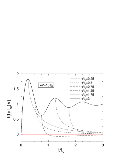
FIG. 2.: The current $I(t)$ in response to a pulsed bias potential of magnitude $eV=10\Gamma_{a}$, for different pulse durations $\tau$. Here $k_{B}T=0.1\Gamma_{a}$ and $t_{v}=2\pi\hbar/eV$. $I_{dc}(V)$ is the steady-state current for an $eV$ dc voltage bias. The asymptotic fall-off current oscillates with $\sin(2\pi\tau/t_{v})$, resulting in the reversal of the current for $\tau/t_{v}=3/4$.

Although our solution clearly captures the essential findings of the non-crossing approximation, there are two major omissions to be noted. First, working with a Kondo impurity rather than an Anderson impurity, our model lacks the short charge-fluctuation time scale ($t_{0}=\hbar/\Gamma_{\rm dot}$ in the notations of Ref. [13]), which governs the very early response of a quantum dot to the abrupt change in the applied voltage bias. Second, for $0<t\leq\tau$, our solution does not show the expected decrease in saturation time for large voltage bias. [13] This decrease, which stems from the dissipative lifetime induced by the bias potential, [14] is not captured by the solvable point. On the other hand, our solution gives a very transparent picture for the role of a temperature. As the temperature is increased, $t_{d}$ crosses over from $\hbar/\Gamma_{a}$ to $\hbar/\pi k_{B}T$, which remains the only relevant time scale for $k_{B}T\gg eV$. Thus, all response times for the current are determined by the temperature in this limit.

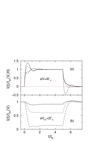
FIG. 3.: The time-dependent current for (a) a dc magnetic field $H$ and a rectangular pulsed bias potential of magnitude $eV=4\Gamma_{a}$; and (b) a dc bias potential $eV=2\Gamma_{a}$ and a rectangular pulsed magnetic field of magnitude $H$. Upper panel: Solid, dashed, dotted, and long-dashed lines correspond to $\mu_{B}g_{i}H/\Gamma_{a}=0,1,2$, and $4$, respectively. Lower panel: Solid, dotted, and long-dashed lines correspond to $\mu_{B}g_{i}H/\Gamma_{a}=1,2$, and $4$, respectively. In both cases, the pulse duration is $\tau=5t_{k}$ ($t_{k}=\hbar/\Gamma_{a}$), and the temperature is equal to $k_{B}T/\Gamma_{a}=0.1$. $I_{dc}(V,H)$ marks the steady-state current for a dc voltage bias of $eV$ and a dc magnetic field $H$.

An important advantage of the solvable point with $\Gamma_{a}=\Gamma_{b}$ is the ability to incorporate an arbitrary time-dependent magnetic field. Specifically, we find that the current $I(t)$ for a general voltage bias $eV(t)$ and an arbitrary field $H(t)$ is equal to $\frac{1}{2}\left[I_{+}(t)+I_{-}(t)\right]$, where $I_{\pm}(t)$ is the current for a zero magnetic field and an effective bias potential $eV_{\pm}(t)=eV(t)\pm\mu_{B}g_{j}H(t)$. The latter bias has a simple physical interpretation. When an electron tunnels by flipping the impurity spin, the effective potential barrier it sees is equal to $eV_{\pm}(t)$, depending on the initial impurity state, and the direction of tunneling.

Using the above decomposition of $I(t)$ into $I_{\pm}(t)$, we have computed the current for the two opposite cases of (i) a dc magnetic field $H$ and a rectangular pulsed bias potential of magnitude $eV$, and (ii) a dc bias potential of $eV$ and a rectangular pulsed magnetic field of magnitude $H$. In both cases, the pulse duration was taken to be $\tau$, with the corresponding field being equal to zero for $t<0$ and $t>\tau$. The calculation of $I_{\pm}(t)$ in each of these cases requires the generalization of Eqs. (11)–(12) to a pulsed bias potential of the form $V(t)=V_{2}$ for $0\leq t\leq\tau$ and $V(t)=V_{1}\neq 0$ otherwise, which gives

$$I_{1}(t)= I_{dc}(V_{2})-{\rm Im}\left\{e^{-ieV_{2}t/\hbar}{\cal J}(t;V_{1},V_{2})\right\},$$ (16)

$$I_{2}(t)= I_{dc}(V_{1})+{\rm Im}\left\{e^{-ieV_{1}(t-\tau)/\hbar}{\cal J}(t\!-\!\tau;V_{1},V_{2})\right\}$$ (18)

$$-{\rm Im}\left\{e^{-ieV_{2}\tau/\hbar}e^{-ieV_{1}(t-\tau)/\hbar}{\cal J}(t;V_{1},V_{2})\right\}.$$

For $t\leq 0$, the corresponding current is obviously $I_{dc}(V_{1})$.

The resulting $I(t)$ curves are depicted in Fig. 3. As is clearly seen, the combination of a bias and a magnetic field produces nontrivial interference patterns with several underlying time scales. These include $t_{d}$, $t_{\pm}=2\pi\hbar/|eV\pm\mu_{B}g_{i}H|$, and either $t_{h}=2\pi\hbar/\mu_{B}g_{i}H$ or $t_{v}$, depending on whether one is dealing with a pulsed bias potential or a pulsed magnetic field. In particular, for a pulsed bias potential and moderately large dc magnetic fields, there are current oscillations in the fall-off current, with a characteristic frequency of $\omega=\mu_{B}g_{i}H/\hbar$. Such effects should be observable in ultra small quantum dots.

REFERENCES

- [1] D. Goldhaber-Gordon et al., Nature 391, 156 (1998); D. Goldhaber-Gordon et al., Phys. Rev. Lett. 81, 5225 (1998).
- [2] S. M. Cronenwett et al., Science 281, 540 (1998).
- [3] J. Schmid et al., Physica B 258, 182 (1998).
- [4] F. Simmel et al., Phys. Rev. Lett. 83, 804 (1999).
- [5] P. W. Anderson, Phys. Rev. 124, 41 (1961).
- [6] U. Gerland et al., Phys. Rev. Lett. 84, 3710 (2000).
- [7] J. Appelbaum, Phys. Rev. Lett. 17, 91 (1966); P. W. Anderson, Phys. Rev. Lett. 17, 95 (1966).
- [8] L. I. Glazman and M. E. Raikh, Pis’ma Zh. Eksp. Teor. Fiz. 47, 378 (1988) [JETP Lett. 47, 453 (1988)]; T. K. Ng and P. A. Lee, Phys. Rev. Lett. 61, 1768 (1988); S. Hershfield, J. H. Davies, and J. W. Wilkins, Phys. Rev. Lett. 67, 3720 (1991); Y. Meir, N. S. Wingreen, and P. A. Lee, Phys. Rev. Lett. 70, 2601 (1993).
- [9] A. Schiller and S. Hershfield, Phys. Rev. B 51, 12896 (1995); A. Schiller and S. Hershfield, ibid. 58, 14978 (1998).
- [10] M. H. Hettler and H. Schoeller, Phys. Rev. Lett. 74, 4907 (1995); T. K. Ng, Phys. Rev. Lett. 76, 487 (1996); Y. Goldin and Y. Avishai, Phys. Rev. Lett. 81, 5394 (1998); A. Kaminski et al., Phys. Rev. Lett. 83, 384 (1999).
- [11] A. Schiller and S. Hershfield, Phys. Rev. Lett. 77, 1821 (1996).
- [12] For a first application of ac fields to a quantum dot in the Kondo regime, see J. M. Elzerman et al., J. Low Temp. Phys. 118, 375 (2000).
- [13] M. Plihal, D. C. Langreth, and P. Nordlander, Phys. Rev. B 61, 13341 (2000).
- [14] N. S. Wingreen and Y. Meir, Phys. Rev. B 49, 11040 (1994).
- [15] G. Toulouse, Phys. Rev. B 2, 270 (1970).
- [16] V. J. Emery and S. Kivelson, Phys. Rev. B 46, 10812 (1992).
- [17] The Toulouse limit was also applied to a different type of nonequilibrium dynamics, i.e., that of a dissipative multiwell system. See U. Weiss and M. Wollensak, Phys. Rev. B 37, 2729 (1988); U. Weiss et al., Z. Phys. B 84, 471 (1991).