Domain Coarsening in Electroconvection

Abstract

We report on experimental measurements of the growth of regular domains evolving from an irregular pattern in electroconvection. The late-time growth of the domains is consistent with the size of the domains scaling as $t^{n}$. We use two isotropic measurements of the domain size: the structure factor and the domain wall length. Measurements using the structure factor are consistent with $t^{1/5}$ growth. Measurements using the domain wall length are consistent with $t^{1/4}$ growth. One source of this discrepancy is the fact that the distribution of local wavenumbers is approximately independent of the domain size. In addition, we measure the anisotropy of the growing domains.

There are many situations where a system experiences a rapid change of an external parameter, or quench, such that the state of the system after the quench is not an equilibrium or steady-state phase. Domains of the new equilibrium phase form, and the subsequent growth of these domains, or coarsening, is often characterized by a single scale size for the domains that follows a power-law growth. There has been a great deal of both theoretical and experimental study of this process for systems where both the initial state prior to the quench and final state after the quench are thermodynamic equilibrium states at finite temperature [1]. We are interested in the analogous process for systems that are driven out of equilibrium. For such systems, neither the initial nor the final state is in thermodynamic equilibrium; however, they are steady-states of the system. The first situation will be referred to as a thermodynamic system and the second situation as a driven system. For driven systems, studies of model equations suggest power-law scaling of the late-time domain growth; however, the value of the growth exponent depends on the measurement scheme [2, 3, 4]. Experimentally, the coarsening of random patterns after a ramp in the control pattern has been studied, but growth exponents for domain size were not measured [5]. Thermodynamic systems with stripes have been studied experimentally using block copolymers [6].

In spatially extended systems that are driven out of equilibrium, there is generally a transition from a uniform state to a periodic, or “stripe”, state at a critical value $R_{c}$ of the external control parameter $R$ [7]. A quench corresponds to a rapid change of $R$. For values reasonably close to $R_{c}$, these systems are often well described by model equations that are similar to, and in some cases identical to, the equations used to study coarsening in thermodynamic systems [7]. However, in a driven system, there is generally no equivalent of a free-energy that governs the growth of the domains, and the periodic structure complicates the dynamics. Therefore, the question of how the ordering proceeds in driven systems, and the differences and similarities with thermodynamic systems, is one of great interest.

Simulations of potential [3, 4] and nonpotential [3] forms of the Swift-Hohenberg equation have been used to study quenches in driven systems [2, 3, 4]. In both cases, characterization of the growth by the structure function $S(k)$ suggests a length scale that grows as $t^{1/5}$ [3, 4]. In contrast, the growth exponent determined from the orientational correlation function is consistent with $1/4$ [3, 4] for potential dynamics and with $1/2$ [3] for nonpotential dynamics. There is no explanation of the discrepancy between the $S(k)$ and orientational correlation function measurements; however, the length scales determined by these measures do not have the same immediate interpretation [4]. The orientational correlation function results agree with experiments in block copolymers [6].

We have made experimental measurements of coarsening in an anisotropic, driven system: electroconvection in a nematic liquid crystal [8]. A nematic liquid crystal is a fluid in which the molecules align on average along a particular axis, referred to as the director [9], which we take as the x-axis. Because the system is anisotropic, there are only two possible orientations of the domains. This is fundamentally different than previous simulations and experiments. One expects a different scale size parallel and perpendicular to the preferred direction in the system. Our measurement of these scale sizes show that not only are the magnitudes of the length scales different, but they also coarsen with different growth exponents. We also measure isotropic properties of the domain growth and find that they are in surprising agreement with the predictions of the Swift-Hohenberg simulations [3, 4]. Finally, our measurements show that the domain size and wavenumber variation have different growth exponents, which explains the discrepancy between the $S(k)$ and orientational correlation function measurements.

For electroconvection, the liquid crystal is placed between two glass plates with the director aligned parallel to the plates and along a single axis. The liquid crystal is doped with ionic impurities. An ac voltage is applied perpendicular to the plates. Above a critical value of the applied voltage $V_{c}$, there is a transition to a state that consists of convection rolls with a corresponding periodic variation of the director and charge density. We studied oblique rolls, i.e. patterns that have a nonzero angle $\theta$ between the wavevector and the alignment of the undistorted director. Oblique rolls with the same wavenumber $k$ but at $\theta$ (zig rolls) and $-\theta$ (zag rolls) are degenerate. The initial transition in this system is to a pattern that consists of the superposition of four modes: right- and left-traveling zig and zag rolls. The interaction of these four modes leads to irregular spatial and temporal variations of the amplitudes of each of the modes [10], i.e. spatiotemporal chaos [7, 11]. For traveling rolls, a sufficiently large modulation of the amplitude of the applied voltage at twice the intrinsic frequency of the pattern stabilizes standing rolls [12, 13, 14]. For our system, either standing zig or standing zag rolls are stabilized, and the stabilized pattern exhibits regular temporal dynamics [15]. In our experiments, a quench corresponded to a rapid change of the modulation amplitude at a fixed value of $V_{rms}$. As standing waves can be stabilized both below and above $V_{c}$, two types of quenches are possible. Below $V_{c}$, the dynamics of the standing waves are potential [16], and above $V_{c}$, they are nonpotential [17]. Therefore, based on the results of Ref. [3], we expected two different growth exponents. Also, below $V_{c}$, domains of standing zig and zag rolls must first form before the system coarsens, as the initial state is spatially uniform. This process is illustrated in Fig. 1(a) - (d). Above $V_{c}$, domains of zig and zag rolls are already present after the quench, and the coarsening proceeds from this initial distribution. This process is illustrated in Fig. 1(e) - (h).

The details of the experimental apparatus are described in Ref. [15]. Commercial cells [18] with a thickness of 23 $\mu$m and 1 cm² electrodes were used. The sample temperature was maintened at $50.0\pm 0.002\ {\rm{}^{\circ}C}$. The patterns were observed from above using a modified shadowgraph setup [19] that effectively eliminated the well-known nonlinear effects in the shadowgraph image [20]. An ac voltage, $V(t)=[V_{o}+V_{m}\sin(\omega_{m}t)]\sin(\omega_{d}t)$, was applied across the sample, with $\omega_{d}/2\pi=25\ {\rm Hz}$. There are two relevant dimensionless control parameters: $\epsilon=(V_{o}/V_{c})^{2}-1$ and $b=V_{m}/V_{c}$. Here $V_{c}$ is the critical voltage for the onset of a pattern when $V_{m}=0$. There was a small, linear drift in $V_{c}$; therefore, before and after each quench, $V_{c}$ and $\omega_{h}$ were determined. Typical values were $V_{c}=15\ {\rm V_{rms}}$ and $\omega_{h}/2\pi=0.5\ {\rm Hz}$.

The system was equilibrated at $b=0$ and either $\epsilon=-0.03$ or $\epsilon=0.03$ for five minutes. For $\epsilon=-0.03$ ($\epsilon=0.03$), the transition to standing waves occurs at $b=0.03$ ($b=0.013$) [15]. For $\epsilon=-0.03$, we used a jump from $b=0$ to $b=0.05$, and for $\epsilon=0.03$, we used a jump from $b=0$ to $b=0.04$. In both cases, $\omega_{m}=2\omega_{h}$, where $\omega_{h}$ is the frequency of the pattern at onset, the Hopf frequency. A third quench was done at $\epsilon=0.03$ with $\omega_{m}=2.1\omega_{h}$. Immediately after a jump in $b$, a series of 128 images was obtained. An image was taken every $5^{th}$ cycle of the modulation, or roughly once every 5 seconds, triggered by the applied voltage to occur at $T/4$, where $T$ is the period of the modulation. In order to resolve the individual rolls, a 1.35 mm by 1.35 mm section of the sample was imaged. At the end of a typical time series, the domain size was on the order of our observation window; however, given the size of the entire sample, we were not limited by finite size effects. Unless otherwise noted, time is scaled by the director relaxation time, which for our system is 0.2 s. For $\epsilon=0.03$, we performed 20 quenches, and for $\epsilon=-0.03$, we performed 18 quenches. The domain wall length, $S(k)$, the local wavenumber distribution, $\Delta q_{x}$, and $\Delta q_{y}$ were computed for each image in the time series for a given quench. ($\Delta q_{x}$ and $\Delta q_{y}$ are defined below.) The values at each time step were averaged over all the quenches for a given $\epsilon$. These averaged values were used to compute the growth exponents, which did not change significantly after averaging 10 quenches.

If a single scale length is sufficient to describe the domain growth, both the total domain wall length and the width of the power spectrum would exhibit the same growth exponent. Because, the structure factor contains information about the range of local wavenumbers within a domain, we measured the local wavenumber using the method described in Ref. [21]. Briefly, this method involves calculating the x-component of $k$ from $|k_{x}|^{2}=-[\partial_{x}^{2}u({\bf x})]/u({\bf x})$, with a similar calculation for the y-component. Here $u({\bf x})$ is the image of the pattern. We used the central 0.82 mm by 0.82 mm region of the image in the determination of the spread $\Delta k$ of the magnitude $k$ of the local wavevector ${\bf k}$. We defined $\Delta k$ as the square root of the second moment of the distribution of $k$ about $k_{ave}$.

To determine the normalized domain-wall length $L$, the local orientation was determined from the sign of $[\partial_{xy}u({\bf x})]/u({\bf x})$. Regions with a negative (positive) value of this ratio corresponded to zig (zag) rolls and were assigned a grayscale of 0 (255). The resulting image was smoothed, producing an image in which domain walls had a value close to 128. Applying a threshold produced images in which zig regions had a value of 0, domain walls a value of 128, and zag rolls a value of 255. The domain wall “length” was taken as the total number of pixels of value 128 normalized by the total number of pixels in the image. Images from a typical sequence, after processing, are shown in Fig. 1. The processed images were also used to study the anisotropy of the growth. Since the wavelength has been factored out of the processed images, the width of the central peak in the power spectrum $S({\bf q})$ of one of these images corresponds to the length scale of the domains. Defining $\Delta q_{x}$ ($\Delta q_{y}$) as the second moment of $q_{x}$ ($q_{y}$) about ${\bf q}=0$ of $S({\bf q})$, with $q_{x}$ and $q_{y}$ the x- and y-components of ${\bf q}$, provides a measure of the inverse of the correlation length in the x and y directions.

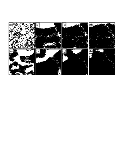
FIG. 1.: Processed images illustrating the domain growth for a quench at $\epsilon=-0.03$ (images (a) - (d)) and for a quench at $\epsilon=0.03$ (images (e) - (h)). The images cover an area of 1.35 mm by 1.35 mm, and the processing method is described in detail in the text. The black regions are areas of zig rolls, and the white areas are regions of zag rolls. Image (a)/(f) was taken 5 s after the quench, and the subsequent images are all 160 s apart.

The measurements based on $S(k)$ used the same method as described in Ref. [3]. The structure factor (the square of the Fourier transform) was averaged over all angles. The relevant peak in the resulting $S(k)$ was fit to a Lorentzian squared, and the width $\delta k$ was defined as the half width at half height. This method is an isotropic measure of the domain growth and is used to ensure that our results are directly comparable to Ref [3].

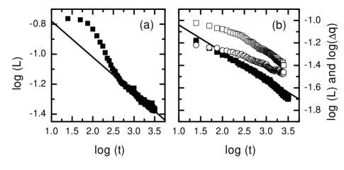
FIG. 2.: This shows a plot of $\log(L)$ versus $\log(t)$. Here $L$ is the total length of the domain wall in the region of study. Plot (a) is for the quench at $\epsilon=-0.03$, and plot (b) is for the quench at $\epsilon=0.03$. The solid lines are linear fits to the data. The line in (a) has a slope of $-0.240\pm 0.004$, and the line in (b) has a slope of $-0.243\pm 0.003$. In (b), the open symbols are the results for $\Delta q_{x}$ (circles) and $\Delta q_{y}$ (squares).

Figures 2a and 2b show the results for the domain wall length $L$ for the $\epsilon=-0.03$ and $\epsilon=0.03$ quenches, respectively. Here $\log(L)$ is plotted versus $\log(t)$. For the quench at $\epsilon=0.03$, the behavior is consistent with power law scaling essentially immediately after the quench. For $\epsilon=-0.03$, the system is not consistent with power law scaling until $\log(t)\approx 2.5$. This difference is reasonable given that the domains must first form for the quench at $\epsilon=-0.03$. Also, the scaling occurs in both systems at roughly the same scale size for the domains, $\log(L)\approx-1.2$. The decay of the domain-wall length is consistent with scaling as $t^{-1/4}$. The solid line in Fig. 2a is a fit over the range $2.5<\log(t)<3.5$ and has a slope of $-0.24$. The solid line in Fig. 2b is a fit over the range $2.0<\log(t)<3.2$ and also has a slope of $-0.24$.

Figure 2b also shows the results for $\Delta q_{x}$ (open circles) and $\Delta q_{y}$ (open squares). As is suggested by the images in Fig. 1, the domains tend to be larger along the director (x-direction). This is confirmed by the relative magnitudes of $\Delta q_{x}$ and $\Delta q_{y}$. Also, the two lengths coarsen with different exponents, where the growth exponent perpendicular to the director is consistent with the exponent measured using the domain-wall length. A similar result holds for the $\epsilon=-0.03$ quench, with the same delay in the onset of scaling as seen in the wall length.

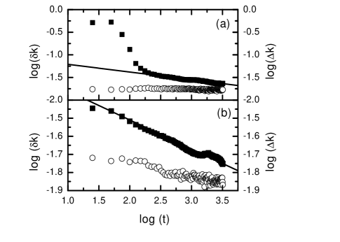
FIG. 3.: This shows a plot of $\log(\delta k)$ versus $\log(t)$ using the left hand axis and solid symbols, and a plot of $\log(\Delta k)$ versus $\log(t)$ using the right hand axis and open symbols. Plot (a) is for the quench at $\epsilon=-0.03$, and plot (b) is for the quench at $\epsilon=0.03$. The solid lines are linear fits to the solid data. The line in (a) has a slope of $-0.170\pm 0.003$, and the line in (b) has a slope of $-0.165\pm 0.002$.

Figures 3a and 3b show $\log(\delta k)$ and $\log(\Delta k)$ versus $\log(t)$ for the quenches at $\epsilon=-0.03$ and $\epsilon=0.03$, respectively. The behavior is consistent with power-law scaling almost immediately for $\epsilon=0.03$ and at later times for $\epsilon=-0.03$. The scaling sets in for both quenches at approximately the same domain size. For both quenches, the scaling of $\delta k(t)$ is consistent with $t^{-1/5}$ decay, as found in simulations [3, 4]. For $\epsilon=-0.03$, the solid line is a fit over the region $2.5<\log(t)<3.5$ and has a slope of -0.17. For $\epsilon=0.03$, the solid line is a fit over the region $2.0<\log(t)<3.2$ and has a slope of -0.16. However, for both cases, the variation in the local wavenumber $\Delta k$ is a significant fraction of $\delta k$ in the possible scaling regime and is roughly constant in time. Therefore, $\delta k$ is not an accurate measure of the growth of the domain size, but a complicated convolution of the domain size and $\Delta k$. Accounting for this effect, measurements of the coarsening parallel and perpendicular to the director based on individual peaks of $S({\bf k})$ are consistent with the anisotropy determined from $S({\bf q})$ of the processed images.

Despite the different symmetries, the isotropic measures of the domain growth in electroconvection agree well with the simulations of the Swift-Hohenberg model [2, 3, 4] and experiments in block copolymers [6]. Understanding this agreement will require further work. In particular, the work with block copolymers attributes the exponent of $1/4$ to the dynamics of topological defects [6]. Because of the anisotropy, the relevant defect dynamics in electroconvection are different. For example, there are no regions where the roll orientation changes continuously, only sharp domain walls.

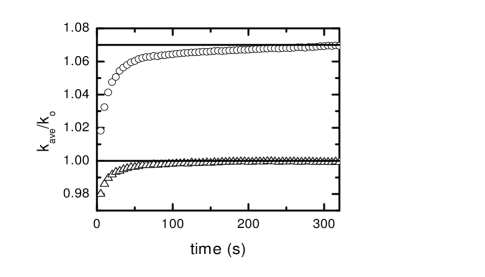
FIG. 4.: This shows a plot of $k_{ave}/k_{o}$ versus time. The triangles are for the quench at $\epsilon=0.03$ with $\omega_{m}=2.0\omega_{h}$, and the circles are for the quench at $\epsilon=0.03$ with $\omega_{m}=2.1\omega_{h}$. The lines are a guide to the eye.

One discrepancy is our observation of a growth exponent of $1/4$ for both $\epsilon<0$ and $\epsilon>0$. For $\epsilon>0$, we expected an exponent of $1/2$ [3]. One possible explanation of the discrepancy is the potential existence of long-time transients. An analysis of the Swift-Hohenberg equation for patterns with $k=k_{o}$ suggests a long-time transient regime for which the growth exponent is $1/4$ [2, 4]. In our system, the dispersion relation fixes the average wavenumber $k_{ave}=k_{o}$ for $\omega_{m}=2\omega_{h}$. To vary $k_{ave}$, we performed a quench at $\omega_{m}=2.1\omega_{h}$, for which $k_{ave}=1.07k_{o}$. The quench was at $\epsilon=0.03$ to a value of $b=0.04$. Measurements of $L$ were consistent with a growth exponent of $1/4$. However, the average wavenumber exhibited a slow approach to a steady state (see Fig. 4), suggesting that this growth exponent also corresponds to a transient regime. Because there is no significant evolution of the wavenumber spread, we plan to study larger regions of the sample, without resolving the individual rolls, for longer times by exploiting optical properties of the patterns. This will allow for the possibility of observing a crossover to a different growth exponent.

The authors acknowledge funding from NSF grant DMR-9975479. L. Purvis was supported by NSF Research Experience for Undergraduates grant PHY-9988066. M. Dennin would like to thank Michael Cross and Herman Riecke for useful discussions.

REFERENCES

- [1] A. J. Bray, Advances in Physics 43, 357 (1994).
- [2] K. R. Elder, J. Vinals, and M. Grant, Phys. Rev. Lett. 68, 3024 (1992).
- [3] M. C. Cross and D. I. Meiron, Phys. Rev. Lett. 75, 2152 (1995).
- [4] J. J. Christensen and A. J. Bray, Phys. Rev. E 58, 5364 (1998).
- [5] C. W. Meyer, G. Ahlers, D. S. Cannell, Phys. Rev. A 44, 2514 (1991).
- [6] C. Harrison, D. H. Adamson, Z. Cheng, J. Sebastian, S. Sethuraman, D. Huse, R. A. Register, and P. M. Chaikin, Science 290, 1558 (2000).
- [7] For reviews of pattern formation, see M. C. Cross and P. C. Hohenberg, Rev. Mod. Phys. 65, 851 (1993), and J. P. Gollub and J. S. Langer, Rev. Mod. Phys. 71, s396 (1999).
- [8] Review articles on electroconvection can be found in I. Rehberg, B. L. Winkler, M. de la Torre Juárez, S. Rasenat, and W. Schöpf, Festkörperprobleme 29, 35 (1989); S. Kai and W. Zimmermann, Prog. Theor. Phys. Suppl. 99, 458 (1989); and L. Kramer and W. Pesch, Annu. Rev. Fluid Mec. 27, 515 (1995).
- [9] P. G. de Gennes, The Physics of Liquid Crystals (Claredon Press, Oxford, 1974); S. Chandrasekhar, Liquid Crystals (Cambridge University Press, Cambridge, England, 1992).
- [10] M. Dennin, G. Ahlers, and D. S. Cannell, Science 272, 388 (1996).
- [11] For a recent review of experimental examples of spatiotemporal chaos, see G. Ahlers, Physica A 249, 18 (1998).
- [12] H. Riecke, J. D. Crawford, and E. Knobloch, Phys. Rev. Lett. 61, 1942 (1988).
- [13] D. Walgraef, Europhys. Lett. 7, 485 (1988).
- [14] I. Rehberg, S. Rasenat, J. Fineberg, M. de la Torre Juáurez, and V. Steinberg, Phys. Rev. Lett. 61, 2449 (1988).
- [15] M. Dennin, Phys. Rev. E, (2000).
- [16] H. Riecke, Europhys. Lett. 11, 213 (1990).
- [17] H. Riecke, private communication.
- [18] E.H.C. CO., Ltd., 1164 Hino, Hino-shi, Tokyo, Japan.
- [19] H. Amm, R. Stannarius, and A. G. Rossberg, Physica D 126, 171 (1999).
- [20] S. Rasenat, G. Hartung, B. L. Winkler, and I. Rehberg, Experiments in Fluids 7, 412 (1989).
- [21] D. A. Egolf, I. V. Melnikov, and E. Bodenschatz, Phys. Rev. Lett. 80, 3228 (1998).