Phase Fluctuations and
Pseudogap Phenomena
Abstract
This article reviews the current status of precursor superconducting phase fluctuations as a possible mechanism for pseudogap formation in high-temperature superconductors. In particular we compare this approach which relies on the two-dimensional nature of the superconductivity to the often used -matrix approach. Starting from simple pairing Hamiltonians we present a broad pedagogical introduction to the BCS-Bose crossover problem. The finite temperature extension of these models naturally leads to a discussion of the Berezinskii-Kosterlitz-Thouless superconducting transition and the related phase diagram including the effects of quantum phase fluctuations and impurities. We stress the differences between simple Bose-BCS crossover theories and the current approach where one can have a large pseudogap region even at high carrier density where the Fermi surface is well-defined. The Green’s function and its associated spectral function, which explicitly show non-Fermi liquid behaviour, is constructed in the presence of vortices. Finally different mechanisms including quasi-particle-vortex and vortex-vortex interactions for the filling of the gap above are considered.
keywords:
high-temperature superconductivity, pseudogap, phase fluctuationsPACS: 74.25.-q — General properties; correlation between physical properties in normal and superconducting states; 74.40.+k — Fluctuations; 74.62.Dh — Effects of crystal defects, doping and substitution; 74.72.-h — High- compounds
, ,
Present address: Institut de Physique, Université de Neuchâtel, CH-2000, Neuchâtel, Switzerland
1 Introduction
1.1 Pseudogap Phenomena in High- superconductors
The discovery of high temperature superconductors (HTSC) [1] revealed new problems in solid state physics in general and in the theory of superconductivity in particular. A combination of factors, including unusual magnetic and electronic properties, a lowered dimensionality, closeness to the metal-insulator transition and relatively low carrier densities, makes the construction of an appropriate theory both difficult and far from resolved. There is no consensus as to the correct theoretical approach. It is even unclear as to which physical features of cuprate superconductors should be considered as the basis for the correct theory.
One of the clearest differences between the BCS scenario of superconductivity and superconductivity in the cuprates is the existence of a pseudogap. This is simply a depletion of the single particle spectral weight around the Fermi level [2, 3] (see also a recent excellent experimental review by Timusk and Statt [4]).111Note that the word “pseudogap” for HTSC was originally suggested by Friedel [5], although in a different context. The notion of pseudogap has been used before in other areas such as 1D conductors. The earliest experiments to reveal gap-like behaviour in the normal state were the NMR measurements of the Knight shift (see Refs. in [4]) which probes the uniform spin susceptibility.

Based on the NMR data the phase diagram presented in Fig. 1 was suggested for the cuprate superconductors.
In Fig. 1 there are two main phase boundaries. The first is the transition into a long-range antiferromagnetic state at the Néel ordering temperature, , in the very low doping regime. The second is the transition into a superconducting state, with the maximal critical temperature at approximately holes/CuO2 unit cell. With respect to the maximal , under-, optimally and overdoped regimes are distinguished.
In addition to the above-mentioned phase boundaries, two crossover lines, and , are evident in these materials, even at rather low doping levels. It must be noted, however, that the experimental determination of these lines is still somewhat controversial. We will return to the discussion of how the different theoretical approaches treat the phase diagram.
At the upper crossover temperature the Knight shift changes behaviour. Above it is temperature independent, while below it decreases linearly with temperature. Below the lower crossover temperature the Knight shift decreases supra-linearly with temperature. It was suggested (see [4]) that these two crossover temperatures may originate from two different physical phenomena. In particular the lower crossover temperature appears to be the result of a gap appearing in the spectrum of elementary antiferromagnetic excitations. This manifestation of the pseudogap phenomenon was thus called a spin gap.
Subsequently the optical conductivity data (which has been discussed in detail in the review [6]) showed in addition a gapping of the charge degrees of freedom. Specific heat data (see Refs. in [4]) also provided evidence that an electronic gap opens below . Considerable recent experimental progress in angle resolved photo-emission spectroscopy (ARPES) (see for example the reviews [7, 8]) gives an experimental window on the single-particle spectral function and other fundamental quantities such as the electron self-energy [9]. In these experiments one can clearly see the presence of a strong reduction in the quasi-particle weight, or equivalently a pseudogap, below . Until recently most ARPES measurements were performed for the photon energy range between 19 and 25. The most recent data [10], which was taken with a higher photon energy of 33, is in contradiction with the previous data. This question is now under intensive investigation [11], particularly since ohmic losses may alter the ARPES spectra [12].
An explanation of the pseudogap phenomenon is regarded as one of the most important unresolved questions in the theory of superconductivity. The ARPES and the scanning tunnelling spectroscopy (STS) experiments (see Refs. in [4]) showed a smooth crossover from the pseudo- to superconducting gap, so that in these single-particle spectroscopies, the transition into the true superconducting state at is barely noticeable. Moreover the pseudo- and superconducting gaps also reveal experimentally the same -wave symmetry of the order parameter [13, 14] (see also the reviews [15, 4, 8]). We note, however, that at this stage the question of the symmetry of the order parameter in HTSC is still under discussion [16]. For example, it is shown in [17, 18, 19] that the observed symmetry of the order parameter cannot be fitted by only the lowest harmonic of the -wave order parameter. Furthermore, a recent experiment with twisted Josephson junctions in the Bi-cuprates [20], is in favour of an extended -wave order parameter, and has shown the absence of a -wave part in the order parameter. It has also been suggested that a transition from the symmetry to the symmetry could be induced by an external magnetic field [21] and may be observed in the cuprates. Despite remaining uncertainties in the experimental data, the existence of a pseudogap and a corresponding crossover temperature is well established, and the underlying physics demands an explanation.
1.2 Current theoretical explanations for the origin of the pseudogap: magnetic, spin-density waves, stripes, etc.
Due to the extremely complex structural and electronic nature of the cuprate systems [22], and the somewhat controversial nature of much of the current experimental data, there are many theoretical attempts to explain pseudogap behaviour.

As an example, we show two theoretical phase diagrams [23]. The first is based on the theory developed by Pines and collaborators of the nearly antiferromagnetic Fermi liquid [24] (Fig. 2-A). The second is based on the arguments of Emery and Kivelson (Fig. 2-B) which are based on superconducting phase fluctuations [25, 26] (see also [27]). Both these theories are attempting to interpret the experimental phase diagram presented in Fig. 1, and give in addition, predictions about the less well experimentally studied regions of the diagram. As an example, the continuation of the pseudogap lines below on Fig. 2 should be interpreted [23] as “what would be present if there was no superconducting phase”. This can be realized in practice by applying a magnetic field.
At this stage most interpretations of the NMR experiments [28, 29] support the magnetic theory of the pseudogap (or to be more exact the existence of a spin gap). On the other hand the ARPES [4, 8, 30] and STS [4, 31, 32] experiments can and have been interpreted using theories based solely on precursor superconducting fluctuations (see Sec. 1.3). This claim however depends on the precise way in which the experimental results have been interpreted, and how well developed the particular theory is for the given range of doping and/or the applied magnetic field if present. For instance, it is argued in [23] that the current NMR data still do not exclude the scenario based on the superconducting fluctuations and that more measurements in the overdoped cuprates are needed. An opposite point of view which supports the diagram in Fig. 2-A is presented in a very recent survey of the experimental data [33]. However, so evident disagreement between [33] and [23] (see also [3]) once more demonstrates vividly that there is no consensus about the true shape of the cuprate phase diagram.
Another possible explanation relates the pseudogap to charge- and/or spin-density waves [16] (see also very recent paper [34] and Refs. therein). A theory based on the phase separation in the form of a strip structure of metallic and insulating domains with a spin gap in the AFM regions has been suggested by Emery, Kivelson and Zachar [35] (see also the more recent paper [36]). Such a separation is accompanied by the formation of a pairing amplitude through a proximity effect between non-magnetic metallic and AFM insulating stripes, but with large phase fluctuations. Below this theory has much in common with the more phenomenological approach based on the 2D attractive Hubbard model discussed here simply because both theories are based on phase fluctuations. A stripe-phase quantum-critical-point scenario for high- superconductors which has much in common with that of Ref. [35] has been developed in [37]. symmetry [38] which unifies the antiferromagnetic and superconducting behaviour has also been used to explain pseudogap behaviour. Finally spin-charge separation [39] has been invoked. This last theory also predicts [40], in a quasi-2D system, a novel spin-metal phase with a nonzero spin diffusion constant at zero temperature. It is therefore entirely conceivable that the phase diagrams shown earlier are incomplete, and that new phases await discovery and/or confirmation, particularly if one applies a magnetic field (see for example [41]).
1.3 Precursor superconducting fluctuations in particular phase fluctuations
As mentioned above, one major thrust suggests that some form of precursor superconducting fluctuations or in particular phase fluctuations [25, 26, 27] are responsible for the pseudogap phenomenon. This assumption differs in principle from, for example, bipolaron theory of high- superconductivity (see the review [42] and textbook [43]), where a very strong electron-phonon coupling is assumed and where the bose-pairs are formed as stable units at temperatures higher than the temperature of the superconducting (in this case superfluid) transition.
An incoherent pair tunnelling experiment [44] has been proposed which may be able to answer whether superconducting fluctuations are truly responsible for the pseudogap behaviour or whether another mechanism is involved. A second test of the nature of the condensation which comprises comparing two methods of determination of the gap has been proposed in [45]. The first method for finding the gap is related to the single-particle excitation energy , measured by ARPES or STS. The second method is related to the energy coherence range , defined by Andreev reflection. Finally, Andreev interferometry — the sensitivity of the tunneling current to spatial variations in the local superconducting order at an interface — has also been proposed recently [46] as a probe of the spatial structure of the phase correlations in the pseudogap state.
One cannot however exclude the possibility that the pseudogap is the result of a combination of various factors, e.g. spin and superconducting (including phase) fluctuations222Indeed, the anisotropy of the spin subsystem in HTSC belongs to an easy-plane type which in turn implies that the magnetic vectors (averaged spins) can be described by a model similar to the model. The loss of long-range magnetic order under doping and the appearance of magnetic correlation length (see [22]) results in some sense in the formation of a gap in the spin spectrum. Superconducting phase fluctuations, as will be seen in Sec. 5, can also be described by a -model and their phase transition behaviour is similar. (see, for example, models [47, 48] where the interplay of antiferromagnetic and -wave pairing fluctuations has been recently studied).
Different authors argue that different types of superconducting fluctuations are responsible for the pseudogap. The simplest example of a theory which has the pseudogap/gap in the normal state is the so-called BCS-Bose crossover theory.
Imagine starting from the weak coupling limit, which is well described by BCS theory [49], and gradually increasing the intensity of the attraction between the electrons. If the coupling is sufficiently strong, one no longer needs the presence of the Fermi surface which was essential in the BCS limit for the formation of Cooper pairs in metals [50]. The size of the Cooper pairs decreases until they can be regarded as almost structureless singlet bose-particles. The temperature of formation of these particles is given by the BCS pairing temperature, which is determined by the strength of the coupling. However in contrast to the BCS case, these “pre-formed” bosons condense into a single superfluid quantum state not at , but only at the temperature of Bose-Einstein condensation (BEC), . It is obvious that even above one will need to add extra energy to break up these pairs and this should lead to the gap-like features observed above . This argument is strictly valid only in 3D. Note that in the space of lowered (2D or 1D) dimensionality the formation of local pairs does not demand as strong an attraction as in 3D and the condensation process (see below) is not BEC.
There is even some evidence [51, 52] from time-resolved optical spectroscopy measurements of the quasi-particle relaxation dynamics that pre-formed pairs do exist in the underdoped YBa2Cu3O7-δ. We shall describe the history of the BCS-Bose crossover problem in Sec. 2 and consider a number of simple 2D models in Sec. 3 in the review since this problem appears to be very useful for a better understanding of superconducting fluctuations in general. Furthermore we believe that the BCS-Bose crossover problem is in its own right an exciting chapter in the history of research on superconductivity.
It is, however, rather difficult to combine the arguments about the existence of the pre-formed local pairs with the fact that the one observes a gapped Fermi surface in HTSC [4, 8]. In contrast the simple BCS-Bose crossover models (see for the reviews [53, 54]) predict its absence in precisely the Bose limit of pre-formed pairs. It follows from these observations that the attraction between carriers in HTSC is not strong enough to destroy the Fermi surface, so that the pairs above appear to be short-lived (the same is true for bipolarons [42, 43]). The presence of such resonant pairs above may still substantially affect the normal state properties of the system and this effect has been investigated in the papers of Levin et al. [55, 56, 57]. We also note that for spatially inhomogeneous systems it may be possible to have a well defined Fermi surface and yet regions of low carrier densities where pre-formed local pairs are present [58].
Up to this point our arguments were essentially independent of the dimensionality of the superconductivity. Of course as mentioned above, if one considers the 3D case, stronger attraction is necessary to reach either the Bose limit or resonant pair regime than for the 2D system. It is known, however, that all HTSC are highly anisotropic quasi-2D systems with an almost 2D character of the conducting, superconducting and magnetic properties. Indeed because the coherence length is less than a lattice spacing in the direction perpendicular to the CuO2 planes (-direction), the superconductivity in the copper oxides takes place mainly in the weakly connected interacting CuO2 layers (or their blocks). This is the reason why pure 2D models of HTSC are commonly accepted and studied. Undoubtedly the cuprate layers do exchange carriers even if these layers are situated in different unit cells (blocks). The mechanism for this transport (by coherent or incoherent (including pair) electronic tunnelling) is not yet established (see, for example, [6]).
There is no doubt nonetheless that one must take into account the possibility of different (for instance, direct or indirect) interlayer hoppings to develop the full theory of HTSC. Strictly speaking therefore, one needs to consider quasi-2D models of these superconductors. In practice, however, predominantly either 2D (or 3D) models have been considered with only a few attempts to consider quasi-2D models. This is, of course, related to the fact that the theoretical analysis even for the relatively simple attractive model is complicated. This is due to the necessity to go beyond the mean-field approximation, which proved good for BCS theory, and to take into account the well developed fluctuations of the superconducting order parameter.
It can be seen from the anisotropy of the conductivity that the influence of the third dimension varies strongly from one family of cuprates to the other. For example, this anisotropy reaches for the Bi- and Tl-based cuprates, while its value for YBaCu3O6+δ compound is close to . It seems therefore plausible that in the HTSC Bi(Tl)-compounds the transport in the -direction is incoherent, while in the Y-ones this transport is coherent at least near the optimal doping.
These brief remarks are intended to indicate how difficult it is to take into account the layered structure of HTSC. As a further example, we note that the interlayer tunnelling mechanism proposed by Anderson [59], and based on the layered structure of the cuprates, was considered as a leading candidate for the theory of HTSC superconductivity until a significant discrepancy with experiment was revealed [60].
One should also mention that the effect of interaction between the layers has been recently experimentally studied in [61] by intercalating an organic compound into bismuth-based cuprates. Even though the distance between layers increased dramatically the value of was almost unchanged from that for the pristine material. This provides unambiguous evidence that the superconductivity in layered cuprates is intrinsically of a 2D nature.
The low-dimensionality of HTSC along with a relatively small (at least in comparison to ordinary metals) carrier density provide especially good conditions for the formation of different types of vortex excitations. Although the superconducting transition at itself belongs to universality class, the large anisotropy of certain HTSC should lead to the Berezinskii-Kosterlitz-Thouless (BKT) [62] 2D XY regime over a very wide temperature range, until a crossover to 3D critical behaviour over a rather narrow temperature range (see, for example, the textbook [63]). One also expects that the transition temperature could well be practically unchanged [64], . Thus, outside the transition region the low-energy physics will be governed by the vortex fluctuations333In a strictly 2D system the BKT transition is associated with proliferation of unbound vortex-antivortex pairs. Weak coupling between the planes leads to correlated motion between vortices in adjacent planes which form 3D vortex loops close to the critical temperature. The transition to the disordered phase is then characterized by the appearance of vortex loops with arbitrarily large radii [65]., so one may expect the 2D models which we are going to discuss below to be especially relevant for the description of the pseudogap phase. Thus we arrive at the picture of Emery and Kivelson [25, 26] (see also earlier paper by Doniach and Inui [66]) where the role of the phase fluctuations of the superconducting order parameter, particularly the vortex excitations is especially important. Indeed this picture has been recently supported experimentally [67, 68] by the measurements of the screening and dissipation of a high-frequency electromagnetic field in Bi-cuprate films. These measurements provide evidence for a phase-fluctuation driven transition from the superconducting to normal state.
Without pretending to present the whole picture (this is now practically impossible), we take the point of view that the effect of low dimensionality is leading to strong order-parameter phase fluctuations, and the dependence of the conducting properties on doping, are among the key ingredients of any proposed theory. We shall use general physical assumptions and relatively simple models (which permit much analytical calculation) to discuss the new properties of HTSC, including the pseudogap, based on the assumptions given above. As we have discussed above, there is no consensus about the origin of the pseudogap. We therefore believe that all currently existing theories of pseudogap behaviour should be developed until their predictions can both be experimentally tested and contrasted with the predictions from the competing theories. Thus the main goal of this review is to outline recent developments in the theory based on phase fluctuations.
1.4 Outline
This review focuses on the simplest pairing Hamiltonians but in the limit of two dimensions and low carrier density. As such we emphasize the separation into modulus and phase variables so essential in two dimensions. Not only are these models the simplest prototype Hamiltonians in which to discuss phase fluctuations and pseudogap behaviour, but as we shall demonstrate, illustrate many of the properties of the wider class of theories based on phase fluctuations.
In Section 2 we consider a brief historical introduction to the BCS-Bose crossover as the simplest theory displaying a pseudogap. In particular we critically discuss the role of dimensionality and indicate why phase fluctuations are vital in the extreme two dimensional limit. In Section 3 we present the BCS-Bose crossover in a variety of models but at zero temperature where mean field theory still applies. In particular we focus on how the inclusion of more realistic Hamiltonians influence the crossover. The effects discussed in this section include the role of -wave pairing, the role of the retardation of the interaction, and the effect of interlayer couplings. We stress that the theory of phase fluctuations is not in fact synonymous with the BCS-Bose crossover. In Section 4 we briefly sketch the corresponding results at finite temperature obtained using the -matrix theory. These results have been derived predominantly in three dimensions and we indicate how this approach breaks down in the 2D limit. In Section 5 we present the BCS-Bose crossover in two dimensions at finite temperature. The superconducting transition temperature in this case is the Berezinskii-Kosterlitz-Thouless transition temperature. Particular attention has been paid to the important effects of quantum phase fluctuations, Coulomb repulsions and the observed presence of non-magnetic impurities. In Sections 6 and 7 we construct the single particle Green’s function and the corresponding spectral density which has been measured in recent ARPES experiments. We indicate the non-Fermi liquid behaviour induced by phase fluctuations and discuss how various mechanisms can “fill” the mean-field gap to give pseudogap behaviour. Section 8 presents our conclusions.
2 A history of the BCS-Bose crossover problem
2.1 Early history
The idea that the composite bosons (or local pairs as they are sometimes called) exist and define the superconducting properties of metals is in fact more than 10 years older than the BCS theory. As early as 1946, a sensational communication appeared saying that the chemist-experimentalist Ogg had observed superconductivity in the solution of Na in NH3 at 77K [69]. It is very interesting that the researcher made an attempt to interpret his own result in terms of the BEC of paired electrons. Unfortunately, the discovery was not confirmed and both it and his theoretical concept, were soon completely forgotten (for the details see e.g. [70, 71]).
It is instructive to note that the history of superconductivity has many similar examples. Probably, this explains why Bednorz and Müller named their first paper ”Possible high- superconductivity…” [1]. And even today there appear many unconfirmed communications about room-temperature superconducting transitions.
A new step in the development of the local pair concept, was taken in 1954 by Schafroth who in fact re-discovered the idea of the electronic quasi-molecules [72]. This idea was further developed in the Schafroth, Blatt and Butler theory of quasi-chemical equilibrium [73], where superconductivity was considered versus the BEC. Such a scenario, unfortunately, could not compete with the BCS one due to some mathematical difficulties which did not permit the authors to obtain the famous BCS results. Then the triumph of the BCS theory replaced the far more obvious concept of the local pairs and their BEC by the Cooper ones and their instability which takes place in the necessary presence of a Fermi surface (or more precisely a finite density of states at the Fermi level). In contrast for the local (i.e. separated) pairs the formation is not in principle connected to this density of electronic states. Also unlike the local pairs, the Cooper ones are highly overlapping in real space. More exactly there are no pairs in real space and the Cooper pairing should be understood as a momentum space pairing.
Later experimental results reminded physicists of the existence of local pairs. Indeed, it was Frederikse et al. [74] who found that the superconducting compound SrTiO3 (K) has a relatively low density of carriers and, moreover, this density is controlled by Zr doping. The first deep discussion of the possibility of the BCS-Bose crossover and electron binding above the superconductivity transition temperature for a low density of carriers was carried out by Eagles [75] (see also his et al. relatively recent article [76]) in the context of SrTiO3.
The subsequent history of the investigation of the BCS-Bose crossover has been often cited in the current literature. So, we note only that the features of 3D crossover at were considered in [77] (see also recent analytical investigation of the problem [78]), and its extension to finite temperatures was first given by Nozières and Schmitt-Rink [79]. The 2D crossover in superfluid 3He was studied in [80], where the very natural and convenient physical parameter , the bound pair state energy, was first used.
2.2 Relevance to HTSC
The discovery of HTSC rekindled the interest in the problem of crossover and related phenomena. Let us discuss the reasons why the crossover problem appeared to be relevant to the general problem of the understanding of the HTSC. Indeed, these superconducting compounds have some peculiarities which place them much closer to the Bose or at least to the crossover region than the majority of low temperature superconductors.
The ground state of the copper-oxide based materials forms due to the strong Hubbard repulsion resulting in antiferromagnetic spin fluctuations in the proximity of the metal-insulator transition (see e.g. reviews [22, 81]). It seems plausible that the subsequent doping of these materials results in the appearance of weakly interacting (i.e. non-strongly correlated) itinerant carriers (holes). However the exact nature of the ground state including the strong electron-electron correlations in the presence of itinerant carriers is in fact not yet understood. We note that the experimental evidence for La2-xSrxCuO4 indicates that the unusual “insulator-to-metal” crossover is even near optimal doping [82]. In addition the recent measurements of the of the transport properties in YBa2Cu3Ox [83] also indicate that the metal-insulator transition takes place close to which corresponds to the underdoped region. Thus it is an important challenge for theoreticians to include the metal-insulator transition into the theory of superconductivity. However currently most theoretical papers assume that superconductivity in HTSC develops on the metallic side of the metal-insulator transition and our review is not an exception.
The density 444One should distinguish between the doping which is usually connected to the chemical formula of the compound and which is defined as the carrier density in each separate layer and because of this can depend on the number of layers per unit cell, chemical interactions, etc. In particular, , where is the 3D (bulk) carrier density and is the lattice constant. of these itinerant holes is not as large as in ordinary metals, so that the mean distance between them proves to be comparable with a pair size or a coherence length.555It is good to bear in mind that the coherence length strictly speaking is distinguished from the pair size, especially at low carrier density, since the first one is related to the energy coherence range and the second to the single-particle excitation energy [45] (this question will be treated in Section 3.1.5). This situation is significantly different from the conventional BCS theory where the parameter greatly exceeds the mean distance between carriers which is . Experimentally the dimensionless value of ( is the Fermi momentum) which describes the ratio of the pair size and the distance between carriers is about – for HTSC while for the low-temperature superconductors it is about – [22, 53].
The quantitative differences between HTSC and low temperature superconductors were summarized on the well-known Uemura plot [84], where the superconductors are classified by the ratio of their critical temperature, and the superfluid density expressed in terms of the effective Fermi energy, .

One can see from Fig. 3 that cuprates, organic superconductors and some other “exotic” superconductors have as high as 0.01-0.1, much higher than those of conventional superconductors. This value of is however 4-5 times less than . Another important issue which follows from Fig. 3 is the linear relationship . Uemura has interpreted this dependence as originating from BEC, but we would like to note that this dependence may also be understood within the phase fluctuation scenario. This linear dependence is absent in overdoped cuprates where the depression of is associated with a decrease of the superconducting condensate density in spite of the increasing normal-state carrier density [85].
In fact, as we will see later, the new materials are likely to be in an intermediate regime between the Cooper pairs and the composite bosons, at least when the doping is not large and the value of is far from the highest possible (optimal) one.
Based on the phenomenological classification presented in Fig. 3 Uemura [84] suggested the following interpretation of the phase diagram from Fig. 1 in terms of evolution from BEC (in real space with non-retarded strong interaction) to BCS condensation (in momentum space with retarded weak interaction) shown in Fig. 4.

2.3 BCS-Bose crossover and pseudogap: survey of the current literature
There are so many published articles dealing with the BCS-Bose crossover study that we are only able to mention the review papers [53, 54] where the interested reader may find more references.
We also note the existence of the comprehensive review of Ginzburg [86] (see also [71]) which presents a historical overview of the parallel (and generally speaking independent) development of the macro- and microphysics of superfluidity and superconductivity.
In the present review we focus on the more recent results related to the crossover problem, and with a stronger accent on the pseudogap phenomena. In most cases the attractive (negative-) 2D or 3D Hubbard model has been considered (see the review [87] for the results obtained prior to 1990). In particular this model has been studied within the “ derivable” in the sense of Baym [88], conserving [89] and self-consistent -matrix approximation both analytically [90, 91, 92] and numerically [93, 94, 95, 96, 97, 98, 99, 100, 101]. In all of the above papers the 2D model was considered with the exception of [90, 96], where the 3D model was studied and [91] where the influence of the third direction was introduced.
The non “ derivable”, but still conserving -matrix approximation was considered in [55, 56, 57]. As we have already mentioned, the pseudogap in this approach has been related to the resonant pair scattering of correlated electrons above . This approach regards the pseudogap as a 3D phenomenon.
A comprehensive critical analysis of the self-consistent -matrix approximation which is, as we can see, widely utilized in the literature was performed for the 3D case in [102]. The authors came to the conclusion that a new class of the diagrams has to be included. In particular, they demonstrate the importance of the correct treatment of the residual interaction between the composite bosons in order to regularize the strong coupling limit. It is claimed [102] that the self-consistency of the fermionic Green’s function in the -matrix approximation maybe less important than due care about the residual bose-bose interaction. Their conclusion (in the 3D case) that the -matrix approximation is in fact inadequate underlines our strong reservations about the applicability of the -matrix approximation in the 2D limit (see Sec. 4.5).
The pseudogap for the case of -wave pairing has also been studied in [103, 104, 105, 106] (for the review see [107]) and quantum Monte-Carlo simulations for the 2D attractive Hubbard model were performed in [108, 109, 110, 111, 112, 113].
There is in fact a big difference between the 2D and 3D theories mentioned here. In particular, the pseudogap obtained in the 3D approach [55, 57] is the result of rather strong coupling, while to obtain the pseudogap in 2D theory one needs intermediate or even weak coupling [112, 114]. Thus the 3D approach [55] has far stronger constraints on the mechanism of HTSC, than do the studies of the 2D models mentioned here (see also the papers [114, 115, 116, 117, 118, 119, 120, 121, 122, 123, 124, 125] which we will discuss in the subsequent chapters of the review). These show, that almost independently of the mechanism of HTSC and the intensity of coupling, the fluctuations in the order parameter phase contribute to the pseudogap. Even if the origin of the pseudogap is related to some other mechanism e.g. those discussed in Sec. 1.2, the preconditions for the existence of a superconducting phase contribution to the pseudogap are so easily satisfied that such a contribution must always be present.
It is assumed in 3D [55, 57] and quasi-2D [56] models that is the temperature for the formation of long-range order which must go to zero in the 2D limit in accordance with the Coleman–Mermin–Wagner–Hohenberg (CMWH) theorem [126].666We note that the CMWH theorem has been recently revisited for the special cases of 1D and 2D Hubbard (both attractive and repulsive) models [127]. Indeed the theorem prohibits the formation of a superconducting phase with homogeneous order parameter (the latter related to breaking a continuous symmetry) in 2D. This is due to the fact that the fluctuations of the order parameter phase destroy the long-range order [128] (see also [129]). Thus even this very general argument as to why long-range order is absent in 2D leads one to the conclusion that the phase fluctuations play a significant role in low dimensional models of metals like HTSC.
The ideology of the 2D theories is completely different from those in 3D. As we have just explained, in 2D there is no superconducting transition into a state with long-range order, and the only possible kind of transition is the BKT one [62]. (Since the physics of the BKT transition is rather subtle, and may be unfamiliar, we bring to the attention of the reader the following review articles [130, 131] and textbooks [132, 133, 134]). Thus the temperature in these models is identified with the temperature of the BKT transition, below which an algebraic order is established in the system. This transition does not require symmetry breaking and is therefore not forbidden by the CMWH [126, 127] theorem. Although, due to the presence of even weak interlayer tunnelling, the transition is of type with true long-range order, the critical temperature is expected to be close to the value of calculated for the pure 2D model [64].
An approach to the 2D single-band repulsive and attractive Hubbard models which allows one to automatically satisfy the CMWH theorem, and enforce the conservations laws, the Pauli principle and a number of sum rules has been discussed in [135]. We refer also to another approach [136] developed for the Hubbard model with a strong repulsion which results in indirect attraction between carriers. It is worth to mention this approach here since it treats the emerging superconducting phase fluctuations in the way very similar to the method presented in the review. The phenomenology of superconductivity resulting from the Bose condensation of pre-formed pairs coexisting with unpaired fermions has been studied in [137]. It was shown that the phenomenology describes reasonably well the data in the underdoped Y-Ba-Cu-O family but fails to describe these compounds in the optimally doped regime or underdoped La-Sr-Cu-O. The influence of the existence of the fermion bound states above was also considered in [138] and the theory of chemical equilibrium between these bound states and single fermions was applied in [139] to explain the normal state properties of HTSC (see also [140] which considers the BEC of such pairs).
The large number of references cited here shows how popular this topic is currently and the authors apologize in advance to those whose work has been omitted.
Certainly, it is necessary to point out immediately that the crossover phenomena in particular and the investigation of the attractive Hubbard model in general do not (and cannot) address the problem of the mechanism for HTSC. The problem of the mechanism for HTSC is very difficult and still controversial. Nevertheless the treatment of the crossover or, more generally, the low dimensional models with an a priori postulated attraction between carriers may shed light on some of the features of HTSC.
3 BCS-Bose crossover in 2D systems at
This chapter is devoted to the description of the BCS-Bose crossover in a variety of 2D systems at . The reason why we decided to restrict our initial consideration to the zero temperature limit is to avoid the complexities related to the CMWH theorem [126]. Indeed, at the problem becomes, due to the integration over frequency (which replaces the summation over Matsubara frequencies for ), effectively a 3D one. Therefore, the 2D theorems [126] are not applicable to this case and one can safely consider long-range order in 2D systems at . Thus one might expect at the simplest BCS approximation with minor modifications to be able to adequately describe the physics of the BCS-Bose crossover.
3.1 One band continuum model with -wave pairing and non-retarded attraction
Let us introduce a continuum field theoretical model of fermions with an attractive two-body interaction.777It is worthwhile to emphasize once more that the application of a weak coupling model for the description of HTSC suggests weak coupling for the doped carriers only. Indeed, as stated above, HTSC compounds are antiferromagnetic insulators with a strong onsite (Hubbard) repulsion on Cu ions that enforces an almost local distribution of the spin density on these ions (localized fermions with spin , or copper configuration). This initial system should undoubtedly be described by strong coupling models near half-filling (). The doping of the system decreases the number of electrons on the copper ions (and also on the oxygen ions, if a -hybridization model is used), introducing the positively charged delocalized carriers (holes) which move in the medium with a short-range magnetic order. According to our assumption these current-carrying holes are weakly coupled and form correspondingly a small Fermi surface. These arguments justify to some extent why the simplest 2D models with a direct (negative- Hubbard model) or indirect (for example, phonon-like) attraction are considered below to establish how the variable carrier density and the condensate phase fluctuations affect the properties of 2D superconductivity. One can hope that, under these circumstances, many of the physical properties described below persist in more realistic approaches and models. Our goal is to consider how the energy gap , the chemical potential , the coherence length and the pair size change as a function of the density of bare fermions, . We shall follow here the papers [54, 141] (see also the original paper [80], the subsequent paper and review [142, 53]) and discuss the difference between the coherence length and Cooper pair size using Refs. [143, 144, 145, 146].
The simplest model is described by the Hamiltonian density, which is the field-theoretical analog of the negative- Hubbard model (see Sec. 3.3),
| (3.1) |
where ( is a 2D vector and is the imaginary time); is the Fermi field; is the fermion effective mass; is the fermion spin; is the attraction constant. The chemical potential fixes the average density of the free (bare) carriers. We choose units in which and the system occupies the volume .
3.1.1 Formalism
The functional integral approach is appropriate for the problem studied here and will prove very useful in the subsequent chapters. Since we will need the results presented here in subsequent chapters (including the case of nonzero temperatures), we are going to use the Matsubara thermal technique from the beginning, but will take the limit in this chapter. Thus, let us consider the formalism used.
Introducing the Nambu spinors for the fermion fields [147] (see also the textbooks [49, 148]),
| (3.2) |
one should rewrite (3.1) in the appropriate form:
| (3.3) |
where , are Pauli matrices.
Now the partition function can be expressed through the Hamiltonian (3.3) as:
| (3.4) |
where and denotes the measure of the integration over the Grassmann variables and , satisfying the anti periodic boundary conditions: and .
If it were possible to calculate the partition function (3.4) exactly one could obtain all thermodynamical functions from the thermodynamical potential
| (3.5) |
Introducing the auxiliary Hubbard-Stratonovich complex scalar field in the usual way one can represent (3.4) in an exactly equivalent form (see the review [149]):
| (3.6) |
The main virtue of this representation is the non-perturbative introduction of the composite fields , and the possibility to develop a consistent approach. Specifically, the expression (3.6) turns out to be rather convenient for studying non-perturbative phenomena such as superconductivity. In this case the complex Hubbard-Stratonovich field naturally describes the order parameter arising due to the formation of the Cooper or the local pairs. The average value of is proportional to the density of pairs, on the one hand, and determines the gap in the one-particle Fermi-spectrum, on the other.
The integration over the fermion fields in (3.6) can be done formally even though and depend on the spatial and temporal coordinates. Thus, one obtains (formally exactly)
| (3.7) |
where
| (3.8) |
is the one-loop effective action. This action includes in itself a series of terms containing derivatives with respect to and . In the lowest orders it corresponds to the Ginzburg-Landau effective action.
The operation Tr in (3.8) is taken with respect to the space , the imaginary time and the Nambu indices. The action (3.8) is expressed through the fermion Green’s function which obeys the equation:
| (3.9) |
with boundary condition
| (3.10) |
The free Green’s function
| (3.11) |
in (3.8) is needed to provide the regularization
in the calculation of
.
The representation (3.7),
(3.8) is exact, although to perform the
calculation in practice it is necessary to restrict ourselves to some
approximation. Below we shall use the assumption,
that one neglect the fluctuations of the fields
and and thus replace them by their
equilibrium values which will now also be denoted as and
. This saddle-point approximation is in fact absolutely
equivalent to the BCS mean-field approximation and works quite
well for even in 2D. We note that the assumption
that implies that we are considering
a state with long-range order which is of course invalid for .
We will return to this problem in Chapter 5,
where the generalization for finite will be done consistently.
The thermodynamical potential as well as the partition sum now depend on and which play the role of the order parameter. The order parameter appears due to the fact that one is not considering the exact potential which contains a functional integral over the auxiliary fields. Instead one is considering its saddle-point approximation :
| (3.12) |
in which the integral over the auxiliary fields has been replaced by a single term in which the auxiliary fields take on their equilibrium values and , and about which one can subsequently expand to obtain better approximations.
To avoid possible misunderstanding, we shall write down the formulae for the Fourier transformations which are used throughout the review. They connect the coordinate and momentum representations in the usual manner:
| (3.13) |
| (3.14) |
where are the fermion (odd) Matsubara frequencies. In the case of bosons the odd frequencies should be replaced by even ones: .
For example, the Green’s function (3.9) has, in the momentum representation, the following form:
| (3.15) |
where with , and are already taken to be constants which represent the complex order parameter (or more precisely, the complex ordering field, because in 2D at there is no order parameter in its usual sense).
3.1.2 The Effective Action and Potential
As has been noted above, it is impossible to calculate (3.8) for dependent on in general. However, if one assumes that the gradients of and are small, the action (3.8) can be naturally divided into kinetic and potential parts
| (3.17) |
where the effective potential has been defined by (3.12) (its final expression is given by (3.16)). The terms with derivatives in expansion (3.17) contain important physical information, which we shall consider in Sec. 3.1.5.
Let us return to the effective potential. In the limit (3.16) reduces to
| (3.18) |
where the terms which do not depend on and have been omitted.
It is interesting that, by virtue of the invariance of the partition function (3.6) with respect to the phase transformation of the group
| (3.19) |
with real the potential (3.12) (see also (3.16) and (3.18)) can only be dependent on the invariant product 888There is another transformation (when the sign of the phase is defined by the fermion spin rather than the charge) under which the Hamiltonian (3.1) (or (3.3)) is also invariant. Such a transformation proves to be important for fermion-fermion repulsion (i.e. ), or for the fermion-antifermion (electron-hole) channel of pairing. Apart from this difference the formalism for the case of a repulsive interaction is identical to that under consideration. The complete set of gauge transformations for the Hamiltonian under consideration were originally given by Nambu [147]..
The analytic solution of the problem for the 2D case that we consider here is easier than the 3D one [78] which is obtained in terms of special functions (compare with Eqs. (3.25) and (3.27) below). Indeed, after performing the integration over in (3.18) (which can be done straightforwardly due to the energy independence of the free fermion density of states) one obtains
| (3.20) |
where the value is the conduction bandwidth and is the maximal (in some sense Brillouin boundary) momentum.
3.1.3 Main equations and analysis of solution
If the quantity 999This is the parameter that is responsible for the appearance of a new (ordered, or with lowered symmetry) phase (see Sec. 3.1.1) which is permissible at . is defined as the average value of , then the equation for the extremum
| (3.21) |
yields, according to (3.20)
| (3.22) |
while the condition
| (3.23) |
which sets the density of the particles in the system, takes the form
| (3.24) |
where we have used the simplest quadratic dispersion law appropriate to 2D metals.
Equations (3.22) and (3.24), which were obtained in the mean field approximation (as is well adequate for )101010Of course, there are also residual interactions related to quantum fluctuations, etc., form a complete set for finding the quantities and as functions of and (or ). It differs from the similar set in [142] by the explicit dependence on that, in principle, can be important for the case of narrow or multi-band systems which we are going to discuss in Sec. 3.2.
It should also be noted that the need to use the system of equations to find and self-consistently has been known for a long time (see [49]). However, in ordinary 3D metals the number density is practically unchanged, so that, as a rule, the equation for is trivialised to the equation and only the value of is regarded as unknown. The importance of the second equation for small particle densities was first pointed out in the papers [75, 77].
Equations (3.22) and (3.24) allow, along with the trivial solution (, ) the nontrivial one:
| (3.25) |
which is valid for any physically reasonable values of the relevant parameters. It is clear that this solution is meaningful physically when only. A solution of precisely this form was originally obtained by [116] (see Eq. (5.50) in Sec. 5.2).


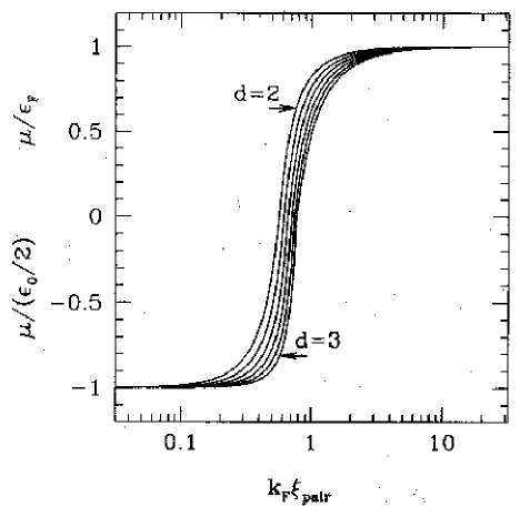
The functions and are shown in Fig. 5, where the gap value attains its maximum at , here . At the same point the value . The symmetry of the functions and about the line reflects the particle–hole symmetry about half-filling. One should consider the hole or anti–particle picture in the region and thus change the sign of the mass . It is also very important (see below) that for small , there is a region where , and that the sign changeover occurs at a definite point .
The expressions that are found in [80, 142] follow directly from (3.25) if, treating as large and the attraction as small, we introduce the 2D two-body binding energy
| (3.26) |
which does not include any many-particle effects. The introduction of the expression (3.26) enables one to take the limit and thus justifies to a certain degree the use of the parabolic dispersion law. In addition the fitting parameter is more physically relevant. For example it is well-defined even for potentials with repulsion. We stress that the introduction of instead of also permits the regularization of the ultraviolet divergence, which is in fact present in the gap equation (3.22).
It should be mentioned that, in a dilute gas model, the existence of a two-body bound state in vacuum is a necessary (and sufficient) condition for a Cooper instability [53, 80, 142]. This statement becomes nontrivial if one considers two-body potentials with short-range repulsion (e.g., hard-core plus long-range attraction), so that one has to cross a finite (but really very weak [151]) threshold in the attraction before a bound state forms in vacuum.
Making use of (3.26), it is easy to simplify (3.25) [53, 80, 142] to
| (3.27) |
where the chemical potential now changes sign at .
To understand the physical significance of these remarkably simple results we look at the two limits of this solution. For very weak attraction (or high density) the two-particle binding energy is extremely small, i.e. , and it is seen that we recover the well-known BCS results with strongly overlapping (in -space) Cooper pairs. The chemical potential , and the gap function .
In the opposite limit of very low particle density (or a very strong attraction) we have a deep two-body bound state , and find that we are in a regime in which there is BEC of composite bosons, or ”diatomic molecules”. The chemical potential here , which is one half the energy of pair dissociation for tightly bound (local) pairs.
It should also be kept in mind that in the local pair regime () the gap in the quasi-particle excitation spectrum equals not (as in the case ) but rather (see [77], the review [53] and the discussion of the Bethe-Salpeter equation in Sec. 3.1.4).
Leaving aside the analysis of for arbitrary values of the parameters (see [141, 54]), let us consider the most interesting case of , with finite . Then finding from (3.26) the expression for and substituting it into (3.20) one obtains
| (3.28) |
Using the potential (3.20) or (3.28) one can demonstrate that the superconducting state is indeed energetically favoured.
3.1.4 Pairs in the Fermi sea
To study the possibility of the existence of the bound states in the presence of a collection of fermions (Fermi sea) the Bethe-Salpeter equation was analyzed in [141]. Here we shall only present the results of this analysis in the particular limit , with finite .111111It is important to stress the difference between the bound states in the vacuum which are always present in a 2D system with attraction and the possibility of existence of such states in the presence of other particles. To analyse the conditions for the existence of bound states in the latter case, the Bethe-Salpeter equation (see, for example, [152]) must be studied. The analysis in [141] showed that if the charge symmetry is unbroken, i.e. , the Bethe-Salpeter energies are given by
| (3.30) |
Thus the system contains non-decaying bound states, i.e. the energies are real, only if . When the solutions acquire an imaginary part which, according to [49], suggests the development of a Cooper instability and vacuum rearrangement.
For the state with the rearranged vacuum so that the analysis of the Bethe-Salpeter equation firstly proved the existence of a gapless Goldstone mode. The second solution of the equation which is only real for is in agreement with the quasi-particle excitation energy described above.
3.1.5 The gradient terms of the effective action and the correlation length versus doping
Now we calculate the terms which contain the derivatives in the expansion (3.17). As before, we shall assume the inhomogeneities of and to be small, restricting ourselves to terms with only the lowest order derivatives. For simplicity we shall also consider the stationary case and calculate only the terms with second-order spatial derivatives. These terms make it possible to determine the coherence length and its doping dependence.
With these restrictions, and taking into account the invariance of (see equation (3.8)) with respect to the phase transformations (3.19), one can write the most general form for the kinetic part of the action as
| (3.31) |
Here there are no items with a total derivative since boundary effects are regarded as unessential, and the coefficients are assumed to be unknown quantities. It follows from (3.31) that, if one includes derivatives up to second order, variations in both the direction (phase) of the field and its absolute value are included.
The calculation for the coefficients is straightforward but rather lengthy. It has been carried out in [141] (see also [54]) using a general method for derivative expansion developed in [153]. The paper [141] also contain the expressions for the case of a finite band-width .
Knowing and one can find the values for different observables. For practical purposes one can restrict oneself to considering the coefficients obtained at the point of minimal effective potential . Instead of and it proves to be more convenient to introduce the combination which determines the change in the value only and arises as the coefficient at . Furthermore, using (3.26) and (3.27), one can derive and in the very simple form:
| (3.32) |
where for completeness we have restored Planck’s constant.
The explicit forms of and permit one to calculate the coherence length and the penetration depth. From Eq. (3.28) one has
| (3.33) |
Then, according to general theory of fluctuation phenomena [154], one obtains
| (3.34) |
This formula shows the dependence of on (or ). The zero temperature coherence length was also studied in [144] for 2D and 3D cases, where it is referred as the phase coherence length .
It is very interesting and useful to compare (3.34) with the definition of the pair size [145, 146] (also sometimes incorrectly referred to as the coherence length (see [142, 143])), namely
| (3.35) |
where
| (3.36) |
is the pair-correlation-function for opposite spins and is the usual BCS trial function. For the 2D model under consideration the general expression (3.35) gives [142, 145]
| (3.37) |
where and are given by (3.27). So, we are ready now to compare (3.34) and (3.37).
Again to understand the underlying physics it is worthwhile to look at the two extremes of (3.34) and (3.37). For high carrier densities, , one finds that , i.e. the well-known Pippard’s result is reproduced correctly. Moreover, if we introduce the pair size in vacuum [80], it is clear that in the high density limit ( and ), . Thus both and prove to be of the order of the pair size, , which is much larger than the interparticle spacing. The latter statement follows from the value of the dimensionless parameter .
In the opposite limit of very low density ( and ) one can see that while . Consequently the correct interpretation of is the pair size (in presence of the Fermi sea (3.35)) rather than the coherence length. The former in the extreme Bose regime is much smaller than the mean interparticle spacing, i.e. , while . The meaning of is the coherence length because it remains finite and comparable with the mean interparticle spacing even in the limit of infinite binding i.e. when goes to infinity. This situation is consistent with the case of 4He where the coherence length is nonzero and comparable with the mean inter-atomic distance although (or energy of nucleon-nucleon binding) is extremely large.
Pistolesi and Strinati in [144] obtained the same results, namely the coincidence of the pair size, and the coherence length in the weak coupling limit and the inequality in the strong coupling or Bose limit . They established that coincides with down to .
The above discussion is a clear example of how the two different energetic scales discussed in [45] behave in the low- and high-density limits. Indeed, the single-particle excitation energy, is obviously related to the individual pair size, , while the energy coherence range is defined by the coherence length, . It follows from the consideration of and above that the energy scales and are the same in the high-density limit. However they diverge in the low density limit where is larger than .
It is interesting to note that the femtosecond time-domain spectroscopy [58] (see also the previous papers on this subject [155] and the papers discussed above [51, 52]) shows the existence of two distinct gaps in the entire overdoped region of Y1-xCaxBa2Cu3O7-δ, where the doping here refers to the chemical fraction of Ca included. It is claimed in [58] that one of them is a temperature-independent “pseudogap” and the other is a -dependent collective gap . They suggest that the presence of two gaps is due to a spatially inhomogeneous picture, supported experimentally by the observation of an inhomogeneous charge distribution [156]. In low carrier density regions is simply the energy scale for single pair formation. In high-density regions one has strong collective effects and a collective temperature dependent gap which shows BCS-type closure at . If such a two-phase picture is indeed correct, then one may have a Fermi surface in that the chemical potential remains positive yet at the same time in local low carrier density regions one can reach the Bose limit – limit of pre-formed pairs.
Another important comment which we have to make here is that the analysis of the experimental data performed in [145] shows that the optimally doped cuprates are definitely on the BCS side of the BEC-BCS crossover in the sense that the chemical potential is close to if one assumes a spatially homogeneous system. To make such a conclusion the ratio was extracted in [145] from the available experimental data for the coherence length. In particular, it was crudely estimated that for YBaCuO with K the ratio ; for BiSrCaCuO with K — and for TlBaCaCuO with K — . It is clear that for a spatially homogeneous model that closeness to the Bose limit implies negative ratio or at least which is apparently not the case for optimally doped HTSC.
Note also that, since and is directly related to the dimensionless ratio , it can be inferred that is another physical parameter which can correctly determine the type of pairing. There is a very remarkable plot from [144], shown in Fig. 6, which examines the behaviour of the dimensionless chemical potential versus ( in the notations of [144]). This plot appears to be quite “universal”, in the sense that it is remarkably independent of the specific model Hamiltonian and of the dimensionality (at least on the mean-field level).121212Notwithstanding these similarities, one should be careful with the Bose limit for the discrete Hubbard model. This limit, as was firstly pointed out in [79], is quite different from that of continuum model (see Sec. 3.3).
The Fig. 6 also shows that the crossover between BCS and BEC regimes occurs in a rather narrow range of the parameter .
Finally, note that the concentration dependence of the penetration depth was also studied in [141] and that the 2D crossover model (3.1) in the presence of a magnetic field was investigated in [157]. In particular the concentration dependence of the derivative was studied and it was shown that [157] this derivative is substantially less in the Bose than in the BCS limit.
3.2 BCS-Bose crossover in the multi-band model: the coexistence of local and Cooper pairs
Clearly the one band model as considered in Sec. 3.1 only describes the part of the phase diagram presented in Fig. 1 corresponding to the superconducting state. Since we have considered zero-temperature we have in fact only described the single left-hand point with zero in Fig. 1. At this point and it thus corresponds to the point in Fig. 5. We will return to possible theoretical explanations for the experimental phase diagram Fig. 1 when we consider the generalization of the one-band model to finite temperature.
There is, however, an important question related to the peculiarities of the crystalline structure of the cuprates. It is known that the La2-xSrxCuO4 system discovered by Bednorz and Müller [1] has K at optimal doping and contains a single CuO2 layer in a cell. On the other hand the later HTSC compound YBa2Cu3O6+δ [158] has K and two cuprate layers per unit cell. The entire homologic family of cuprates has the composition A-M-Ca-Cu-O, where A Bi, Tl, Hg; M Ba, Sr, and the number of CuO2 layers per unit cell, . Since these cuprate layers are situated in the same unit cell the arguments from Sec. 2.2 about the independence of the different CuO2 layers are not applicable in this case (see, for example, a recent paper [159]). Thus the possibility of coherent tunnelling and pairing between such layers must be taken into account. Taken together with the specific features of the BCS-Bose crossover problem discussed in Sec. 3.1, the effect of tunnelling and pairing between adjacent layers in the same unit cell produces rather interesting physics which we will briefly discuss in this section.
Many-band models of superconductivity have been extensively studied in the context of HTSC [162] (see also the review [163]). Here we consider one such model [150] which is directly related to the geometrical structure of cuprates, and with particular emphasis placed on the BCS-Bose crossover.
3.2.1 Model Hamiltonian
Of course, a model which completely reflects the peculiarities of the crystalline and electronic structure of such HTSC materials would be too complicated for consistent calculations. For this reason the following simplifying assumptions were made in [150]: the HTSC material under investigation consists of identical metal blocks separated by spacers; superconductivity emerges in each -layered metal independently so that all the actual interactions are confined to a single block; inside this block, the coupling differs from zero only for the nearest adjacent layers.
Ultimately, we arrive at the Hamiltonian of a multilayered conductor possessing all the above mentioned characteristics (see also Fig. 7):

| (3.38) |
where
| (3.39) | |||||
is the Hamiltonian of free charge carriers and
| (3.40) |
is their interaction.
In Eqs. (3.39), (3.40), the following notation is used: , are the Fermi operators of a particle with an effective mass , spin and from the -th layer satisfying the boundary condition ; is the chemical potential fixing the carrier density ; is a -independent one-particle interlayer tunnelling; are the parameters of the intraplanar and interplanar where the interaction depends only on . Here the sign of the interactions has been chosen such that corresponds to attraction between carriers with opposite spins and we used real time .
The component of the Hamiltonian (3.38) corresponding to the free charge carriers permits diagonalization if we introduce new Fermi fields in accordance with the representation
| ; | |||||
| ; | (3.41) |
As a result, the free Hamiltonian is transformed to the following diagonal form:
| (3.42) |
which describes an -band metal in the effective mass approximation. In this case, a carrier belonging to the -th band is characterized by the effective mass and by the chemical potential
| (3.43) |
The renormalization of mass and the position of each band on the energy scale are determined by the constant of interlayer hopping since , and (a is a parameter having the dimensions of length and associated with the bandwidths in this approximation through the relation ). The chemical potential (3.43) allows us to judge (see Sec. 3.1.3) what type of pairing (i.e. local or Cooper) occurs in the -th band simply by looking at the sign of the corresponding .
In the new variables (3.41) and for local interactions , the interaction (3.40) assumes the form
| (3.44) |
where the matrix element can be expressed directly in terms of the initial parameters . For the sake of simplicity we will retain only the following two values (see above): and . As a result, expressions (3.42) and (3.44) can be regarded as a generalization of the well-known two-band model of superconductivity [160, 161] to the case of an arbitrary number of bands. The symmetry of the chosen model (the equivalence of all planes) and the nature of intra- and interlayer interactions are evident. As an example Eq. (3.44) contains no terms corresponding to interband pairing which generally appear in phenomenological models [162, 163]. Naturally, this does not mean that each band in the model (3.42) and (3.44) behaves independently because the rearrangement of the vacuum (the emergence of anomalous mean values or the condensate) for charge carriers for one of the bands immediately leads to the same rearrangement for charge carriers from the other bands.
As noted previously many-band models of superconductivity have been studied in the context of HTSC [162] (see also the review [163]). The new idea that is brought to the many-band model by using the BCS-Bose crossover formalism is in establishing the correspondence between the sign of the chemical potential of the -th band and the nature of pairs.
3.2.2 Bilayered cuprates
It was mentioned above that bilayered materials include Y-Ba-Cu-O compound. The chemical potentials for the two bands are given by . It proves convenient to introduce the dimensionless constants
| (3.45) |
giving the couplings of the superconducting order parameters from the same and different bands respectively. One may then obtain (see [150]) the following system of equations for the superconducting gaps , and for the chemical potential :
| (3.46) |
If one assumes that intra- and interplanar interactions are the same, i.e. the system (3.46) can even be investigated analytically [150] leading to a better understanding of the underlying physics. Here however we present only its numerical solution shown in Fig. 8.


To avoid confusion with the two gaps and discussed above, we would like to stress that both the gaps and in Fig. 8 are single-particle excitation gaps and have the same origin as . The observation of different gaps in a similar context has been discussed in the literature [164, 165]. It would be interesting to analyze the modern experimental data, for example, [51, 52, 58, 155] bearing in mind that Y-Ba-Cu-O cuprate may have in fact two single-particle excitation gaps.
The behaviour of the chemical potentials shown in Fig. 8 demonstrates a very interesting feature of the many-band model. While for almost the whole range of carrier densities which correspond to the Cooper pair regime in this band, one finds that for a reasonably large range of carrier densities. This means that the pairs in this band are local and one has a coexistence of local and Cooper pairs in the same system. Of course, for higher carrier densities both and become positive and the BCS regime described by the two-band model [160, 161] is restored.
In conclusion it is notable that the idea of mixed BCS vs BEC behaviour in a two gap model of superconductivity was recently readdressed in [166]. In this paper fermions from different parts of the Fermi surface with small and large Fermi velocities respectively were treated as belonging to two different bands.
3.3 Peculiarities of the -wave crossover on the lattice
The physics of the BEC – BCS crossover can be well understood on the basis of continuum models. Nonetheless real superconductors are crystals and, if the pair size is not much larger than the lattice spacing (as in the case of HTSC), lattice effects are important and should be considered.
Let us review the crossover at for the lattice version of the continuum model (3.1), given by
| (3.47) |
where is the transfer integral between neighbouring lattice sites , ; are electronic creation, annihilation operators for the site and spin , respectively, is the strength of the on-site attractive interaction between two electrons occupying the same lattice site, , and is the chemical potential. This Hamiltonian is also called the attractive or negative- Hubbard model. The word “negative” indicates that there is a negative sign before in contrast to the positive sign in the original Hubbard model.
Amongst others, this lattice model defined by (3.47) or (3.49) has been studied in [92, 95, 99, 105, 106, 116] for and in the many other papers mentioned in Sec. 2.3.
The number of charge carriers per lattice site reads
| (3.48) |
where . In momentum representation the Hamiltonian (3.47) can be written as follows
| (3.49) |
Here we have used the notation as an index, is the simplest band energy in the nearest neighbour approximation, we have set the lattice constant , is the number of lattice sites, and is the creation (annihilation) operator for momentum and spin .
We shall predominantly follow the work in [167] and write down the standard coupled equations for the gap and the effective chemical potential 131313Eqs. (3.22) and (3.24) give these equations for the case of a quadratic dispersion law (see (3.15))
| (3.50) |
| (3.51) |
where here (compare with (3.15)) and , where the effective chemical potential is i.e. it contains the Hartree-Fock shift . This shift is essential to ensure that the true chemical potential coincides with in the Bose limit.
The crossover point itself is simply the point where . However, as motivated at the end of Sec. 3.1, it proves physically meaningful to consider the Bose and BCS regions as defined in terms of the pair-size (see Eq. (3.35)) for opposite spin-fermions: the condition identifies the Bose region and the BCS region. From the solution of the equations one can then construct the “phase diagram” [167] (the bound state energy there is denoted as ) shown in Fig. 9 (a) which should be compared to that for the continuum contact potential shown in Fig. 9 (b) considered in Sec. 3.1.

We note that the “phase diagram” for the lattice case is symmetric about half filling . From the diagram it is clear that to obtain a crossover from the BE to BCS regions as one changes the density (at fixed interaction strength ) one needs . In this case the BE and crossover regions occur only at extremely low densities. This is in contrast to the continuum case where one can obtain a density-induced crossover for all coupling strengths. The reason for this difference is the reentrant shape of the curves in the lattice case resulting from the van Hove singularity in the density of states as one approaches half-filling. Note that in contrast for the continuum case the density of states is constant.
One should also note that, in contrast to the continuum case, one cannot always reach the “dilute” boson limit on the lattice at high densities even in the limit of very strong coupling. This effect is not the result of the finite size of the composite bosons which may be regarded as point-like in the infinite coupling limit. Instead it is due to the “overlap” of the centers of mass of the composite bosons since near half-filling the distance between any two bosons is a minimum of a single lattice spacing. Thus one expects the fermionic degrees of freedom to again predominate near half-filling on the lattice [79].
This argument may be quantified [167] by considering the commutator of the following boson-like operator
| (3.52) |
where represents the pair wave function. The commutator may be regarded as a -number provided that the occupation number of each relevant state . This can be achieved at high density (i.e. a large total number of particles) only if there is an infinite number of states available. This condition is clearly not satisfied on the lattice where only a finite number of states exist. Thus, in the lattice case, one must satisfy both the condition and the condition for the system to be regarded as a composite Bose gas.
3.4 Crossover in the models with -wave pairing
In this Section we consider the problem of wave pairing in 2D at zero temperature both in lattice [167, 168, 169, 170, 171] and in continuum models [172, 173]. The motivation for considering this type of pairing is the experimental observation in the ARPES and other measurements [4, 8, 13, 14, 15] of a symmetry in HTSC. We shall analyse the crossover behaviour both as a function of density at fixed interaction strength and as a function of interaction strength at fixed density. The interesting question as to which type of pairing symmetry is actually present as one changes the interaction parameters and the density has been considered in [168, 169, 171] but will not be addressed here.
Firstly one should note that pairs of -wave symmetry cannot contract to point like bosons. This automatically implies that the interaction between composite bosons which results from the Pauli exclusion principle is of finite range. This in turn leads to a larger range of correlations between these bosons which has a dramatic impact on the crossover. In particular at moderately high densities and large couplings these correlations suppress the Bose degrees of freedom and give rise to a larger (fermionic) BCS region [170]. Secondly for the simplest model which permits -wave pairing there exists a critical interaction strength for the formation of a two–body bound state on the empty lattice while this threshold is zero for -wave pairing. This eliminates the possibility for a density induced BCS-BE crossover in this model. Thirdly the -wave symmetry has important implications for both the excitation spectrum and the momentum distribution since at least for the chemical potential greater than the critical (or crossover) value the excitation spectrum is gapless in certain directions.
The lattice models that have been considered are usually 2D Hubbard models. To obtain a -wave solution the fermionic potential must contain an inter-site term of strength in addition to the on-site term of strength considered in the previous section. The Hamiltonian is then given by
| (3.53) |
where corresponds to attraction and the notation denotes as above nearest neighbour pairs. The case of and simply gives the Hubbard Hamiltonian (3.47) which only has an -wave solution. When (inter-site attraction) and (on-site repulsion) one can also find a wave solution of the type
| (3.54) |
We first review the results for this model, the so-called model, with only nearest neighbour hopping and for which the dispersion relation takes the form
| (3.55) |
where is the effective chemical potential
| (3.56) |
which, as in the case of -wave pairing, incorporates the Hartree shift.
In this case there is a critical coupling strength below which no two-body ground state on the empty lattice exists and which gives the start of the BE region at zero density. This is in contrast to the -wave case which has no threshold for pair formation. For a many-body -wave Cooper instability to occur in 2D one needs the existence of a -wave bound state for the two body problem on the empty lattice [53].141414We note that the two-body problem on the empty square lattice was solved many years ago without reference to superconductivity [174] and more fully investigated for the model by Kagan and Rice [175]. However no such condition applies to higher angular momenta and one can therefore obtain a BCS ground state for couplings less than . There is however some controversy as to the minimal coupling strength actually required for such a paired ground state. In [167] it is claimed that pairing always occurs, or equivalently one always has a non-zero value of . As stated in this work [167] this is in direct contradiction to the earlier work of [170] which finds an unpaired region for very weak coupling. In our opinion, the result of [167] is more plausible since the presence of the Fermi surface reduces the dimensionality of the problem [50], and therefore favours the formation of a paired many-body ground state.

For coupling strengths less than no density induced BCS-Bose crossover is possible. For larger couplings strengths, , it is clear from the phase diagram in [170] that one may achieve the crossover point for which crosses the bottom of the band by increasing the density. One cannot however reach a true BCS phase for which by varying density as can be seen in Fig. 10 (a). Thus independent of the coupling strength and in contrast to the -wave case, a density induced crossover is not possible. This is a result of the presence of a pairing threshold [167] as evidenced by considering the model, or extended attractive Hubbard model [103], with second and third neighbour hopping. For this model the dispersion relation is
| (3.57) |
with and and where is again the effective chemical potential given by (3.56).151515This dispersion law captures the small-arc features of the Fermi surface detected in underdoped cuprates. In this case the critical value vanishes for and a density induced crossover is indeed possible as seen in Fig. 10 (b).
For moderate densities, one becomes aware not only of the finite lattice spacing, but also of the intrinsic finite size of -wave bosons. As stated above this finite size enhances the interactions between composite bosons leading to an enhanced fermionic region. For an -wave system one can obtain a crossover from fermionic superconductivity to bosonic degrees of freedom with increasing interaction strength for any choice of the density. For a -wave system such a crossover is only possible in the dilute regime.
One can describe the crossover in terms of the effective chemical potential which is plotted for the model in [170] as a function of the coupling strength for fixed density. Here one confirms that at large doping the chemical potential differs little from its normal state value for a large range of the coupling strength in contrast to both the low-density and the -wave results. The limiting case here is half-filling for which the effective chemical potential is zero, and thus the system is always a fermionic superconductor. It is clear from this work [170] that one can access the crossover point at which the effective chemical potential reaches the bottom of the tight-binding band, albeit at ever increasing coupling strengths with increasing densities, for all values of the density below half-filling. One can never however reach the Bose-limit for higher densities () for both this model and the model [167] since for these densities even for infinite coupling. This is apparent from the line labelled BE in the phase diagrams shown in Fig. 10. This should be contrasted to the corresponding line for the -wave case. It is also confirmed for the model by a plot of the pair-size in the infinite coupling limit as a function of density [170]. From such a plot one can see that the pair-size in the infinite coupling limit even diverges as one approaches half-filling.
The chemical potential also highlights the interactions between the composite bosons in the BE region . In the -wave case the chemical potential approaches minus one half the two-body binding energy in the limit of infinite coupling corresponding to non-interacting bosons. This is only true for -wave symmetry if the density is zero [170, 167]. Defining the boson chemical potential by where is the two-body binding energy its behaviour in the BE region is given by
| (3.58) |
One thus sees that one has for corresponding to an average inter-boson attraction and for corresponding to an inter-boson repulsion which increases with increasing interaction strength (and ).
Returning to the pair-size it can be shown that it does not decrease monotonically with increasing but converges asymptotically to a value larger then the lattice spacing for all . The asymptotic value increases with and diverges as one approaches half-filling. This unusual behaviour is absent in the -wave case and is related to quasi-long-range-order correlations among the bosons which reside individually on nearest neighbour sites. The pair-size in this case measures the correlation between opposite spin fermions belonging to different composite bosons. This can most clearly be seen in the lattice Fourier transform of the pair-wavefunction at half-filling. In the very large coupling limit and at half-filling
| (3.59) |
with lattice Fourier transform
| (3.60) |
where . It decays as a power law with increasing density when is an odd integer and vanishes when is an even integer (including the case for same-site correlation). In contrast in the -wave case the pairing wavefunction tends to a constant with lattice Fourier transform . The divergence of is related to the strong interaction between fermions of opposite spin but on neighbouring lattice sites. It is not related to the divergence of the size of the composite bosons which is related to correlations between fermions of opposite spins but on the same site. For this reason the additional area in the top left of the phase diagrams (Fig. 10) refers to “correlated bosons” (CB) rather than a BCS state even though .
It is interesting to note that the phase diagram shown in Fig. 10 resembles the phase diagram obtained in [177] (see also the review [87]) for the same model, yet taking into account antiferromagnetic ordering competing with superconducting ordering.
-wave pairing has also been considered in the context of a continuum model [173] where the system must be regarded as dilute for the approximations used. For low densities the results are similar to those for the model [170] including the existence of a coupling threshold .
Lastly the -wave symmetry has an important effect on the excitation spectrum and the momentum distribution [173, 170, 176]. The gap parameter is zero at azimuthal angles . Thus for the continuum model with , or the lattice model with above the bottom of the band, the quasi-particle spectrum is gapless at the four Dirac points given by and defined by . Near these points the excitation spectrum is linear. Now consider the direction (or the equivalent directions ) and let denote the energy gap at the point in this direction. The is a non-monotonic function of reaching a maximum at intermediate values of above the crossover point. As reaches the crossover value, becomes zero. The minimal value of the energy gap is thus at the single point and is given by implying that the spectrum disperses quadratically for small momenta for all . As soon as for the continuum model, or (which is physically the same) is below the band edge for the lattice model, the spectrum becomes fully gapped but the minimal gap remains at and takes the value of . This behaviour is strikingly different to that for the -wave superconductor which is always gapped.
Furthermore this behaviour of the excitation spectrum implies that the single particle distribution strength changes dramatically as one passes through the crossover value for for -wave pairing [173, 170, 176]. This discontinuity can be clearly seen in the momentum distribution at which drops to zero discontinuously as the chemical potential crosses the critical value [173]. No such discontinuity is seen in the -wave case. It is also illustrated by the contour plots in [170]). For weak coupling, the chemical potential is essentially equal to its normal state value, and one has a slightly smeared Fermi-surface. The momentum distribution is thus maximal at the centre of the Brillouin zone and falls off least rapidly in the anti-nodal directions . For strong coupling, when the chemical potential has crossed the bottom of the band, the momentum distribution is zero at the centre of the Brillouin zone and has a lobe-like structure centered around and . These directions with high pair occupation probability may well be the preferred direction for the opening of the pseudogap [170].
This qualitative changes in the excitation spectrum and momentum distribution substantially affect the quasi-particle density of states [167]. For low frequencies this is always zero in the -wave case because the system is gapped. For the -wave case it changes discontinuously with from linear in above the crossover value, to a constant at the crossover value, to zero below the crossover value where the spectrum is again gapped.
3.5 Peculiarities of the crossover in models with retarded attraction
As seen in Sec. 2.2 Uemura suggested [84] (see Fig. 4) that the attractive interaction between carriers leading to superconductivity is non-retarded on the Bose side of the BCS-Bose crossover, while on the BCS side the interaction becomes retarded. We could not consider this feature of the Bose-BCS crossover in the previous sections since all the models discussed were based on postulated predominantly local (as in Secs. 3.1 and 3.2) direct non-retarded attraction. It should be admitted that this type of interaction is not realistic and must be regarded as a consequence of a more fundamental interaction whose nature has not yet been established for HTSC. It cannot be ruled out that, as in traditional superconductors, this is the electron-phonon interaction [86] or the electron-magnon (or electron spin-fluctuation) interaction [24] in view of the peculiar magnetic properties of HTSC. In any case in any model describing HTSC correctly, the attraction between charge carriers must be derived from the exchange of excitations of a bosonic field. In such a model, we can not only obtain the attraction between charge carriers, but also estimate the role of such an important factor as the retardation of the interaction. The corresponding generalization introduces one more parameter into the system, viz., the characteristic frequency of elementary bosonic excitations. In low-temperature superconductors, is the Debye frequency for which the inequality is always satisfied. However, in the case of HTSC with a low number density of charge carriers, the situation with is more likely if, for example, optical phonons are responsible for the interaction. Alternatively we can assume that if the interaction is realized through magnons; it might even be the case that (see e.g. [22]).
The inclusion of non-retarded interactions into the Eliashberg equations [182] (see also the textbooks [49, 181, 148] and the review [183]) has been extensively studied and we will give the references shortly. However here we focus on the simplest model with an electron-phonon interaction161616It was noted above that elementary Bose excitations of different kinds may play the role of an intermediate boson, but we will simply refer to them as “phonons”. but with a variable carrier density which makes possible to obtain a BCS-Bose crossover as considered in [178] (see also the more formal treatment in [179]). This is to the best of our knowledge the only attempt to consider the BCS-Bose crossover itself using a model with indirect interaction and we will briefly present the model and discuss the main results. Another related and very interesting question which we discuss here is a possible violation of Migdal’s theorem [180] in HTSC.
3.5.1 Model and basic equations
It is known that (see [152, 181]) the Hamiltonian density describing a system with electron-phonon interaction can be written in the form
| (3.61) |
where is the operator describing phonons with the dispersion ; is a 2D vector; , are the Fermi and Bose fields; is the spin; is the constant of electron-phonon interaction.
In order to clarify the influence of retardation effects on the electron spectrum as a function of , one must analyze a system of two equations. The first equation is the Eliashberg equation [182] (see also the textbooks [49, 181, 148] and the review [183]) for the self-energy of the electron, written in Nambu formalism [147] as
| (3.62) |
where ( being a two-dimensional vector) and one integrates over both the frequency and the momentum. is the vertex function and is the “dressed” phonon propagator.
The second equation is the well-known condition imposed on the Green’s electron function 171717Note that Eq. (3.63) is exactly equivalent to Eq. (3.23) which was written in terms of the effective potential. relating the chemical potential to :
| (3.63) |
Obviously, it is impossible to solve the system of equations (3.62), (3.63) in such a general form, and one must make certain simplifying assumptions.
One such assumption, which is often made in an analysis of the Eliashberg equation, is to disregard effects that are not directly connected to the emergence of anomalous mean values.
The second assumption follows from Migdal’s theorem [180] (see also the textbooks [152, 184, 148]) stating that for , the electron-phonon vertex function can be replaced by its “bare” value . Note that one cannot use directly the result obtained by Migdal since the standard inequality can be violated in HTSC as mentioned above. However, Migdal’s theorem was recently generalized to the case when [185]. Hence the vertex function in (3.62) can also be replaced by in the case of sufficiently low densities (Bose limit) that . Since the results will focus on the Bose and BCS limits, where Migdal’s theorem appears to be valid, one assumes that the “bare” vertex can be used throughout.
It is known [186, 187], however, that the complete vertex should be taken into account for and this consideration leads to a significant increase in . The problem of solving the Eliashberg equation with a vertex correction [187] is very complicated and in fact deserves its own review. Nevertheless, for the limiting cases and considered here, one does not need to include the vertex correction. Nonetheless the final result obtained shows that, if one wants to explain why the BCS regime is not the most optimal for high , one may well need vertex corrections. The theory of the Eliashberg equation with vertex corrections is currently a very rapidly developing branch of superconductivity and we simply mention here some of the latest papers [188, 189, 190, 191] where the relevance of this theory to HTSC and new theoretical developments were discussed.
Furthermore, there is an interesting correlation between the need to include the vertex corrections into the Eliashberg theory and obtaining the correct limiting behaviour in 2D in the study of superconducting fluctuations. For example, it is known that the -matrix approximation which is used extensively (see Secs. 2.3, 4.5) fails to describe BKT physics [95, 135, 92, 102]. At precisely the same time vertex corrections are also crucial.
Finally, the third assumption is associated with the choice of the form of the “dressed” boson propagator. As usual (see [49]), it is replaced by the “bare” propagator [152],
| (3.64) |
In the subsequent analysis, the Einstein model has been used for the phonon dispersion , i.e. . Using this approximation and taking the function to be proportional to the order parameter , one can transform Eq. (3.62) into an equation for the order parameter (see the details in [179]), which depends on the frequency :
| (3.65) |
where again . The problem is thus reduced to an analysis of the system of equations (3.65) and (3.63) as a function of the carrier concentration. It should be emphasized that the Eliashberg equation 3.65 had been investigated and solved several times previously (see e.g. Refs. [49, 152, 181, 182, 192]) but only when the value of coincided with (i.e. one did not consider the BCS-Bose crossover problem). In this latter case the expansion ( is the Fermi momentum) was then used for the normal state spectrum.
3.5.2 Electron spectrum
The desired concentration dependence of the electron spectrum can be characterized by the quantity which defines the energy gap. The system of equations (3.65), (3.63) was studied in [178] using the rather crude approximation that const. It was also studied in [179] by applying a method (see Refs. in [179]) which allows one to reduce the integral Schwinger-Dyson equation (3.65) to a differential one, which can then be solved relatively easily. This more accurate treatment showed good agreement with [178]. Thus here we simply present the main classes of solutions of the system derived in [178]. We assume everywhere that the conduction bandwidth as is appropriate for HTSC.
BCS or high density limit
In the BCS limit, the inequality holds. In this case, it follows from (3.63) that .
a) If we assume that additionally , we reproduce by solving (3.65) the following formula from BCS theory [152]:
| (3.66) |
Thus the above inequality is, as expected, satisfied if the coupling is weak (). Note that Eq. (3.66) corresponds to the result of the classical Morel-Anderson [192] model (if we adopt the notation ). The quantity was obtained in [192] by substitution of a suitably constructed trial function into an equation similar to (3.65) and this represents the first known way of approximating the analytical solution of the Eliashberg equation.
b) If one assumes the opposite limit, , we obtain
| (3.67) |
This result is valid if we assume that the coupling is strong (). If is much greater than , it can be verified that the formula (3.67) corresponds to ultrastrong coupling [193] (see also [181]). Note that to be consistent in this limit the equation for the renormalization factor must also be studied.
Low-density limit
Small values of correspond to the condition . Since the value in this case can be of the order of , Eq. (3.63) becomes nontrivial (see the discussion in Sec. 3.1.3) and does not lead to .
a) If one also assumes that , one arrives at the following solution
| (3.68) |
It can be seen that the condition holds for i.e. weak coupling. Comparing (3.26) and (3.27) with (3.68), one can easily see that the latter equation can be written in the form
| (3.69) |
where
| (3.70) |
Since the expressions (3.70) and (3.26) are similar, it is natural to assume that has the same meaning as defined by (3.26), i.e. is the energy of the bound state which emerges in this case due to the electron-phonon interaction. For this reason, expression (3.70) contains the quantity characterizing the energy of phonons instead of the bandwidth .
At the same time, solution (3.69) differs significantly from (3.27). The latter expression is valid for all values of and all interaction strengths. The former applies only for weak coupling and low densities . If the inequality holds, expression (3.66) must be used. For the charge carriers form an “adiabatically” slow subsystem, and the retardation of indirect interaction can be disregarded as is shown in Fig. 4. However, as the value increases (and especially in the region ), the role of retardation becomes decisive as is evident in formula (3.66).

It can be seen that the asymptotic expression (3.69) for coincides with the numerical solution for , while for and it lies above the corresponding numerical curve (Expression (3.68) can increase without bound, while if one incorporates the band structure then achieves its maximal value at half-filling, see (3.25) and Fig. 5). The maximal value attained is however much lower in the system with an electron-phonon interaction. The gap cannot increase without limit as suggested by Eq. (3.68) but attains a saturation value equal to in the limit .
The chemical potential (which is not shown on the figure) depends linearly on and is negative for very low concentrations of the charge carriers. It can also be seen from (3.69) that for , the chemical potential , and hence the local pair mode is realized (see Sec. 3.1.3). It is important to note that although the quantity was an independent parameter in Sec. 3.1 , in the case under investigation is expressed in terms of electron-phonon interaction parameters. It can be seen from (3.66) and (3.70) that and are connected by the relation , i.e. is exponentially smaller than . Thus in the case of weak coupling, the region of existence of local pairs is very small and is only of theoretical interest.
b) Let us now assume that although , the absolute value of (). In this case one can obtain the following solution of the system (3.65) and (3.63):
| (3.71) |
It can be seen that the condition holds in the strong coupling limit (). In this case, we can again introduce the energy
| (3.72) |
and write the expressions (3.71) in the form
| (3.73) |
Virtually all that has been said about the solution for (3.69) remains in force for (3.73). However, some differences do exist. In particular it can be seen from (3.72) and (3.73) that the region of existence of local pairs is substantially larger in the case of strong coupling.
There is also some evidence that the strong coupling case may be relevant to HTSC due to the presence of an extended van Hove singularity.
3.5.3 Discussion
The results presented here correspond to an oversimplified model. Nonetheless they are a good illustration of the importance of the position of the Fermi level relative to the limiting boson frequency , which is so transparently shown on Uemura’s version of the HTSC phase diagram (see Fig. 4 where an arbitrary boson frequency replaces ). The relationship between carrier density and retardation is clear from the forms of the solutions both in the high density (see Eq. (3.66)) and low density (see Eqs. (3.69) and (3.73)) limits :
| (3.74) |
where is given by from Eq. (3.70) or, for the non-retarded case only, by from Eq. (3.72) respectively.
However, the approximations above have raised certain questions. In particular the quantity and hence attains its maximal value for . The following question thus arises: why do HTSC then attain maximal values of at relatively small values of ? Indeed if one assumes spatially homogeneous systems the presence of real local pairs as suggested by [51, 52] even demands negative . This argument does not apply to spatially inhomogeneous systems. Moreover if one suggests that the optimally doped cuprates correspond to the BCS regime (see Sec. 3.1.5), the model above proposes an explanation as to why this limit gives the highest values.
There also exists a possibility that one can exceed the value of by taking into account the vertex correction for the region [186, 187, 188, 189, 190, 191].
We mention also other recent models [47, 48] with an indirect (through spin fluctuations) interaction between carriers which have been studied recently and where the pseudogap behaviour is the result of a complex interplay between antiferromagnetic and -wave pairing fluctuations. It is very likely that the ultimate explanation of the pseudogap behaviour is only possible within such models. The models with direct interactions between carriers, which we have predominantly discussed here, are only the very first step in understanding the unusual properties of HTSC. However, as we will see in the next chapter there are many unanswered questions even within the relatively simple attractive Hubbard model so often used for the study of crossover and pseudogap behaviour.
4 Self-consistent -matrix approximation and its limitations in the 2D limit
In the previous chapter we considered a number of different models in the mean-field approximation which is of course justified at when continuous symmetry breaking is possible even in 2D [126]. Any generalization of these models to necessarily requires going beyond simple mean-field theory. Here we will describe the different forms of the -matrix approximation widely used to study the Hamiltonian (3.47) or its continuum version (3.1) at nonzero temperatures following mostly the articles [55, 93, 95, 99]. Unfortunately, as we will see in Sec. 4.5, even quite sophisticated approximations may not be sufficient for 2D systems.
4.1 Self-consistent, conserving approximation
We first discuss the -matrix approach to the Hubbard model in the absence of a superconducting condensate i.e in the normal state. The matrix consists of the sum of all particle-particle ladder diagrams (see Fig. 12)
It is known that the -matrix is the ladder approximation to the Bethe-Salpeter equation [184]
| (4.1) |
where is the independent pairing susceptibility given by
| (4.2) |
Recall that , and are the fermionic (odd) and bosonic (even) Matsubara frequencies, respectively. This approximation is expected to be accurate in the low density limit when one can neglect particle-hole scattering and is valid when the product of the Fermi momentum, and the scattering length, is small. Note that the function is chosen to have different signs by different authors (compare, e.g. [95] and [99]), and the reader should take note of the consequence of this sign choice in the subsequent equations.
The corresponding one-particle Green’s function in (4.2) satisfies the Dyson equation (see the diagram in Fig. 13)
| (4.3) |
with
| (4.4) |
where is the electron self-energy.

In the self-consistent -matrix approach the self-energy is given by
| (4.5) |
which closes the system of self-consistent equations.
In most cases the results for real frequencies are obtained from a numerical analytic continuation [194] (see also the review [183]). Since this continuation is inaccurate (see an example in Sec. 7.1.3 and recent comprehensive analysis of the method in [195]) a real-time technique is also used to avoid this problem [99, 100, 104].
The above system of equations, valid in the normal state, is conserving, i.e. satisfying Kadanoff-Baym criteria [89] and “ derivable” in the sense of Baym [88] and known to include Gaussian fluctuations of the pairing field in a self-consistent manner. “ derivable” approximation means that the corresponding self-consistent approximation for the free energy (per lattice site) is given by the functional
| (4.6) | |||||
with
| (4.7) |
and at the stationary point , and are related by Dyson’s equation (4.3) and
| (4.8) |
which reproduces Eq. (4.5). Using short-hand notation one may rewrite (4.6) as (compare with Eq. (3.8))
| (4.9) |
where .
The term “conserving approximation”implies that the approximation conserves the number of particles, the energy, the momentum, and the angular momentum. As proven by Baym [88] “ derivable” theory is conserving [89], although this is not a necessary condition for the theory to be conserving.
In fact the functional (4.6) (or its short-hand form (4.9)) is closely related to the Cornwall-Jackiw-Tomboulis effective potential [196] (see also the textbook [129]) which is widely used in quantum field theory for the description of systems of equations similar to those given here. For example, this method easily permits one to generalize the system (4.1) - (4.5) to a state with a broken continuous symmetry e.g the superconducting state in 3D. Note that such equations were obtained in [97] (see also [90, 98, 101] where these equations were also discussed and solved by different methods) for a 2D model using the functional derivative technique of [88, 89] and solved approximately using a momentum approach.
The electron density as a function of and is given in terms of the thermodynamical potential by
| (4.10) |
If one calculates from and exploits the stationary properties of this functional, one obtains immediately the result,
| (4.11) |
which is equivalent to that given by (3.48) as expected.
The superconducting instability of the normal state at is signalled by the divergence of the -matrix at zero energy (at chemical potential) and zero momentum (the well-known Thouless criterion):
| (4.12) |
This equation, and the associated normal state properties, can be examined in a variety of approximations. Approximations are often used to simplify the fully self-consistent, conserving theory described by Eqs. (4.1) – (4.5), (4.11) since they cannot be studied analytically without additional simplification. However they can be and have been studied numerically [96, 99, 101].
Many of the discussions related to the different predictions and scenarios of these theories, which are all based on superconducting precursor fluctuations, are related to the fact that these additional approximations lead to quite different results (see, for example, the different opinions about the most adequate approach expressed in [55, 57] and [105, 106]). It is thus very difficult to say, at this stage, whether a particular theory really predicts different physics or whether the differences are simply an artifact of the approximation used to solve the -matrix equations.181818There are probably two criteria one can use as a guide to decide which of the existing approaches is the best. Firstly, a good approach should violate as few exact results as possible. Secondly, a good approach should reproduce the exact or numerically accurate results whenever these are known. Based on these criteria the best approach of the -matrix type for the repulsive Hubbard model in the weak and intermediate coupling regimes was probably presented in [135]. We refer the reader to this paper where the generalization of these results to the negative- Hubbard model is also discussed in detail. Our point of view (see Sec. 4.5) is, however, that even in its best form presented in this section, -matrix approximation may not be sufficient for the description of vortex phase fluctuations which are important in the 2D limit at finite temperatures and are the main subject of this review.
4.2 Non self-consistent, non-conserving approximation
The self energy in this case is given by (compare with (4.5))
| (4.13) |
The index “0” indicates the use of free Green’s functions so that the -matrix (4.1) is also calculated in terms of the free Green’s functions
| (4.14) | |||||
The summation over Matsubara frequencies for this lowest order approximation can be easily performed and the -matrix (4.14) is given in terms of the corresponding pair susceptibility (4.2) which acquires a rather simple form
| (4.15) |
with and is the Fermi function.
The full Green’s function in this non self-consistent and non-conserving approximation is the expansion to the first order in the self-energy of (4.3):
| (4.16) |
which means that in (4.16) and (4.13) are not calculated self-consistently.
This system corresponds to the approximation used in the earlier work of Nozières and Schmitt-Rink [79] (see also the reviews [53, 54]) to analyze the BCS-Bose crossover in 3D theory, by solving the system of equation comprising the Thouless criterion (4.12)
| (4.17) |
in terms of given by Eq. (4.15), and the number equation (4.11) (see below its final form given by Eq. (4.18)). In particular, to calculate the fluctuation correction in the number equation (4.11) they replaced by before differentiating. In practice, Nozières and Schmitt-Rink replace the frequency sum in by the standard contour integral representation [49, 148, 184], and deform the contour to lie along the real axis before differentiating with respect to . An alternative (but formally equivalent) procedure is to retain the explicit frequency sum, and to evaluate the derivative by first differentiating with respect to using Eq. (4.8), and then differentiating with respect to . The result is
| (4.18) |
which exactly corresponds to the use of the Green’s function (4.16) defined above. In (4.18) the density is expressed via non-interacting Green’s function .
Note also that the thermodynamical potential
| (4.19) |
which includes the contribution from the sum of all particle-particle ladder diagrams evaluated with non-interacting Green’s functions was firstly studied by Thouless for separable electron-electron interaction [197]. The equivalent representation of this contribution to the free energy is given by Gaussian fluctuations of the pair field in a functional integral representation of the partition function, as was pointed out by Langer [198] (see also the more modern consideration in [149]).
An extension of the Nozières and Schmitt-Rink approach [199] to the case of 2D continuum gas in the same approximation as described here suggested the breakdown of the Fermi-liquid picture for any attraction. Moreover, for any electron density the chemical potential goes to the energy of two particle bound states as in evident contradiction with the results of the mean field theory presented in Sec. 3.1. This specific behaviour of has been associated in [199] with the existence of large bound states in the 2D system mediated by -wave attraction. This was, possibly, one of the earliest papers where the composite hard core bosons were replaced by less stable objects in an attempt to explain the observed properties of cuprate superconductors.
However, the approximation scheme applied in [199] is not sufficient for 2D systems because it is not conserving [93, 116], and neglects the interaction between fluctuations (see also Sec. 4.5). In particular, it was shown in [116] that the values of entropy, and specific heat, become negative in some temperature interval if the thermodynamical potential which leads to the non self-consistent Green’s function (4.16) is used to calculate them. The Green’s function (4.16) even leads to a negative spectral weight, . Indeed, taking given by (4.4) and or simply a function that does not have a zero at , one can see that one of the contributions to coming from the last term of Eq. (4.16) is
| (4.20) |
The derivative of the delta function is negative in certain regions, as one can see by taking one of the many representations of the delta function as the limit of a regular function. In other words, all double poles in result in a negative contribution to the spectral weight. That is one of the reasons why Dyson’s equation (4.3) is necessary: to sum high-order poles to infinite order and transform them into an eigenvalue shift.
All of this represents a serious gaffe of non-conserving, non self-consistent approximation.
4.3 Non self-consistent, conserving approximation
The conserving character of the approximation described in Sec. 4.2 can be, however, restored if we do not expand the Green’s function (4.3) in terms of as we did with Eq. (4.16). At the same time one retains the same approximations for the T matrix (4.14) and self-energy (4.13) so that the Thouless criterion is unchanged and given by Eq. (4.17). This conserving but still non self-consistent approximation was proposed by Serene [93] and the Green’s function in this case is shown diagrammatically in Fig. 14.
As discussed in [93], such an approach entails taking the sum of all repeated scatterings of an electron by independent pair fluctuations, but omitting the interaction between fluctuations and vertex corrections. There is a debate (see, e.g. [93, 116, 99]) as to whether the restoration of the conserving character of approximation will preserve the physics suggested in [199]. Finally we write the number equation (4.11) for the non self-consistent, conserving approximation
| (4.21) |
It is clear that Eqs. (4.18) and (4.21) differ because the first of them is obtained in non-conserving approximation. The two approximations are equivalent when the self-energy corrections are small, but if the corrections are not small, Eq. (4.21) might yield a sensible result when the non-conserving approximation does not.
4.4 Pairing approximation
An alternative approximation to that discussed in the previous section has been used in the set of papers by Levin et al. [55, 56, 57].
The feedback effect of the self-energy on the -matrix has been included into the theory by using the following equation for the T matrix (compare with Eqs. (4.1) and (4.14)):
| (4.22) |
where the full Green’s function is given by the Dyson equation (4.3) and the self-energy is calculated using -matrix (4.22) and the bare Green’s function
| (4.23) |
Thus one can see that the feedback effect is introduced into the theory via the presence of only one full Green’s function in Eq. (4.22). And as usually this system should be completed by the equation for the chemical potential (4.11).
It is stated in [55] that the system (4.22), (4.3), (4.23) and (4.11) is conserving because it satisfies Baym-Kadanoff [89] criteria. It is clear, however, that the theory is not “-derivable” and non self-consistent. Based on the early experimental data which showed the absence of the pseudogap in the optimally doped cuprates it was assumed in [55] that the correct theory should be consistent with BCS theory. Claiming that the fully self-consistent theory discussed Sec. 4.1 does not reproduce the BCS limit in the weak coupling regime (see, e.g. [90, 96]) it was argued in [55] that the mode coupling approach is more appropriate, since it more closely reproduces the results of BCS theory when the coupling is small. More recently however it has become clear that pseudogap phenomena are also observable in the optimally doped region [31], but over a far smaller range of temperatures than for the underdoped cuprates. This implies that one needs reproduce the BCS limit only asymptotically (see Sec. 5.1.2), so that the original objection against the fully self-consistent theory [55] no longer seems valid.
It was also shown in [55] that the mode coupling approximation leads to the desired gap-like self-energy , where is pair-breaking scattering (see Sec. 7.2). However it is stated in [106] that this result is in contradiction with the fully self-consistent theory. This clearly shows that more studies are necessary to determine which approximations are sufficiently good that the results obtained are not simply an artifact of the approximation.
4.5 Limitations of the -matrix approximation
In the previous Section we have discussed the discrepancies between different forms of the -matrix approximation when it is applied to predominantly 3D models. We note also that this approximation neglects the particle-hole channel important for high densities. In 2D there is, however, a more fundamental problem with the -matrix approximation used in any, including the fully self-consistent, form. The essence of the problem is rather well-known: since the superconducting fluctuations are treated in an RPA-like or Gaussian approximation the BKT transition is not recovered by a -matrix approach [95, 92, 135] (see also [200, 201], where the effect of interaction between fluctuations was considered). One may hope however to derive BKT physics, or to be more exact the properties of the system for 191919The region is evidently more complicated due to the presence of vortices which are singular objects. only going beyond the -matrix approximation, e.g. including the equation for the vertex. The -matrix approximation in fact represents only the lowest order approximation to the infinite chain of Schwinger-Dyson equations for the fermion and boson Green’s functions where these have been truncated by neglecting the equation for the vertex function and using the bare vertex. It is known that in the -matrix approximation in the form discussed here there is no BKT solution below the mean-field critical temperature , i.e. there is no solution for the boson propagator behaving like with (see Sec. 6.3).202020Note that studying the Schwinger-Dyson equations one can speak about the BKT phase transition only in terms of the propagators. As was shown in [202] for the 4D gauged Nambu-Jona-Lasinio model solving the equation for vertex leads to the desired behaviour of the boson propagator, but the solution obtained is valid only on the critical line and cannot be analytically continued into a broken phase (which exists in this model). This clearly shows that a more elaborate scheme for the -matrix approximation should be investigated. Note also, in this connection, that the importance of the consistency between the one- and two-particle properties was stressed in [135].
We mention also the recent paper [101] where it is stated that -matrix approximation does not yield the pseudogap behaviour found in quantum Monte-Carlo simulations [108, 109, 110, 111, 112, 113] and always leads to a Fermi-liquid normal state.
At the same time there is some evidence for pseudogap behaviour even for the repulsive 2D Hubbard model, but within a more refined form of the -matrix approximation [135]. If the coupling constant is not too large, one can convince oneself that the spectral weight reveals a two-peak structure near the Fermi level below a crossover temperature, . According to this paper (see also the more recent Ref. [113]) the pseudogap starts to appear (in , but not in ) when the two-particle correlation length becomes larger than the single-particle de Broglie wave length and the system enters into a so-called renormalized classical regime, as confirmed both analytically and numerically. A similar picture applies to pairing fluctuations slightly away from half-filling in the attractive Hubbard model where the pseudogap opens, initially in the region of -space where the Fermi velocity is smallest.
The Gaussian fluctuations destroy long-range order in 2D [128], and if solving equation (4.12) one searches for the at which long-range order sets in, one obtains zero in accordance with the CMWH theorem [126, 127]. In some sense this is an excellent check whether one has a good solution to the -matrix equations: the correct solution should give in 2D.
The most unambiguous acknowledgement of the problem with is evident in [106], where the authors phenomenologically introduce three-dimensionality and define the superconducting critical temperature to correspond to a factor of 100 enhancement of the superconducting susceptibility, i.e. the value of follows from the equation (compare with Eq. (4.12))
| (4.24) |
One can see that this choice of the definition of is entirely arbitrary and with the same success one could propose an enhancement of by a factor of 1000. In fact to avoid problems with the correct definition of most -matrix 2D theories are restricted to the discussion of the phase above and one cannot then investigate the evolution of the pseudogap into the superconducting gap.
There is no doubt that the quasi-2D character of cuprates must be taken into account and many attempts have been made to consider quasi-2D models (see, for example, [27, 56, 65, 203, 204, 205, 206]). However for a pure 2D theory one cannot use the -matrix approach to find the superconducting temperature and we outline an alternative approach in the next chapter.
5 The superconducting transition as a BKT transition and the temperature scale for the opening of the pseudogap
5.1 Phase diagram based on the classical phase fluctuations in the absence of Coulomb repulsion
As discussed in the previous chapter most previous analyses of the behaviour of 2D systems at have been based on different extensions of the Nozières and Schmitt-Rink [79] approach (see, e.g. [199, 93, 200, 201]). This approach, and its -matrix extensions as discussed in Sec. 4.5, do not go beyond the Gaussian approximation for the pairing fluctuations which may explain the abovementioned difficulties faced in these calculations [53]. It is an interesting problem in the theory of superconductivity to develop a finite temperature crossover approach in 2D but based on the BKT transition. Such an analytical treatment did not however prove easy to develop [53].
Nonetheless, there has been some progress using approaches which are specifically designed to deal with the phase degree of freedom. The initial development of the crossover from superconductivity to superfluidity in 2D as a function of the carrier density was carried out as long ago as 1992 by Drechsler and Zwerger [208] (see also Ref. [172], where the -wave case was studied). By means of a Hubbard-Stratonovich transformation a statistical Ginzburg-Landau theory was derived. By applying the correct normalization to make the order parameter a Bose field the following free energy functional results
| (5.1) | |||||
where is the magnetic field, is the speed of light and the effective chemical potential , effective mass and effective coupling strength are all determined by the parameters of the original Ginzburg-Landau theory. The critical temperature must still however be determined by the introduction of a third dimension to avoid divergences in the number equation [208, 157, 172]. It can then be shown that one obtains the correct limiting behaviour for the effective parameters e.g. the chemical potential at the critical temperature attains the value in the Bose limit and in the Fermi limit. Remarkably one also recovers certain features of BKT physics e.g. in the Bose limit the critical temperature is close to the BKT critical temperature for a dilute hard core Bose gas of boson mass and density on a lattice
| (5.2) |
We defer the discussion of the Nelson-Kosterlitz jump in the full (renormalised) superfluid density to Sec. 5.4. As noticed in [117], the method of [208] is fully justified only close to where the linearized Ginzburg-Landau theory is valid. Nor does this method satisfy the important requirement of self-consistency [116].
A crossover theory based directly on the BKT transition which avoids these problems has however been studied in relativistic -theory [207]. We now present this approach which has recently been applied to the theory of superconductivity in a continuum model [115] (see also the generalization to the phonon model (3.61) in [209]). Analogous results, which will also be discussed, have previously been obtained for the discrete Hubbard model [117, 120, 121].
For a 2D system one should rewrite the complex ordering field 212121Because an order parameter is absent in 2D systems we will use this notation in what follows. in terms of its modulus and phase i.e. , as was discussed by Witten in the context of 2D quantum field theory [210] (see also the review [211]), and used in the theory of the superconducting properties of quasi-1D systems [212] and thin films [213]. It is impossible to obtain at finite since this would correspond to the formation of symmetry breaking homogeneous long-range order which is forbidden by the CMWH theorem [126]. However, it is possible to obtain but at the same time due to random fluctuations of the phase (i.e. due to transverse fluctuations of the order field proceeding from the modulus conservation principle [214]). We stress that does not imply any long-range superconducting order (which is destroyed by the phase fluctuations) and, therefore, is not in contradiction with the abovementioned theorem. At the same time one must take into account that is a collective variable which corresponds to some sort of collective behaviour in the 2D system.
The basic concepts that originate from the modulus-phase representation can be summarized as follows. Firstly, as in the paper of [208], one can develop a low-energy theory for the phase fluctuations in terms of an effective model with a superconducting temperature that is given by the BKT temperature [117, 120, 121, 115] (see also [215]). Secondly the amplitude (or modulus) of pairing fluctuations can be non-zero [64, 207, 115, 120, 121, 215] even above the BKT transition temperature and first becomes non-zero at roughly the pairing temperature. We now illustrate these concepts using the simple continuum model of [115] for which one can do much of the calculation analytically and then discuss the effect of the lattice [117] and of quantum phase fluctuations and Coulomb repulsion [120, 121, 215].
We stress that the two concepts above are not specific to the pairing Hamiltonian and/or the BCS-Bose crossover but are related to the dimensionality of the system. Any 2D theory which is characterized by a single complex order parameter has a corresponding effective low-energy theory in terms of the phase of this parameter. The resulting Hamiltonian is often of type with a corresponding BKT superconducting transition temperature. Furthermore the modulus or amplitude of the order parameter can be non-zero above the superconducting transition temperature since this non-zero value does not correspond to long-range order. Thus these ideas were first proposed in a phenomenological model by Emery and Kivelson [25, 26] in which there are two temperature scales as discussed above.
In the continuum model (and in fact in general) three regions can be identified in the 2D phase diagram. The first one is the superconducting (here BKT) phase with at , where is the temperature of the BKT transition, which plays the role of in pure 2D superconducting systems. In this region there is algebraic order, or a power law decay of the correlations. The second region corresponds to a phase with non-zero (), where is the temperature at which the homogeneous (by definition) becomes zero. In this phase although is still non-zero the correlations mentioned decay exponentially. The third is a normal (Fermi-liquid) phase at where .222222It might be the case that never becomes strictly zero. In this case one would have crossover behaviour instead of a phase transition, see, for example, P. Curty, H. Beck, Phys. Rev. Lett. 85 (2000) 796. Note that everywhere as is the case for all other correlators which violate the symmetry e.g. . Note that while this phase diagram was derived for the idealized 2D model, there are indications that even in layered systems as complicated as HTSC the critical temperature may nonetheless be well estimated using [64, 204], even though the transition undoubtedly belongs to the 3D class (see also [216]). The identification of the intermediate phase with the pseudogap phase is somewhat controversial and we will return to this point in some detail. We note however that it has been pointed out by Abrikosov [64] that a nonzero gap in the one-particle excitation spectrum can persist even without long-range order, being a local characteristic (see the discussion in Sec. 6.1).
The proposed description of the phase fluctuations and the BKT transition is of course very similar to that proposed earlier by Emery and Kivelson [25, 26]. However in their phenomenological approach the field does not appear explicitly while in the present microscopic approach it occurs naturally. We mention here also the application of similar ideas to the 3D case [216], where instead of the 2D temperature one has the temperature of the phase transition in the 3D -model, .
There is no need to write down the model Hamiltonian which is studied here, since it is identical with that described in Sec. 3.1.
The desired phase diagram consisting of normal, anomalous and superconducting phases was calculated in [115] employing the Hubbard-Stratonovich method (see Sec. 3.1.1, the equations (3.6) – (3.8)). In the 2D case at nonzero , however, instead of using the accepted method for the calculation of the partition function (see (3.6)), one must perform the calculation in modulus-phase variables. This allows one to avoid any subsequent treatment of the phase fluctuations at Gaussian level only. Thus, one is able to take into account the phase degree of freedom with the needed accuracy.
The modulus-phase variables were introduced in accordance with [217], where the parameterization
| (5.3) |
was used. At the same time as this replacement (5.3) is implemented, one makes the gauge transformation
| (5.4) |
[210] (see also Refs. [211, 213, 217]). Physically, this amounts to replacing the charged fermion with a neutral fermion and a spinless charged boson . These parameterizations, (5.3) and (5.4), prove more appropriate for presenting the corresponding functional integral in two dimensions [210]. In Nambu variables (3.2) the transformation (5.4) takes the following form
| (5.5) |
Note that the neutral fermion variables are still Grassmann fields since they satisfy the appropriate anti-commutation algebra.
Making the corresponding substitutions (5.5) into the representation (3.6) and integrating over the fermi-fields and we arrive at the expression (compare with (3.7) and (3.8))
| (5.6) |
where
| (5.7) |
is, as (3.8), the one-loop effective action, which, however, depends on the modulus-phase variables. The action (5.7) is expressed through the Green’s function of the initial (charged) fermions that has in the new variables the following operator form232323It may be obtained as a solution of a differential equation with anti-periodic boundary conditions (see (3.9) and (3.10)).
| (5.8) |
with
| (5.9) |
The free fermion Green’s function provides a convenient regularization in the process of calculation. It is important that neither the smallness nor slowness of the variation of the phase of the order parameter is assumed in obtaining expression (5.7). In other words, it is formally exact.
Since the low-energy dynamics of phases for which is governed mainly by long-wavelength fluctuations of , only the lowest-order derivatives of the phase need be retained in the expansion of :
| (5.10) |
where
| (5.11) |
and
| (5.12) |
The kinetic and potential parts can be expressed in terms of the Green’s function of the neutral fermions, which satisfies the equation
| (5.13) |
and the operator (5.9).
The representation (5.10) enables one to obtain the full set of equations necessary to find , , and at given (or, for example, and at given and ). While the equation for will be written using the kinetic part (5.11) of the effective action, the equations for and (or and ) can be obtained using the mean field potential (5.12). It turns out that in a phase for which , the mean-field approximation for the modulus variable describes the system quite well. This is mainly related to the non-perturbative character of the Hubbard-Stratonovich method, i.e., most of the pairing effects are included in the nonzero value of .
It is clear that the CMWH theorem [126] does not preclude nonzero and, as a consequence, an energy gap for fermion , since no continuous symmetry is broken when such a gap appears. Despite strong phase fluctuations in the two-dimensional case, the energy gap in the spectrum of the neutral fermion still persist in the spectrum of the charged fermion (see Chap. 7 and [125]), even well above the critical temperature.242424We note that the specific heat experiments [4, 107] demonstrated a loss of entropy at temperatures much higher than . This can be considered indicative of a degenerate normal state, consistent with the existence of a nonzero order parameter .
Thus, within the proposed scenario, the pseudogap properties might conceivably be attributable to the energy gap of a neutral fermion introduced in the way described above, so that the pseudogap itself can be considered as a remnant of the superconducting gap. The condensate of neutral fermions is completely unrelated to the superconducting transition; the latter is only possible when the superfluid density of bosons becomes large enough to stiffen the phase . The temperature at which nonzero develops should be identified in this approach with the pseudogap onset temperature (see Sec. 5.1.2 item a and the discussion about heavily underdoped region in Sec. 5.1.3).
The strategy of treating charge and spin degrees of freedom as independent seems to be a useful, and at the same time general feature of two-dimensional systems [210, 213] and low-dimensional systems in general (see also the review [218]).
5.1.1 Derivation of self-consistent equations for , neutral order parameter, and chemical potential
When the model under consideration is reduced to some known model describing the BKT phase transition, one can easily write down an equation for , which in the present approach can be identified with the superconducting transition temperature . Indeed, in the lowest orders the kinetic term (5.11) coincides with the classical spin -model [130, 131, 132, 133, 134], which has the continuum Hamiltonian
| (5.14) |
Here is the some coefficient (in the original classical discrete -model it is the stiffness of the relatively small spin rotations) and is the angle (phase) of the two-component vector in the plane.
The temperature of the BKT transition is, in fact, known for this model:
| (5.15) |
Despite the very simple form of Eq. (5.15), it was derived (see, e.g., Refs. [130, 131, 132, 133, 134]) using the renormalization group technique, which takes into account the non-single-valuedness of the phase . Thus, fluctuations of the phase are taken into account in a higher approximation than Gaussian and this approximation may well be better than the -matrix even in its fully self-consistent conserving form. However, the disadvantage of such an effective theory of the phase fluctuations is that one loses contact with the underlying fermions (they are essentially integrated over to obtain the effective theory252525This contact, however, would not be lost if one retained the source terms for the fermi-fields in the corresponding functional integral. See also the approach of [124] where the low energy fermions are not integrated out.). From this point of view, these two approaches are essentially complementary.
The -model was assumed to be adequate for a qualitative phenomenological description of the underdoped cuprates [25, 26, 27] (see also Refs. [66, 120, 221]), and the relevance of the BKT transition to Bose- and BCS-like superconductors was recently discussed in Ref. [172] (see also [222]). The most important difference between superfluidity in 4He films, which is adequately described by the -model [130], and superconductivity is that the superconducting liquid is charged. This results in coupling to the magnetic field, which inevitably accompanies any current flow in the superconductor, e.g. in the presence of vortices. However, as was shown in [222, 172] the effective penetration depth for the magnetic field in thin films is of the order of 1 cm, and thus for sample sizes smaller than this, magnetic screening becomes irrelevant. In such a situation the difference between charged and neutral superfluids becomes irrelevant and superconducting films may undergo the BKT transition. Note also that this difference leads also to electric coupling between Cooper pairs, in particular those situated in different superconducting layers. The effect of this coupling is considered below in Sec. 5.3.
To expand up to , it is sufficient to restrict ourselves to terms with in the expansion (5.11). The calculation is similar to that employed in [217], where only high densities were considered at . (We mention also the derivation of the effective action at in [223] where the fluctuations in the density (conjugated to the phase ) were also treated.) Thus, to obtain the kinetic part, one should directly calculate the first two terms of the series (5.11), which can be formally written and . We note that has the structure , where and are differential operators (see (5.9)). One can see, however, that the part of proportional to the unit matrix does not contribute to . Hence,
| (5.16) |
where (compare with (3.15))
| (5.17) |
is the Green’s function of neutral fermions in the frequency-momentum representation, with and defined after (3.15). The summation over the fermionic Matsubara frequencies and integration over in (5.16) can be easily performed using the sum (A.7); one thus obtains
| (5.18) |
where
| (5.19) |
This has the form of a Fermi quasi-particle density (for the expression (5.19) is simply the density of free fermions given by the first term in (4.18)).
For the case [217], in which the real time replaces the imaginary time , one can argue from Galilean invariance that the coefficient of is rigorously related to the coefficient of . It therefore does not appear in . We wish, however, to stress that these arguments cannot be used to eliminate the term from when , so that we must calculate it explicitly.
The term in yields
| (5.20) | |||||
Using (A.11) to calculate the sum over the Matsubara frequencies, we find that
| (5.21) |
where
| (5.22) |
Obviously, the term does not affect the coefficient of . Further, it is easy to make sure that the cross term involving and in is absent. Finally, calculations of the contribution to yield262626 Derivatives higher than were not found here.
| (5.23) |
Thus, summing over the Matsubara frequencies (see Eq. (A.12)), one obtains
| (5.24) |
As expected, this term vanishes when , but at finite it is comparable with (5.18).
Combining (5.18), (5.24), and (5.21) we finally obtain
| (5.25) |
where
| (5.26) |
characterizes the phase stiffness and governs the spatial variation of the phase . One can see that the value of the phase stiffness coincides with the nonrenormalized stiffness used in Ref. [25].
During the derivation of the effective action for the phase field we have neglected the so-called Landau terms (see [224] and Refs. therein) which have a non-local form and thus cannot be presented in terms of the derivative expansion. These terms are important since they make the -mode decaying for any . However, as recently shown in [224], for -wave superconductors their contribution is negligible at least for . This is not the case for -wave superconductors where these terms are expected to be important even in the low temperature region.
The quantity vanishes at , which means that above the modulus-phase variables are meaningless; to study the model in this region one must return to the old variables and . Near one can obtain from (5.26) in the high-density limit (see below)
| (5.27) |
where is the zeta function.
Direct comparison of (5.25) with the Hamiltonian of the -model (5.14) makes it possible to write Eq. (5.15) for directly:
| (5.28) |
Although mathematically this reduces to a well-known problem, the analogy is incomplete. Indeed, in the standard -model (as well as the nonlinear -model) the vector (spin) subject to ordering is assumed to be a unit vector with no dependence on . In this case this is definitely not the case, and a self-consistent calculation of as a function of requires additional equations for and , which together with (5.28) form a complete set. We note, however, that the dependence of on was neglected in [25], where the nonrenormalized phase stiffness was used to write Eq. (5.28). Using this nonrenormalized phase stiffness one would obtain that which is, as we will see, apparently wrong for high carrier densities since one does not recover the BCS limit.
Using the definition (5.12), one
can derive the effective potential
(see Appendix A).
Then the desired missing equations are the condition
that the potential (A.10) be minimized, and the equality
, which
fixes .
These are, respectively
(compare with Eqs. (3.21) – (3.24))
| (5.29) |
| (5.30) |
where is defined by (5.19).
Equations (5.29) and (5.30) comprise a self-consistent system for determining the modulus of the order parameter and the chemical potential in the mean-field approximation for fixed and .
It is very interesting to note that to resolve the problems which are present in the non-conserving, non self-consistent approach (see Sec. 4.2), the following form of the phenomenological pair susceptibility (compare with Eqs. (4.2) and (4.15)) was suggested in [116]
| (5.31) |
where is a function with a free parameter , and has the form (compare with (5.19))
| (5.32) |
It was stressed in [116] that is not an off diagonal long-range order parameter but is related to pair binding. The phenomenological susceptibility (5.31) was then used in [116] to write down the thermodynamical potential (see 4.6) where (see 4.7) is given in terms of (5.31). This thermodynamical potential was then used to derive equations for the chemical potential (which coincides with (5.30)), entropy and specific heat. An additional equation for was derived in [116] by minimizing this potential with respect to subject to the number constraint . It was shown in [116] that the presence of avoids problems with negative entropy and specific heat which are present in the non-conserving, non self-consistent approximation discussed in Sec. 4.2.
Eqs. (5.29) and (5.30) seem to yield a reasonable approximation at high densities , since they include the condensed boson pairs in a non-perturbative way via nonzero . Nonetheless they must certainly be corrected in the strong coupling regime (low densities ) to take into account the contribution of noncondensed bosons (this also appears to be important for Eq. (5.28), which determines ). The extent to which this alters the present results is not completely clear. Previously, the best way to incorporate noncondensed pairs appears to have been the self-consistent -matrix approximation (see e.g. [55, 91, 93, 95] and other references in Secs. 2.3 and 4), which allows one to account for the feedback of pairs on the self-energy of fermions. However as we discussed above, the -matrix approach, at least in its standard form presented in Sec. 4, fails to describe the BKT phase transition, for which one must consider the equation for the vertex. On the other hand, in this approach the BKT phase transition is realized by the condition (5.15), while an analog of the -matrix approximation in terms of propagators of the -particle and the neutral fermion has yet to be developed.
Again the energy of two-particle bound states in a vacuum defined by (3.26) is more convenient to use than the four-fermion constant . For example, one can easily take the limits and in Eq. (5.29), which after this renormalization becomes
| (5.33) |
Thus, in practice, we solve Eqs. (5.28), (5.30), and (5.33) analytically and numerically to study as function of (or equivalently, of the Fermi energy ). It is easy to see that at , the system (5.30), (5.33) transforms into a previously studied system (3.29). Setting in Eqs. (5.29) and (5.30), we obtain (in the same approximation) the equations for the critical temperature :
| (5.34) |
where ( is the Euler’s – Mascheroni’s constant) and the corresponding value of :
| (5.35) |
Note that these equations coincide with the system that determines the mean-field temperature and , evidently as a result of the mean-field approximation for the variable used here. Thus in this approximation the average amplitude of the pairing fluctuations is simply given by the mean-field gap which is non-zero below (). This non-zero amplitude then plays the role of the “pseudogap”. Note that the paramagnetic susceptibility (see [115]), specific heat in the mean-field approximation exhibit kink-like behaviour at while at the superconducting transition temperature they do not show any singularities. The picture presented here is thus to all practical purposes identical to that given in [120, 121].
There is an important difference between the temperatures and . Specifically, if one takes fluctuations into account, goes to zero, while the value of remains finite. The crucial point is that the perturbation theory in the variables and does not contain any infrared singularities [210, 219], in contrast to the perturbation theory in ; thus the fluctuations do not reduce to zero. This is why the temperature can have a physical meaning: incoherent (local or Cooper) pairs begin to form (at least at high enough , see Secs. 5.1.2 item c and 5.1.3) just below . At higher temperatures, only pair fluctuations exist (see, e.g. [220]).
5.1.2 Main results
The interested reader may find a more detailed discussion of the results for the continuum model in [115]. Here we present only the issues directly related to the phase diagram of the model (3.1). A numerical and analytical investigation of the systems (5.28), (5.30), (5.33), and (5.34), (5.35) yields the following results, which are displayed graphically as the phase diagram of the system.
a) For rather low carrier densities, the pseudogap phase area (see Fig. 15) is comparable with the BKT area.

For high carrier densities (), inserting into (5.27) the well-known dependence of (see, for example [49])
| (5.36) |
and then substituting (5.27) into (5.28) one obtains the following asymptotic expression for the BKT temperature (also given in [222, 107, 216] and [209], where the corresponding asymptotical expression for the boson-exchange model (3.61) was obtained)
| (5.37) |
which shows that the pseudogap region shrinks asymptotically. This behaviour qualitatively restores the BCS limit. This is a good place to consider the difference between the two high-density limits shown in Fig. 2-A and -B respectively. As one can easily see, Eq. (5.37) implies that the present results are in favour of the picture presented in Fig. 2-B.272727Of course, does not reach zero at high doping due to the oversimplified character of the model. For example, we saw in Sec. 3.1 that may decrease due to band filling or at the very least stabilizes as in the model with phonon interaction from Sec. 3.5. Nonetheless one clearly sees that and are merging. The merger of and in the approach based on the superconducting fluctuations is probably not that surprising since both these temperatures have the same superconducting origin. However, as one can see from Fig. 2-A this merger would be rather unusual if one accepts the antiferromagnetic pseudogap scenario and considers to have a magnetic nature, different from that of . Thus, as was suggested in [23], additional studies on the overdoped cuprates in a magnetic field may also help to clarify the pseudogap origin.
It has been shown that for optimal doping, the dimensionless ratio can be estimated as [146]. This implies that the size of the pseudogap phase predicted by (5.37) to be of order [222, 107, 216] is (even in the underdoped region) much smaller than the difference observed in cuprates. One might however be able to explain this discrepancy either by the presence of impurities as done in Sec. 5.4 or by the formation of spatial inhomogeneities e.g. stripes.
b) For , the function is linear, as is confirmed by the analytic solution of the system (5.28), (5.30), and (5.33), which yields . As we discussed in Sec. 2.2 (see also the Uemura plot in Fig. 3) such behaviour of is observed for all families of HTSC cuprates in their underdoped region though with a smaller coefficient of proportionality (). Again this discrepancy can be in principle explained by the presence of non-magnetic impurities (see Sec. 5.4). Other reasons such as, for example, a contribution due to noncondensed pairs in Eq. (5.28) which defines , could also be important.
c) Finally the calculations showed (see Fig. 16)

that the ratio for the carrier densities shown in the figure is greater than 4.7 and grows as the doping decreases. This result is also confirmed by the more general consideration of Abrikosov [64] which is also based on phase fluctuations of the order parameter but takes into account interlayer tunnelling. This concentration behaviour is consistent with numerous measurements of the ratio in HTSC [4]. The value is, however, somewhat lower and reaches the BCS theory limit of 3.52 only for . It is very interesting and important that the measurements of [32] show that for all doping levels which is very close to the BCS value, but for a -wave superconductor. This presents a strong argument in a favour of the theories which relate the pseudogap formation at to the precursor superconducting fluctuations. In this case the scale for is the BCS temperature , or as in [115] which, as we showed, has a quite rigorous definition in the modulus-phase approach. Another important conclusion which one can draw from the experimental values of [32] is that the simple Bose-BCS crossover theories with pre-formed local pairs existing in the region with (or even ) with are unable to give since Fig. 16 clearly shows that the ratio grows for very low carrier densities. As we discussed in Sec. 3.1.5 one may still have local Bose pairs in a more sophisticated picture where the system is inhomogeneous (see also the discussion in Sec. 5.4 about the differences between the approaches of Uemura [84] and Emery-Kivelson [25, 26]).
Note also that the divergence of and at is directly related to the definition of at .
5.1.3 Pairing temperature versus carrier density. More about the meaning of
There is no disagreement concerning the asymptotic behaviour of (or shown in Fig. 1) proportional to in the region of very low carrier densities. In contrast, the behaviour of the temperature , below which we assumed pairs are formed, cannot be considered to be generally accepted. It is an open question as to how it behaves in the heavily underdoped cuprates: namely whether it increases being related to the Néel temperature or decreases. The opinion of theoreticians on this subject is also divided.
For example, on the phase diagram suggested by Uemura in Fig. 4, the temperature is taken to be the temperature of local uncorrelated pairing which increases with decreasing . Randeria (see Ref. [53] and references therein), to define the pairing temperature , uses the system of equations for the mean-field transition temperature and the corresponding chemical potential, which is essentially identical to the system (5.34), (5.35). Thus his as . This is accordance to the behaviour of shown in the theoretical phase diagram from Fig. 1 suggested by Zachar [23].
It is also well known [53, 90, 199] that in the low-density limit, it is vital to include quantum fluctuations, at least in the number equation [79], in the calculation of the critical temperature at which long-range order forms in 3D.
Certainly quantum fluctuations are also important in the calculation of in the limit and, in particular, in the number equation. However, as already stressed in Sec. 5.1.1, these corrections are quite different from that obtained using the variables , since perturbation theory in the variables and does not contain any infrared singularities [210, 219], and the fluctuations do not yield .
In our opinion, the temperature has its own physical interpretation: this is the temperature of a smooth transition to the state in which the neutral order parameter , and below which one can observe pseudogap manifestations. In this respect the temperature can be compared with the crossover temperature introduced for the repulsive and attractive Hubbard models in [135] (see also the explanation in Sec. 4.5). At the same time note that both these temperatures should not be strictly identical to the mean-field temperature (see the end of Sec. 5.1.1).
There is also a very interesting and important question about the character of the transition (see, for example, [215]). Certainly in the simplest Landau theory one appears to have a second-order phase transition, since takes a nonzero value only below [207] and since has only been treated in the mean-field approximation i.e. one has neglected the fluctuations in both and , a second-order phase transition was obtained at . However, as it was stressed in Introduction, experimentally the formation of the pseudogap phase does not display any sharp transition and the temperature observed in various experiments is to be considered as a characteristic energy scale and not as a temperature where the pseudogap is reduced to zero [4, 31]. We believe that taking into account the fluctuations of may resolve the discrepancy between the experimental behaviour of and the temperature introduced in the theory.
To define the temperature properly, one should study the spectrum of bound states either by solving the Bethe-Salpeter equation [141] (see also Sec. 3.1.4) or by analyzing the corresponding Green’s functions as is done here. It turns out that there is no difference between and in the Cooper pair regime (), while in the local pair region () these temperatures exhibit different behaviour.
Indeed, let us study the spectrum of bound states in both the normal () and pseudogap () phases. We are especially interested in determining the conditions under which real bound states (with zero total momentum ) become unstable. For this purpose one can look at the propagator of the -particle in the pseudogap phase:
| (5.38) |
where is defined by the minimum condition (5.29) (or (5.33)) of the potential part (A.10) of the effective action (5.7). In the momentum representation, the spectrum of bound states is usually determined by the condition
| (5.39) |
where is the retarded Green’s function obtained directly from the finite temperature Green’s function (5.38) in frequency-momentum representation, using analytical continuation . Recall that such analytical continuation must be performed after evaluating the sum over the Matsubara frequencies. In the case of vanishing total momentum , one arrives at the energy spectrum equation
| (5.40) |
From the explicit expression (5.40) for , this function obviously has a branch cut at frequencies
| (5.41) |
Thus, bound states can exist only below this cut.
Real bound states decay into two-fermion states when the energy of the former reaches the branch point . Since is a monotonically decreasing function of , the solution for the bound-state energy must be unique and is given by . At this point Eq. (5.40) coincides exactly with the mean-field equation (5.29) for so that takes on the mean-field value. It is also clear that for we have real bound states with energy below the two-particle scattering continuum at , while at there are no stable bound states. The line in the – plane at separates the negative region, where local pairs exist, from that in which only Cooper pairs exist (positive ). This line (see Fig. 17) begins at the point , and ends at , . (The latter follows directly from the solution at given by (3.27).)

To find the equivalent line in the normal phase with i.e. above , we consider the corresponding equation for the bound states. The propagator of these states (in imaginary time formalism) is defined to be
| (5.42) |
(In the normal phase, where , we must again use the initial auxiliary fields and .) Then in the momentum representation (after summing over the Matsubara frequencies) we have
| (5.43) | |||||
where is the relative momentum of the pair. It is seen that Green’s function (5.43) coincides with the -matrix (compare with Eqs. (4.14) and (4.15)) in the non self-consistent, non-conserving approximation, up to an overall minus sign. The spectrum of bound states is given again by Eq. (5.39). Using the energy (see Eq. (3.26)) of the bound state at , for we obtain the following equation for the energies of these states in the normal phase:
| (5.44) |
Such states can exist provided . The left-hand side of Eq. (5.44) is positive at and tends to () or () when . This equation thus always has a solution between and for , i.e. bound states with zero total momentum exist for negative .
For , the analytic analysis becomes more complicated, and requires numerical study. One can easily find from (5.44) that for the special case , which is not in fact in the normal phase but for which one can use the variables and , that such stable bound states exist up to (see also proof in Sec. 3.1.4). In fact, numerical study for shows that the trajectory (or , see (5.35)) approximately divides the normal phase into two qualitatively different regions – with () and without () stable (long-lived) pairs. This result is the same as that in the phases with , so that the line (Fig. 17) separates the regions with stable and unstable pairs for all non-zero temperatures. However this line (squares) does not correspond to any phase transition.
Given the two-particle binding energy as a function of temperature, it is natural to define the pairing temperature by . This equation can be easily analyzed in the region , for which we directly obtain , which clearly coincides with the standard estimate [84, 95]. This means in turn that the curve starting at will decrease until the point , which lies on the line (see Fig. 17). It is important that this line is not a phase transition curve; it merely divides the fermion system diagram into temperature regions where one has either a prevailing mean number of local pairs () or unbound carriers (). This is the region of the abnormal normal phase where one has some density of pre-formed boson pairs. It is widely accepted, however, that this case is only of theoretical interest, since there is no Fermi surface () in this phase (see nevertheless the discussion in Secs. 1.3, 3.5.3 and Refs. [51, 52, 42, 43]). The phase area or the difference is an increasing function as , which corresponds to the behaviour usually assumed [84, 25].
When there are no stable bound states () in the normal phase. Formally, using in Eq. (5.40), we immediately obtain (5.34) or, in other words, here . Such a conclusion is in accordance with the generally accepted definition of in the BCS case [95].
Thus the phase diagram of a 2D metal above acquires the form shown in Fig. 17. It is interesting that if there are no stable pairs i.e. is not well defined, then the temperature is the line below which pairs reveal some signs of collective behaviour. Moreover, for one can speak of a real pseudogap in the one-particle spectrum, while in the region only strongly developed pair fluctuations (a finite number of pairs) exist, although they probably suffice to reduce the spectral quasi-particle weight, and to produce other observed manifestations that mask pseudogap (spin gap) formation.
5.2 The peculiarities of the phase diagram for the lattice model
The discrete version of the attractive Hubbard Hamiltonian (3.47) was also mapped [117] into the classical -model. Although we disagree on some of the fine points in the derivation we agree entirely with the results. It is instructive to consider these fine points since they yield a better understanding of the modulus-phase formalism described in Sec. 5.1. The statistical sum (3.7) is written in [117] for (3.47) in the momentum representation. Then the saddle-point approximation described by (3.12) is considered. Of course, this approximation leads to nothing but the finite temperature generalization of the zero temperature equations for (3.21) and (3.23) considered in Sec. 3.1.3. The value in these equations is called in [117] “order parameter” in accordance with the saddle-point character of the derived approximation for the complex Hubbard-Stratonovich fields and . These equations are, of course, formally identical to Eqs. (5.29) and (5.30) derived in Sec. 5.1.1, but as we have discussed the meaning of is completely different allowing nonzero but keeping .
To go beyond the saddle-point approximation, it is proposed in [117] to consider a variation of the Hubbard-Stratonovich fields around their saddle-point values. In doing this, one looks for the low energy excitations. It is claimed in [117] that choosing the order parameter to be real (or taking it any specific value), one breaks its continuous symmetry, provided . According to Goldstone’s theorem, this symmetry breaking implies that a soft mode exists as . These modes are associated in [117] with the phase fluctuations of the order parameter. It is clear, however, that this breaking of the continuous symmetry and appearance of the Goldstone mode in 2D at are strictly forbidden by the CMWH theorem [126]. In fact the above conclusions of [117] are obviously related to the use of the saddle-point approximation in the form described in Sec. 3.1.1. To be consistent with the CMWH theorem one should (following by Witten [210]) use the set of transformations (5.3) and (5.4) for any 2D theory. As we have explained in Sec. 5.1 these transformations make the perturbation theory in the modulus-phase variables free from symmetry violating terms. Furthermore, as we will see in Sec. 6.3 in 2D the propagator associated with the phase fluctuations does not have the canonical behaviour and becomes softer.
All these comments do not however change the results of the calculations in [117] but rather reflect subtle points in their interpretation. Thus we present the effective action for the phase mode derived in [117]282828Note that the phase was assumed to be time-independent in [117].
| (5.45) |
with
| (5.46) |
where is the solution of the mean-field gap equation (see e.g. Eq. (5.29)), the subscript indicates , , , and is the usual Fermi functions with . As in Sec. 5.1.1 one may check that is nonzero only below the mean-field (BCS) critical temperature where .
To provide a link with the -model, one expands up to second order in to obtain the low energy behaviour
| (5.47) |
This expansion of in momentum space is an equivalent way to understand the approximations used in the derivative expansion in Sec. 5.1.1. Note that the definition of the phase stiffness used here and in Sec. 5.1 differ by a factor of 2. The effective model is then discretized in [117] by introducing a lattice parameter :
| (5.48) |
where is the dimensionality of the system.
One can also derive an effective -model starting from the Ginzburg-Landau theory [203, 208, 172]. As noticed in [117], this procedure which allows one to write parameters of the effective -model in terms of the Ginzburg-Landau parameters, is only fully justified close to where the linearized Ginzburg-Landau theory is valid. However, as we saw in Sec. 5.1.2 the most interesting region i.e. that with a relatively large pseudogap corresponds to (or ) which is clearly beyond the limits of validity of the Ginzburg-Landau theory.
Arguing that the phase stiffness is only weakly temperature dependent up to a temperature of the order of the BCS temperature it was suggested in [117] to use
| (5.49) |
where and . The low temperature value of as a function of is shown in Fig. 18. One can see that for large , goes as .
Assuming a rectangular density of states of width (i.e. a square band extending from to ) and an electron density consistent with its definition given by Eq. (3.48), one obtains [116] the following zero temperature solution for the system of Eqs. (3.50) and (3.51) (compare with Eq. (3.25) taking into account the difference in the definitions of the bandwidth in Sec. 3.1.3 and here)
| (5.50) |
where is the carrier density per lattice site (see Eq. (3.48)). Note that the chemical potential includes the normal Hartree-Fock energy shift. This solution is in fact equivalent to (3.25), but we present it here for convenience, because it is expressed in terms of often used density per lattice site for the lattice model (3.47). Then, if in contrast to Eq. (3.26), one considers the strong coupling limit , the solution (5.50) can be written as and . In the same limit has been obtained in [117] as
| (5.51) |
which implies that for strong coupling.
The equation for was written in [117] for the discrete version of -model (5.48):
| (5.52) |
where is a dimensionless number of the order of 1 which depends on the details of the short distance physics [25]. For the model on the square lattice considered here . Note that using the definition of [117] in this section the value of for the continuum model is .
The authors of [117] classified weak and strong coupling regimes by the ratio between and . In the weak coupling limit at low temperatures, and pair breaking, BCS-type excitations dominate the low temperature thermodynamical properties. In this regime, the phases exhibit quasi-long-range (algebraic) order up to the temperatures of the order of the BCS critical temperature . It is only very close to this temperature, when rapidly decreases to zero, that the phase becomes really disordered. In this regime, the BKT temperature lies near , and the transition to the superfluid phase occurs concurrently with the appearance of Cooper pairs. In the strong coupling limit, the low temperature value of the phase stiffness is such that and the thermodynamic properties at low temperatures are dominated by phase fluctuations with . In this regime, when the temperature is decreased, first Cooper pairs without off-diagonal long-range order are formed and then, below , the system becomes superfluid. In Fig. 19, is shown as a function of , and for comparison is shown on the same graph.
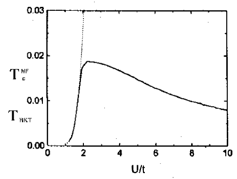
5.3 The effects of Coulomb repulsion and quantum phase fluctuations
In this section we will discuss the influence of Coulomb repulsion and quantum phase fluctuations on the phase diagram built in the previous section. We will follow the papers of Ariosa et al. [118, 119, 120, 121]. Since the discussion of the pairing mechanism is beyond the scope of the current review, we will not consider any effects directly related to the pairing mechanism suggested in [121].
5.3.1 Derivation of the quantum -model
Our starting point is the Hamiltonian [120] which describes charge carriers on a lattice, subject to an on-site attraction and a long-range Coulomb repulsion, , acting between particles on different sites:
| (5.53) |
where . Here, as before, (see Hamiltonian (3.47)) () are creation (annihilation) operators, denotes denotes pairs of nearest-neighbour sites, is the neutralizing background charge which is of course equal to the carrier density per lattice site, and .
The partition function can be written as a functional integral by means of two successive Stratonovich-Hubbard transformations [225] (see also [149, 226] and compare with Sec. 3.1.1), decoupling the two interaction terms in with the help of a complex field and a real field both of which depend on the site and the imaginary time :
| (5.54) | |||||
with a part linear in the Hubbard-Stratonovich fields
| (5.55) |
and a part containing quadratic terms
| (5.56) |
As in the earlier sections denotes a complex pairing field which couples to the local pair operator while the second real field represents a local electric potential which acts on the local charge density fluctuations . One evaluates the trace over the electronic degrees of freedom, with the definition :
| (5.57) |
Then expanding the “free energy” to fourth order in , to second order in and to leading terms in the space and time gradients of the two fields one arrives at:
| (5.58) |
where gives the result for the free electron contribution and
| (5.59) |
Here the Ginzburg-Landau coefficients , , and are related to the free electron particle-particle propagator [53, 149, 208, 172, 220, 225] and are thus temperature dependent in general; is the screened Coulomb potential (approximated by its static limit) with being the electronic polarizability.
The terms containing the Ginzburg-Landau coefficients , , and give the usual time-dependent Ginzburg-Landau free energy292929Note that the coefficient is related to the kinetic term which is not obvious from the discrete form (5.59)., which is usually supposed to be valid only very close to the transition temperature equal to or in our case. Thus these coefficients are derived in the same approximation as the phase stiffness (5.27) for the BCS limit. This, of course, does not allow one to investigate the equation equivalent to the self-consistent equation (5.28) in the regime (see the discussion in Sec. 5.2). However, the advantage of the representation (5.59) is its relative simplicity which allows one to integrate out the dependence on the electric potential . Commenting further on Eq. (5.59) note that its third term describes the coupling between the two space- and time-fluctuating Hubbard-Stratonovich fields; the fifth term in the above equation takes into account the coupling between the local electric potential and the number density fluctuations of the charge carriers, while the last double-sum is the contribution of the screened Coulomb potential to the thermodynamical potential.
Integrating over the electric potential yields
| (5.60) | |||||
where represents the number density fluctuations in the presence of the fluctuating pairing field at site . Roughly speaking, if one interprets as the wave-function of a local pair at site and, thus, its squared modulus as a “pair-density”, we note that is composed of two separate contributions, namely one from the “unpaired” charge carriers (“normal” channel) and one from the “paired” fermions (“superfluid” channel), respectively. Obviously, the charge neutrality constraint imposes .
Next the amplitude and phase of was introduced in [120] in a way similar to that discussed in the previous section. In the following discussion, relatively strong coupling was assumed [120] so that the fermions bind into on-site singlet pairs at a temperature of the order of the mean field transition temperature , well above the superconducting phase transition, the latter being finally triggered by the onset of phase order. Below , , so that the average amplitude has a non-vanishing mean value given by . Charge neutrality implies and, for [53, 149, 208, 172, 220, 225]:
| (5.61) |
Note that, as explained above, the expressions for , and the relationship between , and are, strictly speaking, valid in the vicinity of while one needs to use them well below this temperature. This is the reason why in [120] the proposal was made to use these expressions together with the zero temperature expression for taken from [117] (see Eq. (5.50) and the strong-coupling limit below). Splitting the number of pairs at a given site into , the integration over was performed in [120] which (neglecting gradient terms) yields a free energy functional for phase fluctuations only:
| (5.62) | |||||
with the phase stiffness [225, 117] .303030It may also be called Josephson coupling due to the close analogy to the quantum analysis of the Josephson junction, see the review [227] and Refs. therein. This analogy is widely used in [118, 119, 120, 226] for physical interpretation. Note that since the value of was expressed via the zero temperature gap and neglects the gradient terms for , the treatment of the classical part of the phase fluctuations becomes equivalent to that in the previous section. The interaction matrix in (5.62) is given by
| (5.65) |
The expansion of in powers of has yielded a spurious on-site repulsion between pairs. However, due to the exclusion principle, two pairs cannot sit on the same lattice site. Thus, in the following, is excluded in the last term of (5.62); this is equivalent to the usual introduction of hardcore bosons.
The final step in the derivation in [120, 226] is a standard Legendre transformation from the ”phase velocities” to the conjugate momenta , that are interpreted as the number density fluctuations of charge carriers, at site and imaginary time . The partition function that emerges from the latter transformation is equal to the one that would have been obtained from the following Hamiltonian:
| (5.66) | |||||
The Eq. (5.66) is the central result of the present section: the partition function of the Hubbard model with local attraction and long-range Coulomb repulsion has been written as a functional integral with a generalized action (or thermodynamical potential) involving a fluctuating pairing field and a local electric potential . After functional integration over the latter Hubbard-Stratonovich field and over fluctuations in , the final form of the generalized action involves:
an effective phase coupling term between the local spatial variations of the phases of , which presents the same analytical structure as the Josephson coupling term appearing in the Hamiltonian of the classical -model;
a “kinetic energy” term, representing the screened Coulomb interaction between local fluctuations of the number density of charge carriers. The Hamiltonian (5.66) represents a non-local (extended) version of so-called 2D quantum -model which, in addition to the usual Josephson coupling term, involves a non-local kinetic energy term; in the case of underdamped Josephson junction arrays, the latter describes capacitive (quantum) effects which may arise between the superconducting islands themselves but not between the superconducting islands and the normal substrate.
5.3.2 Mapping to the quantum -model with local kinetic energy. Phase diagram
Here, following [120, 121, 226] we discuss the application of the Hamiltonian (5.66) for calculating the transition temperature of strongly anisotropic superconductors, such as superlattices and bulk systems in the underdoped regime. To do this the following approximations are made:
is restricted to one superconducting layer;
the screened Coulomb interaction, which takes into account the electric coupling between layers, is modelled by an analytical form, which is similar to the usual Yukawa potential:
| (5.67) |
where is the dielectric constant of the interlayer material, is the lattice constant and is Thomas-Fermi screening length depending on the density of charge carriers according to the well-known formula
| (5.68) |
In the last expression is the Bohr radius and is a sphere diameter, related to the density of charge carriers .
considering only , the ”background shift”, , in the first term of (5.66) is neglected.
At this point one can make a connection to another, simpler model [118, 119] (which is rather similar to that proposed by Doniach and Inui [66]), based on the quantum phase fluctuation of the -model, in which the BKT transition temperature, is identified with the superconducting critical temperature in the absence of charging effects and in which is depressed from its classical value by charging (quantum) effects [228] (see also [221]). The basic Hamiltonian for this system is the quantum -model with local kinetic energy:
| (5.69) |
where is equivalent to the number of “2e-charges” which are present at site , is the self-capacitance of the site. A fundamental property of the quantum -model with a local capacitive term, is provided by the fact that and are canonically conjugate variables and therefore satisfy the following commutation relation (we restored temporarily the Planck constant in this relation):
| (5.70) |
Thus, the fluctuations of these two are intimately related. In the approach that has been used in [118, 119, 66], the relation between and real superconducting temperature, which we denote as , is given by (again we restore the Boltzmann constant ):
| (5.71) |
where is the average effective self-capacitance and is the ratio between charging and Josephson energy. Thus, within the approach [118, 119], one only has to evaluate the appropriate . It is obvious that the quantum phase fluctuations decrease with respect to evaluated in the presence of the classical phase fluctuations only : is an upper bound to the actual transition temperature [25].
It is also important to mention the results of [205] where for the quasi-2D version of the Hamiltonian (5.69) it was shown that phase fluctuations produce a linear increase in the penetration depth with increasing at low temperatures. This in turn implies a linear decrease of the full superfluid density (see the discussion in Sec. 5.4.3).
In order to apply the framework sketched above one must map the Hamiltonian (5.66) onto a “local capacitance” Hamiltonian (5.69) using the following approximation:
| (5.72) |
where
| (5.73) |
In Ref. [118] the critical temperature for the Hamiltonian density (5.69) has been evaluated in the “self-consistent harmonic approximation” (SCHA) which gives results for in good agreement with Monte Carlo simulations. A good overall fit of the numerical SCHA result is (see Refs. in [120])
| (5.74) |
When approaches =6.2, goes to zero.
One has now derived an effective Hamiltonian of the form (5.69), where the capacitance is given by Eq. (5.73), and is the phase stiffness, which is in fact temperature dependent. As seen earlier, this temperature dependence is particularly important in the high-density limit where and thus . In [121] the temperature dependence is approximated by a simple linear form chosen precisely such that i.e.
| (5.75) |
where is the zero-temperature phase stiffness. Given this fit to the phase stiffness, one can then calculate the critical temperature for the classical phase fluctuations as a function of doping. This is nothing but the BKT transition temperature, , given by Eq. (5.52) with the value of taken from Monte-Carlo simulations. The critical temperature for the quantum fluctuations (i.e. including charging effects) can then also be calculated as a function of doping using Eq. (5.74). Note that, it follows from the form of the equations, that both and are bounded above by . The phase diagram based on only the classical phase fluctuations is shown in Fig. 20.
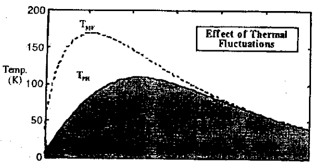
This version of the phase diagram is in fact very similar to the phase diagram presented in Fig. 15 except for details related to the pairing mechanism in Ref. [121] which results in a non-monotonic behaviour for . The idea that, in the above context, the so-called pseudogap be identified with the standard mean field superconducting gap is also proposed [121]. Nonetheless, these gaps should not be identical due to the quantum corrections, as is the case for the temperatures and or from [135] (see the discussion in Sec. 5.1.3).
The phase diagram where the effect of the quantum phase fluctuations is taken into account is shown in Fig. 21.
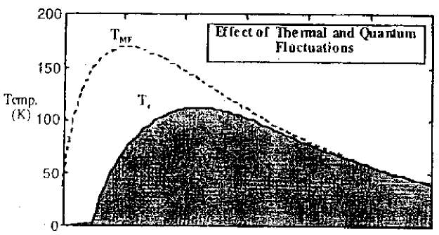
The most important effect of these fluctuations is that they push the critical temperature to zero in the underdoped region. Thus one can see that the quantum fluctuations lead to a greater overlap between the experimental phase diagram in Fig. 1 and its theoretical version in Fig. 21.
Furthermore, a possible mechanism which also pushes to zero for the overdoped region was suggested in [121]. Its discussion is however beyond the phase fluctuation scenario of this review. Finally, to make a connection with the next section, we note that another reason why is zero for overdoped systems is the presence of impurities which can also destroy superconductivity.
5.4 The effect of non-magnetic impurities
Up till this point we have considered models for the crossover and the pseudogap behaviour which do not take into account the effect of impurities. However, a discussion of the effect of impurities seems to be crucial for any realistic model of the HTSC. Indeed, it is known, that the itinerant holes in HTSC are created by doping which in turn introduces a considerable disorder into the system, for instance, from the random fields of chaotically distributed charged impurities [229]. Thus the purpose of this section is to study the influence of non-magnetic impurities on superconducting properties including the superfluid density.
In the theory of “common metals” the Fermi energy and the mean transport quasi-particle time are independent quantities which are always assumed to satisfy the criterion . In HTSC which are “bad metals” [26] both and are dependent on the doping and the abovementioned criterion may fail [229]. In particular it has been shown [229], that for strongly disordered metallic systems, superconductivity is absent if the scattering-to-pairing ratio exceeds a critical value. Secondly, for such systems [229], even if this ratio is not exceeded, superconductivity only exists for a finite range of doping.
We shall study two cases here. The first is the case of weak disorder originally studied in the papers of Anderson [230] and Abrikosov-Gor’kov (AG) [231] (see also [152]). when the superconducting order is preexisting and the criterion is satisfied. In this case superconductivity in disordered thin films was first considered by Ramakrishnan [213] using an approach very similar to the method presented in the review. The second case is that of strong disorder where this criterion is not satisfied, and superconductivity is destroyed by sufficient disorder.
We concentrate on several important aspects. The first is the influence of impurities on the phase diagram particularly at high-densities where the Fermi surface is well-developed. The second is the behaviour of superfluid density. Its temperature dependence at low () and high () temperatures is not yet understood and presents a challenge for competing theories. One of the consequences of the presence of impurities is that the value of the zero temperature superfluid density can be less than the total density of carriers, so that their presence may help to explain the experimental results for these quantities, [25, 26]. The third is the creation of inhomogeneities and the ultimate destruction of superconductivity by strong disorder.
It is interesting to note an alternative explanation for the lowered zero temperature superfluid density as a result of quantum phase fluctuations has been recently presented [232] (see also [68]). In the previous section the importance of the contribution from the quantum phase fluctuations is clearly evident. It follows that the lowering of the superfluid density is the result of at least two factors – namely impurities and quantum phase fluctuations.
5.4.1 Weak disorder limit
Anderson’s theorem [230] (see also [148]) states that in 3D the BCS critical temperature is unchanged in the presence of weak disorder in the form of non-magnetic impurities. As discussed in Sec. 5.1, the BCS critical temperature (in 2D) is the temperature at which the pseudogap opens and is unchanged by the presence of impurities. On the other hand the superconducting transition temperature is the temperature of the BKT transition. In contrast to the former, the latter (as seen in Sec. 5.1) is defined in terms of the bare superfluid density or the phase stiffness (given by the delocalized carriers) which decreases with an increasing concentration of impurities. Thus in 2D the temperature of the superconducting transition, decreases with increasing impurity concentration.
Thus, in the model with impurities, the relative size of the pseudogap phase, could be larger in the presence of impurities [114] than in the clean limit [115] and might therefore be observed over a wider range of densities.
Model and main equations
Our starting point is, as in Secs. 3.1 and 5.1, a continuum version of the 2D attractive Hubbard model defined by the simplest Hamiltonian (3.1) in the presence of impurities [152]
| (5.76) | |||||
where as before denotes the space and imaginary time variables, is a fermion field with spin , is the effective fermion mass, is the chemical potential, is an effective local attraction constant, and is the static potential of randomly distributed impurities.
From the Hamiltonian (5.76), following the derivation given in Sec. 5.1.1, one can again derive the effective Hamiltonian of the classical -model (5.14) with the bare (i.e. unrenormalized by the phase fluctuations, but including pair breaking thermal fluctuations) superfluid stiffness:
| (5.77) | |||||
Here
| (5.78) |
with
| (5.79) |
is the AG [152] Green’s function of neutral fermions averaged over a random distribution of impurities and written in the Nambu representation [233, 148]. In writing (5.77) we assumed that . This approximation, as shown by AG [152], does not change the final result for . Note also that the Green’s function (5.78) is valid only when which demands the presence of a well developed Fermi surface, which in turn implies that . Thus one cannot use the expression (5.78) in the Bose limit with .
Substituting (5.78) into (5.77), and using the inequalities to extend the limits of integration to infinity, one arrives at
| (5.80) |
Eq. (5.80) is formally divergent and demands special care due to the fact that one, in contrast to Sec. 5.1.1, has to perform the integration over before the summation [152]. Finally one can formally cancel the divergence [152] to obtain
| (5.81) |
The temperature of the BKT transition for the Hamiltonian (5.14) is determined by the self-consistent equation (5.28).
The self-consistent calculation of as a function of the carrier density as before requires additional equations for and , which together with (5.28) form a complete set (see Sec. 5.1.1).
When the modulus of the order parameter is treated in the mean field approximation, the equation for (compare with (5.29)) takes in the presence of impurities the following form
| (5.82) |
which formally coincides with the gap equation of the BCS theory. This coincidence confirms Anderson’s theorem [230] which states that in this limit the dependence of is the same as that for the clean superconductor and is not affected by the presence of non-magnetic impurities.
We recall, however, that there is both physical and mathematical differences between the gap in the BCS theory and (see Sec. 5.1 above). The main point, which we would like to stress here, is that due to the Anderson theorem [230] the value of does not depend on the presence of impurities at least when , while the temperature , as we will see below, is really lowered.
The effect of weak disorder on the pseudogap region
In the clean limit the transport time is infinite, so that
| (5.84) |
Near one can obtain from (5.84) its asymptotical form (5.27) which has been re-derived here using the reverse order for the summation and integration.
As has been explained in Sec. 5.1.2, if one inserts the dependence of given by (5.36) into (5.27) and then substitutes (5.27) into (5.28) one obtains the asymptotic expression (5.37) for the BKT temperature in the clean limit for high carrier densities.
In the high density limit one can also use the following solution of Eq. (5.34) for
| (5.85) |
(Compare Eq. (5.85) with (3.27) which reproduce together the standard BCS ratio .)
It is obvious from (5.37) and (5.85) that for a clean system the pseudogap region shrinks rapidly for high carrier densities. It is therefore natural to ask (see, for example, [107, 222] and the discussion in Sec. 5.1.2) whether precursor superconducting phase fluctuations can explain the pseudogap anomalies which are observed over a wide range of temperatures and carrier densities, since in the clean limit the relative size of the pseudogap region is, for instance, less than when the dimensionless ratio . If one makes a crude estimate for the dimensionless ratio for optimally doped cuprates one obtains - [146] which indicates that in the clean superconductor the pseudogap region produced by the phase fluctuations is too small. Of course, all these estimations are rather qualitative due to the simplicity of the model.
We now turn to the dirty limit where the transport time is small (). This inequality is not in contradiction with the weak disorder limit but merely implies high density i.e. that . In this limit one can neglect the radical in the bracket of (5.81) [152]. The remaining series is easily summed and one obtains the following expression for the bare superfluid stiffness,
| (5.86) |
As in the clean limit, due to Anderson’s theorem, the expressions (5.36) for and (5.85) for remain unchanged in the presence of impurities. Again substituting (5.36) into (5.86) one obtains
| (5.87) |
One can see that the size of the pseudogap region is now controlled by the new parameter which is an unknown function of for HTSC. If one assumes that one indeed has weak disorder i.e. clearly the pseudogap region remains small. If one however moves away from the weak disorder lint and uses values for extracted from experiment [4, 6], for which then Eq. (5.87) one does obtain an increase in the pseudogap region with impurities. Such an estimate is of necessity only qualitative.
Certainly impurities which are always present in HTSC do increase the size of the pseudogap region in the weak disorder limit. The effect however appears to be small in this limit and it seems likely that the effect of quantum phase fluctuations [232] is more important in allowing one to reproduce the experimentally observed extent of the pseudogap region. It would however be interesting to readdress this problem in the case of strong disorder.
The difference in the temperature scales for pairing and phase coherence for higher densities where is vital to the debate, previously mentioned in Sec. 2.2, as to how the approaches of Uemura [84] and Emery-Kivelson [25, 26] (see in particular [234]) are related. While Uemura [84] considers that the approach based on the phase fluctuations as “essentially identical to the BEC-BCS crossover picture”, Emery and Kivelson [234] insist that the separation of the temperature scales for pairing and phase coherence is a consequence of the fact that HTSC are doped insulators. Here we would like to present a point of view which is closer to that expressed in [234]. Indeed, as we saw in the previous chapters the indication that one is on the BEC side of the BEC-BCS is a negative sign for the chemical potential . In Sec. 5.1.2 we saw that in the region with a large pseudogap was indeed mostly negative phase, so that the statement of Uemura [84] applies. However, as we discussed optimally doped cuprates correspond to higher carrier densities where is already positive and . The presence of quantum phase fluctuations, and to a lesser extent impurities, however permits one to have a relatively big pseudogap region even on the BCS side of the crossover. Another argument in favour of the picture presented by Emery and Kivelson is that the value [32] is almost independent of doping while it increases on the BEC side of crossover, see Sec. 5.1.2. Thus the BEC-BCS crossover and the present approach based on the phase fluctuations need not be related.
We stress however that this argument about the sign of the chemical potential is not valid in the presence of spatial inhomogeneities (see discussion in Sec. 3.1.5) as for example seen in the stripe picture of Emery, Kivelson and Zachar [23]. This implies that BEC-BCS crossover and phase fluctuation picture are not mutually exclusive since for a spatially inhomogeneous system it is possible to have local regions with so small a carrier density that pre-formed Bose pairs do exist there, while in average the whole system is still on the BCS side of the crossover. This is, in some sense, similar to the many-band model considered in Sec. 3.2 where coexisting local and Cooper pairs were separated not in real, but in momentum space.
The superfluid density
In this section we contrast the experimental results for the bare and full superfluid densities with those for the clean superconductor and indicate the likely role played by impurities.
The bare superfluid density is straightforwardly expressed via the bare phase stiffness, . In particular in the clean limit, it follows from (5.84) (or (5.26) with (5.30)) that . This is not surprising since must be equal to the full density for any superfluid ground state in a translationally invariant system [235] and the clean system is translationally invariant. We note, however, as stated above that in HTSC [26]. Substituting (5.36) into (5.27) one obtains for close to the bare superfluid density
| (5.88) |
This behaviour of the bare superfluid density is formally the same as the behaviour of the full superfluid density in the BCS theory. Nevertheless it is important to remember that the full superfluid density in the present model undergoes the Nelson-Kosterlitz jump at and is zero for .
We note that one can experimentally probe both the bare superfluid density in high-frequency measurements [67] and the full superfluid density in low-frequency measurements [236]. The former describes mainly the local condensate density distribution which is, of course, nonzero above in the precursor superconductivity theories, while the latter corresponds to an average condensate density and is zero above .
A direct comparison with experiment reveals further discrepancies between experiment and the predictions given above for the clean limit. The experimental shape of the bare superfluid density (see Fig. 22 taken from [67]) disagrees with that given by Eq. (5.88).
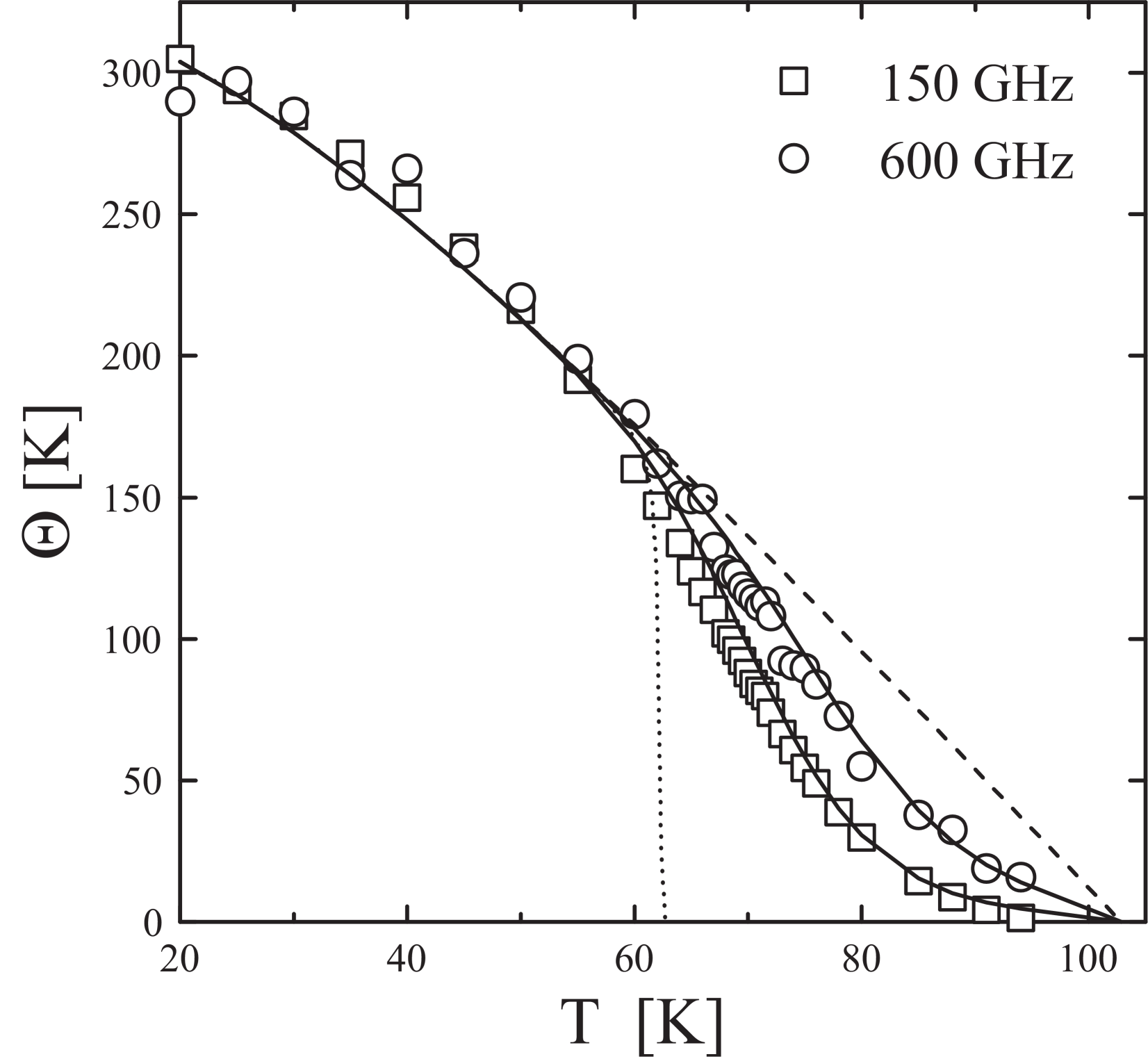
Moreover, one of the most striking features is that although remains nonzero well above , it does not persist throughout the pseudogap temperature regime. Instead it falls linearly to zero at a temperature well below . Even though the presence of impurities leads one closer to the experimentally observed behaviour of in the region (see [114]), the superfluid density still becomes zero only at . Thus the observed behaviour of the bare superfluid density at finite temperature has not yet been fully explained in this approach and presents an open question to the current theories of phase fluctuations (for another problem related to the superfluid density in the theories based on phase fluctuations see also the end of Sec. 5.4.3).
On the other hand, the zero value of above may be well understood within other scenarios which claim that pseudogap is not the result of the superconducting fluctuations but is related, for example, to charge- and/or spin-density waves as discussed in [16, 34]. In such a case there is still a superconducting contribution to the pseudogap even in the region . Since is less than , one can speculate that it could be much easier to explain the observed size of the superconducting pseudogap region even within a simple model from Sec. 5.1. Further experimental studies of the doping dependence of and its clear resolution from and are necessary.
The experimental data of [236] also shows that the full superfluid density, , does not display the Nelson-Kosterlitz jump. This is probably related to the influence of the interlayer coupling as discussed in [27].
One can however directly obtain a reduced value of the zero temperature bare superfluid density in the dirty limit. In this limit the value of the zero temperature superfluid density is given by since . This does not contradict the results of [235] because the system is not translationally invariant in the presence of impurities.
We conclude that the low value of the superfluid density in HTSC [26] may at least in part (for other mechanisms, for example, based on the quantum phase fluctuations, see [232, 68]) be straightforwardly related to the impurities which are inevitably present in HTSC. On the other hand its temperature dependence remains an important unsolved problem.
5.4.2 Strong disorder
As seen in Sec. (5.4.1) impurities are vital for an understanding of the superconducting properties of HTSC. We now turn to a discussion of these properties in the complementary case of strong disorder. In the presence of strong disorder Anderson’s theorem no longer holds, and the pairing amplitude need no longer be constant in space but is in fact spatially dependent i.e. . An analysis of this effect on the superconducting properties of -wave superconductors has been presented in [237] and we simply represent the main results here.
Model and main equations
The model is the attractive Hubbard model (see Eq. (3.47)) but with an additional site dependent disorder potential with values chosen randomly from the uniform distribution where controls the strength of the disorder
| (5.89) |
Firstly one treats the spatial fluctuations of the modulus of the order parameter in the mean field approach, using the standard Bogolyubov-de Gennes (BdG) equations [238]
| (5.90) |
where the site-dependent modulus is given by
| (5.91) |
and similarly for . Here as appropriate to a square lattice and incorporates a site-dependent Hartree shift dependent on the local number density,
The chemical potential, , is simply given by fixing the average number density, .
| (5.92) |
where is the number of sites. These equations are non-linear and have to be solved self-consistently for the BdG eigenvalues and the eigenvectors . In practice they are solved numerically on a finite lattice with periodic boundary conditions.
Single-particle spectral gap and bare superfluid stiffness
Several random realizations for the disorder are considered. For each realization one solves the BdG equations to find and then averages over the disorder to obtain a probability distribution for the local pairing amplitudes. For weak disorder, , is strongly peaked at its mean-field (BCS) value and one thus recovers a spatially uniform . The distribution broadens significantly for and is rather skewed for with a large weight near .
One can then also construct the disorder averaged one-particle density of states from the BdG eigenvalues
| (5.93) |
and this has been plotted in [237] for three different disorder strengths . The most important feature of these plots is the fact that there is a finite spectral gap even at high disorder. For each individual representation of the disorder, the lowest eigenvalue , remains non-zero and of the order of the zero disorder BCS gap and this is the origin of the spectral gap. This occurs despite the fact that, for high disorder, a large fraction of the sites have near zero pairing amplitudes.
There is however a particularly simple explanation for this behaviour in the high disorder limit as follows. Plotting one observes superconducting “islands”, (i.e. clusters of sites where is large) which correspond to regions where is small. These are surrounded by a larger “sea” of sites with and where is large. The lower lying BdG eigenvalues correspond to the superconducting islands and so have finite gap. The BdG eigenvalues corresponding to the “sea” have even higher energies because the corresponding disorder potential is large.
One notes that in this procedure [237] one calculates the spectrum and for each individual disorder representation and then disorder averages. This will clearly give different results from the procedure [239] of constructing a disorder averaged and then looking at the energy gap. In the latter case one smoothes out the amplitude fluctuations and, in contrast to the picture presented here, one obtains a gap which closes with increasing disorder [239]. Note that it is not possible to prove that the single-particle strength at is exactly zero (particularly for weak coupling ) since the numerical calculations are by necessity in a finite system. Furthermore, note that the gap will be filled by the presence of phase fluctuations, as in the case of zero disorder which will be discussed in Chap. 7.
One can also calculate the bare superfluid stiffness, , given by [240]
| (5.94) |
The diamagnetic term is one-half (in 2D) the kinetic energy and the paramagnetic term is the (disorder averaged) transverse current-current correlation function. From Fig. (23) one can see a reduction in of two orders of magnitude with increasing disorder. It never however becomes zero showing that superconductivity is not destroyed by amplitude fluctuations.

In the strong disorder limit regardless of the dimensionless coupling . It is thus vital to consider phase fluctuations and preliminary calculations in [237] show that it is these fluctuations which are responsible for the destruction of superconductivity at high disorder.
5.4.3 Discussion
Since in HTSC the pairing scale is different from the superconducting transition temperature the role of non-magnetic impurities is not traditional and they in fact define the superconducting properties of a “bad metal”. In particular even for weak disorder we have seen that these impurities strongly depress the superfluid density at zero temperature bringing it closer to that experimentally observed. In the case of strong disorder, impurities lead to large inhomogeneities in the system with the existence of isolated superconducting islands. This effect then dramatically changes the superconducting properties, as evidenced by a greatly reduced bare superfluid stiffness, and ultimately leads to the destruction of superconductivity.
Of course, the results presented are only qualitative since only the simplest model with non-retarded -wave attraction and an isotropic fermion spectrum was considered. However, there are some indications that for -wave pairing, the properties obtained will persist [241].313131Note that -wave superconductivity appears to be completely destroyed by relatively weak disorder if one describes the system within the AG theory used in Sec. 5.4.1. However, it is shown in [241] using the finite temperature version of the BdG equations (5.90) for -pairing, that -wave superconductivity may well survive even for strong disorder. This difference results from the more adequate treatment of the spatial fluctuations of the complex ordering field modulus in [241]. One also notes that -wave superconductivity can be stable in the strong coupling limit, or on the BEC side of the BCS-BEC crossover [242].
Further studies of the superfluid density are necessary. For example, it is important to explain the concentration dependence of the full superfluid slope, at [236, 17].323232It appears to be more difficult to understand why as in the weak coupling model. However, as mentioned in the beginning of Sec. 3.1 it is the doped carriers that are weakly coupled and in fact a half-filled band in the strong coupling model corresponds here to the empty conduction band. As already mentioned in Sec. 5.3.2 the classical phase fluctuations333333While the quantum -model was considered in [205] for more exact quantitative estimates, it was shown in this paper (see also more recent publication [27]) that the linear slope of the low temperature full superfluid density is produced by the classical phase fluctuations. result in the linear slope of the full superfluid density. Nevertheless, as shown in [243] (see also [39]) the linear dependence can be also produced by the nodal (Dirac) quasiparticles with a relativistic dispersion law which are present in a d-wave superconductor. It is now widely discussed whether the main contribution to the observed slope of the low temperature superfluid density is due to these quasiparticles (see e.g., [244, 245]) or phase fluctuations [27, 246]. It is likely that the dominant contribution to the slope varies with doping as suggested in [246]. While in the optimally- and over-doped samples it is produced by the nodal quasiparticles, in the underdoped samples it can be compatible with the model of classical phase fluctuations. We stress only at the end that the problem of the superfluid slope in HTSC should be considered also in the presence of defects of different origin (including dopants).
6 The Green’s function in modulus-phase representation and non-Fermi liquid behaviour
The main quantity of interest in the present chapter is the one-fermion Green’s function . The associated spectral function , being proportional to the intensity of the ARPES [7, 8], encodes information about the pseudogap and quasi-particles. Following [125] the Green’s function for the charged (physical) fermions is given by the convolution (in momentum space) of the propagator for neutral fermions which has a gap and the Fourier transform of the phase correlator .
Thus the approximation employed here assumes the absence of coupling between the spin and charge degrees of freedom. This can however be taken into account at the next stage of approximation. Nonetheless, as we shall see, the phase fluctuations result in non-Fermi liquid behaviour of the system both below and above the superconducting transition temperature, .
6.1 The modulus-phase representation for the fermion Green function
The starting point is a continuum version of the two-dimensional attractive Hubbard model (3.1). As discussed in Sec. 3.1.1 the model with the Hamiltonian density (3.1) is equivalent to a model with an auxiliary BCS-like pairing field. This equivalent model has a Hamiltonian density, which is given in terms of the Nambu variables and (see Eq. (3.2)) and the auxiliary complex Hubbard-Stratonovich fields and , as
| (6.1) |
Let us consider the full fermion Green’s function in the Matsubara finite temperature formalism
| (6.2) |
The frequency-momentum representation for (6.2) in the case of the BCS theory in 3D (i.e. in the mean field approximation) is given by (3.15).
However, a problem arises when one tries to apply Eq. (3.15) directly to 2D systems at , since a non-zero value for is forbidden by the CMWH theorem [126] (see also the discussion in Secs. 2.3). Nevertheless as was discussed in Sec. 5.1 one can assume that the modulus of the order parameter has a nonzero value, while its phase defined by (5.3) is a random quantity. To be consistent with (5.3) in Sec. 5.1 the spin-charge variables (5.4), which separate the Nambu spinors into their modulus and phase, were simultaneously introduced.
Applying (5.4) the Green’s function (3.15) can be split into spin and charge parts
| (6.3) |
where
| (6.4) |
is the Green’s function for neutral fermions. We note here that this equation implies that there is no interaction between the spin and charge degrees of freedom. Introducing the projectors one gets
| (6.5) |
so that Eq. (6.3) may be rewritten as
| (6.6) |
where and correspond to the diagonal and non-diagonal parts of the Green’s function respectively.
There is good reason to believe (see Sec. 5.1) that, for close to , fluctuations of the modulus of the order parameter343434These are so-called longitudinal fluctuations which correspond to fluctuations of the carrier density and undoubtedly must be taken into account in the very underdoped region. are irrelevant. Thus one may safely use for the Green’s function (6.8) of the neutral fermions the mean-field approximation given by Eq. (5.17) (compare with (3.15)).
As we shall see, fluctuations of the -phase transform the pole in the Green’s function for the neutral fermions (5.17) into a branch cut in the Green’s function for the charged particles (6.2) for . The CMWH theorem [126] concerning the absence of spontaneous breaking of a continuous symmetry in 2D means that symmetry-violating Green’s functions which are described by terms with nonzero and must vanish. However, it says nothing about the gap in the spectrum of excitations, as is sometimes incorrectly stated. The correct explanation is that if the symmetry is unbroken, and the fermion excitation appears as a pole in the two-point function (6.2), then the fermion must be gapless. If the fermion does not have the same quantum numbers as (e.g. the neutral fermion ) and so does not appear in the two-point function (6.2) as a one-particle state, then symmetry does not tell us whether the fermion () will be gapless or not. Thus there is no contradiction between the gapped form (5.17) and the CMWH theorem. We note that this formal consideration [210] closely resembles the more physical arguments presented by Abrikosov [64] about the possible existence of a gap in the one-particle excitation spectrum without the presence of long-range order.
6.2 The correlation function for the phase fluctuations
As stated above, phase fluctuations are expected to be responsible for the differences between the properties of the charged (physical) and the neutral fermions defined above. The latter are described by the Green’s function (5.17) which coincides with the BCS Green’s function (3.15)) only if one assumes that the phase of the order parameter is a constant and can be chosen to be zero. This is not the case in the 2D model, where there is a decay of phase correlations and the Green’s functions of charged and neutral fermions are non-trivially related via Eq. (6.7). To establish their relationship one needs to know the correlator for phase fluctuations. Its calculation is quite straightforward for , while for one may apply the results of the theory of the BKT transition (see e.g. [133] or the other textbooks mentioned).
6.2.1 The correlator for
In the superconducting phase free vortex excitations are absent and the exponent correlator is easily expressed in terms of the Green’s function
| (6.10) |
(here as above ) via the Gaussian functional integral
| (6.11) | |||
where the source is given by
| (6.12) |
The Green’s function
| (6.13) |
for the phase fluctuations has already been found in Sec. 5.1.1 and follows directly from Eq. (5.25). Recall that the superfluid stiffness (see Eq. (5.26)) and the compressibility (see Eq. (5.22)) are both functions of , and , and also that the Green’s function (6.13) includes only the lowest order derivatives of the phase . Higher terms are also present in the expansion, but will be neglected.
Substituting (6.13) into (6.2.1) one gets
| (6.14) |
It is easy to see that for zero frequency the integral in Eq. (6.14) is divergent at unless . Thus in the sums over in Eq. (6.7) only two terms survive, namely
| (6.15) |
It is important that terms like which are proportional to and thus violate the gauge symmetry, do not contribute in Eq. (6.7) due to vanishing of the and correlators which follow them. This explicitly demonstrates that the non-diagonal part of the 2D Green’s function is equal to zero at all finite temperatures353535Strictly speaking, one can state this, based on Eq. (6.14), only for . However, there are relatively simple arguments [247] why a correlator of the form must be identically zero both below and above . Indeed, we know that the correlator (see Eq. 6.23 below) tends to zero as . On the other hand according to the principle of weakening correlations our correlator must reduce to the product at large , i.e.the vacuum expectation value must be identically zero. This of course simply means that one is in the symmetric phase, i.e. one has an exact symmetry with respect to the transformation . In turn this means that all correlators which violate this symmetry are identically zero. in accordance with the CMWH theorem.
For the non-zero correlators one has
| (6.16) | |||||
In the following discussion only the static case will be considered. The restriction to this case is one of the few main assumptions used throughout this chapter. Recall also another essential assumption made in this chapter which is the absence of coupling between the spin and charge degrees of freedom.
The summation over and the integration over in (6.16) can readily be done yielding the following expression for the argument of the exponent in (6.16)
| (6.17) |
where we have introduced the scale
| (6.18) |
which is a function of the variables used (in the simplest case ).
In (6.17) we introduced a cutoff by hand with the introduction of the corresponding exponential function. This cutoff represents the maximal possible momentum in the theory – the Brillouin momentum.
One can derive from (6.17) (see the details in [125]) the following asymptotic results
| (6.19) |
This long-distance behaviour then governs the -fluctuations physics to be studied below.
Let us discuss the meaning of the value . Using again the phase stiffness and compressibility from Eqs. (5.26) and (5.22) one readily gets that – the single-particle thermal de Broglie wavelength ( is the Fermi energy). Then, considering that and taking as given by (see Sec. 5.1.2), one can estimate
| (6.20) |
The value of the Fermi momentum for cuprates is less than the Brillouin momentum . Thus the first line of (6.19) appears to be more relevant.
There is a second way to estimate . One can rewrite it in terms of the value of in the form
| (6.21) |
where is the BCS coherence length. (It is assumed, that for the carrier densities of interest, , so that the coherence length and the pair size are the same. See Sec. 3.1.5). This shows that has the meaning of a coherence length, which appears to be rather natural since the minimal size of the region where there is the phase coherence should be of the order of . Since the coherence length in cuprates is larger than the lattice space , one again obtains that the first line of (6.19) should be applied. Therefore for and for static fluctuations we have that
| (6.22) |
where . Note that all these estimations are correct for the clean system. For the dirty system one should replace them by the results from Sec. 5.4.
6.2.2 The correlator for
For the expression for the static correlator (6.22) can be generalized using well-known results from the theory of the BKT transition as [130, 131, 133]:
| (6.23) |
where
| (6.24) |
is the BKT coherence length and the value of to be used in numerical calculations will be discussed later.
Note that Eq. (6.24) represents a very specific temperature dependence of the coherence length which is completely different from the temperature dependence of the Ginzburg-Landau coherence length. The charge and spin susceptibilities for the negative- Hubbard model (3.47) were estimated in [248] using the BKT and Ginzburg-Landau coherence lengths. It appears that the spin susceptibility calculated with the BKT coherence length better fits the Monte Carlo data. The fact that the BKT coherence length, with its specific temperature dependence, is used allows one to go beyond the -matrix approximation, and to adequately describe the physics of the topological BKT superconducting fluctuations.
There is also an analogy between the renormalized classical regime discovered in [135], when below the temperature (see Sec. 4.5) the two-particle correlation length grows exponentially, and the exponential growth of the BKT coherence length below .
One may consider Eq. (6.23) as a general representation for both for and if the coherence length is considered to be infinite for . The pre-exponential factor in Eq. (6.23) is related to the longitudinal (spin-wave) phase fluctuations, while the exponent is responsible for the transverse (vortex) excitations, which are present only above . The pre-exponential factor appears to be important for the presence of non-Fermi liquid behaviour which we discuss below. Note, however, that the longitudinal phase fluctuations could be suppressed by the Coulomb interaction [123] which is not included in the present simple model. One further comment is that while the approximation used in [123] to study the vortex fluctuations is good for well above , the form of the correlator here is appropriate for close to .
The constant may be estimated from the condition that cannot be much less than the parameter which appears in the theory as a natural cutoff, so we will use in our numerical calculations . In any case, for where the expression (6.24) is valid, the value is large and not as sensitive to the initial value of .
There is also a dynamical generalization of (6.23)
| (6.25) |
proposed in [122] from a phenomenological background. Note that is the real time and is here the decay constant, so that (6.25) is the retarded Green’s function. The temperature dependence of for the case of a classical 2D planar magnet was studied in [249] and showed a critical slowing down as due to the disappearance of mobile, free vortices.
The more general case of the dynamical phase fluctuations (6.25) was considered in a related calculation [122] (see its discussion in Sec. 7.3) where a correlator 363636It differs from the correlator (6.25) only by a factor multiplying the phase., which includes dynamical phase fluctuations, has been used in the numerical calculation of the self-energy of the fermions and the subsequent extraction of the spectral function from the fermion Green’s function.
6.3 The Fourier transform of
For the Fourier transform (6.9) of (6.23) one has
| (6.26) | |||||
The integral in (6.26) can be calculated (see, for example, [250]) leading to
| (6.27) |
The hypergeometric function in (6.27) may be well approximated by a constant since it is slowly varying at all values of . As such a constant we can take the value of hypergeometric function at . Thus,
| (6.28) |
where
| (6.29) |
It should be stressed that for the parameter quickly deviates from unity as decreases; in other words, the underdoped region will reveal more non-standard properties than the overdoped one.
One should take into account that even for the propagator (6.28) does not have the canonical behaviour which is typical, for example, for the Bogolyubov mode in dimensions . In 2D, modes with a propagator , would lead to severe infrared singularities [126], and to avoid this, the modes transform into the softer ones (, ).
Finally, substituting (6.15) and (6.28) into (6.7) one obtains
| (6.30) |
The coincidence of the Matsubara frequency in the left and right sides of Eq. (6.30) is straightforwardly related to the static approximation. It is truly remarkable that the Green’s function (6.30) may be evaluated exactly, as may the expressions for the spectral density and for the density of states. We note, however, that the static approximation can be justified only a posteriory when the dynamical case is also considered [260].
6.4 The derivation of the fermion Green’s function in Matsubara representation and its analytical continuation
The calculation of the fermion Green’s function can proceed analytically along the same lines of calculation as in the relativistic case of the Gross-Neveu model at [247] One splits the fermion part of (6.30) in the following manner
| (6.31) |
where
| (6.32) |
Then , using the representations
| (6.33) |
and
| (6.34) |
and taking into account (6.31), one may rewrite (6.30) as
| (6.35) | |||||
Note that the special form of the integral representation (6.33) (compare with the representation (6.34)) guarantees that the Gaussian integral over is well-defined independently of the sign of . Now the Gaussian integration over momenta in (6.35) can be done explicitly. Subsequently changing the variables and then one can integrate over . Finally, making the substitution and expanding the quadratic polynomial in the denominator, gives (see the details in [125]):
| (6.36) | |||||
where
| (6.37) |
with
| (6.38) |
and
| (6.39) |
One can check from (6.37) that for , so that one can rotate the integration contour to the real axis:
| (6.40) |
Then the integral representation (6.40) may be analytically continued to . The change of variable allows Eq.(6.40) to be expressed in terms of Appell’s function [251]
| (6.41) |
so that
| (6.42) | |||||
For the BKT coherence length is infinite () so that the first argument of the Appell’s function . This allows one to apply the reduction formula [251]
| (6.43) |
and express the result via the hypergeometric function
| (6.44) | |||||
where the value of from (6.29) has been substituted.
6.4.1 The retarded fermion Green’s function
To obtain the expression for spectral density, one firstly needs to obtain the retarded real-time Green’s function from the temperature Green’s function. One does this by means of the analytical continuation , so that . This results in the following rules (compare with (6.32), (6.37), (6.38))
| (6.45) |
| (6.46) |
with
| (6.47) |
and
| (6.48) |
Thus for the retarded Green’s function one has
| (6.49) | |||||
It is also easy to see that
| (6.50) |
Let us now discuss the conditions under which the imaginary part of is nonzero.
For one can see that, , so that is real and . The case is more complicated. It follows from the Appell’s function transformation property [251]
| (6.51) |
that for real and the function becomes complex if or/and . This implies that has an imaginary part if or/and . Looking at the expressions (6.46) for and one can see that is always positive, while may be negative. This means that has an imaginary part if . Now using (6.50) the condition for existence of nonzero imaginary part of can be written in the following form .
6.5 The branch cut structure of and non-Fermi liquid behaviour
Let us consider firstly the retarded fermion Green’s function (6.44) for . Applying the rules for analytical continuation from the previous subsection to Eq. (6.44) one gets
| (6.52) | |||||
Near the quasi-particle peaks when the arguments of the hypergeometric function in (6.52) are close to 1. One can consider, for instance, the first hypergeometric function, so that
| (6.53) |
Using the following relation between the hypergeometric functions [251]
| (6.54) |
one gets that near
| (6.55) |
It is evident that the expression obtained for the Green’s function is non-standard. In addition to containing a branch cut, it clearly displays its non-pole character. The latter in its turn corresponds to the non-Fermi liquid behaviour of the system as a whole. It must be underlined that the non-Fermi liquid peculiarities are strictly related to the charged (i.e. observable) fermions only – the Green’s function (5.17) of the neutral ones has a typical (pole type) BCS form. It also follows from (6.55) that the new properties appear as a consequence of the -particle presence (leading to ), and because the parameter is a function of (see (6.29)) non-Fermi liquid behaviour increases with increasing temperature and is preserved until vanishes.
It is interesting that, in Anderson’s theory [252, 253] (see also [59]), it was postulated that Fermi liquid theory breaks down in the normal state as a result of strong correlations. To introduce this breakdown the following form of the single-particle fermion propagator for the normal state was assumed (see e.g. [253, 254]):
| (6.56) |
where is a frequency cutoff which is introduced to make the Green’s function dimensionally correct, is independent of and is some function of (see more detail in [254] where this form of Green’s function was used as the starting point for the evaluation of the pair fluctuation propagator and the electronic self-energy). It follows from (6.56) that the associated spectral function satisfies close to the Fermi surface a non-Fermi liquid homogeneity relation:
| (6.57) |
where the limiting case of a Fermi liquid has .
Here we started from Fermi liquid theory and found that it has broken down due to strong phase fluctuations, so that the final equation (6.55) reveals the same analytical structure as (6.56). The non-Fermi liquid behaviour may, as suggested in [252, 59], lead to the suppression of coherent tunnelling between layers, that in turn confines carriers in the layers and leads to strong phase fluctuations. However, in contrast to [252, 253, 254], the present model predicts the restoration of Fermi liquid behaviour as decreases, since when .
The limit can be also obtained in the following way. Strictly speaking one cannot estimate the value of in the limit in (6.52) via Eq. (6.20) because the substitution of the relationship into (6.18) is not valid in this case. However, this is not essential because so that the correlator (6.22), which clearly establishes long-range order in the system. Furthermore, the value of in (6.29) goes to 1 for so that the hypergeometric function in (6.52) directly reduces to the geometrical series:
| (6.58) |
Therefore, substituting (6.58) into (6.52) one gets for the diagonal component of the Nambu-Gor’kov Green’s function the ordinary BCS expression
| (6.59) |
Clearly Eq. (6.59) results in the standard BCS spectral density [49] with two -function peaks
| (6.60) |
To recover the non-diagonal components of one has to restore the correlators and that were omitted in Sec. 6.2.1.
7 The spectral function in the modulus-phase representation and filling of the gap
As is well known, [49, 148, 152, 184], the spectral features of any system are entirely controlled by its spectral density. In terms of the matrix Greens’ function (6.49) this is given by
| (7.1) |
and, for example, in the cuprates is measured in ARPES experiments [4, 7, 8, 9] (see also [10], where a transparent example shows how interaction, finite experimental resolution and other effects destroy a simple function-like spectral function). The spectral function defines the spectrum anisotropy, the presence of a gap, the DOS, etc. Thus it is important to discuss its behaviour for the different models based on phase fluctuations.
7.1 Absence of gap filling for the Green’s function calculated for the static phase fluctuations in the absence of spin-charge coupling
In this section we discuss for the Green’s function obtained above in Sec. 6. This example is rather instructive since it allows one to obtain an analytical expression for the spectral function [125], check the sum rule and explicitly show the limitations of the static, non-interacting approximation used to calculate the Green’s function and its spectral density.
7.1.1 An analytical expression for the spectral density
For and the retarded fermion Green’s function (6.49) can be rewritten (see Appendix B) in the following form
| (7.2) | |||||
Then, according to (7.1) the spectral density for the Green’s function (7.2) has the form:
| (7.3) |
Using the quadratic transformation for the hypergeometric function [251]
| (7.4) |
the expression (6.29) for , Eqs. (6.46) and (6.47) one finally obtains
| (7.5) | |||||
where the chemical potential can be, in principle, determined from the equation (5.30) which fixes the carrier density. Here, however as stated above, one assumes that the carrier density is sufficiently high that .
7.1.2 The sum rule for the spectral density
It is well-known that for the exact Green’s function the spectral function (7.1) must satisfy the sum rule
| (7.6) |
The Green’s function (6.49) calculated here is, of course, approximate. One reason for this is the use of the long-distance asymptotic result (6.19) for the phase correlator (6.16). This means that its Fourier transformation (6.28) is, strictly speaking, valid for small only, while the expressions have been integrated out to infinity. Another approximation that has been made is the restriction to static phase fluctuations. Thus it is important to check whether the sum rule (7.6) is satisfied with sufficient accuracy.
It is remarkable that for (7.5) the sum rule (7.6) can be tested analytically (see the details in [125]). One can derive the following result,
| (7.7) |
The numerical value of the integral at the temperatures of interest may be estimated in the following way. At the phase stiffness is given by , so that for near to the value from (6.29) is
| (7.8) |
In particular, yields the following estimate for the right hand side of (7.7), . This shows that for the spectral density (7.5) is reasonably good.
The parameter can however differ strongly from unity at and in the underdoped regime.
7.1.3 Main results for the spectral density. The problem of gap filling. Limitations of numerical analytical continuation

To draw these plots the value of from Eq. (7.8) and the mean-field value of obtained from Eq. (5.33) were used.
The temperature dependence of the spectral function (7.5) is discussed in detail in [125]. It is shown, in particular, that below the quasi-particle peaks at have a finite temperature dependent width which is, of course, related to the spin-wave (longitudinal) phase fluctuations. When the width goes to zero, but this limit cannot be correctly derived from (7.5) because this is an ordinary function, while the BCS spectral density (6.60) is a distribution. This sharpening of the peaks with decreasing in the superconducting state was experimentally observed [8] and represents a striking difference from the BCS “pile-up” (6.60) which is present for all .
It was pointed out in [123] (see Sec. 7.2) that the broadening of the spectral function caused by these fluctuations can be greater than the experimental data permits.
For the quasi-particle peaks become less pronounced as the temperature increases. Indeed, the value of at is, in contrast to the case , already finite. This is caused by the fact that since is now finite due to the influence of vortex fluctuations. As the temperature increases further, decreases so that the quasi-particle peaks disappear (see Fig. 24). This behaviour qualitatively reproduces the ARPES studies of the cuprates for the anti-node direction [8] (see also [9]) which show that the quasi-particle spectral function broadens dramatically when passing from the superconducting to normal state.
It is important to stress that due to the very smooth dependence of on (see Eq. (6.24)) as the temperature varies from to there is no sharp transition at the point . In particular, there is a smooth evolution of the superconducting (excitation) gap into the gap which is also equal to and in fact can be called a pseudogap because at the system is not superconducting. This qualitatively fits experiment [4, 8, 9, 31] and appears to be completely different from BCS theory [49], where the gap vanishes at .
We, however, would like to stress the main reason why further studies are essential. While the temperature behaviour of the quasi-particle peaks is quite similar to experiment [4, 8], the gap in the spectrum remains unfilled, i.e. the spectral density is identically zero inside the gap ( for ). Furthermore, there is also an excess of the spectral weight on the gap edges which is seen as the extra peaks [125]. This is obviously related to the facts that the classical phase fluctuations were treated in the static approximation and that the coupling between the spin and charge degrees of freedom was neglected. One therefore needs to consider how these effects could lead to the filling of the gap.
The -matrix approximation seems to result in the opposite result. For example, the classical fluctuations do lead to a pseudogap, as shown by the Hubbard model at half-filling [135]. We note, however, that our statement is applicable to the uncoupled static phase fluctuations only and neglects entirely modulus fluctuations. Further studies are necessary to make a comparison of this analytical result for the phase fluctuations with other complementary approaches, which we believe should reproduce our result when the same assumptions are made. Here we make only one further comment related to the numerical analytical continuation.
It is very instructive to estimate the accuracy one would expect if a similar problem were to be investigated numerically. Using the analytical expression (6.42) obtained for the Green’s function on the imaginary axis one can perform its numerical analytical continuation by means of Padé approximants [194] (see also [183] and a recent comprehensive discussion of the method in [195]). Using Eq. (6.42) calculated to ten digits of precision we tried to recover the known spectral function (7.5) shown in Fig. 24, but even for 110 Matsubara frequencies the numerical result presented in Fig. 25 cannot indicate whether the gap is filled or not.

As already mentioned in Sec. 4.1, numerical analytical continuation is often used for the subsequent extraction of the spectral function in the methods where the -matrix equations are solved numerically on the imaginary axis. It is clear, however, that the precision of the numerical solution is even less than that used above for Eq. (6.42) and thus numerical results alone are insufficient for definitive conclusions about pseudogap filling. There is however a real-time technique [99, 100, 104] which allows one to avoid numerical analytical continuation, but demands some other assumptions.
The results discussed in this section show that, while the physical picture based on non-interacting static phase fluctuations is sufficient to derive at least the qualitative phase diagram, additional consideration is necessary to understand the mechanisms responsible for gap filling. Thus the next two sections will be devoted to two possible ways that the pseudogap can be filled.
7.2 Gap filling by static phase fluctuations due to quasi-particle vortex interactions. The phenomenology of ARPES
As shown by Franz and Millis [123] (see also [124]) one way of filling the gap can be obtained for static phase fluctuations via the coupling of the spin and charge degrees of freedom which leads to a Doppler shift for the quasi-particles.
As already discussed in Sec. 6.2, for this mechanism the disordered state above can be thought of as a “soup” of fluctuating vortices with positive and negative topological charges and with total vorticity constrained to zero. Each of these vortices is surrounded by a circulating supercurrent which decays as with the distance from the core. Such supercurrents, within a semiclassical approximation, lead to a Doppler-shifted local quasi-particle excitation spectrum of the form [238, 255]
| (7.9) |
where is the local superfluid velocity and is the usual BCS spectrum. The change in the local excitation spectrum will affect the spectral properties of the superconductor in that the physically relevant spectral function must be averaged over the positions of fluctuating vortices.
This effect will be particularly pronounced in a -wave superconductor since Eq. (7.9) implies the formation of a region around a nodal point on the Fermi surface with for arbitrarily small . Physically this corresponds to a region of gapless excitations on the Fermi surface which leads to a finite density of states (DOS) at the Fermi level. As first discussed by Volovik [256], a similar situation arises in the mixed state of a -wave superconductor where the superflow around the field-induced vortices leads to a residual DOS proportional to .
7.2.1 Phenomenological and phase fluctuation coupled Green’s functions
In the mean field approximation (neglecting, among other things, phase fluctuations) the diagonal Green’s function was written in [123] (compare with Eq. (5.17))
| (7.10) |
where the angular dependence of the gap function for -wave superconductor is and following [257] the single particle scattering rate was added to the usual mean-field solution to describe the ARPES data in the overdoped samples where there are no strong pseudogap effects. It is instructive to use Dyson’s equation (4.3) to extract from (7.10) the expression for self-energy as done in [257, 9]
| (7.11) |
Note that the form of the scattering rate in () constitutes a non-trivial assumption. It is not pair-breaking, in the sense that it is ineffective at small and ; i.e. in the region . By contrast in a -wave superconductor, a conventional scattering rate enters via the replacement , leading to a broadening which is effective even at low and . As shown by Norman et al. [257] the form given in Eqs. (7.10) and (7.11) agrees with the ARPES data at . It is demonstrated in [123] that it also agrees with STS.
At Norman et al. [257] showed that additional pair-breaking scattering is needed to account for the ARPES data in the underdoped case where the gap is filled well above , They modelled this phenomenologically by introducing another scattering rate , and making the replacement in the last term of Eqs. (7.10) and (7.11):
| (7.12) |
They suggested that could arise from exchange of pair fluctuations and precisely this kind of effect has been intensively studied within -matrix approximation (see Sec. 4.1), but as argued in [123, 135] this proposed mechanism does not account for the observed magnitude of .
As mentioned above another likely source of the pair-breaking scattering leading to gap filling has been suggested in [123], namely supercurrents induced by phase fluctuations. In order to determine how is changed in the presence of superflow it is useful to recall the origin of the energy shift in Eq. (7.9). This can be derived [238, 255] by assuming a state of uniform superflow with induced by an order parameter of the form . By solving the appropriate set of Bogolyubov-de Gennes equations and retaining only terms to linear order in , one finds that the energy is modified as indicated in (7.9) while the coherence factors are to the same order unchanged. This result is then semiclassically extended to non-uniform situations by assuming slow spatial variations of .
One can follow this exact procedure and solve the appropriate Gor’kov equations for in the presence of superflow. One finds the following intuitively plausible result which is exact for uniform flow up to terms linear in :
| (7.13) |
where . Here is the Fermi velocity and the last equality holds when the Fermi surface is approximately isotropic. In the following it is assumed that Eq. (7.13) can be applied locally when varies slowly in space. Applying the above prescription to (7.10) one finds, again to the leading order in ,
| (7.14) |
where with . One can easily estimate which is typically a small number in superconductor. One therefore expects that . A more detailed numerical analysis indeed shows that, as long as is small compared to unity, the effect of on the spectral lineshape is negligible compared to that of , and will be dropped in the following.
A typical experimentally measured quantity, such as the ARPES or STS lineshape, will provide information on the spectral function associated with averaged over the phase fluctuations (see also [258]). Thus, one needs to evaluate
| (7.15) |
where is the probability distribution of given by
| (7.16) |
The angular brackets indicate thermodynamic averaging over the phase fluctuations in the ensemble specified by the 2D Hamiltonian (5.14).
Further details of the precise derivation and the comparison with the ARPES and STS experimental data can be found in [123], but will not be discussed here since our main goal is simply to discuss possible mechanisms for gap filling. We note only that since the calculations reported in [123], new and controversial ARPES data has been obtained [10, 11].
As already discussed the last term in Eq. (7.10) can be thought of as a superconducting self-energy given by Eq. (7.11). Eqs. (7.14) and (7.15) then imply that the primary effect of the phase fluctuations is to smear the functional dependence of on the energy variable, broadening the spectral lineshape. The detailed analysis performed in [123] shows that acts primarily to fill in the gap, in a way similar to the inverse pair lifetime introduced by phenomenological considerations in Ref.[257]. , on the other hand, does not affect the lineshape at low energies: notice that since the self-energy given by Eq. (7.11) diverges at the point , if , the corresponding Green’s function for any .
7.2.2 Discussion
The qualitative behaviour of ARPES and STS lineshapes (see [4, 8, 31, 257]) in underdoped BiSCCO clearly establishes the existence of a scattering mechanism which becomes operative at and which acts primarily to fill in the gap at low energies.
It is shown by Franz and Millis [123] that vortex phase fluctuations associated with proliferation of unbound vortex-antivortex pairs in the system interacting with the quasi-particles provide a reasonable explanation for this scattering.
Analysis of [123] also indicates that longitudinal (spin wave) phase fluctuations are almost completely suppressed, above and below . As we mentioned in Sec. 5.3.2 (see also Sec. 5.4.3) it has been proposed in [205] that in high- materials, longitudinal phase fluctuations governed by the Hamiltonian (5.14) are important in that they significantly contribute to the observed temperature dependence of the magnetic penetration depth. The broadening of the spectral function which would be caused by these fluctuations was calculated in [123], and it was found that it is much greater than the experimental data would permit. They therefore conclude that longitudinal fluctuations are suppressed, perhaps by the Coulomb interaction.
Quantitatively there exists considerable discrepancy between the parameters describing the ARPES and STS lineshapes, in particular the single particle scattering rate . It is possible that this discrepancy can be resolved using new ARPES data [10, 11].
Sizable transverse phase fluctuations implied by this work will also affect other properties of the underdoped systems, such as the electronic specific heat, fluctuation diamagnetism and transport [258]. Vortices existing above should also generate local magnetic fields which are zero on average but have a non vanishing variance. If such fields could be detected, e.g. by muon spin rotation experiment, this would constitute direct evidence for the phase fluctuation model of the pseudogap phase.
7.3 Gap filling due to dynamical phase fluctuations without quasi-particle vortex interactions
Another mechanism of the pseudogap filling due to vortex-vortex dynamics has been suggested by Capezzali and Beck [122] where the same -wave pairing model as in Sec. 6 was considered. This model is treated by the Stratonovich-Hubbard transformation (see Sec. 3.1.1), decoupling the interaction term by the complex pairing field . The one-electron Green’s function is then approximately given by [97, 226]:
| (7.17) |
The expression for the self-energy in the next to leading order approximation
| (7.18) |
involves the dynamic correlation function of the pairing field. Note that Eq. (7.18) does not contain the leading order of the self-energy which is included into the Green’s function (7.17) via the term with pairing field (compare with Eqs. (7.11) and (7.12)). In diagrammatic language Eq. (7.18) corresponds to a two-vertex bubble, one of the lines of which represents the propagator of the complex bosonic Hubbard-Stratonovich field, while the other line corresponds to the dressed propagator of the fermions.
In [122] rather than aiming at a self-consistent solution as described in Sec. 4, a simple form for the pairing correlation function was assumed and its influence on the one-electron properties were investigated. Introducing the amplitude and phase in the pairing field (see Eq. (5.3)) but without the corresponding replacement for the Fermi field (see Eq. (5.4), Capezzali and Beck made the following assumptions:
The mean-field transition temperature is, following [32], identified with the temperature . Below this temperature the amplitude (modulus) fluctuations are assumed to be space- and time-independent, i.e. they are treated in the mean-field approximation in a way similar to that discussed in Secs. 5.1 and 6.1. They are thus approximated by a typical mean-field (BCS-like) analytical form (see Eq. (5.36)),
| (7.19) |
where is treated as a free parameter. For BCS theory it is given by . Note that once more the average is zero. Using the definition of the Fourier transform (3.13), and space and time independence of the amplitude, one can obtain that
| (7.20) |
The Fourier transform of the phase correlator in (7.20) was taken in the form given by Eq. (6.25) (see the details in Sec. 6.2, in particular the last paragraph of the section). Thus the main difference between the first assumption of [122] and the assumptions used in Chap. 6 is the consideration of the more general case of the dynamical phase fluctuations. As will soon become apparent it is their presence that leads to gap filling.
Below the critical temperature one keeps the same form (6.25) for the phase correlations, but with , corresponding to the algebraic decay of correlations. However, in contrast to the calculations in Chap. 6, a non-zero coupling between the planes (in the third dimension) is taken into account in [122]. This is achieved by introducing a non-zero value for the average of , with a variable parameter . Due to the presence of the third direction the nonzero value of is not forbidden by the CMWH [126] theorem.
7.3.1 Discussion
For numerical computation the value of from (7.18) was evaluated in [122, 226] to lowest order by using the noninteracting with an isotropic spectrum .
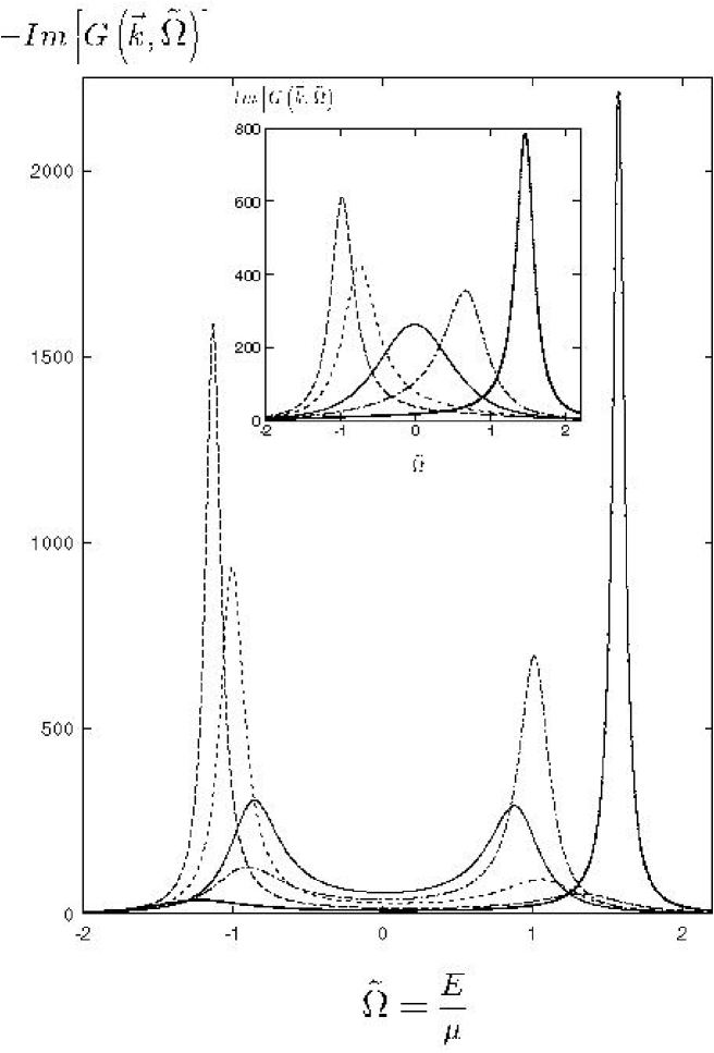
In Fig. 26 we show the spectral function from [122] obtained for the decay constant (see Eq. 6.25) and the modulus strength (see Eq. 7.19) . The following observations can be made on the basis of this figure and the other results presented in [122] :
Above , a pseudogap opens around . Its effective width is almost -independent, in spite of the -dependence of in the self-energy.
Below , but well above , one sees a one-peak structure in the spectral function for all wave-vectors , centered below (above) the chemical potential for . As one approaches , a two peak structure emerges for wavevectors where the peak below (above) the chemical potential has a greater spectral weight for . This structure becomes increasingly visible near where the density of states at the chemical potential, , becomes practically zero for all . Thus in this limit the pseudogap is delimited by two rather pronounced peaks.
It is important that, in contrast to the previous section, the filling is achieved without any vortex-quasi-particle interactions. This, of course, does not exclude the fact that there are phase fluctuations. If one could divide the total contribution of the fluctuations in (7.20) into the classical () and other (in some sense non-classical with ) fluctuations, it can be shown that the latter contribution also results in some gap filling [260].
Below , the presence of produces two new peaks: a true ”superconducting gap” emerges out of the pseudogap. Its width is given by the geometrical superposition of average and fluctuating part of . The fluctuations of the latter remain visible in the form of secondary shoulders inside the superconducting gap which approach each other about in the same proportion as the main peaks move away from each other.
The value for the decay constant is relatively large. For a smaller , and in particular for the case of critical slowing down of phase fluctuations () [249] the two shoulders would become secondary peaks inside the superconducting gap.
Near , as seen above, the spectral functions are doubly peaked in some wave-vector domain around . In this case the width of the pseudogap is given by the separation between these two peaks, which is essentially determined by . At higher temperatures, approaching , the spectral functions have only one peak. However their width is enhanced over essentially the same -domain. Due to this fact, the pseudogap fills up gradually, as is approached (from below), but with little change in its width.
Thus the mechanism for gap filling due to vortex-vortex interactions which are described by dynamical phase fluctuations can be also regarded as a strong candidate. Both mechanisms are based on the same physical premise, namely the existence of a “soup” of vortices above . Indeed both mechanisms ought to be present simultaneously, but it is not yet clear which is the dominant mechanism for gap filling, and more studies are certainly needed.
On the other hand, it must be pointed out that the existence of fluctuating vortices is not a necessary condition for the appearance of a pseudogap. Indeed, systems with symmetry (where is the number of the order parameter components) do not have topologically stable vortices, but still may possess a pseudogap-like regime. As discussed in [261] there is a situation when the second order phase transition in such a system is driven by long-wavelength transverse (or directional in terms of [261]) fluctuations, and not by longitudinal (or size) fluctuations as happens in more conventional scenarios. During this sort of transition the ordering field acquires firstly as the temperature decreases its size (modulus) while the direction is still strongly fluctuating and only a further temperature decrease leads to the formation of the ordered state. Thus one can concede this scenario of a second order phase transition leaves room for pseudogap-like behaviour even in more general theories where the stable vortex excitations are absent. Nevertheless, their presence in the particular case of theory considered here suggests that vortices can play an essential role and their specific contribution may even be dominant in this case.
8 Concluding remarks
We have concluded the description of the physical properties of 2D metals in which conductivity is the result of doping. We paid particular attention to the normal and superconducting properties directly related to phase fluctuations of the complex ordering field which increase significantly as the carrier density decreases. The vital role of phase fluctuations for phase transitions in low dimensional systems, as mentioned above, has been clearly outlined in the classical papers of Berezinskii, Kosterlitz and Thouless and the many other physicists who followed. However for many years physicists have ignored the important fact that even above (), in the so called normal phase, there is a remaining non-zero parameter, which drastically changes the spectrum of the phase and leads to pseudogap behaviour. While in theoretical papers this feature was simply overlooked, experimental techniques probably did not have sufficient precision to observe the pseudogap. During the last 3-5 years the situation has drastically changed and the resolution of ARPES and thermodynamical experiments permit one to measure quite subtle spectral features, and thus leading to the discovery of the pseudogap. According to Abrikosov “the pseudogap in the quasi-particle spectrum above and its amazing stability in strongly underdoped samples was the most spectacular among phenomena” observed in high- compounds [64]. The theory discussed above, however, does not relate the pseudogap appearance directly to the superconducting properties of oxides and stresses the possible main role of the low dimensionality of their magnetic and electron spectra. And indeed, the experimental data is not in contradiction with this conclusion. Pseudogap features have already been found in quasi-1D superconductors [262, 263] as well as in the HTSC systems mentioned above. It is interesting that pseudogap behaviour close to the Fermi level is also seen in 3D manganite systems [264]. However, in the last case its connection with some kind of fluctuation is under question [265]. Nevertheless even if the pseudogap in manganites is caused by different effects, it is remarkable, that in all these cases the systems are bad metals, i.e. for the systems under consideration, the undoped state is an insulator and conductivity only results from doping.
Throughout this review we discussed mainly the simplest 2D fermi-system with attraction. There is, however, a general theoretical question as to what are the generic effects that lead to a pseudogap. It is clear that to gain greater insight into this problem a wider class of the models should be considered. Nevertheless, some general arguments can be given already. First of all, the lowered dimensionality of the space is an essential component. This results in the CMWH theorem that allows one to state that there is a new region between the mean-field transition temperature and a true transition temperature which is in for the systems with two-component () order parameter may be well approximated by the of topological transition temperature, . This case of symmetry, which is relevant for superfluids and superconductors, led us to the rich BKT physics of vortices that undoubtedly contributes to the pseudogap properties of these systems. However, as we saw even in these 2D systems the pseudogap region appears to be small if the carrier density is too high, or in other words the coherence length is too big and size fluctuations dominate over directional [261]. In this coherence length should be even smaller [261] and therefore the conditions for the pseudogap in 3D is difficult if not impossible to satisfy.
What would happen if one considers a multi-component () order parameter? Since there is no stable vortices in this case, the topological transition is also absent. Thus as mentioned, for example, in [112] the higher symmetry of the order parameter space leads to an even larger region with directional fluctuations than in the case of symmetry. Therefore the larger dimensionality of the space of the order parameter also favours pseudogap formation. Further study of these types of models would be helpful for a deeper understanding of the pseudogap origin.
A series of experiments, in particular, NMR, neutron scattering and spin relaxation demand the introduction of the concept of a spin gap. This is not surprising because the undoped magnetic subsystems, which are antiferromagnetic insulators have spins localized on the copper ions and are characterized by the magnetic anisotropy of “easy plane” type. This shows that the average magnetic moment of every site is nonzero, and therefore the average antiferromagnetic vector in the basic CuO2 plane is also nonzero.373737It is remarkable that in the paper [266] the role of these planes in the physics of HTSC is compared with the role of the hydrogen atom in atomic physics. Doping which suppresses the long-range magnetic order, does not, however, suppress the average value of the modulus of the spin on the lattice point. This spin can also be parametrized via its modulus and phase. Then the physical picture in the spin spectrum will be very similar to that for superconductivity, when the gap in the spectrum is related to the average spin (modulus of the magnetisation) and the absence of the long-range order is the result of “disorder” by angular (directional) fluctuations which can also be described by a correlation function. Thus the system may have an additional crossover temperature related to modulus formation for another – spin – physical value. The consideration of this system, which will be close to that described above, is given either by the 2D sigma model or by the model of nearly antiferromagnetic liquid. We did not however describe them in detail because our goal was to present simple analytical (but at the same time, we hope, non-trivial) models which can lead to pseudogap character in the one-particle spectrum. The spin aspect inevitably demands in the absence of long-range order a separate treatment and the explanation is therefore less clear, and was avoided for simplicity.
Another important and new feature we wanted to stress is the role of impurities. All bad metals are such that each carrier has its “own” dopant. Thus it is necessary to show that impurities do not lead to pseudogap suppression. It is clear, however, that this direction needs substantial development to include more fully the physically relevant case of strong disorder and the effects of localization. As seen above, these effects are probably in fact responsible for the development of an inhomogeneous state.
Finally, it is very important to develop the theory for the case of anisotropic pairing. Although, as we saw, the BCS-Bose crossover theory has already been generalized to the case of -wave pairing, the formation of an anisotropic pseudogap and an anisotropic BKT transition remain serious problems to be addressed.383838Here we refer a reader to a very recent paper [267] which exploits a discrete version of the variable transformation (5.3), (5.4) to study the low temperature properties even for -wave pairing. Unfortunately, the analytical treatment of the problem is very limited and, as we saw in Sec. 7.1.3, numerical methods have their own limitations.
Therefore, there is no doubt that physicists studying pseudogap properties have many problems to solve and the results described above are only one step in this process.
Appendix A Calculation of the effective potential
Here we sketch the derivation of the effective potential. To obtain it one must write Eq. (5.12) in the momentum representation:
| (A.1) |
where
| (A.2) |
are the inverse Green’s functions. Note that the derivation of the effective potential (3.16) in the “old” and variables differs only in the replacement of the term by .
The exponential factor is added to (A.1) (see also Eqs. (3.63), (4.6), (4.11), (4.21) and (5.83)) to provide the correct regularization which is necessary to perform the calculation with the Green’s functions [152]. For instance, one obtains
| (A.3) |
where
and
To calculate the sum in (A.3), one must first use the identity , so that (A.1) takes the form
| (A.4) | |||||
Calculating the determinants of the Green’s functions (A.2) one obtains
| (A.5) | |||||
where the role of in the regularization of is now evident . The summation in (A.5) can be done if one uses the representation
| (A.6) |
and then
| (A.7) |
We find
| (A.8) |
Integrating (A.8) over , one thus obtains
| (A.9) |
Finally, substituting (A.9) into (A.5),
| (A.10) |
It is easy to show that at , the expression (A.10) reduces to that obtained in Sec. 3.1.2.
Finally, we give formulas for the summation over the Matsubara frequencies used in Secs. 5.1.1:
| (A.11) | |||||
Appendix B Another representation for the retarded Green’s function
Here we shall obtain another representation for the retarded fermion Green’s function which is more convenient for the derivation of the spectral density. Recall that when the imaginary part of is nonzero and , . This allows one to transform the analytically continued (by means of Eq. (6.46)) integral
| (B.1) |
from Eq. (6.42) in the following manner ()
| (B.2) | |||||
The first Appell function in (B.2) can be reduced to the hypergeometric function using the identity [251] which is valid for
| (B.3) |
Thus one gets
| (B.4) |
This finishes the derivation of Eq. (7.2).
References
- [1] J.G. Bednorz, K.A. Müller, Possible high- superconductivity in the Ba-La-Cu-O system, Zeitschr. Phys. B 64 (1986) 189-193.
- [2] B.G. Levi, Evidence Accumulates for Unusual Behavior in Underdoped High- Superconductors, Physics Today, 49 (1996) 17-19.
- [3] B.Batlogg, C.M. Varma, The underdoped phase of the cuprate superconductors, Phys. World N. 2 (2000) 33-37.
- [4] T. Timusk, B. Statt, The pseudogap in high temperature superconductors: an experimental survey, Rep. Progr. Phys. 62 (1999) 61-122.
- [5] J. Friedel, Quasi-low-dimensionality in the weak coupling limit, Physica C 153-155 (1988) 1610-1616.
- [6] A.V. Puchkov, D.N. Basov, T. Timusk, The pseudogap state in high- superconductors: an infrared study, J. Phys. (Cond. Mat.) 8 (1996) 10049-10082.
- [7] Z.-X. Shen, D.S. Dessau, Electronic structure and photo-emission studies of late transition-metal oxides — Mott insulators and high-temperature superconductors, Phys. Rep. 253 (1995) 1-162.
- [8] M. Randeria, J.C. Campuzano, in: Proceedings of the International School of Physics, “Enrico Fermi”, Varenna, 1997 (IOS Press, Amsterdam, 1998), Preprint cond-mat/9709107.
-
[9]
M.R. Norman, H. Ding, H. Fretwell,
M. Randeria J.C. Campuzano,
Extraction of the electron self-energy from angle resolved
photo-emission data: application to Bi2212,
Phys. Rev. B 60 (1999) 7585-7590;
M.R. Norman, H. Ding, M. Randeria J.C. Campuzano, Electron self-energy of high temperature superconductors as revealed by angle resolved photo-emission, Preprint cond-mat/9710185. - [10] Y.-D. Chuang, A.D. Gromko, D.S. Dessau et al., A re-examination of the electronic structure of and – An electron like Fermi Surface and the absence of flat bands at , Int. J. of Mod. Phys.B 13 (1999) 3597-3600; Preprint cond-mat/9904050.
- [11] D.L. Feng, W.J. Zheng, K.M. Shen et al., Fermi surface of Bi2212: a systematic revisit and identification of almost perfectly nested Fermi surface segments, Preprint cond-mat/9908056.
- [12] A.J. Arko, Gaps, pseudogaps, and Occam’s razor, Science 284 (1999) 752-753.
- [13] D.A. Wollman, D.J. Van Harligen, J. Giapintzakis, D.M. Ginsberg, Evidence for pairing from the magnetic field modulation of YBaCu3O7–Pb Josephson junctions, Phys. Rev. Lett. 74 (1995) 797-800.
- [14] W.N. Hardy, D.A. Bonn, D.C. Morgan, et al., Precision measurements of the temperature dependence of in YBa2Cu3O6.95: strong evidence for nodes in the gap function, Phys. Rev. Lett. 70 (1993) 3999-4002.
- [15] D.J. Scalapino, The case for pairing in the cuprate superconductors, Phys. Rep. 250 (1995) 329-375.
- [16] R.A. Klemm, What is the symmetry of the high-T-c order parameter? Int. J. of Mod. Phys.B 12 (1998) 2920-2931.
- [17] J. Mesot, M.R. Norman, H. Ding et al., Changes in the superconducting gap anisotropy with doping and implications for the penetration depth, Phys. Rev. Lett. 83 (1999) 840-843; Preprint cond-mat/9812377.
- [18] R. Gatt, S. Christensen, B. Frazer et al., Superconducting gap vs. wave vector: Evidence for hot regions on the Fermi surface, Preprint cond-mat/9906070.
- [19] G.G.N. Angilella, A. Sudbø, R. Pucci, Extended -wave superconductivity: Flat nodes in the gap and the low-temperature asymptotic properties of high- superconductors, Preprint cond-mat/0001046, to appear in Eur. Phys. J. B.
- [20] R.A. Klemm, G. Arnold, A. Bille et al., c-axis twist Bi2SrCaCu2O8+δ Josephson junctions: A new phase-sensitive test of order parameter symmetry, Int. J. of Mod. Phys.B 13 (1999) 3449-3454.
- [21] R.B. Laughlin, Magnetic Induction of Order in High- Superconductors, Phys. Rev. Lett. 80 (1998) 5188-5191.
- [22] V.M. Loktev, Mechanisms of high-temperature superconductivity of Copper oxides, Fiz. Nizk.Temp. 22 (1996) 3-45 [Engl. trans.: Low Temp. Phys. 22 (1996) 1-32].
- [23] O. Zachar, Effect of magnetic field on overdoped HTc superconductors: Conflicting predictions of various HTc theories, Preprint cond-mat/9902130.
-
[24]
D. Pines, Spin Fluctuations and
Pairing in High-Temperature Superconductors,
Tr. J. of Physics 20 (1996) 535-547;
J. Schmalian, D. Pines, B. Stojkovic, Microscopic theory of weak pseudogap behavior in the underdoped cuprate superconductors I: General theory and quasi-particle properties, Phys. Rev. B 60 (1999) 667-686; Preprint cond-mat/9804219. - [25] V. Emery, S.A. Kivelson, Importance of phase fluctuations in superconductors with small superfluid density, Nature 374 (1995) 434-437.
- [26] V. Emery, S.A. Kivelson, Superconductivity in Bad Metals, Phys. Rev. Lett. 74 (1995) 3253-3256.
- [27] E.W. Carlson, S.A. Kivelson, V.J. Emery, E. Manousakis, Classical phase fluctuations in high temperature superconductors, Phys. Rev. Lett. 83 (1999) 613-616.
- [28] K. Gorny, O.M. Vyaselev, J.A. Martindale et al., Magnetic field independence of the spin gap in YBa2Cu3O7-δ, Phys. Rev. Lett. 82 (1999) 177-180.
- [29] G.Q. Zheng, Y. Kitaoka, K. Asayama et al., Pseudogap and superconductivity under high magnetic field in underdoped high- cuprate, Int. J. of Mod. Phys.B 13 (1999) 3764-3766.
- [30] A.V. Fedorov, T. Valla, P.D. Johnson et al., Temperature dependent photo-emission studies of optimally doped Bi2Sr2CaCu2O8, Phys. Rev. Lett. 82 (1999) 2179-2182.
- [31] Ch. Renner, B.Revaz, J.H. Genoud et al., Pseudogap precursor of the superconducting gap in under- and overdoped Bi2Sr2CaCu2O8+δ, Phys. Rev. Lett. 80 (1998) 149-152.
-
[32]
M. Oda, K. Hoya, R. Kubota et al.,
Strong pairing interactions in the underdoped
region of Bi2Sr2CaCu2O8+δ,
Physica C 281 (1997) 134-142;
T. Nakano, N. Momono, M. Oda, M. Ido, Correlation between the doping dependencies of superconducting gap magnitude and pseudogap temperature in high- cuprates, J. Phys. Soc. Jpn. 67 (1998) 2622-2625. - [33] J.L. Tallon, J.W. Loram, The doping dependence of - what is the real high- phase diagram? Preprint cond-mat/0005063.
- [34] V.M. Krasnov, A. Yurgens, D. Winkler et al., Evidence for coexistence of the superconducting gap and the pseudo-gap in Bi-2212 from intrinsic tunneling spectroscopy, Phys. Rev. Lett. 84 (2000) 5860-5863.
- [35] V.J. Emery, S.A.Kivelson, O. Zachar, Spin-gap proximity effect mechanism of high-temperature superconductivity, Phys. Rev. B 56 (1997) 6120-6147.
- [36] V.J. Emery, S.A. Kivelson, J.M. Tranquada, Stripe phases in high temperature superconductors, Proc. Natl. Acad. Sci. USA 96 (1999) 15380; Preprint cond-mat/9907228.
- [37] S. Caprara, C. Castellani, C. Di Castro et al., The stripe-phase quantum-critical-point scenario for high- superconductors, J. Phys. IV 9 (1999) 329-332; Preprint cond-mat/9812279.
- [38] S.-C. Zhang, Unified theory base on symmetry of superconductivity and antiferromagnetism, Science 275 (1997) 1089-1096.
-
[39]
P.A. Lee, X.-G. Wen, Unusual superconducting
state of underdoped cuprates,
Phys. Rev. Lett. 78 (1997) 4111-4114;
D.H. Kim, P.A. Lee, Theory of spin excitations in undoped and underdoped cuprates, Ann. Phys. 272 (1999) 130-164. - [40] T. Senthil, M.P.A. Fisher, L. Balents, C. Nayak, Quasi-particle Transport and Localization in High- Superconductors, Phys. Rev. Lett. 81 (1998) 4704-4707.
- [41] T. Senthil, J.B. Marston, and M.P.A. Fisher, Spin quantum Hall effect in unconventional superconductors, Phys. Rev. B 60 (1999) 4245-4254.
- [42] A.S. Alexandrov, A.B. Krebs, Polarons in High-temperature Superconductors, Usp. Fiz. Nauk 162 (1992) No 5, 1-85.
- [43] A.S. Alexandrov, N.F. Mott, Polarons and Bipolarons (World Scientific, Singapore, 1995).
- [44] B. Jankó, I. Kostin, K. Levin, M.R. Norman, D.J. Scalapino, Incoherent pair tunnelling as a probe of the cuprate pseudogap, Phys. Rev. Lett. 82 (1999) 4304-4307.
- [45] G. Deutscher, Coherence and single-particle excitations in high-temperature superconductors, Nature 397 (1999) 410-412.
- [46] D.E. Sheely, P.M. Goldbart, J. Schmalian, A. Yazdani, Andreev interferometry as a probe of superconducting phase correlations in the pseudogap regime of the cuprates, Preprint cond-mat/0001039.
- [47] S. Onoda, M. Imada, wave pairing fluctuations and pseudo spin gap in two-dimensional electron systems, J. Phys. Soc. Jpn. 68 (1999) 3121; Preprint cond-mat/9903030.
- [48] A. Kobayashi, A. Tsuruta, T. Matsuura, Y. Kuroda, Pseudogap induced by superconducting fluctuations in the model, J. Phys. Soc. Jpn. 68, No.8 (1999); Preprint cond-mat/9907006.
- [49] J.R. Schrieffer, Theory of Superconductivity (Benjamin, New York, 1964).
- [50] J. Polchinski, Effective Field Theory and the Fermi Surface, in: Proceedings of the 1992 TASI, eds. J. Harvey and J. Polchinski (World Scientific, Singapore, 1993), Preprint hep-th/9210046.
- [51] D. Mihailovic, B. Podobnik, J. Demsar et al., Divergence of the quasi-particle lifetime with doping and evidence for pre-formed pairs below in YBa2Cu3O7-δ: Direct measurements by femtosecond time-resolved spectroscopy, J. Phys. Chem. Solids 59 (1998) 1937.
- [52] J. Demsar, B. Podobnik, J. Evetts et al., Evidence for crossover from a Bose-Einstein condensate to a BCS-like superconductor with doping in YBa2Cu3O7-δ from quasi-particle relaxation dynamics experiments, Europhys. Lett. 45 (1999) 381-386.
- [53] M. Randeria in: Bose-Einstein Condensation, edited by A. Griffin, D.W. Snoke, and S. Stringari (Cambridge University Press, New York, 1995) p.355-392.
- [54] V.M. Loktev, S.G. Sharapov, Superconducting condensate formation in metallic systems with arbitrary carrier density, Cond. Mat. Phys. (Lviv) No 11 (1997) 131-177.
-
[55]
B. Jankó, J. Maly, K. Levin,
Pseudogap effects induced by resonant pair scattering,
Phys. Rev. B 56 (1997) 11407-11411;
Superconductivity from a pseudogapped normal state: a mode coupling approach to precursor superconductivity, Phys. Rev. B 59 (1999) 1354-1357;
Numerical studies of the -wave pseudogap state and related : the “pairing approximation” theory, Physica C 321 (1999) 113-133;
Pairing correlations and pseudo-gap state: Application of the “Pairing approximation” theory, Preprint cond-mat/9805018;
I. Kosztin, Q. Chen, B. Jankó, K. Levin, On the relationship between the pseudo- and superconducting gaps: Effect of residual pairing correlations below , Phys. Rev. B 58 (1998) R5936-5940;
Pairing fluctuation theory of superconducting properties in underdoped to overdoped cuprates, Phys. Rev. Lett. 81 (1998) 4708-4712. - [56] Q. Chen, I. Kosztin, B. Jankó, K. Levin, Superconducting transitions from pseudo-gap state: d-wave symmetry, lattice, and low dimensional effects, Phys. Rev. B 59 (1999) 7083-7094.
- [57] I. Kosztin, Q. Chen, Y.-J. Kao, K. Levin, Pair excitations, collective modes and gauge invariance in the BCS – Bose-Einstein crossover scenario, Phys. Rev. B 61 (2000) 11662-11675.
- [58] J. Demsar, B. Podobnik, V.V. Kabanov et al., The superconducting gap , the pseudogap and pair fluctuations above in overdoped Y1-xCaxBa2O7-δ from femtosecond time-domain spectroscopy, Phys. Rev. Lett. 82 (1999) 4918-4921.
- [59] P.W. Anderson, The theory of superconductivity in the High- cuprates (Princeton Univ. Press, 1997).
- [60] A.A. Tsvetkov, D. van der Marel, K.A. Moler et al., Global and local measures of the intrinsic Josephson coupling in Tl2Ba2CuO6 as a test of the interlayer tunnelling model, Nature 395 (1998) 360-362.
- [61] J.H. Choy, S.J. Kwon, G.S. Park, High- superconductors in the two-dimensional limit: [(Py-CnH2n+1)2HgI4]-Bi2Sr2Cam-1CumOy ( and 2), Science 280 (1998) 1589-1592.
- [62] V.L. Berezinskii, Destroying of Long-Range Order in One- and Two-Dimensional Systems with Continuous Group Symmetry. I. Classical Systems, Zh. Eksp. Teor. Fiz. 59 (1970) 907-920; J. Kosterlitz, D. Thouless, Ordering, Metastability and Phase Transitions in Two-Dimensional Systems, J. Phys. C6 (1973) 1181-1203.
- [63] T. Schneider, J.M. Singer, Phase transition approach to high temperature superconductivity: Universal properties of cuprate superconductors, (Imperial College Press, London 2000).
- [64] A.A. Abrikosov, Size of the BCS ratio in strongly underdoped high- cuprates, Phys. Rev. B 55 (1997) 6149-6151; Resonant tunneling in high- superconductors, Usp. Fiz. Nauk 168 (1998) 683-695.
- [65] A.K. Nguyen, A. Sudbø, Onsager loop transition and the first-order flux-line lattice melting in high- superconductors, Phys. Rev. B 57 (1998) 3123-3143.
- [66] S. Doniach, M. Inui, Long-range Coulomb interactions and the onset of superconductivity in the high- materials, Phys. Rev. B 41 (1990) 6668-6678.
- [67] J. Corson, R. Mallozi, J. Orenstein, J.N. Eckstein, I. Bozovik, Vanishing of phase coherence in underdoped Bi2Sr2CaCu2O8+δ, Nature 398 (1999) 221.
- [68] J. Corson, J. Orenstein, J.N. Eckstein, I. Bozovik, Low temperature AC conductivity of Bi2Sr2CaCu2O8+δ, Preprint cond-mat/9908368.
- [69] R.A. Ogg, Bose-Einstein condensation of trapped electron pairs. Phase separation and superconductivity of metal-ammonia solutions, Phys. Rev. 69 (1946) 243-244.
- [70] I.M. Dmitrenko, In the world of superconductivity, (Naukova Dumka, Kiev, 1981), in Russian.
- [71] A. Griffin, A Brief History of Our Understanding of BEC: From Bose to Beliaev Author: Allan Griffin Comments: Lecture given at the “BEC Varenna Summer School”, 1998. To be published in: Bose-Einstein Condensation in Atomic Gases, eds. M. Inguscio, S. Stringari and C. Wieman (Italian Physical Society, 1999), Preprint cond-mat/9901123.
-
[72]
M.R. Schafroth,
Superconductivity of a charged boson gas,
Phys. Rev. 96 (1954) 1149;
Theory of superconductivity; Phys. Rev. 96 (1954) 1442;
Superconductivity of a charged ideal Bose gas, Phys. Rev. 100 (1954) 463-475. - [73] J.M. Blatt, Theory of superconductivity, (Academic Press, New York, 1964).
- [74] H.P.R. Frederikse, J.F. Schooley, W.R. Thurber et al., Superconductivity in ceramic, mixed titanates, Phys. Rev. Lett. 16 (1966) 579-581.
-
[75]
D.M. Eagles,
Effective masses in Zr-doped superconductivity ceramic SrTiO3,
Phys. Rev. 178 (1969) 668-676;
Possible pairing without superconductivity at low carrier concentrations in bulk and thin-film, Phys. Rev. 186 (1969) 456-463. - [76] D.M. Eagles, R.J. Tainsh, C. Andrikins, Evidence for pairing without superconductivity from resistance between 130mK and 70mK in a specimen of ceramic Zr-doped SrTiO3, Physica C 157 (1989) 48-52.
- [77] A.J. Leggett in: Modern Trends in Theory of Condensed Matter, edited by A. Pekalski and R. Przystawa (Berlin, Springer-Verlag, 1980) p.13-41.
- [78] M. Marini, F. Pistolesi, G.C. Strinati, Evolution from BCS superconductivity to Bose condensation: analytic results for the crossover in three dimensions, Europ. Phys. J.B 1 (1998) 151-159.
- [79] P. Nozières, S. Schmitt-Rink, Bose-condensation in an attractive Fermion gas: from weak to strong coupling Superconductivity, J. Low Temp. Phys. 59 (1985) 195-211.
- [80] K. Miyake, Fermi Liquid Theory of Dilute Submonolayer 3He on Thin 4He II Film, Progr. Theor. Phys. 69 (1983) 1794-1797.
- [81] M. Imada, A. Fujimori. Y. Tokura, Metal-insulator transition, Rev. Mod. Phys. 70 (1998) 1039-1264.
- [82] G.S. Boebinger, Y. Ando, A. Passner et al., Insulator-to-metal crossover in the normal state of La2-xSrxCuO4 near optimum doping, Phys. Rev. Lett. 77 (1996) 5417-5420.
- [83] C.C. Almasan et al., in: Proceedings of the Second International Conference on New Theories, Discoveries, and Applications of Superconductors and Related Materials, Las Vegas, 1999, Int. J. of Mod. Phys.B 13 (1999).
-
[84]
Y.J. Uemura, L.P. Le, G.M. Luke et al.,
Basic Similarities among Cuprate, Bismuthate, Organic, Chevrel-Phase and
Heavy-Fermion Superconductors Shown by Penetration-Depth Measurements,
Phys. Rev. Lett. 66 (1991) 2665-2668;
Y.J. Uemura, A. Keren, L.P. Le et al., Magnetic-field penetration depth in K3C60 measured by muon spin relaxation, Nature 352 (1991) 605-607;
Y.J. Uemura, Bose-Einstein to BCS Crossover picture for High- Cuprates, Physica C 282 (1997) 194-197. - [85] Ch. Niedermayer, C. Bernhard, U. Binninger et al., Muon spin rotation study of the correlation between and in overdoped Tl2Ba2CuO6+δ, Phys. Rev. Lett. 71 (1993) 1764-1767.
- [86] V.L. Ginzburg. Superconductivity and superfluidity (what is done and what is not done), Usp. Fiz. Nauk 167 (1997) 429-454.
- [87] R. Mic̆nas, J. Ranniger, S. Robaszkievicz, Superconductivity in Narrow-Band Systems with Local Non-retarded Attractive Interactions, Rev. Mod. Phys. 62 (1990) 113-171.
- [88] G. Baym, Self-consistent approximations in many-body systems, Phys. Rev. 127 (1962) 1391-1401.
- [89] G. Baym, L.P. Kadanoff, Conservation laws and correlation functions, Phys. Rev. 124 (1961) 287-299.
- [90] R. Haussmann, Crossover from BCS superconductivity to Bose-Einstein condensation: a self-consistent theory, Z. Phys. B 91 (1993) 291-308.
- [91] O. Tchernyshyov, Noninteracting Cooper pairs inside a pseudogap, Phys. Rev. B 56 (1997) 3372-3380.
- [92] M.Yu. Kagan, R. Frésard, M. Capezzali, H. Beck, One-electron spectral functions of the attractive Hubbard model for intermediate coupling, Phys. Rev. B 57 (1998) 5995-6002.
-
[93]
J. Serene,
Stability of two-dimensional Fermi liquids against pair fluctuations
with large total momentum,
Phys. Rev. B 40 (1989) 10873-10877;
J. J. Deisz, D. W. Hess and J. W. Serene, Coupled electrons and pair fluctuations in two dimensions: a transition to superconductivity in a conserving approximation, Phys. Rev. Lett. 80 (1998) 373-376. - [94] R. Frésard, B. Glaser, P. Wölfle, Self-consistent -matrix approximation to the negative- Hubbard model: numerical results, J. Phys. (Cond. Mat.) 4 (1992) 8565-8572.
- [95] R. Micnas, M.H. Pedersen, S. Schafroth et al., Excitation spectrum of the attractive Hubbard model, Phys. Rev. B 52 (1995) 16223-16232.
- [96] R. Haussmann, Properties of Fermi-liquid at the Superfluid Transition in the Crossover Region between BCS Superconductivity and Bose-Einstein Condensation, Phys. Rev. B 49 (1994) 12975-12983.
- [97] M.H. Pedersen, J.J. Rodríguez-Núñez, H. Beck et al., Superconducting properties of the attractive Hubbard model, Z. Phys. B 103 (1997) 21-28.
- [98] S. Schafroth, J.J. Rodríguez-Núñez, H. Beck, Some global properties of the attractive Hubbard model in the superconducting phase: the -matrix approximation in two dimensions, J. Phys. (Cond. Mat.) 9 (1997) L111-L118.
-
[99]
M. Letz, R.J. Gooding,
A self-consistent, conserving theory of the attractive Hubbard
model in two dimensions,
J. Phys. (Cond. Mat.) 10 (1998) 6931-6951;
M. Letz, in: the proceedings of the “XXII School of Theoretical Physics”, Ustron 98, Preprint cond-mat/9905018. -
[100]
B. Kyung, E.G. Klepfish, P.E. Kornilovitch,
Density-induced breaking of pairs in the attractive Hubbard model,
Phys. Rev. Lett. 80 (1998) 3109-3112;
P.E. Kornilovitch, B. Kyung, Pseudogap and photo-emission spectra in the attractive Hubbard model, J. Phys. (Cond. Mat.) 11 (1999) 741. - [101] M. Keller, W. Metzner, U. Schollwöck, Thermodynamics of a superconductor with strongly bound Cooper pairs, Phys. Rev. B 60 (1999) 3499-3507.
- [102] P. Pieri, G.C. Strinati, On the correct strong-coupling limit in the evolution from the BCS superconductivity to Bose-Einstein condensation, Phys. Rev. B 62 (2000) 15370, Preprint cond-mat/9811166.
-
[103]
A. Nazarenko, A. Moreo, J. Riera, E. Dagotto,
A model of correlated fermions with superconductivity,
Phys. Rev. B 54 (1996) 768-771;
J. R. Engelbrecht, A. Nazarenko, M. Randeria, and E. Dagotto, Pseudogap above in a model with pairing, Phys. Rev. B 57 (1998) 13406-13409. - [104] T. Hotta, M. Mayr, E. Dagotto, Pseudogap formation in an electronic system with -wave attraction at low-density, Phys. Rev. B 60 (1999) 13085-13093.
- [105] T. Ichinomiya, K. Yamada, Strong coupling theory on pseudogap in high- superconductor, J. Phys. Soc. Jpn. 68 (1999) 981-986.
- [106] Y. Yanase, K. Yamada, Theory of pseudogap phenomena in high- cuprates based on the strong coupling superconductivity, J. Phys. Soc. Jpn. 68 (1999) 2999-3015; Preprint cond-mat/9906418.
- [107] M. Randeria, in: Proceedings of the International School of Physics, “Enrico Fermi”, Varenna, 1997 (IOS Press, Amsterdam, 1998), Preprint cond-mat/9710223.
- [108] A. Moreo, D.J. Scalapino, Two-dimensional negative- Hubbard model, Phys. Rev. Lett. 66 (1991) 946-948.
- [109] N. Trivedi, M. Randeria, Deviations from Fermi-liquid behavior above in short coherence length superconductors, Phys. Rev. Lett. 75 (1995) 312-315.
-
[110]
J.M. Singer, M.H. Pedersen, T. Schneider,
H. Beck, H.-G. Matuttis, From BCS-like superconductivity to
condensation of local pairs: A numerical study of the
attractive Hubbard model,
Phys. Rev. B 54 (1996) 1286-1301;
J.M. Singer, T. Schneider, P.F. Meier, Spectral properties of the attractive Hubbard model, Eur. Phys. J. B 7 (1999) 37-51. - [111] Y.M. Vilk, S. Allen, H. Touchette, S. Moukouri, A.-M.S. Tremblay, Attractive Hubbard model and single-particle pseudogap due to classical pairing fluctuations in two dimensions, J. Phys.Chem. Solids 59 (1998) 1873-1875.
- [112] S. Allen, H. Touchette, S. Moukouri, Y.M. Vilk, A.-M.S. Tremblay, The role of symmetry and dimension on pseudogap phenomena, Phys. Rev. Lett. 83 (1999) 4128-4131.
- [113] S. Moukouri, S. Allen, F. Lemay, B. Kyung, D. Poulin, Y.M. Vilk, A.-M.S. Tremblay, Many-body theory vs simulations for the pseudogap in the Hubbard model, Phys. Rev. B 61 (2000) 7887-7892.
- [114] V.M. Loktev, R.M. Quick, S.G. Sharapov, Phase fluctuations and pseudogap properties: Influence of non-magnetic impurities, Fiz. Nizk.Temp. 26 (2000) 567-573 [Engl. trans.: Low. Temp. Phys. 26 (2000) 414-418].
-
[115]
V.P. Gusynin, V.M. Loktev, S.G. Sharapov,
Phase diagram of a 2D metal system with a variable number of
carriers, JETP Lett. 65 (1997) 182-188;
On peculiarities of superconducting state formation in 2D metallic systems, Fiz. Nizk.Temp. 23 (1997) 816-823 [Engl. trans.: Low Temp. Phys. 23 (1997) 612-616];
Pseudogap phase formation in the crossover from Bose-Einstein condensation to BCS superconductivity, JETP 88 (1999) 685-695. - [116] J.O. Sofo, C.A. Balseiro, Thermodynamic properties of a two-dimensional electron gas with attractive interaction, Phys. Rev. B 45 (1992) 8197-8200.
- [117] J.J. Vicente Alvarez, C.A. Balseiro, Phase fluctuations of the superconducting order parameter in high- systems, Solid State Comm. 98 (1996) 313-316.
- [118] D. Ariosa, H. Beck, Charge-fluctuation effect on the critical temperature of layered high- superconductors, Phys. Rev. B. 43 (1991) 344-350.
- [119] D. Ariosa, H. Beck, Quantum fluctuations in the two-dimensional model: variational approach, Phys. Rev. B. 45 (1992) 819-827.
- [120] M. Capezzali, D. Ariosa, H. Beck, Screening effect in superconductors, Physica B 230-232 (1997) 962-965.
- [121] D. Ariosa, H. Beck, M. Capezzali, Pseudogap, quantum phase fluctuations and spectroscopy of HTSC cuprates, J. Phys. Chem. Solids 59 (1998) 1783-1787.
- [122] M. Capezzali, H. Beck, Pseudogap in the one-electron spectral functions of the attractive Hubbard model, Physica B 259-261 (1999) 501-503.
- [123] M. Franz, A.J. Millis, Phase fluctuations and spectral properties of underdoped cuprates, Phys. Rev. B. 58 (1998) 14572-14582.
-
[124]
H.J. Kwon, A.T. Dorsey,
The effect of phase fluctuations on the single-particle
properties of the underdoped cuprates,
Phys. Rev. B. 59 (1999) 6438-6449;
H.J. Kwon, Order parameter fluctuation effect in -wave BCS superconductors, Phys. Rev. B. 59 (1999) 13600-13603. -
[125]
V.P. Gusynin, V.M. Loktev, S.G. Sharapov,
Green’s function of a 2D Fermi system undergoing a topological
phase transition,
JETP Lett. 69 (1999) 141-147;
Phase fluctuations and single fermion spectral density in 2D systems with attraction, JETP 90 (2000) 993-1009. -
[126]
N.D. Mermin, H. Wagner, Absence of Ferromagnetism or
Antiferromagnetism in One- or Two-Dimensional Isotropic Heisenberg
Model, Phys. Rev. Lett. 17 (1966) 1133-1136;
P.C. Hohenberg, Existence of Long-Range Order in One and Two Dimensions, Phys. Rev. 158 (1967) 383-386;
S. Coleman, There are no Goldstone Bosons in Two Dimensions, Comm. Math. Phys. 31 (1973) 259-264. -
[127]
G. Su, A. Schadschneider, J. Zittartz,
Absence of superconducting long-range order in low-dimensional
Hubbard models, Phys. Lett.A 230 (1997) 97-104;
G. Su, M. Suzuki, Does the Hubbard model show superconductivity? Phys. Rev. B 58 (1998) 117. - [128] T.M. Rice, Superconductivity in One and Two Dimensions, Phys. Rev. 140 (1965) 1889-1891.
- [129] V.A. Miransky, Dynamical Symmetry Breaking in Quantum Field Theory (Singapore, World Scientific, Singapore, 1993).
- [130] P. Minnhagen, The two-dimensional Coulomb gas, vortex unbinding and superfluid-superconducting films, Rev. Mod. Phys. 59 (1987) 1001-1066.
- [131] S.W. Pierson, A review of the real space renormalization group analysis of the two-dimensional Coulomb gas, the Kosterlitz-Thouless-Berezinskii transition, and extensions to layered vortex gas, Phil. Mag. B 76 (1997) 715.
- [132] Yu.A. Izyumov, Yu.M. Skryabin, Statistical Mechanics of Magnetically Ordered Systems (Plenum, New York, 1988).
- [133] M. Plischke, B. Bergersen, Equilibrium Statistical Physics (Prentice-Hall, New Jersey, 1989) p.167.
- [134] K. Huang, Quantum field theory: From operators to paths integrals (John Wiley and Sons, New York, 1998) Ch.18.
- [135] Y.M. Vilk, A.-M.S. Tremblay, Non-perturbative many-body approach to the Hubbard model and single-particle pseudogap, J. Phys. I France 7 (1997) 1309-1368.
-
[136]
F. Schäffer, C. Timm, D. Manske, and K.H. Bennemann,
Theory for underdoped high- superconductors: effects of phase
fluctuations,
J. Low Temp. Phys. 117 (1999) 223;
D. Manske, Dahm, and K.H. Bennemann, Theroretical analysis of Cooper-pair phase fluctuations in underdoped cuprates: a spin-fluctuation exchange study, Prepint cond-mat/9912062. - [137] V.B. Geshkenbein, L.B. Ioffe, A.I. Larkin, Superconductivity in the systems with pre-formed pairs, Phys. Rev. B 55 (1997) 3173-3180.
- [138] A.I. Akhiezer, S.V. Peletminsky, A.A. Yatsenko, On the Superconductivity Theory Including Fermion Bound States above the Transition Temperature, Ukr. Fiz. Zh. 38 (1993) 1852-1857.
- [139] A. Kallio, J. Hissa, T. Härynen, V. Bräysy, Upper critical field of unconventional superconductors from chemical equilibrium, Int. J. of Mod. Phys.B 13 (1999) 3443-3448.
- [140] M. Casas, J.M. Getino, M. de Llano et al., BEC-driven superconductivity in the cuprates, Int. J. of Mod. Phys.B 13 (1999) 3489-3491.
- [141] E.V. Gorbar, V.P. Gusynin, V.M. Loktev, Pairing and superconductivity properties of 2D Fermi system with attraction, Fiz. Nizk. Temp. 19 (1993) 1171-1179 [Engl. trans.: Low Temp. Phys. 19 (1993) 832-838].
-
[142]
M. Randeria, J.-M. Duan, L. Shieh,
Bound States Cooper Pairing and Bose Condensation in Two Dimensions,
Phys. Rev. Lett. 62 (1989) 981-984;
Superconductivity in a two-dimensional Fermi gas: Evolution from Cooper pairing to Bose condensation, Phys. Rev. B 41 (1990) 327-343. - [143] F. Pistolesi, G.C. Strinati, Evolution from BCS superconductivity to Bose condensation: Role of the parameter , Phys. Rev. B 49 (1994) 6356-6359.
- [144] F. Pistolesi, G.C. Strinati, Evolution from BCS superconductivity to Bose condensation: Calculation of the zero-temperature phase-coherence length, Phys. Rev. B 53 (1996) 15168-15192.
- [145] M. Casas, J.M. Getino, M. de Llano et al., BCS-Bose model of exotic superconductors: generalized coherence length, Phys. Rev. B 50 (1995) 15945-15951.
- [146] R.M. Carter, M. Casas, J.M. Getino et al., Coherence lengths for three-dimensional superconductors in the BCS-Bose picture, Phys. Rev. B 52 (1995) 16149-16154.
- [147] Y. Nambu, Quasi-particle and gauge invariance in the theory of superconductivity, Phys. Rev. 117 (1960) 648-663.
- [148] G. Rickayzen, Green’s functions and condensed matter (Academic Press, London, 1980).
- [149] H. Kleinert, Collective quantum fields, Fortschritte der Physik 26 (1978) 565-671.
- [150] E.V. Gorbar, V.M. Loktev, S.G. Sharapov, Electron spectrum and critical temperature of HTS materials with several cuprate layers in a cell, Fiz. Nizk. Temp. 21 (1995) 421-430 [Engl. trans.: Low Temp. Phys. 21 (1995) 329-336].
- [151] L.D. Landau, E.M. Lifshitz, Quantum Mechanics (Nauka, Moscow, 1989) Ch.45.
- [152] A.A. Abrikosov, L.P. Gor’kov, I.E. Dzyaloshinski, Methods of Quantum Field Theory in Statistical Physics (Dover, New York, 1975).
- [153] V.P. Gusynin, V.A. Miransky, The effective action in the Nambu-Jona-Lasinio gauge model, Zh. Eksp. Teor. Fiz. 101 (1992) 414-430.
- [154] E.M. Lifshitz, L.P. Pitaevski, Statistical Physics. Part 2 (Nauka, Moscow, 1978).
-
[155]
C.J. Stevens, D. Smith, C. Chen et al.,
Evidence for two component
high-temperature superconductivity in the femto second optical
response of YBa2CuO7-δ,
Phys. Rev. Lett. 78 (1997) 2212-2215;
V.V. Kabanov, J. Demsar, B. Podobnik, D. Mihailovic, Quasi-particle relaxation dynamics in superconductors with different gap structures: Theory and experiment on YBa2CuO7-δ, Phys. Rev. B 59 (1999) 1497-1506. - [156] D. Mihailovic, K.A. Müller in: High- Superconductivity 1996: Ten years after the discovery (NATO ASI Series E: Applied Sciences Vol. 343) edited by E. Kaddis, E. Liarokapis and K.A. Müller (Dordrecht, Kulwer, 1997) p.243.
- [157] V.P. Gusynin, V.M. Loktev, I.A. Shovkovy, On the theory of superconductivity of 2D system with arbitrary carrier density in the external magnetic field, JETP 80 (1995) 1111-1121.
- [158] M.K. Wu, J.R. Asbuen, C.J. Torn et al., Superconductivity at 93K in a new mixed phase Y-Ba-Cu-O compound system at ambient pressure, Phys. Rev. Lett. 58 (1987) 908-910.
- [159] A.J. Leggett, Cuprate superconductivity: Dependence of on the -axis layering structure, Phys. Rev. Lett. 83 (1999) 392-395.
- [160] V.A. Moskalenko, Superconductivity of metals with overlapping of energetic bands, FMM 8 (1959) 503-513 (in Russian).
- [161] H. Suhl, B.T. Matthias, L.R. Walker, Bardeen-Cooper-Schrieffer theory of superconductivity in the case of overlapping bands, Phys. Rev. Lett. 12 (1959) 552-554.
-
[162]
F.G. Kochorbe, M.E. Palistrant,
Thermodynamic properties of two-band superconductors with non-phonon
superconductivity mechanism,
Physica C 194 (1992) 351-362;
Superconductivity in two-band system with low carrier,
Zh. Eksp. Teor. Fiz. 104 (1993) 3084-3102;
Thermodynamic properties of superconductors with low carrier concentration,
Teor. Mat. Fiz. 96 (1993) 459-472;
M.E. Palistrant, The influence of the overlapping of energy bands on the superconductivity of the localized bose-condensated pairs at , Teor. Mat. Fiz. 105 (1995) 491-502. - [163] N. Kristoffel, P. Konsin, T. Örd, Two-band model for high-temperature superconductivity, Rivista Nuovo Cimento 17 (1994) 1-41.
- [164] A.I. Akimenko, G. Goll, H. v Löhneysen, V.A. Gudimenko, Distribution of superconducting energy gaps in GdBa2Cu3O7 obtained from point-contact spectroscopy, Phys. Rev. B 46 (1992) 6409-6412.
- [165] J.E. Núnez-Regueiro, J.M. Aponte, Evidence for a distribution of discrete energy gaps in polycrystalline high- superconductors, Phys. Rev. B 46 (1992) 1236-1239.
- [166] A. Perali, C. Castellani, C. Di Castro et al., Two gap model for underdoped cuprates, Phys. Rev. B 62 (2000) 9295-9298.
- [167] N. Andrenacci, A. Perali, P. Pieri, G.C. Strinati, Density-induced BCS to Bose-Einstein crossover, Phys. Rev. B 60 (1999) 12410-12419.
- [168] E.V.Gorbar, V.M. Loktev, V.S. Nikolaev, Structure of the Superconducting Order Parameter in 2D Fermi-system with Arbitrary Carrier Density, Sverkhprovodimost’: Fiz., Khim., Tekhn. 7 (1994) 1-12 [Engl. trans.: Superconductivity: Physics, Chemistry, Technology 7 (1994) 1-12].
- [169] J. Ferrer, M.A. González-Alvarez, J. Sánchez-Cañizares, -wave superconductor on a square lattice and its BCS phase diagram, Phys. Rev. B 57 (1998) 7470-7473.
- [170] B.C. den Hertog, Ground state properties of the BCS-Bose Einstein crossover in a wave superconductor, Phys. Rev. B 60 (1999) 559-563.
- [171] J.P. Wallington, J.F. Annett, BCS to Bose crossover in anisotropic superconductors, Phys. Rev. B 61 (2000) 1433-1445.
- [172] S. Stintzing, W. Zwerger, Ginzburg-Landau theory of superconductors with short coherence length, Phys. Rev. B 56 (1997) 9004-9015.
- [173] L.S. Borkowski, C.A.R. Sá de Melo, From BCS to BEC superconductivity: Spectroscopic consequences, Preprint cond-mat/9810370.
- [174] Yu.B. Gaididei, V.M. Loktev, Two-electron excitations in antiferrodielectrics of the the K2NiF4 type, Ukr. Fiz. Zh. 19 (1974) 253-260.
- [175] M. Yu. Kagan, T.M. Rice, Superconductivity in the two-dimensional model at low electron density, J. Phys. (Cond. Mat.) 6 (1994) 3771-3780.
- [176] K.F. Quader, private communication.
- [177] Th. Meintrup, T. Schneider, H. Beck, Antiferromagnetism vs. superconductivity in a tight-binding model with singlet nearest-neighbour pairing interaction, Europhys. Lett. 31 (1995) 231-236.
- [178] V.M. Loktev, S.G. Sharapov, On the theory of 2D superconductivity at an arbitrary density of charge carriers and indirect interaction between them, Fiz. Nizk. Temp. 22 (1996) 271-276 [Engl. trans.: Low Temp. Phys. 22 (1996) 211-215].
-
[179]
V.M. Loktev, V.M. Turkovsky, S.G. Sharapov,
Superconductivity in the Fröhlich two-dimensional model with an
arbitrary carrier concentration,
Teor. Mat. Fiz. 115 (1998) 419-436
[Engl. trans. Theor. Math. Phys. 115 (1998) 694-705];
V.M. Loktev, V.M. Turkowski, Theory of pseudogap formation in 2D attracting fermion systems, JETP 87 (1998) 329-336. - [180] A.B. Migdal, Interaction between electronic and lattice vibrations in a normal metal, Sov. Phys. JETP 7 (1958) 996.
- [181] S.V. Vonsovsky, É.Z. Kurmaev, Yu.A. Izyumov, Superconductivity of transition metals their alloys and compounds (Springer, 1982).
- [182] G.M. Eliashberg, Interaction between electronic and lattice vibrations in a superconductor, Sov. Phys. JETP 11 (1960) 696.
- [183] J.P. Carbotte, Properties of boson-exchange superconductors, Rev. Mod. Phys. 62 (1990) 1027.
- [184] A.L. Fetter, J.D. Walecka, Quantum theory of many particle systems (McGraw-Hill, New York, 1971).
- [185] M.A. Ikeda, A. Ogasawara, M. Sugihara, On Migdal’s theorem, Phys. Lett. A 170 (1992) 319-324.
- [186] L. Pietronero, S. Strässler, Theory of non-adiabatic superconductivity, Europhys. Lett. 18 (1992) 627-633.
-
[187]
L. Pietronero, S. Strässler, C. Grimaldi,
Non-adiabatic superconductivity. I. Vertex corrections for the
electron-phonon interactions,
Phys. Rev. B 52 (1995) 10516-10529;
Non-adiabatic superconductivity. II. Generalized Eliashberg equations beyond Migdal’s theorem, Phys. Rev. B 52 (1995) 10530-10546. - [188] G.A. Ummarino, R.S. Gonneli, Breakdown of Migdal’s and the intensity of electron-phonon coupling in high- superconductors, Phys. Rev. B 56 (1997) 14279-14282.
- [189] C. Grimaldi, E. Cappelluti, L. Pietronero, Isotope effect on in high- materials due to the breakdown of Migdal’s theorem, Europhys. Lett. 42 (1998) 667-672.
- [190] E. Cappelluti, C. Grimaldi, L. Pietronero, Role of the superconducting gap opening on vertex corrections, Preprint cond-mat/9801232.
- [191] Y. Bang, A vertex correction in the gap equation for the high temperature superconductors, Preprint cond-mat/9807378.
- [192] P. Morel, P.W. Anderson, Calculation of the superconducting state parameters with retarded electron-phonon interaction, Phys. Rev. 125 (1962) 1263-1271.
- [193] P.B. Allen, R.C. Dynes, Transition temperature of strong-coupled superconductors re-analyzed, Phys. Rev. B 12 (1975) 905-922.
- [194] H.J. Vidberg, J.W. Serene, Solving the Eliashberg equations by means of -point Padé approximants, J. Low Temp.Phys. 29 (1977) 179-192.
- [195] K.S.D. Beach, R.J. Gooding, F. Marsiglio, A reliable Padé analytical continuation method based on high accuracy symbolic computation algorithm, Phys. Rev. B 61 (2000) 5147-5157.
- [196] J.M. Cornwall, R. Jackiw, E. Tomboulis, Effective action for composite operators, Phys. Rev. D 10 (1974) 2428-2445.
- [197] D.J. Thouless,Perturbation theory in statistical mechanics and theory of superconductivity, Ann. Phys. (N.Y.) 10 (1960) 553-588.
- [198] J.S. Langer, Perturbation expansions and functional integrals in the theory of superconductivity, Phys. Rev. 134A (1964) 553-565.
- [199] S. Schmitt-Rink, C.M. Varma, A.E. Ruckenstein, Pairing in Two Dimensions, Phys. Rev. Lett. 63 (1989) 445-447.
-
[200]
A. Tokumitu, K. Miyake, K. Yamada,
Crossover between Cooper-Pair Condensation and Bose-Einstein
Condensation of ”Di-Electronic Molecules” in Two-Dimensional
Superconductors,
Progr. Theor. Phys. Suppl. 106 (1991) 63-73;
Cooper-pair and Bose-Einstein condensation in two dimensions: A critical analysis based on the Nozieres and Schmitt-Rink Formalism, Phys. Rev. B 47 (1993) 11988-12003. - [201] S.V. Traven, Superfluidity of a two-dimensional dilute attractive Fermi gas, Phys. Rev. Lett. 73 (1994) 3451-3454.
- [202] V.P. Gusynin, M. Reenders, Analytical structure of scalar composites in the symmetric phase of the gauged Nambu-Jona-Lasinio model, Phys. Rev. D 57 (1998) 6356-6371.
- [203] Ying-Hong Li, S.Teitel, Vortex-line fluctuations in model high-temperature superconductors, Phys. Rev. B 47 (1993) 359-372.
-
[204]
E. V. Gorbar, V. M. Loktev, and S. G. Sharapov,
Crossover from BCS to composite boson (local pair)
superconductivity in quasi-2D systems,
Physica C 257 (1996) 355-359;
S.G. Sharapov, On the theory of superconductivity of
quasi-2D fermi systems,
Ukr. Journ. Phys. 41 (1996) 212-218;
R.M. Quick, S. G. Sharapov, Persistence of the pseudogap formation in quasi-2D systems with arbitrary carrier density, Physica C 301 (1998) 262-271;
V.M. Loktev, R.M. Quick, S.G. Sharapov, Superconducting condensate formation in quasi-2D systems with arbitrary carrier density, Physica C 314 (1999) 233-246. - [205] E. Roddick, D. Stroud, Effect of phase fluctuations on the low-temperature penetration depth of high- superconductors, Phys. Rev. Lett. 74 (1995) 1430-1433.
- [206] G. Preosti, Y.M. Vilk, M.R. Norman, Evolution of the pairing pseudogap in the spectral function with interplane anisotropy, Phys. Rev. B 59 (1999) 1474-1480.
-
[207]
R. MacKenzie, P.K. Panigrahi, S. Sakhi,
Superconductivity in a planar field theory through the
Kosterlitz-Thouless mechanism,
Phys. Rev. B48 (1993) 3892-3895;
Superconductivity in dimensions via Kosterlitz-Thouless mechanism: large and finite temperature analysis. Int. J. Mod. Phys. A9 (1994) 3603-3630. - [208] M. Drechsler, W. Zwerger, Crossover from BCS-superconductivity to Bose-condensation, Ann. Phys. (Germany) 1 (1992) 15-23.
- [209] V.M. Loktev, S.G. Sharapov, V.M. Turkowski, Phase diagram in 2D Fröhlich model of metal at arbitrary carrier density: pseudogap versus doping, Physica C 296 (1998) 84-90.
- [210] E. Witten, Chiral symmetry, the expansion and the Thirring model, Nucl. Phys. B 145 (1978) 110-118.
- [211] B. Rosenstein, B.J. Warr, S.H. Park, Dynamical symmetry breaking in four-fermion interaction models, Phys. Rep. 205 (1991) 59-108.
- [212] K.B. Efetov, A.I. Larkin, Effect of fluctuations on the transition temperature in quasi-one-dimensional superconductors, JETP 39 (1974) 1129-1134.
- [213] T.V. Ramakrishnan, Superconductivity in disordered thin films, Physica Scripta T 27 (1989) 24-30.
- [214] A. Z. Patashinskii, V. L. Pokrovskii, Fluctuation Theory of Phase Transitions (Nauka, Moscow, 1982).
- [215] B.K. Chakraverty, T.V. Ramakrishnan, Phenomenological aspects of phase fluctuations in high superconductors: Cooper pair droplets, Physica C 282-287 (1997) 290-293.
-
[216]
E. Babaev, H. Kleinert,
Non perturbative -model approach to strong coupling
superconductivity in two and three dimensions,
Phys. Rev. B 59 (1999) 12083-12089;
Crossover from weak- to strong coupling superconductivity and normal state with pseudogap, Preprint cond-mat/9804206. - [217] I.J.R. Aitchison, P. Ao, D.J. Thouless, X.-M. Zhu, Effective Lagrangians for BCS superconductors at , Phys. Rev. B 51 (1995) 6531-6535.
- [218] P.B. Wiegmann, Proceedings of the International School of Physics, “Enrico Fermi”, Varenna, 1997 (IOS Press, Amsterdam, 1998), Preprint cond-mat/9808004.
- [219] H. Yamamoto, I. Ichinose, Phase Structure of Quasi -Dimensional Four-Fermi theory with Global Chiral Symmetry, Nucl. Phys. B370 (1992) 695-737.
- [220] V.M. Loktev, S.G. Sharapov, Bose-fluctuations and paramagnetic susceptibility of normal 2D metal with attraction between carriers: spin gap? Fiz. Nizk.Temp. 23 (1997) 190-196 [Engl. trans.: Low Temp. Phys. 23 (1997) 132-139].
- [221] S. Sachdev, O.A. Starykh, Thermally Fluctuating Superconductors in Two Dimensions, Nature 405 (2000) 322-324.
- [222] B.I. Halperin, D.R. Nelson, Resistive Transition in Superconducting Films, J. Low Temp. Phys. 36 (1979) 599-616.
- [223] S. De Palo, C. Castellani, C. Di Castro, B.K. Chakraverty, Effective action for superconductors and BCS-Bose crossover, Phys. Rev. B 60 (1999) 564-573.
- [224] I.J.R. Aitchison, G. Metikas, D.J. Lee, Finite temperature time-dependent effective theory for the Goldstone field in a BCS-type superfluid, Phys. Rev. B 62 (2000) 6638-6648.
- [225] T.K. Kopeć, H. Umezawa, Composite bosons and quantum coherent effects in the negative- Hubbard model, Phys. Rev. B 47 (1993) 8923-8928.
- [226] M. Capezzali, “Superconductivity in two dimensions: spectral properties of the attractive Hubbard model and dynamics of vortices”, PhD Thesis, Université de Neuchâtel, 1998 (unpublished).
- [227] G. Schön, A.D. Zaikin, Quantum coherent effects, phase transitions, and dissipative dynamics of ultra small tunnel junctions, Phys. Rep. 198 (1990) 237-412.
- [228] H.-Q. Ding, M.S. Makivić, Kosterlitz-Thouless transition in the two-dimensional quantum XY-model, Phys. Rev. B 42 (1990) 6827-6830.
- [229] V.M. Loktev, Yu.G. Pogorelov, Metallization and Superconductivity in Doped Metal-Oxide Layered Compounds, Physica C 272 (1996) 151-160.
- [230] P.W. Anderson, Theory of dirty superconductors, J. Phys. Chem. Solids 11 (1959) 26-30.
-
[231]
A.A. Abrikosov, L.P. Gor’kov,
On the theory of superconducting alloys.
I. The electrodynamics of alloys at zero temperatures,
(1959) Sov. Phys. JETP 8 (1959) 1090-1098;
Superconducting alloys at finite temperatures, Sov. Phys. JETP 9 (1959) 220-221. - [232] B.K. Chakraverty, Quantum phase fluctuations in high- superconductors, Preprint cond-mat/9907035, submitted to Phys. Rev. Lett.
- [233] W.A.B. Evans, G. Rickayzen, On the equivalence of the phenomena of Meissner effect and infinite superconductivity in superconductors, Ann. of Physics (N.Y.) 33 (1965) 275-307.
- [234] V. Emery, S.A. Kivelson, The proceedings of “Stripes 98”, Preprint cond-mat/9809083.
- [235] A.J. Leggett, Topics in the theory of liquid helium, Physica Fennica 8 (1973) 125-170.
- [236] C. Panagopoulos, B.D. Rainford, J.R. Copper et al., Effect of carrier concentration on the superfluid density of high- cuprates, Phys. Rev. B 60 (1999) 14617-14620.
- [237] A. Ghosal, M Randeria, N Trivedi, Role of Spatial Amplitude Fluctuations in Highly Disordered wave superconductors, Phys. Rev. Lett. 81 (1998) 3940-3943.
- [238] P.G. de Gennes, Superconductivity in Metals and Alloys (Addison-Wesley, New York, 1992).
- [239] T. Xiang, J.M. Wheatley, Non-magnetic impurities in two dimensional superconductors, Phys. Rev. B 51 (1995) 11721.
- [240] D.J. Scalapino, S.R. White, S.C. Zhang, Insulator, metal or superconductor : the criteria, Phys. Rev. B 47 (1993) 7995-8007.
- [241] M. Franz, C. Kallin, A.J. Berlinsky, M.I. Salkola, Critical temperature and superfluid density supression in disordered high- cuprate superconductors, Phys. Rev. B 56 (1997) 7882-7885.
- [242] M.V. Sadovskii, A.I. Posazhennikova, Disorder effects in superconductors with anisotropic pairing: from Cooper Pairs to compact bosons, JETP Lett. 85 (1997) 104.
- [243] A.C. Durst, P.A. Lee, Impurity-induced quasiparticle transport and universal limit Wiedemann-Franz violation in d-wave superconductors, Phys. Rev. B 62 (2000) 1270-1292.
- [244] May Chiao, P. Lambert, R.W. Hill et al., Low-Energy Quasiparticles in Cuprate Superconductors: A Quantitative Analysis, Phys. Rev. B 62 (2000) 3554-3558.
- [245] A. Paramekanti, M Randeria, Quasiparticles and Phase Fluctuations in High Superconductors, Preprint cond-mat/0001109, to appear in Physica C.
- [246] J. Le Cochec, G. Lamura, A. Gauzzi et al., Effect of doping on the linear temperature dependence of the magnetic penetration depth in cuprate superconductors, Preprint cond-mat/0001045, to appear in Physica C.
- [247] V.P. Gusynin, unpublished.
- [248] L. Benfatto, A. Perali, C. Castellani, M. Grilli, Kosterlitz-Thouless vs Ginzburg-Landau description of 2D superconducting fluctuations, Preprint cond-mat/9906384.
- [249] D.L. Huber, Critical slowing down in the transverse autocorrelation function of a two dimensional planar magnet, Phys. Lett. A 68 (1978) 125-126.
- [250] I.S. Gradshteyn, I.M. Ryzhik, Table of Integrals, Series and Products (Academic Press, New York, 1965).
- [251] H. Bateman, A. Erdélyi, Higher Transcendental Functions (McGraw-Hill, New York, 1953).
- [252] S. Chakravarty, P.W. Anderson, Interlayer Josephson tunnelling and breakdown of Fermi liquid theory, Phys. Rev. Lett. 72 (1994) 3859-3862.
- [253] A. Sudbø, Pair susceptibilities and gap equations in non-Fermi liquids, Phys. Rev. Lett. 74 (1995) 2575-2578.
- [254] M. Crisan, C.P. Moca, I. Tifrea, Electron-fluctuation in a non-Fermi-liquid superconductor, Phys. Rev. B 59 (1999) 14680-14686.
- [255] M. Tinkham, Introduction to Superconductivity (Krieger, Malabar, 1975).
- [256] G.E. Volovik, Superconductivity with lines of Gap nodes: density of states in the vortex, JETP Lett. 58 (1993) 469-479.
- [257] M.R. Norman, M. Randeria, H. Ding and J.C. Campuzano, Phenomenology of the low -energy spectral function in high- superconductors, Phys. Rev. B 57 (1998) 11093-11096.
- [258] M. Franz, Mixed-State quasi-particle transport in high- cuprates, Phys. Rev. Lett. 82 (1999) 1760-1763.
- [259] H. Westfahl Jr., D.K. Morr, Effect of phase fluctuations on INS and NMR experiments in the pseudo-gap regime of underdoped cuprates, Preprint cond-mat/0002039.
- [260] V.P. Gusynin, V.M. Loktev, R.M. Quick, S.G. Sharapov, Quantum Phase Fluctuations Responsible for Pseudogap, Preprint cond-mat/0007271.
- [261] H. Kleinert, Criterion for dominance of directional over size fluctuations in destroying order, Phys. Rev. Lett. 84 (2000) 286-289.
- [262] A. Terrasi, M. Maisi, H. Berger et al., Temperature dependence of electronic states in (TaSe4)2I, Phys. Rev. B 52 (1995) 5592-5597.
- [263] F. Zurick, H. Berger, I. Vorobnik et al., Spectral consequence of broken phase coherence in -TaS2, Phys. Rev. Lett. 81 (1998) 1058-1061.
- [264] J.-H. Park, C.T. Chen, S-W. Cheong et al., Electronic aspects of the ferromagnetic transition transition in manganese perovskites, Phys. Rev. Lett. 76 (1996) 4215-4218.
- [265] R. Joynt, Pseudogaps and extrinsic losses in photo-emission experiments on poorly conducting solids, Science 284 (1999) 777-779.
- [266] V.Z. Kresin, S.A. Wolf, Yu.N. Ovchinnikov, Exotic and superconducting properties of high- oxides, Phys. Rep. 288 (1997) 347-354.
- [267] A. Paramekanti, M. Randeria, T.V. Ramakrishnan, S.S. Mandal, Effective Actions and Phase Fluctuations in -wave Superconductors, Phys. Rev. B 62 (2000) 6786-6799.