Non-linear feedback effects in coupled Boson-Fermion systems

Abstract

We address ourselves to a class of systems composed of two coupled subsystems without any intra-subsystem interaction: itinerant Fermions and localized Bosons on a lattice. Switching on an interaction between the two subsystems leads to feedback effects which result in a rich dynamical structure in both of them. Such feedback features are studied on the basis of the flow equation technique - an infinite series of infinitesimal unitary transformations - which leads to a gradual elimination of the inter-subsystem interaction. As a result the two subsystems get decoupled but their renormalized kinetic energies become mutually dependent on each other. Choosing for the inter- subsystem interaction a charge exchange term, - the $\it{Boson-Fermion\;model}$ - the initially localized Bosons acquire itinerancy through their dependence on the renormalized Fermion dispersion. This latter evolves from a free particle dispersion into one showing a pseudogap structure near the chemical potential. Upon lowering the temperature both subsystems simultaneously enter a macroscopic coherent quantum state. The Bosons become superfluid, exhibiting a soundwave like dispersion while the Fermions develop a true gap in their dispersion. The essential physical features described by this technique are already contained in the renormalization of the kinetic terms in the respective Hamiltonians of the two subsystems. The extra interaction terms resulting in the process of iteration only strengthen this physics. We compare the results with previous calculations based on selfconsistent perturbative approaches.

I Introduction

A wide class of problems in solid state physics can be described in terms of interacting Boson - Fermion systems. Examples are:

i) the electron-phonon problem and its associated realization in superconductivity and polaron formation,

ii) fermions interacting with spin fluctuations, relevant for the description of heavy fermion systems as well as for high temperature superconductors,

iii) certain systems which can be mapped into Boson-Fermion interacting systems via Hubbard Stratanovich transformations,

iv) the Anderson impurity and Kondo problem and finally

v) the Boson-Fermion model (BFM) for high $T_{c}$ superconductivity, believed to describe a coupled electron-phonon system in the cross-over regime between weak and strong coupling.

In order to obtain the correct low energy physics in these various scenarios of Boson-Fermion interacting systems the mutual feedback effects caused by the interaction between the two subsystems must be handled properly. It invariably gives rise to effective time dependent interactions among the constituents in each subsystem which quite generally can be obtained by the standard field theoretical method based on functional integrals. This method is particularly suited if one considers the limit of infinite dimensions where it has been developed in great detail and is known as dynamical mean field theory[1]. The mutual feedback effects have been recently studied on the basis of this method for the Boson-Fermion model[2] and for the many polaron problem in the Holstein model[3]. While this method is non-perturbative and capable of describing the low energy physics, it is, as up to now, restricted to the study of local quantities. In situations where the dimensionality and anisotropy of the physical systems play a role, such as believed to be the case in the high $T_{c}$ cuprates, one has to resort to different techniques to handle these feed back effects. There are many physical situations in which already a relatively small inter-subsystem coupling leads to substantial fluctuations in each of them and which hence requires the selfconsistent determination of the mutual non-linear feedback effects between the Fermions and Bosons. In those cases perturbative approaches in form of selfconsistent diagrammatic techniques can and have been applied for the electron-phonon problem (the Eliashberg approach[4]) and for the BFM[5]. These approaches however totally neglect vertex corrections.

Controlled perturbative methods in the spirit of renormalization group techniques have been recently proposed, the $\it{similarity\;renormalization\;scheme}$[6] and the $\it{flow\;equation\;technique}$[7]. These techniques are capable in reformulating such interacting systems in terms of renormalized Hamiltonians which capture the low energy physics, which is achieved via an infinite series of infinitesimal unitary transformations. Contrary to the standard simple unitary transformations which treat the different energy scales in the problem in a single step (and therefore generally fail) these continuous transformations deal with each energy scale in a sequence of transformations and by doing so are capable of extracting the low energy physics in which we are interested.

This paper is organized in the following way. In the subsequent section II we review the essential points of the flow equation technique and apply it to the Boson-Fermion model. In section III we discuss the excitation spectrum of the renormalized Hamiltonian and compare the results to those previously obtained by different methods. In section IV we give a preliminary discussion of the superconducting phase properties of the BFM.

Apart from testing this flow equation method for this model, this present study on the BFM goes beyond the studies so far reported in the past. For the first time we are able to treat on the same footing the normal and the superconducting phase and handle the question how the pseudogap evolves into a true gap below $T_{c}$.

II The flow equation technique

The method of continuous unitary transformation has been formulated by Głazek and Wilson [6] and independently by Wegner [7]. Instead of the single-step transformation this method amounts to a procedure for simplifying the Hamiltonian’s representation through the series of infinitesimal unitary transformations $U(l)$, where $l$ denotes the continuous flow parameter.

The continuous unitary transformation $H(l)=U^{\dagger}(l)HU(l)$ gives rise to the following flow equation

$$\frac{dH(l)}{dl}=\left[\eta(l),H(l)\right]$$ (1)

where $\eta(l)$ represents some arbitrary (anti-hermitean) generator

$$\eta(l)=\frac{dU^{\dagger}(l)}{dl}U(l)\;.$$ (2)

The choice of a specific form of $\eta(l)$ is usually determined by the physical situation under consideration [6, 7, 8]. In this paper we use Wegner’s proposal [7]

$$\eta(l)=\left[H_{0}(l),H_{int}(l)\right]$$ (3)

where $H_{0}$ is the diagonal and $H_{int}$ the nondiagonal part of the Hamiltonian in a given representation. In general $H_{int}$ will be understood as the perturbation with respect to $H_{0}$. The generating operator Eq. (3) guarantees that under the continuous transformation the off diagonal terms are monotonously reduced, eventually leading to a block diagonalization of the Hamiltonian, provided that no degenerancies are encountered [7, 9]. Recently Mielke has proposed [8] some different form of the $\eta(l)$ operator which can be used for studying systems with degeneracies.

One of the first condensed matter problems analyzed with use of the flow equation was the electron-phonon Hamiltonian[10]. It has been shown that eliminating the electron-phonon interaction induces the effective interactions between electrons which are attractive in the whole Brillouin zone. Near the Fermi surface this attraction is strongly enhanced but it never becomes divergent as in the case for the classical Fröhlich transformation. The method has also been successfully applied to a variety of other physical problems like the single impurity Anderson model [11] (the Schrieffer - Wolff transformation has been improved), the strong coupling expansion for the Hubbard model [12] ($t/U$ expansion), the large spin Heisenberg Hamiltonian [13] ($1/S$ expansion), and for other topics such as dissipative quantum systems [14], light front QCD [15], quarkonium spectra [16] and the Sine-Gordon model[17].

The main advantage of the continuous transformations is that an effective Hamiltonians can be derived which is valid not only in the low energy sector (like the standard Renormalization Group) but in the overall regime of energies. In principle it is also possible to formulate the flow equations in such a way that lifetime effects can be studied too. Such type of flow equations have been used so far to account for dynamical effects in the context of spin-boson problem [14] and also in the investigation of phonon damping effects due to the electron-phonon interaction [18].

A. Application to the Boson-Fermion model

We shall now apply this flow equation technique to the BFM described by the following Hamiltonian

$$H=H_{0}+H_{int}.$$ (4)

The free part (diagonal in the basis of the plane waves) consists of the kinetic terms of the Fermions and Bosons

$$H_{0}=\sum_{k,\sigma}(\varepsilon_{k}^{\sigma}-\mu)c_{k\sigma}^{\dagger}c_{k\sigma}+\sum_{q}(E_{q}-2\mu)b_{q}^{\dagger}b_{q}.$$ (5)

The mutual interaction between both species is represented by the charge exchange term

$$H_{int}=\frac{1}{\sqrt{N}}\sum_{k,p}\left(v_{k,p}b^{\dagger}_{k+p}c_{k\downarrow}c_{p\uparrow}+v^{*}_{k,p}b_{k+p}c^{\dagger}_{p\uparrow}c^{\dagger}_{k\downarrow}\right).$$ (6)

The flow equations control the evolution of the model parameters $\varepsilon^{\sigma}_{k}$, $E_{q}$, $v_{k,q}$ which get renormalized in the course of the flow equations procedure. ¿From now on we assume that they depend on the flow parameter $l$ with the following initial conditions

$$E_{q}(l=0) = \Delta_{B}\;,\varepsilon^{\sigma}_{k}(l=0)=\epsilon_{k}\;,v_{k,p}(l=0)=v\;.$$ (7)

According to Wegner’s definition (3) of the generating operator we have

$$\eta(l) = \frac{1}{\sqrt{N}}\sum_{k,p}\left(\varepsilon^{\downarrow}_{k}(l)+\varepsilon^{\uparrow}_{p}(l)-E_{k+p}(l)\right)$$ (8)

$$\times \left(v^{*}_{k,p}(l)b_{k+p}c_{p\uparrow}^{\dagger}c_{k\downarrow}^{\dagger}-v_{k,p}(l)b_{k+p}^{\dagger}c_{k\downarrow}c_{p\uparrow}\right)$$ (9)

Upon iterating the flow equations (1) new interaction terms are in general created which are not contained in the original Hamiltonian. Certain of those terms can be eliminated by reformulating the initial $H_{0}$ in the following way

$$H_{0}(l) = \sum_{k,\sigma}\left(\varepsilon_{k}^{\sigma}(l)-\mu\right):c_{k\sigma}^{\dagger}c_{k\sigma}:+\sum_{q}\left(E_{q}(l)-2\mu\right):b_{q}^{\dagger}b_{q}:$$ (10)

$$+ \frac{1}{N}\sum_{p,k,q}U_{p,k,q}(l)c^{\dagger}_{p\uparrow}c^{\dagger}_{k\downarrow}c_{q\downarrow}c_{p+k-q\uparrow}+{\rm c}(l)$$ (11)

where the symbol $:x:=x-<x>$ stands for the normal order product and ${\rm c(l)}$ denotes a c-number contribution to the Hamiltonian. We furthermore supplement the initial conditions (7) with the constraints

$$U {}_{p,k,q}(l=0)=0\;,$$ (12)

$${\rm c} (l=0)=\sum_{k,\sigma}\left(\varepsilon_{k}-\mu\right)n^{(FD)}_{\sigma,k}+\sum_{q}\left(E_{q}-2\mu\right)n^{(BE)}_{q}\;.$$ (13)

After some straight forward algebraic manipulations we finally obtain

————————————————————————–

$$\frac{dH(l)}{dl} = -\frac{1}{\sqrt{N}}\sum_{k,p}\alpha^{2}_{k,p}(l)\left(v_{k,p}(l)b^{\dagger}_{k+p}c_{k\downarrow}c_{p\uparrow}+v^{*}_{k,p}(l)b_{k+p}c^{\dagger}_{p\uparrow}c^{\dagger}_{k\downarrow}\right)$$ (14)

$$+ \frac{1}{N}\sum_{k,p,q}\left(\alpha_{k,p}(l)+\alpha_{q,k+p-q}(l)\right)v^{*}_{k,p}(l)v_{q,k+p-q}(l)c^{\dagger}_{p\uparrow}c^{\dagger}_{k\downarrow}c_{q\downarrow}c_{p+k-q\uparrow}$$ (15)

$$+ \frac{2}{N}\sum_{k,p}\alpha_{k,p}(l)|v_{k,p}(l)|^{2}n^{(BE)}_{p+k}:c^{\dagger}_{k\downarrow}c_{k\downarrow}:\;+\;\frac{2}{N}\sum_{k,p}\alpha_{p,k}(l)|v_{p,k}(l)|^{2}n^{(BE)}_{p+k}:c^{\dagger}_{k\uparrow}c_{k\uparrow}:$$ (16)

$$+ \frac{2}{N}\sum_{k,p}\left[\alpha_{k,p}(l)|v_{k,p}(l)|^{2}\left(-1+n^{(FD)}_{\downarrow,k}\right)+\alpha_{p,k}(l)|v_{p,k}(l)|^{2}n^{(FD)}_{\uparrow,k}\right]:b^{\dagger}_{k+p}b_{k+p}:$$ (17)

$$+ \frac{2}{N}\sum_{k,p}\left[\alpha_{k,p}(l)|v_{k,p}(l)|^{2}\left(-1+n^{\downarrow}_{FD}(k)\right)+\alpha_{p,k}(l)|v_{p,k}(l)|^{2}n^{\uparrow}_{FD}(k)\right]n^{(BE)}_{k+p}$$ (18)

$$+ \frac{1}{N}\sum_{k,p,q\neq k}b^{\dagger}_{p+q}b_{p+k}\left[\left(\alpha_{k,p}(l)+\alpha_{q,p}(l)\right)v^{*}_{k,p}(l)v_{q,p}(l)c^{\dagger}_{k\downarrow}c_{q\downarrow}+\right.$$ (20)

$$\left.\left(\alpha_{p,k}(l)+\alpha_{p,q}(l)\right)v^{*}_{p,k}(l)v_{p,q}(l)c^{\dagger}_{k\uparrow}c_{q\uparrow}\right]+O(:c^{\dagger}_{k\sigma}c_{k\sigma}::b^{\dagger}_{p}b_{p}:)+O(v^{3})\;.$$

—————————————————————————-

where for brevity we introduce

$$\alpha_{k,p}(l)=\varepsilon^{\downarrow}_{k}(l)+\varepsilon^{\uparrow}_{p}(l)-E_{k+p}(l)\;.$$ (21)

The expectation values are defined as

$$<c^{\dagger}_{k\sigma}c_{k\sigma}>_{l} = n^{(FD)}_{\sigma,k}(l)\equiv\frac{1}{e^{\left(\varepsilon^{\sigma}_{k}(l)-\mu\right)/k_{B}T}+1}\;,$$ (22)

$$<b^{\dagger}_{q}b_{q}>_{l} = n^{(BE)}_{q}(l)\equiv\frac{1}{e^{\left(E_{q}(l)-2\mu\right)/k_{B}T}-1}\;,$$ (23)

where $n^{(FD)}$, $n^{(BE)}$ are the Fermi-Dirac and Bose-Einstein distribution functions respectively. They dependent on $l$ only through their arguments $\varepsilon_{k}(l)$ and $E_{q}(l)$. In order to proceed with the numerical analysis of these flow equations (20) we shall neglect from now on the terms in the last two lines. Such a neglect implies that:

a) our theory is valid up to the order $v^{2}$,

b) we omit any fluctuations of the form

$\left(c^{\dagger}_{k\sigma}c_{k\sigma}-\left<c^{\dagger}_{k\sigma}c_{k\sigma}\right>\right)\left(b^{\dagger}_{p}b_{p}-\left<b^{\dagger}_{p}b_{p}\right>\right)$,

c) as shown in the Appendix, contributions

coming from the terms $b^{\dagger}_{p+q}b_{p+k}c^{\dagger}_{k\sigma}c_{q\sigma}$ for

$q\neq k$ are of order $O(v^{3})$.

Within that procedure we finally arrive at the following set of the flow equations for the BFM

$$\frac{dv_{k,p}(l)}{dl} = -\alpha^{2}_{k,p}(l)v_{k,p}(l)\;,$$ (24)

$$\frac{d\varepsilon^{\downarrow}_{k}(l)}{dl} = \frac{2}{N}\sum_{p}\alpha_{k,p}(l)|v_{k,p}(l)|^{2}n^{(BE)}_{k+p}(l)\;,$$ (25)

$$\frac{d\varepsilon^{\uparrow}_{k}(l)}{dl} = \frac{2}{N}\sum_{p}\alpha_{p,k}(l)|v_{p,k}(l)|^{2}n^{(BE)}_{k+p}(l)\;,$$ (26)

$$\frac{dE_{k}(l)}{dl} = \frac{2}{N}\sum_{p}\left[\alpha_{k-p,p}(l)|v_{k-p,p}(l)|^{2}\left(-1+n^{(FD)}_{\downarrow,k-p}(l)\right)\right.$$ (27)

$$+ \left.\alpha_{p,k-p}|v_{p,k-p}(l)|^{2}n^{(FD)}_{\uparrow,k-p}(l)\right]$$ (28)

$$\frac{dU_{p,k,q}(l)}{dl} = \left[\alpha_{k,p}(l)+\alpha_{q,k+p-q}(l)\right]v^{*}_{k,p}(l)v_{q,k+p-q}(l)\;,$$ (29)

$$\frac{d\;{\rm c}(l)}{dl} = \frac{2}{N}\sum_{p}\left[\alpha_{k,p}(l)|v_{k,p}(l)|^{2}\left(-1+n^{(FD)}_{\downarrow,k}(l)\right)\right.$$ (30)

$$+ \left.\alpha_{p,k-p}|v_{p,k}(l)|^{2}n^{(FD)}_{\uparrow,k}(l)n^{(BE)}_{k+p}(l)\right]\;.$$ (31)

A formal solution for the flow equation (24) can be given right away

$$v_{k,p}(l)=v\;e^{-\int_{0}^{l}\left[\varepsilon^{\downarrow}_{k}(l^{\prime})+\varepsilon^{\uparrow}_{p}(l^{\prime})-E_{k+p}(l^{\prime})\right]^{2}dl^{\prime}}$$ (32)

but of course the dispersion functions $\varepsilon^{\sigma}_{k}(l)$ and $E_{p}(l)$ ought to be determined selfconsistently via the other flow equations.

B. Lowest order iterative solution

The flow equation scheme is devised in such a way that the dominant renormalization takes place for the hybridization constant $v_{k,p}(l)$. To get some insight about its effectiveness we solve here the flow equations approximatively using on the right hand side of (24- 31) the bare (unrenormalized) energies $\varepsilon^{\sigma}_{k}(l)\simeq\varepsilon_{k}$ and $E_{q}(l)\simeq\Delta_{B}$ (=$E_{q=0}$). The resulting hybridization constant (32) reduces in this case to

$$v_{k,p}(l)=v_{p,k}(l)=v\;e^{-\left(\varepsilon_{k}+\varepsilon_{p}-\Delta_{B}\right)^{2}l}$$ (33)

and has the desired property $v_{k,p}(l\rightarrow\infty)=0$ for all momenta, except when $\varepsilon_{k}+\varepsilon_{p}=\Delta_{B}$. This situation corresponds to a resonant scattering of two Fermions into a Boson state with their total energy being conserved. We shall see in section III that in the selfconsistent solution of the flow equations such a problem does not occur. Substituting (33) into the flow equations (25 -29)and taking the limit $l\rightarrow\infty$ one obtains the renormalized quantities:

$$\varepsilon^{(R)}_{k} = \varepsilon_{k}+|v|^{2}\frac{1}{N}\sum_{p}\frac{n^{(BE)}_{q=0}}{\varepsilon_{k}+\varepsilon_{p}-\Delta_{B}}$$ (34)

$$E^{(R)}_{k} = \Delta_{B}+|v|^{2}\frac{1}{N}\sum_{p}\frac{1-n^{(FD)}_{p}-n^{(FD)}_{k-p}}{\Delta_{B}-\varepsilon_{p}-\varepsilon_{k-p}}$$ (35)

$$U^{(R)}_{p,k,q} = |v|^{2}\frac{\varepsilon_{k}+\varepsilon_{p}+\varepsilon_{q}+\varepsilon_{k+p-q}-2\Delta_{B}}{\left(\varepsilon_{k}+\varepsilon_{p}-\Delta_{B}\right)^{2}+\left(\varepsilon_{q}+\varepsilon_{k+p-q}-\Delta_{B}\right)^{2}}$$ (36)

where $\varepsilon^{(R)}_{k}$ stands for the new Fermion spectrum, valid for both spins.

Let us concentrate from now on on exclusively two channels of the induced Fermion-Fermion interactions; the zero momentum $\em BCS$ channel and the zero momentum density-density (d-d) channel respectively

$$\sum_{p,k}U^{(BCS)}_{p,k}c^{\dagger}_{p\uparrow}c^{\dagger}_{-p\downarrow}c_{-k\downarrow}c_{k\uparrow},$$ (37)

$$\sum_{p,k}U^{(d-d)}_{p,k}c^{\dagger}_{p\uparrow}c_{p\uparrow}c^{\dagger}_{k\downarrow}c_{k\downarrow}.$$ (38)

They denote specific elements $U^{(BCS)}_{p,k}\equiv U_{p,-p,-k}(l\rightarrow\infty)$ and $U^{(d-d)}_{p,k}\equiv U_{p,k,k}(l\rightarrow\infty)$ which together with Eq. (36) become

$$U^{(BCS)}_{p,k} = -|v|^{2}\;\frac{\left(\Delta_{B}-2\varepsilon_{p}\right)+\left(\Delta_{B}-2\varepsilon_{k}\right)}{\left(\Delta_{B}-2\varepsilon_{p}\right)^{2}+\left(\Delta_{B}-2\varepsilon_{k}\right)^{2}}$$ (39)

$$U^{(d-d)}_{p,k} = -|v|^{2}\;\frac{1}{\Delta_{B}-\varepsilon_{p}-\varepsilon_{k}}$$ (40)

They are divergent in certain regions of the Brillouin zone, but as we shall show below, a selfconsistent numerical solution of the flow equations smoothens such divergences into a regular behavior.

C. Comparison with standard perturbation the- ory

Let us next discuss the results of the first iterative solution of the flow equation method and compare it to that obtained by standard perturbative studies of the BFM, discussed in detail in Refs [5, 20]. The second order expansions for the Fermion and Boson selfenergies of the single particle propagators are given by

$$\Sigma_{F}(k,i\omega_{n}) =$$ (41)

$$|v|^{2}k_{B} T \frac{1}{N}\sum_{p,\omega_{m}}G_{F}(p-k,i\omega_{m}-i\omega_{n})G_{B}(p,i\omega_{m})$$ (42)

$$\Sigma_{B}(k,\omega_{m}) =$$ (43)

$$-|v|^{2}k_{B} T \frac{1}{N}\sum_{p,\omega_{n}}G_{F}(k-p,i\omega_{m}-i\omega_{n})G_{F}(p,i\omega_{n})$$ (44)

Our approximate solutions of the flow equations derived above (Section II B) were based on unrenormalized Fermion and Boson spectra and therefore are not selfconsistent. Let us now determine the selfenergies using the bare Green’s functions, as it has been done in Ref. [5] and which read

$$\Sigma_{F}(k,\omega) = |v|^{2}\frac{1}{N}\sum_{p}\frac{n^{(FD)}_{p-k}+n^{(BE)}_{q=0}}{\omega+\mu-\Delta_{B}+\varepsilon_{p-k}},$$ (45)

$$\Sigma_{B}(k,\omega) = |v|^{2}\frac{1}{N}\sum_{p}\frac{1-n^{(FD)}_{k-p}-n^{(FD)}_{p}}{\omega+2\mu-\varepsilon_{p-k}-\varepsilon_{p}}$$ (46)

with $n^{(BE)}_{q=0}=[{\rm exp}\left\{\left(\Delta_{B}-2\mu\right)/k_{B}T\right\}-1]^{-1}$. The effective quasi-particle spectra are then given by the solutions of following equations

$$\omega^{F}_{k}+\mu-\varepsilon_{k}-\Sigma_{F}(k,\omega^{F}_{k}) = 0\;,$$ (47)

$$\omega^{B}_{k}+2\mu-\Delta_{B}-\Sigma_{B}(k,\omega^{B}_{k}) = 0\;.$$ (48)

In the limit of small $v$ we can put

$$\omega^{F}_{k}+\mu \simeq \varepsilon_{k}$$ (49)

$$\omega^{B}_{k}+2\mu \simeq \Delta_{B}$$ (50)

and then substitute these quantities into the expressions for the selfenergies (45,46) which results in

$$\omega^{F}_{k}+\mu \simeq \varepsilon_{k}+|v|^{2}\frac{1}{N}\sum_{p}\frac{n^{(FD)}_{p-k}+n^{(BE)}_{q=0}}{\varepsilon_{k}+\varepsilon_{p-k}-\Delta_{B}}$$ (51)

$$\omega^{B}_{k}+2\mu \simeq \Delta_{B}+|v|^{2}\frac{1}{N}\sum_{p}\frac{1-n^{(FD)}_{p}-n^{(FD)}_{k-p}}{\Delta_{B}-\varepsilon_{p}-\varepsilon_{k-p}}$$ (52)

The difference between the Fermion spectra (51) derived from this perturbative approach and that derived from the flow equation approach (34) can be remeded after having realized that the standard perturbative study describes an effective Fermion spectrum while the flow equations method, reformulating the Boson-Fermion interaction, results in a) a renormalization of the Fermion energies $\varepsilon_{k}\rightarrow\varepsilon_{k}^{(R)}$ and b) an appearance of the Fermion-Fermion interactions. Taking both effects into account when evaluating the final Fermion quasi-particle spectrum, the lowest order corrections to $\varepsilon_{k}^{(R)}$ is given by the Hartree term; i.e.

$$\varepsilon_{k}^{(R)}\rightarrow\varepsilon_{k}^{(R)}+\frac{1}{N}\sum_{p}U^{(R)}_{k,p,p}n^{(FD)}_{p}.$$ (53)

From the approximate solution (36) we have

$$U^{(R)}_{k,p,p}=\frac{|v|^{2}}{\varepsilon_{k}+\varepsilon_{p}-\Delta_{B}}$$ (54)

which eventually leads to

$$\varepsilon_{k}^{(R)} \rightarrow \varepsilon_{k}^{(R)}+|v|^{2}\frac{1}{N}\sum_{p}\frac{n_{p}^{(FD)}}{\varepsilon_{k}+\varepsilon_{p}-\Delta_{B}}$$ (55)

$$= \varepsilon_{k}+|v|^{2}\frac{1}{N}\sum_{p}\frac{n_{q=0}^{(BE)}+n_{p}^{(FD)}}{\varepsilon_{k}+\varepsilon_{p}-\Delta_{B}}$$ (56)

and which thus is identical to the expression, Eqn. (51) obtained from the diagrammatic perturbation theory analysis.

III Numerical solution of the flow equations

In this section we present the results of the selfconsistent numerical solution of the flow equations. In order to solve the differential equations, Eqs. (24 - 31) we implement the Runge Kutta method. The $l$ dependent physical quantities are determined iteratively. Starting from their initial values, Eqs. (7,12,13) we determine them in the following step according to $x(l+\delta l)=x(l)+\delta lx^{\prime}(l)$, where $x^{\prime}(l)$ stands for the derivative of $x$ with respect to the flow parameter $l$, as given by the corresponding flow equation. The increment which we use for this procedure is the following: $\delta l=0.01$ for $l\leq 5$, $\delta l=0.1$ for $5<l\leq 100$, $\delta l=1.0$ for $100<l\leq 1000$, and finally $\delta l=10$ for $1000<l\leq 10000$ (the flow parameter $l$ is expressed in units of the inverse square bandwidth $D^{-2}$). The major renormalizations take place up to $l\sim 100$ or $500$, but certain parts of the Brillouin zone are slightly affected by a further increase of $l$ up to few thousands. We control our choice for the upper limit of $l$ by: a) looking on the asymptotic behaviour of all the renormalized quantities, and b) by checking whether all the hybridization matrix elements $v_{k,q}(l)$ decreased below $0.1\%$ of their initial value.

In order to compare the results of this method with the results previously obtained by a selfconsistent perturbative treatment[5] we choose the same set of model parameters as used in the above mentioned previous studies, i.e., $v=0.1$, $\Delta_{B}=-0.6$ and $n_{tot}=\sum_{\sigma}\left<c^{\dagger}_{i\sigma}c_{i\sigma}\right>+2\left<b^{\dagger}_{i}b_{i}\right>=1$ and consider a one-dimensional tight binding structure with the initial dispersion $\varepsilon_{k}=-2t{\rm cos}(ka)$ (we set the lattice constant $a=1$ and use the bandwidth $D=4t$ as a unit throughout this work).

FIG. 1.: Sketch of the hybridization matrix $v_{k,q}(l)$ for $l=100$.

It is instructive to first of all have a look how the hybridization matrix $v_{k,q}(l)$ evolves in the course of this renormalization technique. In Fig. 1 we show $v_{k,q}(l)$ for $l=100$. Most of the terms of the matrix (k,q) are practically reduced to zero while there is a region in the momentum space for which the hybridization is only very weakly affected.

To understand why a situation like that shown in Fig. 1 takes place let us come back to the approximate solution of the flow equations, without treating the Fermion and Boson spectra selfconsistently (section II B). By inspection of Fig. (33) we see that for $k$, $q$ such that $\varepsilon_{k}+\varepsilon_{q}-\Delta_{B}=0$ the coupling constant $v_{k,q}(l)$ remains unrenormalized. In order to determine around which momenta ($q$, $k$) this happens, we use $\varepsilon_{k}\simeq-2t+tk^{2}$. This gives us a topology of concentric circles around a mean radius given by

$$k^{*}\equiv\sqrt{k^{2}+q^{2}}\simeq 2\sqrt{1+\frac{\Delta_{B}}{D}}=0.894427\;.$$ (57)

Solving the flow equations selfconsistently we do not encounter such a pathological situation but still, near those $q$ and $k$ points, the renormalization of $v_{k,q}(l)$ evolves only very slowly. There are different characteristic $l_{0}$ points from which efficient renormalization starts for the momentum sector near the resonant scattering $\varepsilon_{k}+\varepsilon_{q}=E_{k+q}$ (as also pointed out before by Ragawitz and Wegner [18] for the electron-phonon problem) and away from it.

Fig. 2 shows the evolution of the hybridization constant along the $q=-k$ cross-section as a function of l. It is clear that renormalization of all the model parameters is necessary, otherwise the total elimination of the Boson-Fermion interaction is difficult or even impossible to fullfill.

FIG. 2.: Evolution of the momentum dependence of the hybridization constant $v_{-k,k}(l)$ as a function of the continuous iteration parameter $l=10^{\alpha}$.

A. The evolution of the chemical potential

To keep the total number of particles fixed we have to tune the chemical potential. There are two effects observed in the behavior of the chemical potential. First, with a decrease of temperature, the chemical potential approaches from below the bottom of the Boson band. Simultaneously, the bottom of the Boson band lowers and this is the reason why below a given temperature ($T\sim 0.007$) $\mu$ starts to be pulled down. Of course, the relative distance $E_{0}-2\mu$ is a monotonously decreasing function of temperature.

In this $1-D$ case studied here, condensation of Bosons can of course not take place. The chemical potential approaches asymptotically the lowest Boson level $E_{q=0}$ but never touches it except at $T=0$ (see Fig.3).

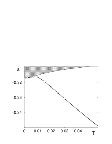
FIG. 3.: Variation of the chemical potential as function of temperature (at $l=\infty$) for $\Delta_{B}=-0.6$, $n_{tot}=1$. The Boson band is shown as a shaded area.

B. The Boson spectrum

Due to the interaction with Fermions the initially localized Bosons acquire itinerancy. The effective interaction between Bosons, being of order $v^{4}$, is hence neglected here. In Figs. 4,5 we show how, with a decrease of temperature, the Boson band becomes broadened and the effective mass of the Bosons $m_{B}$ gets reduced, finally saturating around $m_{B}(T\rightarrow 0)\sim m^{0}_{F}/4$. As a relative quantity we use $m^{0}_{F}=\frac{\hbar^{2}}{2ta^{2}}$ which refers to the bare initial Fermion mass for the $1D$ tight binding case. A parabolic curvature of the long wavelength limit $k\rightarrow 0$ is characterized by the inverse effective mass.

For all temperatures studied by us the Boson dispersion function exhibits a resonant like feature (a kink) around momentum $q=2k^{*}\sim 1.8$. This does not correspond to the value of $2k_{F}$ as was initially mistakenly believed[5]. By inspecting the location of such a kink for other sets of model parameters we conclude that it is mainly depending on the choice of $\Delta_{B}$. This kink occurs for such momenta which satisfy the condition

$$\varepsilon_{k^{*}}+\varepsilon_{q-k^{*}}=E_{q}\;,$$ (58)

where $q$ is a wavevector in the first Brillouin zone. Since within a precision of the order $v^{2}$ the value of the Boson energies is around the initial $\Delta_{B}$, $k^{*}$ is roughly determined by the condition $2\varepsilon_{k^{*}}=\Delta_{B}$. In an approximate study of the flow equations based on a first iterative substitutions (section II. B) one can check that the function $E_{q}$, Eq.(35) in fact diverges for $q=2k^{*}$.

FIG. 4.: The effective Boson dispersion for a chosen set of temperatures. Notice the increase of the band width with a decrease of temperature. At very small temperatures the bottom of the Boson band asymptotically approaches the position of $2\mu$ and as a result the top of the Boson band gets somewhat pushed up.

FIG. 5.: Low temperature behaviour of the effective Bosons mass in units of the initial Fermions mass $m^{0}_{F}$. In the insert we draw the long wavelength limit of the Boson spectrum for the three lowest temperatures evaluated; $T=0.001,0.005,0.007$.

C. Interactions between Fermions

As a result of the renormalization of the model parameters we obtain an effective interaction between Fermions. Figs 6,7 below illustrate the momentum characteristics of the two channels defined in Eqs. (37,38).

Again, we notice certain characteristic features appearing for the momenta corresponding to $k^{*}$. The interaction $U^{(d-d)}_{k,q}$ has a rather regular behaviour: for momenta such that $k^{2}+q^{2}<k^{*2}$ this interaction is attractive, while elsewhere it is repulsive. Around the region $k^{2}+q^{2}=k^{*2}$ we observe a changeover, which looks quite singular.

The interaction $U^{(BCS)}_{k,q}$ shows a similar behaviour as $U^{(d-d)}_{k,q}$ but only along the cross-section $q=k$ (see the top of Fig. 8). Otherwise, the corresponding change-over between the attractive and the repulsive interaction regimes has a smooth character (see the bottom of Fig. 8).

FIG. 6.: The BCS interaction strength $U^{(BCS)}_{k,q}$ for $T=0.001$.

FIG. 7.: the density-density interaction strength $U^{(d-d)}_{k,q}$ for $T=0.001$.

Temperature has a negligible effect on the effective Fermion-Fermion interaction. For example, $U^{(BCS)}_{0,0}$ decreases only by about $0.4\%$ when the temperature is varied from $0.1$ to $0.001$. No qualitative change is observed at all. Nevertheless temperature is an important factor in as far as the effectiveness of this Fermion-Fermion interaction is concerned, since with a decrease of temperature $k_{F}\rightarrow k^{*}$. To see that we refer the reader to consult Fig. 3 keeping in mind that $E_{0}\simeq\Delta_{B}$. As seen from the Figs. 8 the interactions for $|k|<k^{*}$ have attractive character and are strongly enhanced (at least the elements $U_{k,q=k}$) infinitesimally below the momentum $k^{*}$. One would naturally expect strong effects of these interactions if the Fermi vector was located just below $k^{*}$.

FIG. 8.: Cross-sections of the interactions $U_{k,q}^{(BCS)}$ and $U_{k,q}^{(d-d)}$ along a) $q=k$ when both interactions are identical (top figure), and b) for $q=0$ (bottom figure). In general both potentials are repulsive for momenta $k>k^{*}$ and become attractive if $k<k^{*}$.

D. The Fermion spectrum

Studying the Fermion spectrum is a rather complicated issue because on one hand it is affected directly through the flow equations (17,18) and, on the other hand, indirectly through the induced interactions as discussed in the preceding section. The effect of temperature turns out to be a very important factor in this problem. In the physical regime of interest (i.e. when the effect of the Boson - Fermion coupling manifests itself strongly) the Fermi momentum is situated just below $k^{*}$. Upon decreasing the temperature $k_{F}$ moves closer and closer to that value. As a result Fermion - Fermion interactions become more and more effective and eventually may lead to destruction of the quasi-particle nature of those Fermions in this model.

Below, we discuss what kind of fermion spectrum arises purely on the basis of the renormalization of the free particle energies given in Eqs. (17,18). In Fig. 9 we plot the dispersion $\varepsilon_{k}^{(R)}$ versus $k$ and in the inset its derivative with respect to initial $\varepsilon_{k}$. Using this derivative we compute the density of states (DOS)

$$\rho(\omega) = \frac{1}{N}\sum_{k}\delta\left(\omega+\mu-\varepsilon^{(R)}_{k}\right)$$ (59)

$$= \int d\varepsilon\rho^{0}(\varepsilon)\left|\frac{d\varepsilon^{(R)}}{d\varepsilon}\right|^{-1}\delta\left(\omega+\mu-\varepsilon^{(R)}\right)$$ (60)

where $\rho^{0}(\varepsilon)=N^{-1}\sum_{k}\delta\left(\varepsilon-\varepsilon_{k}\right)$ is the initial bare DOS of the Fermions.

FIG. 9.: The renormalized ($l\rightarrow\infty$) Fermion spectrum $\varepsilon^{(R)}_{k}$ for low temperature $T=0.005$. Notice the tendency to form a gap around the Fermi vector.

We notice that below a characteristic temperature $T_{F}^{*}$ (at which the chemical potential starts to be pinned at the bottom of the Boson band) there appears a pseudogap centered around the Fermi level. In our case $T_{F}^{*}\sim 0.125$ in units of the initial bare Fermion bandwidth.

An important question is the qualitative change-over of the pseudogap into a true BCS type gap below the condensation temperature $T_{c}$. This question can be tackled in a reasonably controlled way in the $1D$ case. $T_{c}$ is then identically zero and at $T=0$ all Bosons are condensed in the $q=0$ state. Remember that we are dealing here with an effectively free Bose gas on a lattice, the Boson-Boson interaction - of order $v^{4}$ - being neglected. We thus obtain

$$\frac{d\varepsilon_{k}(l)}{dl} = 4n^{B}_{0}(l)\left(\varepsilon_{k}(l)-\mu(l)\right)|v_{k,-k}(l)|^{2}\;,$$ (61)

$$\frac{dv_{k,-k}(l)}{dl} = -4\left(\varepsilon_{k}(l)-\mu(l)\right)^{2}v_{k,-k}(l)\;,$$ (62)

$$\frac{d\mu(l)}{dl}=\frac{1}{2}\;\frac{dE_{0}(l)}{dl} = -2\frac{1}{N}\sum_{k}|\varepsilon_{k}(l)-\mu(l)|\;|v_{k,-k}|^{2}(l)$$ (63)

which follow from the general flow equations (24-28) in the $T=0$ limit. $n^{B}_{0}(l)$ denotes the concentration of condensed Bosons and $\mu(l)=E_{0}(l)/2$ in this limiting case. We need not find the whole Boson spectrum $E_{q}(l)$ because finite momentum states $E_{q\neq 0}$ are not relevant in the ground state (at least in absence of some external fields).

FIG. 10.: The DOS for the renormalized Fermion spectrum (60) for $T=0.02$ (dotted line), $T=0.01$ (dashed line) and $T=0.005$ (solid line). Upon lowering the temperature a pseudogap forms near the Fermi energy i.e., $(\omega=0)$, caused by the bonding two-Fermion states [22]. Some modification of the DOS is also seen for higher energies which corresponds to the antibonding two-Fermion state [22]. In the inset we compare the results obtained within the present flow equation technique (solid line) with those derived by selfconsistent diagrammatic techniques [5] (dotted line) for $T=0.005$.

The set of Eqs.(61,62,63) is rather straightforward to study because the momentum dependence of the hybridization constant $v_{k,-k}(l)$ enters only through $\varepsilon_{k}(l)$. Hence one can use the effective DOS $\rho(\varepsilon,l)=1/N\sum_{k}\delta(\varepsilon-\varepsilon_{k}(l))$ in Eq. (63). We solve numerically these equations for a fixed total concentration of particles which is subject to the supplementary condition

$$n^{B}_{0}(l)=\frac{1}{2}n_{tot}-\int_{-\infty}^{\mu(l)}d\varepsilon(l)\;\rho(\varepsilon,l).$$ (64)

FIG. 11.: Evolution of the renormalized chemical potential $\mu(l)$ (top) and concentration of Bosons $n^{B}_{0}(l)$ (bottom). Total concentration is kept fixed at $n_{tot}=1$.

FIG. 12.: Difference between the DOS of the interacting $\rho(\omega)$ and of the free system $\rho^{0}(\omega)$ for $n_{tot}=0.6597$ and temperatures displayed in the legend.

Fig. 11 shows how the chemical potential is renormalized through this continuous transformation technique. Notice that its variation is of the order $v^{2}$, as in the case of finite temperatures. The total concentration of Bosons (which are all in the condensate state at $T=0$) is rather weakly affected by renormalization (of the order of 4 $\%$).

The important outcome of this $T=0$ case analysis is seen in the spectrum of Fermions. The asymptotical solution at $l\rightarrow\infty$ yields a true gap in $\varepsilon_{k}^{(R)}$ which is formed around the chemical potential. The size of this gap is in very good agreement with the mean field theory prediction, i.e. $\Delta(T=0)=v\sqrt{n^{B}_{0}}$ (see Fig. 13).

In Fig. 12 we summarize our results obtained sofar in this section and which permit us to make some conjectures as to the evolution of the pseudogap into the true superconducting gap as the temperature is lowered. First of all we notice two distinct energy scales which define these two gaps:

i) the superconducting gap being very sharp and being controlled by the first power in the coupling constant $v$

ii) the pseudogap, being evident in form of humps whose positions slightly move closer together as the temperature decreases, varies with the second power of the coupling constant $v$ (remember that in the normal state our flow equation approach the results obtained are within the order of $v^{2}$).

The relative size of the pseudogap and the zero temperature true gap can vary considerably as a function of the Boson concentration, as can be seen from Fig. 13. In Fig. 12 we have chosen a situation close to the experimental situation in the high $T_{c}$ cuprates where the two gaps are of comparable size.

In the next section we shall show that this same technique, applied to the superconducting state, gives the superconducting gap varying with $v$. It is clear that this difference in the size of these two gaps does not mean that they are of different origin! We shall come back to this question in the last section of this paper.

FIG. 13.: Variation of the true gap at $T=0$ as function of Boson concentration obtained by the flow equation method (solid line) compared with the mean field solution (dashed line). The filled circles show the corresponding magnitude of the pseudogap obtained by the flow equation method for a normal phase at $T=0.01$.

IV The superconducting phase

Bosons are not able to condense at any finite (nonzero) temperature unless the dimensionality of the system is higher than two. In this section we try to reach some preliminary conclusions regarding the superconducting phase of the BFM on the basis of flow equation method. We assume that at least some fraction of the Bose subsystem is in the condensed state; in other words we consider $T<T_{BE}$. We show that the appearance of such a condensate is inevitably related to the formation of a true gap in the Fermion subsystem. Our estimation of this gap is in agreement with the mean field theory result for this model [21].

A. The Fermion Subsystem

Given the existence of a certain fraction of condensed Bosons we put the chemical potential at the $q=0$ level of the Boson energy spectrum, i.e., $\mu(l)=E_{q=0}(l)/2$. In the flow equation for Fermion energies, Eqs. (25) we then have a dominating contribution coming from the $n^{(BE)}_{q=0}$ thermal factor and, as a consequence, can simplify this equation to (which for $T=0$ is exact)

$$\frac{d\varepsilon_{k}(l)}{dl}\simeq 4n^{B}_{0}(T,l)\left(\varepsilon_{k}(l)-\mu(l)\right)|v_{k,-k}(l)|^{2}.$$ (65)

$n^{B}_{0}(T,l)$ denotes the concentration of condensed Bosons at temperature $T$. This equation is coupled to the flow equation for the hybridization coupling $v_{k,-k}$, given in Eq.(62). By inspecting the bottom Fig. 11 we see that the $l$ dependence of the condensate concentration can be dropped, $n^{B}_{0}(T,l)\simeq n^{B}_{0}(T)$. For the strictly three-dimensional system the temperature evolution is given through the standard relation $n^{B}_{0}=n^{B}\left[1-\left(T/T_{BE}\right)^{3/2}\right]$, where $n^{B}$ is the total concentration of Bosons. Similarly, the $l$ dependence of chemical potential can be dropped because of the following arguments: 1) for momenta close to the Fermi surface, the renormalizations of $\varepsilon_{k}(l)$ are of the order of $v\sqrt{n^{B}_{0}(T)}$ while the chemical potential undergoes a renormalizations of the order $v^{2}$ (see top Fig. 11)) for momenta which are far from $k_{F}$ (i.e. in the high energy sector, using a terminology of the renormalization group theory) renormalization is not effective at all (except for the nevralgic $k^{*}$ point which is irrelvant for the purpose of the present discussion).

Thus, without loss of generality and precision, we can rewrite the flow equations in the following from

$$\frac{d\xi(l)}{dl} = 4n^{B}_{0}\xi(l)v^{2}(l)$$ (66)

$$\frac{dv(l)}{dl} = -4\xi^{2}(l)v(l)\;,$$ (67)

from which immediately follows

$$n^{B}_{0}v^{2}(l)+\xi^{2}(l)=const.$$ (68)

where $\xi(l)=\varepsilon(l)-\mu$ measures the Fermion energy from the chemical potential. It is evident from Eq. (50) that for any nonzero $\xi$ the hybridization must evolve to zero in the infinite $l$ limit, $v(\xi\neq 0)\rightarrow 0$. Consequently the renormalized spectrum becomes

$$\varepsilon^{(R)}-\mu={\rm sign}\left(\varepsilon-\mu\right)\;\sqrt{\left(\varepsilon-\mu\right)^{2}+n^{B}_{0}v^{2}}\;.$$ (69)

The gap formed around the chemical potential in the Fermion subsystem is given by

$$\Delta_{F}(T)=v\sqrt{n^{B}_{0}(T)}$$ (70)

which is the same as predicted by our previous studies [19, 21] of this model. This result confirms that the BFM is characterized by a single transition temperature $T_{c}$ at which the Bosons start to condense and Fermions to form a gap in their excitation spectrum. Hence $T_{c}=T^{(B)}_{BE}=T^{(F)}_{BCS}$.

B. The Boson Subsystem

A very important issue in this context is to understand the impact of the gap in the Fermion spectrum on the excitation spectrum of the Bosons. Unfortunately the general flow equation, Eq. (28) can not be handled analytically, not even in the small $q$ limit.

In order to get some insight we study numerically this equation together with the constraint, Eq. (67) which, evidently, applies only for $T<T_{BE}$ and for dimensions larger than two. The set of equations we have then to solve are Eqs. (19,22) together with

$$\left[\varepsilon_{k}(l)-\mu(l)\right]^{2}=\left[\varepsilon_{k}-\mu\right]^{2}+n^{B}_{0}\left[v^{2}-|v_{k,-k}(l)|^{2}\right]\;$$ (71)

which is a direct consequence of the constraint, Eq (51). We fix the chemical potential at the level $\mu(l)=E_{q=0}(l)/2$ throughout the iterative solution procedure. Eq. (71) controls the formation of the gap in the Fermion spectrum as a result of the presence of Boson in the condensate. With the constraint, Eq. (71) included, we investigate the Boson spectrum $E_{q}$ by restricting ourselves to performing a one-dimensional momentum summation in Eq. (28). Such an approximative procedure reduces considerably the numerical complexity and is expected to give at least qualitatively correct results for dimensionality larger than two. A complete numerical study on this point will be reported in some future work.

FIG. 14.: Momentum characteristics of the Boson excitation spectrum in the superfluid state of the BFM with $n_{tot}=1$. Solid lines correspond to various temperatures as marked and the dotted line is taken from the selfconsistent solution for the normal phase at $T=0.005$. Inset: the same function for the superfluid (solid line) and normal phase (dotted line) within the half Brillouin zone at $T=0.005$.

FIG. 15.: Sound velocity and the condensate concentration versus $T$ for the superfluid phase of the BFM with $n_{tot}=1$.

¿From the numerical analysis of the above flow equations we obtain $E_{q}$. In the long wavelength limit ($q\rightarrow 0$) it significantly deviates from its behavior, obtained above, in the normal state. In order to illustrate this, we plot in Fig. 14 the momentum dependence of $\left[E^{(R)}_{q}-E^{(R)}_{q=0}\right]/q$ for several temperatures. Clearly the curves show linear behavior up to momenta $q\sim 0.15$ and, what is more important, show a non-zero crossing point with the ordinate. Its value determines the sound velocity $v_{s}(T)$ and marks the presence of a collective excitation in the superfluid Bose subsystem. That such a sound wave mode is completely absent in the normal phase can be seen by the dashed line in Fig. 14 which crosses the ordinate at zero.

By inspection of Fig. 14 one notices the decrease of the sound velocity with increasing temperature. Simultaneously the region of the $q^{2}$ behavior of the spectrum starts to shrink. In Figs. (15,16) we show the dependence of the sound velocity versus temperature (for a total concentration of carriers $n_{tot}=1$) and versus total concentration at $T=0.0$. These results agree well with the predictions for the BFM obtained earlier by means of the dielectric function formalism[21]. In the so-called Bose limit, i.e. when the concentration of Bosons is not small, the sound velocity has been shown to gradually decrease with an increase of temperature towards $T_{c}$. On the other hand, the sound velocity of the ground state gets reduced when the total concentration of carriers increases (see Fig. 15 of our present calculations and compare with Fig. 2 of Ref. [21]). Only in the dilute regime for small Boson concentrations (the so called BCS limit) one expects a behavior, qualitatively different from that studied here.

FIG. 16.: Sound velocity of the ground state $T=0$ as a function of total concentration $n_{tot}$ for $\Delta_{B}=-0.6$. Notice that critical concentration above which superfluidity (superconductivity) can arise is roughly equal $n_{cr}\sim 0.49$.

V Conclusion

Our previous studies[5] of the BFM indicated that the superconducting features of it arise due to the initially localized Bosons becoming itinerant, an effect which is triggered by a mutual feedback effect between the two subsystems. Concomitantely with this occurs the formation of a pseudogap in the DOS of the Fermions, as the temperature is lowered and which in turn permits the Bosons to acquire longer and longer lifetimes. The reason for that is a reduction of scattering processes due to a diminishing number of Fermionic states available in this energy region. The opening of the pseudogap in those descriptions is linked to a renormalized Fermion dispersion which becomes flat as the Fermi energy is approached from below, but, with at the same time, a substantial loss in spectral weight and lifetime broadening [24]. The end result is in effect a separation into two separate subsystems, the Fermionic and the Bosonic one with their proper dynamics. Yet, due to the exchange coupling, they are mutually dependent on each other which leads to a single critical temperature, describing the onset of superconductivity, in both of the two effective uncoupled subsystems.

The flow-equation technique studied in this work, renormalizes this inter-subsystem coupling to zero and hence is capable to make this interdependence of the dynamics of these two subsystems explicit. The various results obtained here are correct to second order in the initial unrenormalized inter-subsystem coupling constant $v$. The effective Bosonic subsystem behaves essentially as a lattice gas of free Bosons with a temperature dependent mass. The effective Fermion subsystem shows a dispersion which, upon approaching the Fermi wavevector rises almost vertically to some value above the Fermi energy within a very small regime around $k_{F}$. This reflects a pseudogap structure in the DOS which is of order $v^{2}$. In this regime of energies the effective renormalized intra-subsystem interaction is very singular (see Figs. (6 -8)) and is expected to give rise to the lifetime effects and the reduction in spectral weight seen on our previous studies[5]. For wavevectors greater than $k_{F}$ the effective Fermion dispersion remains quasi unrenormalized.

The use of the flow equation technique enables us to treat the superconducting and the normal state on the same footing and, on the basis of that, to make some conjectures as to how the pseudogap evolves into the true gap in the superconducting phase. For a $1D$ system where the superconducting phase is realized at $T\equiv 0$ the pseudogap evolves in from of a $V$-shaped curve which deepens until it touches the zero density level upon decreasing the temperature towards $T=0^{+}$. Upon entering the superconducting state at exactly $T=0$, this $V$ shaped curve changes abruptly into a more conventional $U$ shaped curve, known from standard BCS type superconductors. The pseudogap is characterized by two distinct humplike features in the DOS whose positions get slowly closer to each other as the temperature is decreased. The energy difference between those two humps being of the order of $v^{2}$. These pseudogap features are distinctively different from the gap structure in the superconducting state, as can be seen from Fig.12. The superconducting gap shows a different variation with the inter-subsytem coupling constant, varying as $v$. The sizes for the pseudo- and the superconducting gap can in principle be quite different, as shown in Fig. 13. This does not mean that they are of different physical origin. We know from our previous studies[2] that the pseudogap is very much independent on dimensionality, while the superconducting gap evidently is dependent on it. The present study, further, suggests that the variation of the two gaps with the concentration of Bosons varies in opposite direction. This can lead to a situation of a coexistence of two gap like structures in the superconducting phase, i.e., a superconducting gap and a remnant of the pseudogap. To what extent we should consider the pseudogap as a precursor of the superconducting is a question of semantics. For the model system considered here, as well as for the real High $T_{c}$ cuprate materials the pseudogap is caused by amplitude rather than phase fluctuations. Amplitude fluctuations are a prerequisite of the superconducting state but are not by themselves sufficient to guarantee its materialization. As a consequence, upon reducing the dimensionality of the system, the superconducting state is suppressed and tends to an insulating state with a characteristic upturn of the resistivity at low temperatures[2].

The study of the change-over between the pseudogap and the superconducting gap for the more realistic anisotropic $3D$ case, together with a careful study of the lifetime effects controlled by the intra-Fermion subsystem interactions is presently under investigation and will be reported in some future study.

Finally, for reasons of completeness, we should mention the theoretical studies of the pseudogap phenomenon based on the so-called BCS-Bose Einstein cross-over scenario. Such studies are based on effective BCS type coupling as well as the negative U Hubbard model[25]. Within this approach similar questions of a change-over form the pseudogap into a true gap have been considered[26]. A discussion the precise differences between this scenario and the BFM scenario as concerns the physics and applicability to the High $T_{c}$ cuprates lies outside the frame of subject discussed in the present paper.

VI Acknowledgement

T.D. would like to acknowledge financial support from the University Joseph Fourier, Grenoble, and the hospitatily of the Centre de recherche pour les tres basses temperatures where this work was carried out. Moreover T.D. acknowledges support from the Polish Committee of Scientific Research under the grant No 2P03B10618.

Appendix

Let us consider the following modification of the generating operator

$$\tilde{\eta}=\eta+\eta^{(2)}$$ (72)

where $\eta$ is given by equation (9) and where we choose

$$\eta^{(2)}=\frac{1}{N}\sum_{\sigma}\sum_{p,k,q\neq k}\left(\gamma^{\sigma}_{p,k,q}(l)b^{\dagger}_{p+q}b_{p+k}c^{\dagger}_{k\sigma}c_{q\sigma}-{\rm h.c.}\right).$$ (73)

The coefficients $\gamma^{\sigma}_{p,k,q}(l)$ can be selected in any arbitrary way provided that $v_{k,p}(l\rightarrow\infty)\rightarrow 0$ still holds.

By a straightforward calculations one verifies that

$$\left[\eta^{(2)},H\right]=\frac{1}{N}\sum_{\sigma}\sum_{p,k,q\neq k}\left(E_{p+k}-E_{p+q}-\varepsilon^{\sigma}_{k}+\varepsilon^{\sigma}_{q}\right)$$ (74)

$$\times\left(\gamma^{\sigma}_{p,k,q}b^{\dagger}_{p+q}b_{p+k}c^{\dagger}_{k\sigma}c_{q\sigma}+{\rm h.c.}\right)+O(\gamma v,\gamma U).$$ (75)

If we now use the Ansatz

$$\gamma^{\downarrow}_{p,k,q}(l) = -\;\frac{\varepsilon^{\downarrow}_{k}+\varepsilon^{\uparrow}_{p}-E_{p+k}}{E_{p+k}-E_{p+q}-\varepsilon^{\downarrow}_{k}+\varepsilon^{\downarrow}_{q}}\;\;v^{*}_{k,p}v_{q,p}$$ (76)

$$\gamma^{\uparrow}_{p,k,q}(l) = -\;\frac{\varepsilon^{\downarrow}_{p}+\varepsilon^{\uparrow}_{k}-E_{p+k}}{E_{p+k}-E_{p+q}-\varepsilon^{\uparrow}_{k}+\varepsilon^{\uparrow}_{q}}\;\;v^{*}_{p,k}v_{p,q}$$ (77)

then we effectively obtain

$$\left[\eta^{(2)},H\right]=-\frac{1}{N}\sum_{p,k,q\neq k}b^{\dagger}_{p+q}b_{p+k}\left[\left(\alpha_{k,p}+\alpha_{q,p}\right)v^{*}_{k,p}v_{q,p}\right.$$ (78)

$$\times\left.c^{\dagger}_{k\downarrow}c_{q\downarrow}+\left(\alpha_{p,k}+\alpha_{p,q}\right)v^{*}_{p,k}v_{p,q}c^{\dagger}_{k\uparrow}c_{q\uparrow}\right]+O(v^{3})\;.$$ (79)

The terms containing $\gamma v$ become of the order $O(v^{3})$ and from the flow equation (29) we can estimate $U\sim v^{2}$ which yields that $\gamma U\sim O(v^{4})$.

Thus on the right hand side of equation (79) we obtain the same term as in (20) but with an opposite sign. These terms subtract each other if one uses $\tilde{\eta}$ in the flow equation instead of the initial one (9). The modified continuous unitary transformation does not generate any interaction of the form $b^{\dagger}_{p+q}b_{p+k}c^{\dagger}_{k\sigma}c_{q\sigma}$ for $q\neq k$ unless hybridization constant $v$ is large enough.

REFERENCES

- [1] A. Georges, G. Kotliar, W. Krauth and M. Rozenberg, Rev. Mod. Phys. 68, 13 (1996); F. Gebhard, ”The Mott Metal Insulator transition”, Springer Verlag, 1997.
- [2] J.-M. Robin, A. Romano and J. Ranninger, Phys. Rev. Lett. 81, 2756 (1998); A. Romano and J. Ranninger, Phys. Rev. B (Aug. 1. (2000)); cond-mat/0005295.
- [3] Y. Motome and G. Kotliar, cond-mat/0005395.
- [4] G. M. Eliashberg, Zh. Eksp.. Teor. Fiz. 28, 966 (1960); ibid. 29 1437 (1990) [Sov. Physics JETP 11, 696 (1960), ibid. 12 1000 (1960)].
- [5] J. Ranninger, J.-M. Robin and M. Eschrig, Phys. Rev. Lett. 74, 4027 (1995); P. Devillard and J. Ranninger, Phys. Rev. Lett. 84, 5200 (2000).
- [6] S.D. Głazek and K.G. Wilson, Phys. Rev. D 48, 5863 (1994).
- [7] F. Wegner, Ann. Physik 3, 77 (1994).
- [8] A. Mielke, Eur. Phys. J. B, 605 (1998).
- [9] S.K. Kehrein and A. Mielke, J. Phys. A: Math. Gen. 27, 4257 (1994).
-
[10]
P. Lenz and F. Wegner, Nucl. Phys. B 482
[FS], 693 (1996);
A. Mielke, Ann. Physik 6, 215 (1997);
A. Mielke, Europhys. Lett. 40, 195 (1997) - [11] S.K. Kehrein and A. Mielke, Annals of Phys. 252, 1 (1996)
- [12] J. Stein, J. Statistical Phys. 88, 487 (1997).
- [13] J. Stein, Eur. Phys. J. B 5, 193 (1998).
-
[14]
S.K. Kehrein and A. Mielke,
Z. Phys. B 99, 269 (1996);
Phys. Lett. A 219, 313 (1996); Ann. Physik 6, 91 (1997). - [15] K.G. Wilson et al, Phys. Rev. D 49, 6720 (1997).
- [16] M.M. Brisudova, R. J. Perry and K.G. Wilson, Phys. Rev. Lett. 78, 1227 (1997).
- [17] S. Kehrein, Phys. Rev. Lett. 83, 4914 (1999).
- [18] M. Ragawitz and F. Wegner, Eur. Phys. J. B 8, 9 (1999).
- [19] J. Ranninger and J.M. Robin, Phys. Rev. B B 56, 8330 (1997).
- [20] H.C. Ren, Physica C 303, 115 (1998).
- [21] T. Kostyrko and J. Ranninger, Phys. Rev. B 54 (1996) 13 105.
- [22] T. Domanski, J. Ranninger and J. -M. Robin, Solid State Commun. 105, 473 (1998).
- [23] J. Ranninger and J. -M. Robin, Physica C 253, 279 (1995).
- [24] J. Ranninger and J. -M. Robin, Solid State Commun. 98, 559 (1996).
- [25] M. Randeria, Proc. Int. School of Physics ”Enrico Fermi”, Course CXXXVI,”Models and phenomenology for conventional and High-temperature Superconductivity”, eds. G. Iadonisi, R. Schrieffer and M.L. Chiofalo, Varenna (1997) (IOS Press, Amsterdam, 1998) pp. 53-75; R. Micnas, M.H. Pedersen, S. Schafroth, T. Schneider, J.J.Rodriguez-Nunez and H. Beck, Phys. Rev. B 52, 16223 (1995); M. Letz and R. J. Gooding, J. Phys.: Condens. Matter 10, 6931 (1998).
- [26] O. Tchernyshyov, Phys. Rev. B 56, 3372 (1997); I. Kosztin, Q. Chen, B. Janko and K. Levin, Phys. Rev. B 58, R5936 (1998).