Temporal correlations and persistence in the kinetic Ising model: the role of temperature

Abstract

We study the statistical properties of the sum $S_{t}=\int_{0}^{t}dt^{\prime}\,\sigma_{t^{\prime}}$, that is the difference of time spent positive or negative by the spin $\sigma_{t}$, located at a given site of a $D$-dimensional Ising model evolving under Glauber dynamics from a random initial configuration. We investigate the distribution of $S_{t}$ and the first-passage statistics (persistence) of this quantity. We discuss successively the three regimes of high temperature ($T>T_{c}$), criticality ($T=T_{c}$), and low temperature ($T<T_{c}$). We discuss in particular the question of the temperature dependence of the persistence exponent $\theta$, as well as that of the spectrum of exponents $\theta(x)$, in the low temperature phase. The probability that the temporal mean $S_{t}/t$ was always larger than the equilibrium magnetization is found to decay as $t^{-\theta-\frac{1}{2}}$. This yields a numerical determination of the persistence exponent $\theta$ in the whole low temperature phase, in two dimensions, and above the roughening transition, in the low-temperature phase of the three-dimensional Ising model.

1 Introduction

Consider a $D$-dimensional lattice of Ising spins, evolving under Glauber dynamics at a fixed temperature $T$ from a random initial configuration. This is obtained e.g. by quenching the system from very high temperature down to $T$. The purpose of this work is to study the influence of temperature on the statistical properties of the sum

$$S_{t}=\int_{0}^{t}dt^{\prime}\,\sigma_{t^{\prime}},$$ (1.1)

where $\sigma_{t}=\pm 1$ is the spin at a given site. More precisely, we shall investigate two facets of this problem:

• the scaling of $S_{t}$ with $t$, and more generally the bulk properties of the distribution of $S_{t}$,

• the statistics of rare events (such as large deviations, first passages, persistence), i.e. the tail properties of this distribution.

Equivalent writings of the sum are $S_{t}=T_{t}^{+}-T_{t}^{-}=t\,M_{t}$, where

$$T_{t}^{\pm}=\int_{0}^{t}dt^{\prime}\,\frac{1\pm\sigma_{t^{\prime}}}{2}$$

are the lengths of time spent by the spin $\sigma_{t}$ in the positive (negative) direction, or occupation times of the $\pm$ states, with $T_{t}^{+}+T_{t}^{-}=t$, and $M_{t}$ is the temporal mean of $\sigma_{t}$, or local mean magnetization. If one views $\sigma_{t}$ as the steps of a fictitious random walker, then $S_{t}$ is the position of the random walker at time $t$, and $M_{t}$ its mean speed.

Simple as it may seem, the problem thus stated is actually very intricate. The reason is that, the values of $\sigma_{t}$ at different instants of time being in general correlated, this study pertains to that of sums of correlated random variables, for which no universal result exists. The central limit theorem holds only for weakly correlated random variables. As we shall see, $S_{t}$ obeys the central limit theorem for $T>T_{c}$, while the latter is violated for $T\leq T_{c}$.

Hereafter, we focus our attention on the asymptotic behaviour of the following quantities, as $t\rightarrow\infty$.
(i) The probability distribution of $S_{t}$, or alternatively that of $M_{t}$,given by

$$P(t,x)={\mathcal{P}}\left(\frac{S_{t}}{t}>x\right)\qquad(-1<x<1),$$ (1.2)

with corresponding densities, related by

$$f_{M}(t,x)=t\,f_{S}(t,y=tx)=-\frac{d}{dx}P(t,x).$$

Assume that the typical value of $S_{t}$ scales, for long times, as $t^{\alpha}$. By definition of $S_{t}$, $\alpha\leq 1$ necessarily. Then, if $\alpha<1$, the events $\{S_{t}>tx\}$, with $x>0$, are rare. (Or the events $\{S_{t}<tx\}$ with $x<0$.) The tail probability $P(t,x)$, which measures their weight, is vanishingly small, as $t\to\infty$. In contrast, if $\alpha=1$, $P(t,x)$ is expected to converge to a limiting distribution, i.e., the distribution of $S_{t}$ has fat tails. The former case corresponds to $T\geq T_{c}$, the latter to $T<T_{c}$, as detailed below.

(ii) The first-passage probability

$$R(t,x)={\mathcal{P}}\left(\frac{S_{t^{\prime}}}{t^{\prime}}>x,\textrm{}{forall}t^{\prime}\leq t\right)\qquad(-1<x<1),$$ (1.3)

which is the probability for the random walker not to cross the line $S_{t^{\prime}}=t^{\prime}x$, up to time $t$. This is also referred to as the probability of persistent large deviations, sinceit involves the large-deviation event $\{S_{t}/t>x\}$, and the persistence condition $\{$for all $t^{\prime}\leq t\}$.

Special cases of these quantities are, first, the probability of first passage of $S_{t}$ by the origin

$$R(t,0)={\mathcal{P}}(S_{t^{\prime}}>0,\textrm{}{forall}t^{\prime}\leq t),$$ (1.4)

and, secondly, the persistence probability of the process $\sigma_{t}$ (assuming that $\sigma_{t=0}=+1$)

$$p_{0}(t)={\mathcal{P}}(\textrm{}{noflipof}\sigma_{t^{\prime}},\textrm{}{forall}t^{\prime}\leq t)\equiv{\mathcal{P}}\left(S_{t}=t\right),$$ (1.5)

which is also formally equal to $R(t,x=1)$.

The principal motivation behind such an investigation comes from the problem of phase persistence, where, for a system undergoing phase ordering, the question posed is: “What is the probability for a given point of space to remain in the same phase as time passes?”.

For the particular case of $T=0$, say for a spin model, the question above is answered by the knowledge of $p_{0}(t)$, which decays at long times as $t^{-\theta}$, thus defining the persistence exponent $\theta$ [1]. However, as shown in [2], consideration of the more general events $\{S_{t}/t>x\}$, beyond that of the most extreme event $\{S_{t}=t\}$ (the spin never flipped), allows both a stationary definition of the persistence exponent $\theta$, as the edge singularity of $\lim_{t\to\infty}P(t,x)$, for $x\to\pm 1$, and the introduction of a whole spectrum of exponents $\theta(x)$, through the temporal decay of $R(t,x)$. The interest of introducing such concepts is strengthened by the fact that, for $0<T<T_{c}$, the same definition of the persistence exponent holds, now for $x\to\pm m_{{\rm eq}}$ [3] (see below).

In essence, the change in viewpoint when considering $P(t,x)$ and $R(t,x)$ instead of $p_{0}(t)$ amounts to shifting from the original question posed above to the more general one: “How long did the system remain in a given phase?”. This means in particular searching the distribution of the length of time spent by the system inthe given phase, or occupation time of the phase, directly related to the sum (1.1). The statistics of the occupation time provides information on the ergodic nature of the process. Further developments on this theme can be found in refs. [4] to [13].

This work is a sequel and a completion of [3]. We investigate the behaviour of the distribution of $S_{t}$ and of $R(t,x)$ in the three temperature regimes, $T>T_{c}$, $T=T_{c}$, and $T<T_{c}$, and in particular revisit the question of the definition of the persistence exponent in the low-temperature phase. We will mainly consider here the two-dimensional case, and incidentally comment on the case $D=3$.

2 Temperature regimes

In its heat-bath formulation, Glauber dynamics consists in updating the spin $\sigma_{t}$, located at a given site, with the probability

$${\mathcal{P}}\left(\sigma_{t+dt}=+1\right)=\frac{1}{2}\left(1+\tanh\frac{h_{t}}{T}\right),$$ (2.1)

where $h_{t}$ is the local field at the given site, equal to the sum of the neighbouring spins. Under this dynamics spins thermalize in their local environment.

The behaviour of the system is qualitatively different according to the value of the temperature at which the dynamics takes place, that is the temperature $T$ after the quench. Three regimes are observed when letting $T$ vary from high ($T>T_{c}$) to low temperatures ($T<T_{c}$). An overview of the changes in behaviour with temperature is given in figure 1, which depicts samples of spin histories, i.e., the position $S_{t}$ of the Ising random walk as a function of time, for $0<t<1000$, together with the corresponding distributions of $S_{t}$ at time $t=1000$, as temperature varies. The top pictures correspond to a sample of 30 spins located at various sites of a two-dimensional $4096^{2}$ square lattice, the bottom pictures to all the spins of the lattice. ($T_{c}^{2D}=2/\ln(1+\sqrt{2})\approx 2.269$.)

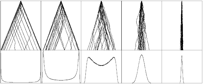
Figure 1: Top curves: samples of spin histories. From left to right: $T=0$, $T=0.9\,T_{c}$, $T=T_{c}$, $T=1.1\,T_{c}$, $T=\infty$. The vertical axis is time ($0<t<1000$), the horizontal axis represents $S_{t}$, the position of the Ising random walk. Bottom curves: unnormalized histograms of $S_{t}$, at time $t=1000$. (The system size is $4096^{2}$.)

Snapshots at time $t=1000$ of spin configurations and of configurations of the values of $S_{t}$ for various temperatures are given in figures 2 and 3.

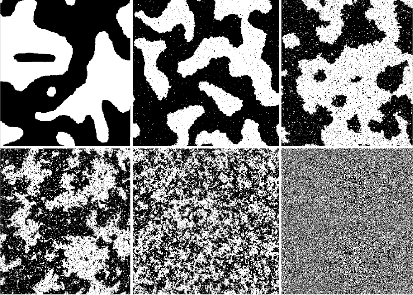
Figure 2: Snapshots at time $t=1000$ of spin configurations for various temperatures. From top left to bottom right: $T=0$, $0.7\,T_{c}$, $0.9\,T_{c}$, $T_{c}$, $1.1\,T_{c}$, and $T=\infty$.

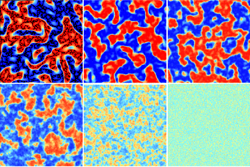
Figure 3: Snapshots at time $t=1000$ of configurations of the values of $S_{t}$ for various temperatures. From top left to bottom right: $T=0$, $0.7\,T_{c}$, $0.9\,T_{c}$, $T_{c}$, $1.1\,T_{c}$, and $T=\infty$. Values of $S_{t}$ ranging from $-1000$ to $1000$ are represented by colours ranging from dark blue to dark red. Persistent spins ($S_{t}=\pm 1000$), present in the top left picture ($T=0$) only, are represented in black.

2.1 High temperature

As long as $T>T_{c}$, thermal equilibrium is attained exponentially fast (with a finite relaxation time $t_{\mathrm{eq}}$). The equilibrium magnetization $m_{\mathrm{eq}}$ of the system is equal to $0$.

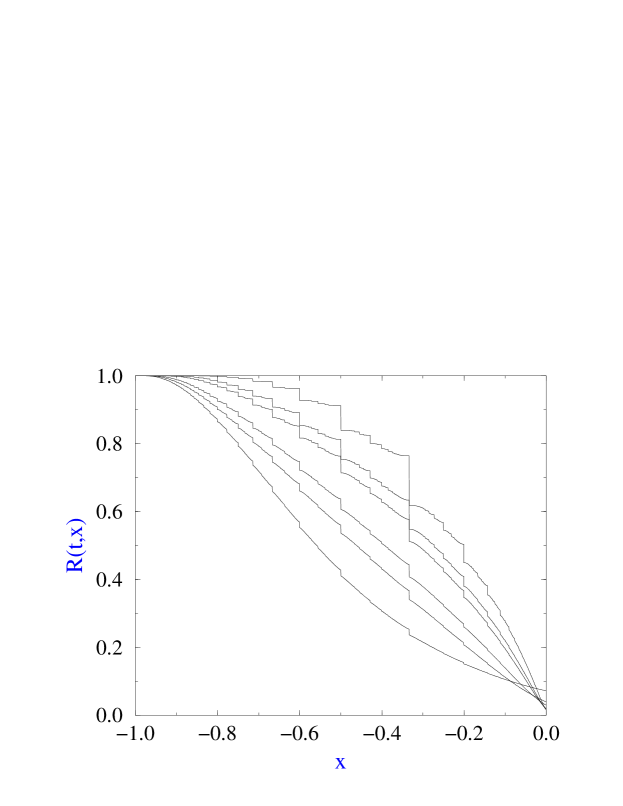
Figure 4: $R(t=10000,x)$ in the high temperature phase, for $-1<x<0$. From top to bottom: $T=\infty$, $1.5\,T_{c}$, $1.3\,T_{c}$, $1.1\,T_{c}$, $1.05\,T_{c}$, $1.01\,T_{c}$. (The system size is $4096^{2}$.)

Let us first consider the simplest case $T=\infty$. The values of the spin $\sigma_{t}$ at successive instants of time are independent and equiprobable, as the steps of a binomial random walk in continuous time, hence $S_{t}$ is a sum of independent, identically distributed random variables. Therefore the central limit theorem holds. The typical value of $S_{t}$ reads

$$(S_{t})_{\mathrm{typ}}\sim t^{\frac{1}{2}},$$

and the limiting distribution of $S_{t}/t^{1/2}$ is Gaussian. More precisely, the bulk of the distribution reads

$$P(t,x=t^{-\frac{1}{2}}z)={\mathcal{P}}\left(t^{-\frac{1}{2}}S_{t}>z\right)\sim\int_{z}^{\infty}du\,\exp\left(-\frac{u^{2}}{2}\right),$$

because the variance of $S_{t}$ equals $t$. Hence, for (the bulk of) the density of $M_{t}$, we have

$$f_{M}(t,x)\sim t^{\frac{1}{2}}\exp\left(-\frac{t\,x^{2}}{2}\right).$$ (2.2)

Figure 1 gives an illustration of the random walk associated to $S_{t}$, and of the Gaussian distribution of this quantity at $T=\infty$ (first pictures from the right).

If $t$ is large, and $x>0$, $P(t,x)$ measures the probability of the rare events such that $S_{t}\sim t$, or $M_{t}\sim O(1)$, i.e., of large deviations of $S_{t}$ with respect to its typical behaviour. For any sum $S_{t}$ of independent, identically distributed random variables, the tail of $P(t,x)$ (probability of a large deviation) is given by

$$P(t,x)\mathrel{\mathop{\sim}\limits_{t\to\infty}}\exp\left(-I(x)\,t\right)\qquad(x>0).$$ (2.3)

In the present case, $T=\infty$, that is for a binomial random walk (with equiprobable steps $\pm 1$), we have $I(x)=\frac{1}{2}[(1+x)\ln(1+x)$ $+(1-x)\ln(1-x)]$. (For a simple derivation see [2].) For $x\rightarrow 0$, $I(x)\approx x^{2}/2$, the scaling variable is $x^{2}t=z^{2}$, hence the central limit theorem is recovered.

For a sum $S_{t}$ of independent random variables, the probability of first passage by the origin, ${\mathcal{P}}(S_{t^{\prime}}>0,$ for all $t^{\prime}\leq t)$, decays as $t^{-\frac{1}{2}}$, as is well known. The behaviour of $R(t,x)$, for $x\neq 0$, is more subtle. According to ref. [6] we have, for a binomial random walk, as $t\rightarrow\infty$,

$$R(t,x)\sim\left\{\begin{array}[]{l}\exp\left(-I(x)t\right)\\ t^{-\frac{1}{2}}\\ R_{\infty}(x)\end{array}\begin{array}[]{l}0<x<1\\ x=0\\ -1<x<0\end{array}\right..$$ (2.4)

The asymptotic value $R_{\infty}(x)$ is the top curve of figure 4. It is obtained by taking the value at time $t=10000$ of $R(t,x)$ for $T=\infty$, depicted in figure 5 (left). The devil’s staircase thus obtained, a discontinuous curve at all the rationals, is indistinguishable from its analytical prediction given in ref. [6].

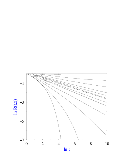
Figure 5: $R(t,x)$ at $T=\infty$ (left) and $T=T_{c}$ (right).
For $T=\infty$, from bottom to top: $x=$ 1, 0.8, 0.6, 0.4, 0.2, 0.1, 0.02, 0, $-0.02$, $-0.1$, $-0.2$, $-0.4$, $-0.6$, $-0.8$. The dashed line parallel to $R(t,0)$ has slope $-\theta(0)=-\frac{1}{2}$.
For $T=T_{c}$, from bottom to top: $x=$1, 0.8, 0.6, 0.4, 0.2, 0.1, 0, $-0.1$, $-0.2$, $-0.4$, $-0.6$, $-0.8$. The dashed line parallel to $R(t,0)$ has slope $-\theta(0)=-0.273$. (The system size is $4096^{2}$.)

The persistence probability $p_{0}(t)$ behaves, as $t\rightarrow\infty$, as $p_{0}(t)\sim\mathrm{e}^{-(\ln 2)\,t}$, which matches both (2.3) and (2.4) for $x=1$. Note that (2.4) defines the first-passage exponent $\theta(x=0)=\frac{1}{2}$.

Let us now investigate the deformations induced on the quantities considered above, when $T$ decreases.

If $T_{c}<T<\infty$, the two-time autocorrelation $\left\langle\sigma_{s}\sigma_{t}\right\rangle$ (with $s<t$) is short ranged. At equilibrium, i.e., for $1\ll s$, $\left\langle\sigma_{s}\sigma_{t}\right\rangle\sim\exp\left(-(t-s)/t_{\mathrm{eq}}\right)$. Hence the statistics of $S_{t}$ is that of a random walk with short-ranged correlations, and the central limit theorem still holds. The distribution of $S_{t}$ is Gaussian (see second pictures from the right in figure 1, for $T=1.1\,T_{c}$), with a width proportional to $(t\,t_{{\rm eq}})^{\frac{1}{2}}$. While the Gaussian shape of $P(t,x)$ in the bulk is universal, as long as the correlations $\left\langle\sigma_{s}\sigma_{t}\right\rangle$ are short-ranged, the tails are not. Hence $I(x)$ is expected to be deformed as $T$ decreases from infinity to $T_{c}$.

The probability of first passage by the origin, ${\mathcal{P}}(S_{t^{\prime}}>0,$ for all $t^{\prime}\leq t)$, still decays as $t^{-\frac{1}{2}}$. The persistence probability $R(t,x)$ behaves qualitatively as in equation (2.4). As $T$ decreases down to $T_{c}$, the discontinuous curve $R_{\infty}(x)$ is deformed, as seen in figure 4. Gaps vanish when $T\to T_{c}$. Note the finite time effect when approaching $T_{c}$, manifested by the fact that $R_{\infty}(x)$ does not vanish as $x\rightarrow 0$.

2.2 Critical coarsening

The system is now quenched from a disordered initial state to its critical point.

After the quench, spatial correlations develop in the system, just as in the critical state, but only over a length scale which grows like $t^{1/z_{c}}$, where $z_{c}$ is the dynamic critical exponent. The equal-time correlation function has the scaling form

$$C_{\mathbf{x}}(t)=\left\langle\sigma_{t}(0)\sigma_{t}({\mathbf{x}})\right\rangle=|{\mathbf{x}}|^{-2\beta/\nu}\,\phi\!\left(\frac{|{\mathbf{x}}|}{t^{1/z_{c}}}\right),$$

where $\mathbf{x}$ is a lattice point, and $\beta$ and $\nu$ are the usual static critical exponents. The scaling function $\phi(y)$ goes to a constant for $y\to 0$, while it falls off exponentially to zero for $x\to\infty$, i.e., on scales smaller than $t^{1/z_{c}}$ the system looks critical, while on larger scales it is disordered. In two dimensions $z_{c}\approx 2.17$, $\beta=\frac{1}{8}$, and $\nu=1$; in three dimensions $z_{c}\approx 2.04$, $\beta\approx 0.327$, and $\nu\approx 0.63$ [14].

Figure 6: Critical scaling function $\varphi$ obtained by rescaling $f_{M}(t,x)$ for three different times: $t=$100, 1000, 10000, see equation (2.7). (The system size is $4096^{2}$.)

For $1\ll s\sim t$ the two-time autocorrelation function scales as [15, 16]

$$C(t,s)=\left\langle\sigma_{s}\sigma_{t}\right\rangle=s^{-2\beta/\nu z_{c}}\,g_{c}\left(\frac{s}{t}\right).$$ (2.5)

A numerical determination of the scaling function $g_{c}$ can be found in ref. [16]. This implies, setting $a=2\beta/\nu z_{c}$,

$$\left\langle M_{t}^{2}\right\rangle = \frac{2}{t^{2}}\int_{0}^{t}dt_{2}\int_{0}^{t_{2}}dt_{1}\,\left\langle\sigma_{t_{1}}\sigma_{t_{2}}\right\rangle$$

$$= 2t^{-a}\,\int_{0}^{1}dv\int_{0}^{v}du\,u^{-a}\,g_{c}\left(\frac{u}{v}\right)$$

$$= t^{-a}\left(\frac{2}{2-a}\int_{0}^{1}dx\,x^{-a}g_{c}(x)\right),$$

hence

$$(S_{t})_{\mathrm{typ}}\sim t^{1-\beta/\nu z_{c}}.$$ (2.6)

Note that this scaling behaviour was obtained from the non-stationary form (2.5). The behaviour of $S_{t}$ at criticality is illustrated by the middle pictures of figure 1.

From equation (2.6) one can infer that the bulk of the probability density of $M_{t}$ scales as

$$f_{M}(t,x)\sim t^{\beta/\nu z_{c}}\varphi(t^{\beta/\nu z_{c}}\,x),$$ (2.7)

which is the critical counterpart of (2.2). The scaling function $\varphi$ is depicted in figure 6, for $D=2$, with $\beta/\nu z_{c}\approx 0.0576$. Due to the smallness of this exponent, $f_{M}$ is very slowly peaking. The existence of the scaling form (2.7) implies gap scaling for higher moments, i.e., $\left\langle M_{t}^{2k}\right\rangle\sim\left\langle M_{t}^{2}\right\rangle^{k}$.

The probability $R(t,x)$ behaves qualitatively as in the high temperature phase (see figure 5, right). For $0<x<1$, it decreases to zero faster than a power-law (in particular $p_{0}(t)\equiv R(t,x=1)$). For $-1<x<0$, it decreases, extremely slowly, to a constant $R_{\infty}(x)$ obtained by extrapolating the results of figure 4, as $T\rightarrow T_{c}$. Finally for $x=0$, $R(t,x)\sim t^{-\theta(0)}$. We find $\theta(0)\approx 0.27$ in 2D and $\theta(0)\approx 0.41$ in 3D. Note that $\theta(0)$ is a nonequilibrium critical exponent.

Remark. The exponent $\theta(0)$ can also be measured at criticality for the two-dimensional $p_{1}-p_{2}$ model [17, 18]. This model is defined as follows. The right side of (2.1), $p(h)=\frac{1}{2}(1+\tanh h/T)$, is a function of $h$ ($h=\pm 4,\pm 2,0$), such that $p(-h)=1-p(h)$. In particular $p(0)=\frac{1}{2}$. The dynamics of the Ising model therefore depends on one parameter only, which is $p_{1}=p(2)$, or alternatively $p_{2}=p(4)$, the two being related. Considering instead these two quantities as independent ($\frac{1}{2}\leq p_{1},p_{2}\leq 1$) defines the $p_{1}-p_{2}$ model. For the voter model ($p_{1}=\frac{3}{4}$, $p_{2}=1$) one finds $\theta(0)\approx 0.37$. As one moves along the critical line, from thevoter point to the Ising critical point ($p_{1}=0.854$, $p_{2}=0.971$), numerical measurements show algebraic decay of $R(t,0)$, with a seemingly constant slope on a log-log plot (i.e. no sign of a crossover to $\theta(0)\approx 0.27$), defining a decreasingexponent $\theta(0)$. Then, from the Ising critical point to the end of the curve ($p_{1}=1$, $p_{2}\approx 0.85$), this exponent is constant, $\theta(0)\approx 0.27$.

2.3 Low temperature coarsening

In the low-temperature phase $(0\leq T<$ $T_{c})$, the lower the temperature, the higher the tendency of a spin to align with the majority. Hence the system coarsens, i.e., domains of opposite signs grow, because the system tries to reach locally one of the two equilibrium phases, corresponding to an equilibrium magnetization $\pm m_{\mathrm{eq}}$, where (in 2D)

$$m_{\mathrm{eq}}(T)=\left(1-\left(\sinh 2/T\right)^{-4}\right)^{\frac{1}{8}}.$$

In the scaling regime the system is statistically self-similar, with only one single characteristic length scale, which is the size of a typical domain.

For a typical spin, deep into a domain, two scales of time are observed: a fast one, due to thermal flips, and a slow one, due to the passage of domain walls. The net result of the thermal flips can be seen on figure 1. For example, for $T=0.9\,T_{c}$ (second pictures from the left), the distribution of $S_{t}$ concentrates, i.e., no longer covers the whole interval $[-t,t]$. A more precise statement is given presently.

In the regime $1\ll s\sim t$, the autocorrelation function scales as

$$C(t,s)=m_{\mathrm{eq}}^{2}\,(T)\,g\left(\frac{s}{t}\right).$$ (2.8)

According to this hypothesis [19], all the temperature dependence is factored out in the prefactor $m_{\mathrm{eq}}^{2}$. Thus, by the same computation as above,

$$\left\langle M_{t}^{2}\right\rangle=m_{\mathrm{eq}}^{2}(T)\,\int_{0}^{1}dx\,g(x).$$ (2.9)

Hence

$$(S_{t})_{\mathrm{typ}}\sim t,$$

which indicates the existence of a limiting distribution for $M_{t}$, as $t\to\infty$:

$$f_{M}(x)=\lim_{t\to\infty}f_{M}(t,x).$$

This distribution is observed to be a U-shaped curve defined on $[-m_{\rm eq},m_{\rm eq}]$ [3].

Equation (2.9) shows that the variance of $M_{t}/m_{\mathrm{eq}}$ no longer depends on temperature. Assuming that the same factorization of $m_{{\rm eq}}$ holds for higher moments implies that the whole limiting distribution of the rescaled variable $M_{t}/m_{\mathrm{eq}}$ is independent of temperature, and therefore identical to the $T=0$ distribution. The latter being singular at $x\rightarrow\pm 1$, with singularity exponent equal to $\theta-1$ [2, 3], the existence of a unique master curve for the distribution of $M/m_{\mathrm{eq}}$ thus provides a simple definition of the persistence exponent $\theta$ at finite temperature.

As seen in figure 7, the zero-temperature limiting distribution $f_{M}$ is extremely close to a beta distribution $\sim(1-x^{2})^{\theta-1}$, hence, in the low-temperature phase, we have

$$f_{M}(x)\approx\frac{1}{m_{{\rm eq}}}f_{M}^{\rm beta}\left(\frac{x}{m_{\rm eq}}\right)=\frac{1}{m_{{\rm eq}}}\frac{\Gamma(\frac{1}{2}+\theta)}{\sqrt{\pi}\Gamma(\theta)}\left(1-\frac{x^{2}}{m_{{\rm eq}}^{2}}\right)^{\theta-1}.$$

In two dimensions, the determination of $\theta$ from $f_{M}$ at $T=0$ yields $\theta\approx 0.22$ (see figure 7), confirming previous estimates obtained either by numerical simulations [1, 20], or in an experiment on a liquid crystal system [21]. (See also [22].)

Figure 7: Probability density $f_{M}(t,x)$ at $T=0$ for $t=100$, 1000, 10000, 20000. Inset: log-log plot of the same curves against $1-x^{2}$. The dashed line has slope $-0.78$. (The system size is $4096^{2}$.)

Parallel observations come from the measurement of $R(t,x)$. For $-m_{\mathrm{eq}}<x<m_{\mathrm{eq}}$, we have

$$R(t,x)={\mathcal{P}}(S_{t^{\prime}}/t^{\prime}>x\textrm{}{forall}t^{\prime}\leq t)\sim t^{-\theta(x)},$$

which defines the spectrum of exponents $\theta(x)$ [2, 3]. Outside this interval, $R(t,x)$ either decays faster than a power-law, or goes to a constant (see figure 8). In two dimensions we observed with reasonable accuracy that $\theta(x/m_{\mathrm{eq}})$ does not depend on temperature. This generalizes the observation, made in [3], for the two-dimensional Ising model, that the first-passage exponent $\theta(0)$ ($\approx 0.19$ in 2D) is independent of temperature for any $T<T_{c}$.

Figure 8: $R(t,x)$ at $T=0.895\,T_{c}$ (corresponding to $m_{\rm{eq}}=0.9$) (left) and $T=0$ (right).
For $T=0.895\,T_{c}$, from bottom to top: $x=$ 1, 0.96, 0.94, 0.92, 0.9, 0.88, 0.82, 0.5, 0, $-0.6$, $-0.9$. The dashed line has slope $-\theta(m_{\rm eq})=-0.22-\frac{1}{2}$.
For $T=0$, from bottom to top: $x=$ 1, 0.8, 0.6, 0.4, 0.2, 0, $-0.2$, $-0.4$, $-0.6$, $-0.8$, $-0.9$. (The system size is $4096^{2}$.)

Figure 9: $R(t,x)$ at $T=0.75\,T_{c}$ (corresponding to $m_{\rm{eq}}\approx 0.9$) for the three-dimensional Ising model. From bottom to top: $x=$ 1, 0.9, 0.8, 0.6, 0.4, 0.2, 0, $-0.2$, $-0.4$, $-0.6$, $-0.8$, $-0.9$. The dashed line has slope $-\theta(m_{\rm eq})=-0.26-\frac{1}{2}$. (The system size is $512^{3}$.)

The case $x=m_{\mathrm{eq}}$ deserves special mention. We find

$$R(t,m_{\mathrm{eq}})={\mathcal{P}}(S_{t^{\prime}}/t^{\prime}>m_{\mathrm{eq}}\,\textrm{}{forall}t^{\prime}\leq t)\sim t^{-\theta-\frac{1}{2}},$$

which is equivalent to saying that

$$\theta(m_{\mathrm{eq}})=\theta+\frac{1}{2}\qquad(0<T<T_{c}).$$

The presence of the exponent $\frac{1}{2}$ can be simply understood. The decay of $R(t,m_{\mathrm{eq}})$, i.e., of the probability for the Ising random walker not to cross the line $S_{t}=m_{\mathrm{eq}}t$ has two causes. On the longer scale it is due to the crossing of domain walls, on the shorter time scale it is due to thermal fluctuations of $M_{t}$ around $m_{\mathrm{eq}}$. These fluctuations are the same as at equilibrium. For a system at equilibrium the random walk is biased, since in average $\left\langle M_{t}\right\rangle=m_{\mathrm{eq}}$. The probability for this random walk not to cross the line $S_{t}=m_{\mathrm{eq}}t$ decays as $t^{-\frac{1}{2}}$.

Illustrations of this phenomenon are given in figure 8 for the two-dimensional case, and in figure 9 for a three-dimensional cubic lattice. In these figures $R(t,m_{{\rm eq}})$ appears as a separatrix, with slope $-\theta-\frac{1}{2}$, where $\theta\approx 0.22$ in 2D, and $\theta\approx 0.26$ in 3D. This last value is in agreement with the measurement of refs. [23, 24]. Note that the accuracy is better in 3D than in 2D, though the size used in the former case is much smaller. The reason is that, in order to observe the factor $t^{-\frac{1}{2}}$, $m_{{\rm eq}}$ has to be significantly different from $1$, and therefore $T$ close enough to $T_{c}$. On the other hand, if $T$ is too close to $T_{c}$, crossover effects become important and preclude the observation of algebraicity of $R(t,x)$. Due to the temperature dependence of $m_{{\rm eq}}$, a better compromise is found in 3D. For instance $m_{{\rm eq}}=0.9$ for $T=0.895\,T_{c}$ in 2D, while this value is already obtained for $T=0.75\,T_{c}$ in 3D. ($T_{c}^{3D}\approx 4.511$ [25].)

Note that the temperature chosen, $T=0.75\,T_{c}$, is above the roughening transition of the 3D Ising model, $T_{R}\approx 0.544\,T_{c}$ [26]. Below $T_{R}$ the exponents $\theta(x)$, and in particular $\theta$, take smaller values.

The persistence probability $p_{0}(t)$ is algebraically decaying as $t^{-\theta}$ at $T=0$ only.

3 Discussion

Let us give a brief summary. The three temperature regimes, $T>T_{c}$, $T=T_{c}$, and $T<T_{c}$, correspond, for the process $\sigma_{t}$, to correlations of increasing strength, and, correspondingly, to different behaviours of thesum $S_{t}$.

• At high temperature, for $1\ll s\sim t$, the two-time autocorrelation function $C(t,s)=\left\langle\sigma_{s}\sigma_{t}\right\rangle$ ($s<t$) is short ranged and stationary:

  $$C(t,s)\sim{\rm e}^{-(t-s)/t_{{\rm eq}}},$$

  hence $S_{t}$ obeys the central limit theorem, and

  $$(S_{t})_{{\rm typ}}\sim t^{\frac{1}{2}}.$$

• At criticality, for $1\ll s\sim t$,

  $$C(t,s)=s^{-2\beta/\nu z_{c}}\,g_{c}\left(\frac{s}{t}\right),$$

  implying

  $$(S_{t})_{\mathrm{typ}}\sim t^{1-\beta/\nu z_{c}}.$$

• In the low-temperature phase, for $1\ll s\sim t$,

  $$C(t,s)=m_{\mathrm{eq}}^{2}\,(T)\,g\left(\frac{s}{t}\right).$$

  implying

  $$(S_{t})_{\mathrm{typ}}\sim t.$$

In the first two cases ($T\geq T_{c}$), the probability density of $S_{t}/t\equiv M_{t}$ is peaking, while that of the scaling variable $S_{t}/(S_{t})_{\mathrm{typ}}$ is converging to a Gaussian, for $T>T_{c}$, and to the function $\varphi$ (cf eq. (2.7)), for $T=T_{c}$.

Below $T_{c}$, the probability density $f_{M}(t,x)$ concentrates on $[-m_{\mathrm{eq}},m_{\mathrm{eq}}]$, as $t\to\infty$. In the variable $x/m_{\mathrm{eq}}$, it can be rescaled onto a universal curve, which is the $T=0$ limiting distribution $f_{M}$, singular at $x\rightarrow\pm 1$, with singularity exponent equal to $\theta-1$ (see figure 7). Another alternative definition of the persistence exponent at finite temperature is provided by the decay of $R(t,m_{{\rm eq}})\sim t^{-\theta-\frac{1}{2}}$.

In summary, the central limit theorem for $S_{t}$ is violated for any $T\leq T_{c}$. On the other hand ergodicity is broken for $T<T_{c}$, since $M_{t}$, the temporal mean of the spin $\sigma_{t}$, remains distributed, as $t\to\infty$, instead of converging to the average $\langle\sigma_{t}\rangle$.

We conclude by a last comment. The central limit theorem can be violated in essentially two ways. Either by adding identically distributed random variables, all of the same orderof magnitude, i.e. with a narrow common distribution, but otherwise strongly correlated. Or by adding independent identically distributed random variables, with a broad common distribution. The violation of the central limit theorem for $S_{t}$ at $T=0$ can be viewed in either of these two ways. On one hand, by its very definition, $S_{t}$ is the sum of the correlated random variables $\sigma_{t}$, as discussed in this paper. On the other hand, $S_{t}$ can also be viewed as the alternating sum of the intervals of time $\tau_{1}$, $\tau_{2}\ldots$, between two sign changes of $\sigma_{t}$, which are broadly distributed. Though these intervals of time are not independent, the violation of the central limit theorem is nevertheless essentially due to the algebraic tail $\sim\tau^{-(1+\theta)}$ of their distribution. The case $0<T\leq T_{c}$ is more difficult to interpret this way because of the occurrence of thermal flips. A natural model to consider however, is one where the intervals of time $\tau_{i}$ are independent with distribution $\rho(\tau)\sim\tau^{-1-\theta}$ [5]. Though this is a simplification of reality, it leads nevertheless to the same classification of behaviours for $C(t,s)$ and $(S_{t})_{{\rm typ}}$ as summarized above, with respectively $\theta>2$ corresponding to $T>T_{c}$, $1<\theta<2$ to $T=T_{c}$ and $\theta<1$ to $T<T_{c}$ [10].

Acknowledgments. We thank J.P. Bouchaud and J.M. Luck for fruitful discussions.

References

- [1] B. Derrida, A.J. Bray, and C. Godrèche, J. Phys. A 27, L357(1994).
- [2] I. Dornic and C. Godrèche, J. Phys. A 31, 5413 (1998).
- [3] J.M. Drouffe and C. Godrèche, J. Phys. A 31, 9801 (1998).
- [4] T.J. Newman and Z. Toroczkai, Phys. Rev. E 58, R2685 (1998).
- [5] A. Baldassarri, J.P. Bouchaud, I. Dornic, and C. Godrèche, Phys. Rev. E 59, R20 (1999).
- [6] M. Bauer, C. Godrèche, and J.M. Luck, J. Stat. Phys. 96, 963 (1999).
- [7] Z. Toroczkai, T.J. Newman, and S. Das Sarma, Phys. Rev. E 60, R1115 (1999).
- [8] C. Godrèche, in Self-similar systems, edited by V.B. Priezzhev and V.P. Spiridonov (Joint Institute for Nuclear Research, Dubna, Russia, 1999).
- [9] A. Dhar and S.N. Majumdar, Phys. Rev. E 59, 6413 (1999).
- [10] C. Godrèche and J.M. Luck, preprint cond-mat/0010428.
- [11] G. De Smedt, C. Godrèche and J.M. Luck, preprint cond-mat/0010453.
- [12] I. Dornic, A. Lemaître, A. Baldassarri, and H. Chaté, J. Phys. A 33, 7499 (2000).
- [13] T.J. Newman and W. Loinaz, preprint cond-mat/0009365.
- [14] A. Jaster, J. Mainville, L. Schülke, and B. Zheng, J. Phys. A 32, 1395 (1999).
- [15] H.K. Janssen, B. Schaub, and B. Schmittmann, Z. Phys. B 73, 539 (1989).
- [16] C. Godrèche, and J.M. Luck, preprint cond-mat/0001264, J. Phys. A, to appear.
- [17] J.M. Drouffe and C. Godrèche, J. Phys. A 32, 249 (1999).
- [18] M.J. de Oliveira, J.F.F. Mendes, and M.A. Santos, J. Phys. A 26, 2317 (1993).
- [19] A.J. Bray, Adv. Phys. 43, 357 (1994).
- [20] D. Stauffer, J. Phys. A 27, 5029 (1994).
- [21] B. Yurke, A.N. Pargellis, S.N. Majumdar, and C. Sire, Phys. Rev. E 56, R40 (1997).
- [22] S.N. Majumdar and C. Sire, Phys. Rev. Lett. 77, 1420 (1996).
- [23] D. Stauffer, Int. J. Mod. Phys. C 8, 361 (1997).
- [24] S. Cueille and C. Sire, J. Phys. A 30, L791 (1997); Eur. Phys. J. B 7, 111 (1999).
- [25] H.W.J. Blöte, E. Luitjen, and J.R. Heringa, J. Phys. A 28, 6289 (1995).
- [26] M. Hasenbusch, S. Meyer, and M. Pütz, preprint hep-lat/9601011.