[

Viscoelasticity of Dilute Solutions of Semiflexible Polymers

Abstract

We show using Brownian dynamics simulations and theory how the shear relaxation modulus $G(t)$ of dilute solutions of relatively stiff semiflexible polymers differs qualitatively from that of rigid rods. For chains shorter than their persistence length, $G(t)$ exhibits three time regimes: At very early times, when the longitudinal deformation is affine, $G(t)\sim t^{-3/4}$. Over a broad intermediate regime, during which the chain length relaxes, $G(t)\sim t^{-5/4}$. At long times, $G(t)$ mimics that of rigid rods. A model of the polymer as an effectively extensible rod with a frequency dependent elastic modulus $B(\omega)\sim(i\omega)^{3/4}$ quantitatively describes $G(t)$ throughout the first two regimes.

]

Many important biopolymers are wormlike chains with persistence lengths $L_{p}$ comparable to or larger than their contour length $L$. Examples are $\alpha$-helical proteins, short DNA, collagen fibrils, rod-like viruses, and protein filaments such as F-actin. The cytoskeleton of a cell is primarily a network of such polymers, and plays a critical role in controlling the mechanical rigidity, motility, and adhesion of living cells; understanding the viscoelastic behavior semiflexible polymers in solution is thus a critical problem in biophysics. Whereas the linear viscoelastic behavior of dilute solutions of flexible (Gaussian) and rod-like polymer molecules is well understood [1], there is thus far no qualitatively correct description of the viscoelasticity of dilute solutions of semilexible polymers over the whole range of frequency and time scales. Bridging the theoretical gap between the flexible and rigid rod limits is thus also an important open problem in polymer physics. Here, we present both results from Brownian dynamics simulations of relatively stiff semiflexible chains, with $L_{p}\geq L$, and a simple theory that accurately describes their linear viscoelastic response over a very wide range of time scales. Both theory and simulation yield a relaxation modulus $G(t)\sim t^{-5/4}$ over a wide range of intermediate times, after an initial decay of $G(t)\propto t^{-3/4}$ at very early times, and before an exponential decay of $G(t)$ at long times (like that of rigid rods) due to diffusive tumbling of the chain orientation.

A single wormlike chain may be described by a curve ${\bf r}(s)$, with a tangent vector ${\bf u}(s)\equiv\partial{\bf r}(s)/\partial s$, where $s$ is contour distance along the chain. Inextensibility requires that $|\partial{\bf r}/\partial s|=1$. The bending energy of a chain with rigidity $\kappa$ or persistence length $L_{p}\equiv\kappa/kT$ is $U=\frac{1}{2}\kappa\int\!ds\;|\frac{\partial{\bf u}(s)}{\partial s}|^{2}$. The Brownian motion of such a chain in a homogenous flow ${\bf v}({\bf r},t)\equiv\dot{\mbox{\boldmath$\gamma$}}(t)\cdot{\bf r}$ may be described in a free-draining approximation [2] by a Langevin equation

$$\zeta\left\{\frac{\partial{\bf r}}{\partial t}-\dot{\mbox{\boldmath$\gamma$}}\cdot{\bf r}\right\}=-\kappa\frac{\partial^{4}{\bf r}}{\partial s^{4}}+\frac{\partial({\bf u}{\cal T})}{\partial s}+\mbox{\boldmath$\eta$}\quad.$$ (1)

Here ${\cal T}$ is a tension that acts to impose the constraint $|\partial{\bf r}/\partial s|=1$, $\zeta$ is a friction coefficient, and $\eta$ is a Brownian force with correlations $\langle\mbox{\boldmath$\eta$}(s,t)\mbox{\boldmath$\eta$}(s^{\prime},t^{\prime})\rangle=2kT\zeta{\bf I}\delta(t-t^{\prime})\delta(s-s^{\prime})$. This equation can be made dimensionless in terms of reduced variables $\hat{t}=tkT/(\zeta L^{3})$, $\hat{s}=s/L$, $\hat{{\bf r}}={\bf r}/L$, and $\hat{L_{p}}=L_{p}/L$. The linear viscoelasticity of a solution of worm-like chains may be characterized by either the shear relaxation modulus $G(t)$, which describes the stress $\mbox{\boldmath$\sigma$}(t)=G(t)[\mbox{\boldmath$\gamma$}+\mbox{\boldmath$\gamma$}^{T}]$ at time $t$ after an infinitesimal step strain $\gamma$, or, equivalently, by the complex modulus $G^{*}(\omega)\equiv i\omega\int_{0}^{\infty}\!dt\;G(t)e^{-i\omega t}$, which describes the response to a small oscillatory strain. The polymer contribution to the moduli per chain, in a dilute solution of $c$ chains per unit volume in a solvent of viscosity $\eta_{s}$ is given by a corresponding intrinsic moduli $[G(t)]\equiv[G(t)-\eta_{s}\delta(t)]/c$ and $[G^{*}(\omega)]\equiv[G^{*}(\omega)-i\omega\eta_{s}]/c$. For worm-like chains, $[G(t)]$ must have the form $[G(t)]=kT\hat{G}(\hat{t},\hat{L_{p}})$.

Prior work has identified some relevant time scales and provided predictions for $G(t)$ in several limits:

Rod-like chains ($L\ll L_{p}$) should behave like rigid rods at $t\gtrsim\tau_{\perp}$, where $\tau_{\perp}\equiv\zeta L^{4}/(kTL_{p})$ is roughly the relaxation time of the longest wavelength bending mode. The predicted modulus for dilute rigid rods [1, 3] is

$$\lim_{L_{p}\rightarrow\infty}[G(t)]=\frac{\zeta L^{3}}{180}\delta(t)+\frac{3kT}{5}e^{-t/\tau_{\mathsf{rod}}}\quad,$$ (2)

where $\tau_{\mathsf{rod}}\equiv\zeta L^{3}/(72kT)$ is a rotational diffusion time. The exponential contribution to $[G(t)]$ is due to an entropic orientational stress caused by an anisotropic distribution of rod orientations; it decays by rotational diffusion. The delta-function contribution arises from the longitudinal tension induced in the rods during the step deformation; it decays instantaneously after the deformation.

In Refs.[4, 5], the authors considered how this behavior is modified by the longitudinal compliance of a semiflexible chain. They calculated the magnitude of changes in the end-to-end length of a worm-like chain due to changes in the magnitude of transverse fluctuations when the chain is subjected to an oscillatory tension at frequency $\omega$, and showed that ratio of tension to strain is given by a frequency-dependent effective longitudinal modulus

$$B(\omega)=\frac{2^{3/4}kT}{L_{p}}(i\omega\tau_{p})^{3/4}\quad.$$ (3)

at all $\omega\gg\tau_{\perp}^{-1}$, where $\tau_{p}\equiv\zeta L_{p}^{3}/kT$. They also predicted a macroscopic viscoelastic modulus $[G^{*}(\omega)]=LB(\omega)/15\propto(i\omega)^{3/4}$ [4, 5] at very high frequencies, or, equivalently, $[G(t)]\propto t^{-3/4}$ at early times, by assuming that that the frictional coupling between the chain and the solvent must become strong enough at very high frequencies to produce an affine longitudinal strain. In Refs. [5, 6], the authors considered the dynamics of longitudinal relaxation. They showed that longitudinal strain propagates along a chain by an anomolous diffusion with a frequency-dependent diffusivity $D(\omega)=B(\omega)/\zeta_{\parallel}$, in which the strain diffuses a distance $\xi_{\parallel}(t)\propto\sqrt{D(\omega=1/t)t}\propto t^{1/8}$ in time $t$. Both the assumption of affine deformation and the predicted $t^{-3/4}$ decay of $G(t)$ must thus fail beyond the time $\tau_{\parallel}\equiv\zeta L^{8}/(kTL_{p}^{5})$ required for strain to diffuse the chain length $L$, and so allow signficant longitudinal relaxation.

This prior work does not predict the behavior of $G(t)$ for rod-like chains over a wide range of at intermediate times $\tau_{\parallel}<t<\tau_{\perp}$, where relaxation of chain length and transverse fluctuations must be coupled. This interval must rapidly broaden as $L\ll L_{p}$ because $\tau_{\parallel}/\tau_{\perp}\propto(L/L_{p})^{4}$. For $L\sim L_{p}$, the gaps between $\tau_{\parallel}$, $\tau_{\perp}$, and $\tau_{\mathsf{rod}}$ vanish, and so the intermediate regime must disappear. Coil-like chains ($L\gg L_{p}$) are expected [5] to crossover smoothly from $G(t)\propto t^{-3/4}$ to Rouse-like behavior $G(t)\propto t^{-1/2}$ at $t\sim\tau_{p}$, which is roughly the relaxation time of a bending mode of wavelength $L_{p}$.

Our simulations use discrete worm-like chains of $N$ beads at positions ${\bf R}_{1},\ldots,{\bf R}_{N}$ connected by $N-1$ rods of fixed length $a$, with unit tangents ${\bf u}_{i}=({\bf R}_{i+1}-{\bf R}_{i})/a$, and a bending energy $U=-(\kappa/a)\sum_{i=2}^{N-1}{\bf u}_{i}\cdot{\bf u}_{i-1}$. We use a midstep algorithm [7] to compute bead trajectories generated by the equation of motion

$$\zeta_{b}\left\{\frac{d{\bf R}_{i}}{dt}\!-\!\dot{\mbox{\boldmath$\gamma$}}\cdot{\bf R}_{i}\right\}\!=\!{\bf F}_{i}\!=\!{\bf F}_{i}^{\mathsf{bend}}\!+\!{\bf F}_{i}^{\mathsf{met}}\!+\!{\bf F}_{i}^{\mathsf{tens}}\!+\!{\bf F}_{i}^{\mathsf{rand}}\;.$$ (4)

Here, $\zeta_{b}=\zeta a$ is a bead friction coefficient, ${\bf F}_{i}^{\mathsf{bend}}\equiv-\partial U/\partial{\bf R}_{i}$ is a bending force, ${\bf F}_{i}^{\mathsf{rand}}$ is a Langevin noise, and ${\bf F}^{\mathsf{tens}}_{i}={\cal T}_{i}{\bf u}_{i}-{\cal T}_{i-1}{\bf u}_{i-1}$ is a constraint force, where ${\cal T}_{i}$ is the tension in rod $i$. The tensions are computed by solving $\sum_{j=1}^{N-1}H_{ij}{\cal T}_{j}={\bf u}_{i}\cdot(\tilde{{\bf F}}_{i+1}-\tilde{{\bf F}}_{i})$, where $\tilde{{\bf F}}_{i}\equiv{\bf F}_{i}^{\mathsf{bend}}+{\bf F}_{i}^{\mathsf{met}}+{\bf F}_{i}^{\mathsf{rand}}+\zeta_{b}\dot{\mbox{\boldmath$\gamma$}}\cdot{\bf R}_{i}$, and $H_{ij}$ is a tridiagonal matrix with $H_{ii}=2$ and $H_{ij}=-{\bf u}_{i}\cdot{\bf u}_{j}$ for $i=j\pm 1$. ${\bf F}_{i}^{\mathsf{met}}\equiv kT\frac{\partial}{\partial{\bf R}_{i}}\ln\sqrt{\det(H)}$ is a “metric” force that must be included in simulations with constrained rod lengths to obtain a Boltzmann distribution $e^{-U({\bf u}_{1},\ldots,{\bf u}_{N-1})/kT}$ of rod orientations in thermal equilibrium [7, 8].

The modulus $[G(t)]$ is obtained from equilibrium simulations ($\dot{\mbox{\boldmath$\gamma$}}=0$) by evaluating the Green-Kubo relation $[G(t)]=\langle\sigma_{xy}(t)\sigma_{xy}(0)\rangle/kT$, where $\mbox{\boldmath$\sigma$}\equiv-\sum_{i}{\bf R}_{i}{\bf F}_{i}$ is the single-chain stress tensor. The Brownian contribution to $\mbox{\boldmath$\sigma$}(t)$ is computed by the method of Refs. [7, 9]. A wide range of timescales is explored at each value of $L/L_{p}\equiv Na/L_{p}$ by using coarser- and finer-grained chains to resolve longer and shorter times, respectively. Results for chains with the same $L/L_{p}$ but different $N$ are collapsed onto master curves of $[G(t)]$ versus $t/\tau_{\mathsf{rod}}$, where $\tau_{\mathsf{rod}}=\zeta_{b}a^{2}N^{3}/72kT$. Because initial chain conformations are chosen from a Boltzmann distribution, behavior at short times can be obtained from short simulations of fine-grained chains [6].

To elucidate the physical origins of stress, we decompose $\sigma$ as a sum $\mbox{\boldmath$\sigma$}=\mbox{\boldmath$\sigma$}_{\mathsf{ornt}}+\mbox{\boldmath$\sigma$}_{\mathsf{curv}}+\mbox{\boldmath$\sigma$}_{\mathsf{tens}}-kT{\bf I}$ of the orientation, curvature, and tension stresses [5], where

$$\mbox{\boldmath$\sigma$}_{\mathsf{ornt}} \equiv \frac{3}{2}kT({\bf u}_{1}{\bf u}_{1}+{\bf u}_{N-1}{\bf u}_{N-1}-\frac{2}{3}{\bf I})$$ (5)

$$\mbox{\boldmath$\sigma$}_{\mathsf{curv}} \equiv \!-\!\sum_{i=1}^{N}{\bf R}_{i}{\bf F}_{i}^{\mathsf{bend}}\!+\!3kT\sum_{i=1}^{N-1}({\bf u}_{i}{\bf u}_{i}\!-\!\frac{1}{3}{\bf I})\!-\!\mbox{\boldmath$\sigma$}_{\mathsf{ornt}}\;.$$ (6)

and $\mbox{\boldmath$\sigma$}_{\mathsf{tens}}=\mbox{\boldmath$\sigma$}-\mbox{\boldmath$\sigma$}_{\mathsf{ornt}}-\mbox{\boldmath$\sigma$}_{\mathsf{curv}}+kT{\bf I}$. We also decompose $[G(t)]$ as $[G(t)]=[G_{\mathsf{ornt}}(t)]+[G_{\mathsf{curv}}(t)]+[G_{\mathsf{tens}}(t)]$, where $[G_{\alpha}(t)]=\langle\sigma_{\alpha,xy}(t)\sigma_{xy}(0)\rangle/kT$, with $\alpha=$ “$\mathsf{ornt}$”, “$\mathsf{curv}$”, or “$\mathsf{tens}$”, describes the decay of the stress $\langle\mbox{\boldmath$\sigma$}_{\alpha}(t)\rangle$ after a hypothetical step deformation. $\mbox{\boldmath$\sigma$}_{\mathsf{curv}}$ arises from disturbances of the equilibrium distribution of bending mode fluctuations, and was predicted to vanish for rod-like chains at times $t\gtrsim\tau_{\perp}$; $\mbox{\boldmath$\sigma$}_{\mathsf{ornt}}$ is an analog of the orientational stress of a solution of rigid rods; and $\mbox{\boldmath$\sigma$}_{\mathsf{tens}}$ is the stress arising from longitudinal tension [5].

Fig. (1) shows master curves of $[G_{\mathsf{tens}}(t)]$, $[G_{\mathsf{curv}}(t)]$, and $[G_{\mathsf{ornt}}(t)]$ for chains of reduced length $L/L_{p}=1/8$, $1/4$, $1/2$. The regions of overlap of results obtained with different values of $N$ (which are shown by different colors), reflect the behavior of a continuous chain, while the saturation of $[G_{\mathsf{tens}}(t)]$ and $[G_{\mathsf{curv}}(t)]$ to $N$-dependent limiting values at small $t$ is due to the discreteness of the chains. At long times, $t\gtrsim\tau_{\perp}$, the largest contribution to $[G(t)]$ is $[G_{\mathsf{ornt}}(t)]$, which approaches the exponential relaxation predicted for a rigid rod solution. At $t\sim\tau_{\perp}$, all three contributions to $[G(t)]$ are comparable. At earlier times, $[G(t)]$ is dominated by $[G_{\mathsf{tens}}(t)]$. For the most flexible chains shown ($L=L_{p}/2)$, $[G_{\mathsf{tens}}(t)]$ closely approaches the predicted $t^{-3/4}$ asymptote at small $t$. For the two stiffer systems, $[G_{\mathsf{tens}}(t)]$ does not reach this asymptote within the accessible range of $t$, and decays more rapidly than $t^{-3/4}$ in this range.

These results are consistent with the prediction of a $t^{-3/4}$ decay of $[G_{\mathsf{tens}}(t)]$ below a reduced time $\tau_{\parallel}/\tau_{\mathsf{rod}}\propto(L/L_{p})^{5}$ that drops rapidly as $L/L_{p}$ decreases, and suggest the possible existence of a second power law in the intermediate time regime $\tau_{\parallel}\ll t\ll\tau_{\perp}$ for $L\ll L_{p}$. By postulating the existence of an intermediate power law that meets the predicted $t^{-3/4}$ asymptote at $t\sim\tau_{\parallel}$, and that falls to $[G_{\mathsf{tens}}(t)]\sim kT$ at $t\sim\tau_{\perp}$, we obtain $[G_{\mathsf{tens}}(t)]\sim kT(t/\tau_{\perp})^{-5/4}$. The exponent $-5/4$ agrees with the observed slope of $\log[G_{\mathsf{tens}}(t)]$ vs. $\log(t)$ for the stiffest systems shown ($L=L_{p}/8$), which displays the widest intermediate time regime.

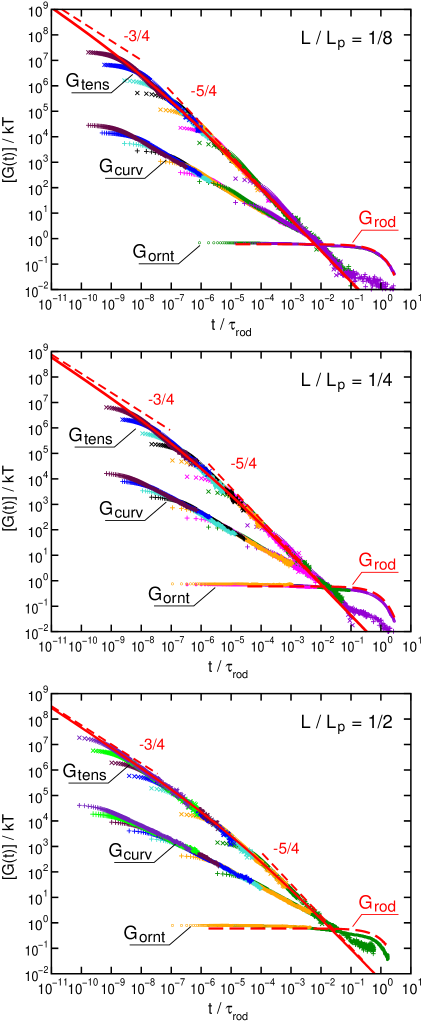
FIG. 1.: Simulation results for $[G_{\mathsf{tens}}(t)]$ (top curve in each plot, $\times$), $[G_{\mathsf{curv}}(t)]$ (middle curve, $+$), and $[G_{\mathsf{ornt}}(t)]$ (bottom curve, $\circ$) vs. $t/\tau_{\mathsf{rod}}$, with $\tau_{\mathsf{rod}}=\zeta_{b}N^{3}a^{2}/(72kT)$, for: $L/L_{p}=1/8$ and $N=8,16,22,32,46,64,90,128$ (top plot) $L/L_{p}=1/4$ and $N=8,16,22,32,46,64,90,128$ (middle plot), and $L/L_{p}=1/2$ and $N=16,32,64,90,128,180,256$ (bottom plot). In each plot, $[G_{\mathsf{ornt}}(t)]$ is shown only for a few small values of $N$. The long-dashed red line is the prediction $[G_{\mathsf{rod}}(t)]=\frac{3}{5}kTe^{-t/\tau_{\mathsf{rod}}}$ for rigid rods at $t>0$. Short-dashed red lines with slopes of $-3/4$ and $-5/4$ are asymptotes Eqs. (13) and (14). The solid red line is the predicted $[G_{\mathsf{tens}}(t)]$ obtained by Fourier transforming Eq. (12).

We now present a theory of the longitudinal dynamics of a rod-like chain that predicts the observed $t^{-5/4}$ decay of $[G_{\mathsf{tens}}(t)]$ at intermediate times for $L\ll L_{p}$. Our analysis resembles one given previously to describe longitudinal relaxation of entangled chains [5]. For rod-like chains, we may expand ${\bf r}(s,t)$ around a rod-like reference state as ${\bf r}(s,t)=r_{\parallel}(s,t){\bf n}(t)+{\bf h}(s,t)$, where ${\bf h}(s,t)$ satisfies ${\bf h}(s,t)\cdot{\bf n}(t)=0$, and ${\bf n}(t)$ is a unit vector that rotates with the flow like a non-Brownian rigid rod: $\dot{{\bf n}}={\bf P}\cdot\dot{\mbox{\boldmath$\gamma$}}\cdot{\bf n}$, where ${\bf P}\equiv{\bf I}-{\bf n}{\bf n}$. Linearizing Eq. (1) then yields longitudinal and transverse equations

$$\zeta\{\frac{\partial r_{\parallel}}{\partial t}-r_{\parallel}\dot{\mbox{\boldmath$\gamma$}}:{\bf n}{\bf n}\} = \frac{\partial{\cal T}}{\partial s}+\eta_{\parallel}$$ (7)

$$\zeta{\bf P}\cdot\{\frac{\partial{\bf h}}{\partial t}-\dot{\mbox{\boldmath$\gamma$}}\cdot{\bf h}\} = -\kappa\frac{\partial^{4}{\bf h}}{\partial s^{4}}+\frac{\partial}{\partial s}\left({\cal T}\frac{\partial{\bf h}}{\partial s}\right)+\mbox{\boldmath$\eta$}_{\perp}.$$ (8)

These equations are coupled by the tension ${\cal T}$, which is chosen to satisfy the constraint $|\frac{\partial{\bf r}}{\partial s}|^{2}=|\frac{\partial r_{\parallel}}{\partial s}|^{2}+|\frac{\partial{\bf h}}{\partial s}|^{2}=1$.

It is convenient to introduce a longitudinal strain field $\epsilon(s)\equiv\frac{\partial r_{\parallel}(s)}{\partial s}-\langle\frac{\partial r_{\parallel}}{\partial s}\rangle_{\mathsf{eq}}$, where $\langle\cdots\rangle_{\mathsf{eq}}$ denotes a thermal equilibrium average. Combining this definition with the constraint and expanding to lowest order in $|\partial{\bf h}/\partial s|^{2}$ yields an approximate expression of $\epsilon(s)$ in terms of ${\bf h}(s)$, $\epsilon(s)\simeq-\frac{1}{2}\left\{|\frac{\partial{\bf h}(s)}{\partial s}|^{2}-\langle|\frac{\partial{\bf h}(s)}{\partial s}|^{2}\rangle_{\mathsf{eq}}\right\}$. This expression for $\epsilon(s)$ and Eq. (8) were used in Refs [4, 5] to calculate the linear response of the spatial average strain $\langle\bar{\epsilon}(\omega)\rangle\equiv\int\!ds\langle\epsilon(s,\omega)\rangle/L$ to a spatially uniform oscillating tension ${\cal T}(\omega)$ at frequency $\omega$ (where functions of $\omega$ denote Fourier amplitudes), yielding an effective extension modulus $B(\omega)\equiv{\cal T}(\omega)/\langle\bar{\epsilon}(\omega)\rangle$ that is given by Eq. (3) at $\omega\gg\tau_{\perp}^{-1}$,[4, 5] and by a static value $B(0)\sim kTL_{p}^{2}/L^{3}$ at $\omega\ll\tau_{\perp}^{-1}$.[10]

A modified diffusion equation for the strain field may be obtained by taking the thermal average of Eq. (7), differentiating with respect to $s$, Fourier transforming with respect to $t$, and setting $\langle{\cal T}(s,\omega)\rangle=B(\omega)\langle\epsilon(s,\omega)\rangle$. This yields

$$\left(i\omega-\frac{B(\omega)}{\zeta}\frac{\partial^{2}}{\partial s^{2}}\right)\langle\epsilon(s,\omega)\rangle\simeq i\omega\mbox{\boldmath$\gamma$}(\omega):{\bf n}{\bf n}$$ (9)

where $B(\omega)/\zeta$ is an effective diffusivity and $\mbox{\boldmath$\gamma$}(\omega)$ is the amplitude of an oscillatory strain tensor. Hereafter ${\bf n}(t)$ is approximated by its time average over one period of oscillation. Eq. (9), with $\langle\epsilon(s,\omega)\rangle=0$ at the chain ends, has the solution

$$\langle\epsilon(s,\omega)\rangle=\left[1-\frac{\cosh(\lambda(\omega)(2\hat{s}-1))}{\cosh(\lambda(\omega))}\right]\mbox{\boldmath$\gamma$}(\omega):{\bf n}{\bf n}\quad,$$ (10)

where $\lambda(\omega)\equiv(i\omega\zeta L^{2}/4B(\omega))^{1/2}=(i\omega\tau_{\parallel}/2^{11})^{1/8}$.

The tension stress of rod-like chains subjected to an infinitesimal oscillatory strain $\mbox{\boldmath$\gamma$}(\omega)$ is given by

$$\mbox{\boldmath$\sigma$}_{\mathsf{tens}}(\omega)\simeq\int_{0}^{L}\!ds\;\langle{\cal T}(s,\omega)\ {\bf n}{\bf n}\rangle\quad.$$ (11)

where $\langle\cdots\rangle$ denotes an average over both weak fluctuations and overall rod orientations. Combining Eq. (11) with Eq. (10) for the strain along a rod of orientation ${\bf n}$ and averaging over random rod orientations yields a stress $\mbox{\boldmath$\sigma$}_{\mathsf{tens}}(\omega)=[G^{*}_{\mathsf{tens}}(\omega)][\mbox{\boldmath$\gamma$}(\omega)+\mbox{\boldmath$\gamma$}^{T}(\omega)]$, with a modulus

$$[G^{*}_{\mathsf{tens}}(\omega)]=\frac{1}{15}LB(\omega)\left[1-\frac{\tanh(\lambda(\omega))}{\lambda(\omega)}\right]\quad.$$ (12)

This prediction has the following limiting behaviors: At frequencies $\omega\gg\tau_{\parallel}^{-1}$, Eq. (12) reduces to the high-frequency asymptote $[G_{\mathsf{tens}}^{*}(\omega)]\simeq LB(\omega)/15$ found previously [4, 5]. Fourier transforming this asymptote yields a relaxation modulus

$$\lim_{t\ll\tau_{\parallel}}[G_{\mathsf{tens}}(t)]=C_{1}\frac{kTL}{L_{p}}\left(\frac{t}{\tau_{p}}\right)^{-3/4}\quad,$$ (13)

where $C_{1}=2^{3/4}/[15\Gamma(\frac{1}{4})]=0.0309$. At intermediate frequencies $\tau_{\parallel}^{-1}\gg\omega\gg\tau_{\perp}^{-1}$, where $\lambda(\omega)\ll 1$, expanding Eq. (12) in powers of $\lambda(\omega)$ yields a modulus $[G^{*}_{\mathsf{tens}}(\omega)]=i\omega\frac{\zeta L^{3}}{180}-\frac{kT}{1800\;2^{3/4}}(i\omega\tau_{\perp})^{5/4}+\cdots$, which includes a dominant contribution of order $i\omega$, whose prefactor is identical to that found for rigid rods, and a first correction proportional to $(i\omega)^{5/4}$. This yields a loss modulus $[G^{\prime\prime}(\omega)]\propto\omega$ (like rigid rods) but a storage modulus $[G^{\prime}(\omega)]\propto\omega^{5/4}$ (unlike rigid rods) at these frequencies. Upon transforming this intermediate asymptote, the term proportional to $i\omega$ yields an apparent $\delta$-function contribution to $[G(t)]$ (as for rigid rods), and so $[G_{\mathsf{tens}}(t)]$ is instead dominated at $\tau_{\parallel}\ll t\ll\tau_{\perp}$ by the transform of the term of proportional to $(i\omega)^{5/4}$, which yields

$$\lim_{\tau_{\parallel}\ll t\ll\tau_{\perp}}[G_{\mathsf{tens}}(t)]\simeq C_{2}kT\left(\frac{t}{\tau_{\perp}}\right)^{-5/4}\quad,$$ (14)

where $C_{2}=1/[2^{3/4}7200\Gamma(\frac{3}{4})]=0.0000674$. At $\omega\lesssim\tau_{\perp}^{-1}$ or $t\gtrsim\tau_{\perp}$, Eq. (3) for $B(\omega)$ becomes inapplicable, but $[G_{\mathsf{tens}}(t)]$ also becomes small compared to $[G_{\mathsf{ornt}}(t)]$.

The predictions of $[G_{\mathsf{tens}}(t)]$ shown in Fig. (1) were obtained by Fourier transforming Eq. (12) numerically. They agree with the simulation results for $[G_{\mathsf{tens}}(t)]$ at all $t\lesssim\tau_{\perp}$, and accurately describe not just the power law regimes, but the broad crossovers between them. Remarkably, the theory remains accurate for $L=L_{p}/2$, despite the assumption of a nearly straight chain.

Our derivation of Eq. (9) explicitly assumes a local proportionality of the tension and strain at each point on the chain, with $\langle\epsilon(s,\omega)\rangle=B^{-1}(\omega)\langle{\cal T}(s,\omega)\rangle$, rather than allowing for a spatially nonlocal response of the form $\langle\epsilon(s,\omega)\rangle=\int\!ds^{\prime}\;B^{-1}(s,s^{\prime},\omega)\langle{\cal T}(s^{\prime},\omega)\rangle$. To examine this approximation, we calculated the nonlocal compliance $B^{-1}(s,s^{\prime},\omega)$. We find that the range of nonlocality is of the order of the wavelength $\xi_{\perp}(\omega)=(\omega\zeta/kTL_{p})^{-1/4}$ of the bending mode with frequency $\omega$, and that the strain predicted by Eq. (9) varies slowly over lengths of order $\xi_{\perp}(\omega)$ for all $\omega\gtrsim\tau_{\perp}^{-1}$. This justifies our local compliance approximation for all $\omega\gtrsim\tau_{\perp}^{-1}$.

A conceptually simple, analytically solvable, and accurate model of the dominant contribution to $[G(t)]$ at times $t\lesssim\tau_{\perp}$, valid for all $L\lesssim L_{p}$, is thus obtained by treating the inextensible worm-like chain as an effectively extensible rod with a frequency-dependent longitudinal modulus given by Eq. (3). At later times, $[G(t)]$ is dominated by $[G_{\mathsf{ornt}}(t)]$, which mimics the behavior of a solution of rods. The simulations show that the curvature stress never dominates $[G(t)]$ in such solutions. A useful global approximation for $[G(t)]$ for rod-like chains may thus be obtained simply by replacing the $\delta$-function in Eq. (2) by our result for $[G_{\mathsf{tens}}(t)]$. Our results confirm that $[G(t)]$ initially decays as $t^{-3/4}$, but also show that, when $L\lesssim L_{p}$, this behavior is observable only below a time proportional to $\tau_{\parallel}$ that drops rapidly with decreasing $L/L_{p}$ to values inaccessible to either simulation or experiment. Therefore, measurements of the viscoelastic modulus of dilute solutions of rod-like chains at practically attainable high-frequencies may often probe either the $t^{-5/4}$ regime identified here, instead of the initial $t^{-3/4}$ regime, or the broad—but calculable—crossover between them.

Acknowledgements: This work was supported by NSF DMR-9973976 and Minnesota Supercomputing Institute.

REFERENCES

[1]
M. Doi and S. F. Edwards,
The Theory of Polymer Dynamics
(Oxford University Press, London, 1986).
[2] Slender body hydrodynamics for a rod-like polymer
predicts a mildly anisotropic friction tensor
,
with , with a logarithmic
dependence of on length scale. Here, we ignore both the
anisotropy and the weak scale-dependence for simplicity. See, e.g.,
G.K Batchelor, J. Fluid Mech.44, 419 (1970).
[3]
J. G. Kirkwood and P. L. Auer,
J. Chem. Phys.19, 281 (1951).
[4]
F. Gittes and F. C. MacKintosh,
Phys. Rev. E58, 1241 (1998).
[5]
D. C. Morse,
Phys. Rev. E58, 1237 (1998);
Macromolecules31, 7030, 7044 (1998).
[6]
R. Everaers, F. Julicher, A. Ajdari, and A. C. Maggs,
Phys. Rev. Lett.82, 3717 (1999).
[7]
P. S. Grassia and E. J. Hinch,
J. Fluid Mech.308, 255 (1996).
[8]
M. Fixman, J. Chem. Phys.69, 1527 (1978).
[9]
P. S. Doyle, E. S. G. Shaqfeh, and A. P. Gast,
J. Fluid Mech.334, 251 (1997).
[10]
F. C. MacKintosh, P. A. Janmey, J. Käs,
Phys. Rev. Lett.75, 4425 (1995).