Multi-component structure of nonlinear excitations
in systems with length-scale competition

Abstract

We investigate the properties of nonlinear excitations in different types of soliton bearing systems with long-range dispersive interaction. We show that length-scale competition in such systems universally results in a multi-component structure of nonlinear excitations and can lead to a new type of multistability: coexistence of different nonlinear excitations at the same value of the spectral parameter (i.e., velocity in the case of anharmonic lattices or frequency in nonlinear Schrödinger models).

1 Introduction

Physical systems with competition between discreteness, nonlinearity and dispersion are abundant in Nature. Examples are nonlinear charge and energy transport in biological macromolecules, elastic energy transfer in anharmonic chains, charge transport in hydrogen-bonded systems, coupled optical fibers, nonlinear photonic crystals, arrays of coupled Josephson junctions. Determination of their dynamical properties is of importance because of their wide applicability in various physical problems. In nonlinear systems with short-ranged (nearest-neighbor) dispersive interactions there are basically two types of nonlinear excitations. In the large dispersion (weak nonlinearity) limit when the discreteness of the lattice plays no essential role, the balance between nonlinearity and dispersion provides the existence of low-energy soliton-like excitations. The width of these excitations is large comparing with the lattice spacing, they freely propagate along the system without energy loss, their collisions are almost elastic. When the nonlinearity is strong (dispersion is weak) new nonlinear excitations, intrinsically localized modes, also called discrete breathers, may appear (see e.g. Ref. flach for a review). Their width is comparable with the lattice spacing, they are long-lived and robust.

The phenomenon of multistability, implying the coexistence of several stationary localized states having the same energy, appears in different contexts lst ; mal ; kladko ; ngfm ; gfnm ; mgm ; gmck ; gmcr ; mks ; jgcr ; jagcr ; gcrj ; kov . For the one-dimensional discrete nonlinear Schrödinger (NLS) equation with nearest-neighbor interactions (NNI) and arbitrary power of nonlinearity, multistability occurs when the power exceeds some critical value lst ; mal ; kladko .

Another mechanism of such multistability comes out for the systems with long-range dispersive interactions, where a new characteristic length scale appears: the radius of the dispersive interaction. As it was shown in Refs. ngfm ; gfnm ; mgm ; gmck ; gmcr ; mks the appearance of the new characteristic length scale brings into coexistence two stable stationary excitations one of which is a broad, continuum-like soliton and another is a narrow discrete excitation. This is a generic property of nonlinear systems with nonlocal dispersive interactions. The bistability occurs in such different systems as anharmonic chains with nonlocal interatomic interaction ngfm ; gfnm ; mgm , NLS models with long-range coupling gmck ; gmcr , and nonlinear waveguides in photonic crystals mks . In all these systems the bistability means that there is an interval of the energy $H$ where two stable nonlinear excitations (one of which is broad and another is intrinsically localized) coexist for each value of $H$. The greater the radius of the long-range interactions is, the more pronounced is the bistability phenomenon. A general mechanism for obtaining a controlled switching between bistable localized excitations was proposed in Refs. jgcr ; jagcr . Importantly, very similar types of excitations may appear in periodic nonlinear dielectric superlattices (two-dimensional nonlinear Kronig-Penney model gcrj ) where the nonlocality arises as a result of a reduction of the original two-dimensional problem to an effective one-dimensional description. Bistability in the spectrum of nonlinear localized excitations in magnets with a weak exchange interaction and strong magnetic anisotropy was found in Ref. kov .

Quite recently coexistence of different nonlinear excitations at the same value of the soliton velocity has been shown to take place in anharmonic chains with ultra-long-range interatomic interactions mgm00 . Specifically, it was shown that three different types of pulse solitons can coexist for each value of the pulse velocity in a certain velocity interval: one type is unstable but the two others can be stable. It should be emphasized the following intriguing aspect of the problem: in contrast to the previously discussed cases, now the bistability takes place at the same value of a spectral parameter (the soliton velocity in this system is mathematically the spectral parameter of a nonlinear eigenvalue problem). Therefore, the system being discussed provides us with the example of a new type of multistability whose physical consequences can be quite different from the multistability discussed above. Indeed, if such a new type of multistability can exist, for instance, for nonlinear waveguides in photonic crystals mks , then two different nonlinear modes with the same frequency of the light will coexist in a waveguide, which is practically more important than to have coexistence of nonlinear modes with the same energies but different frequencies.

The aim of the present paper is to demonstrate that the new type of multistability is a fundamental property of nonlinear systems with ultra-long-range dispersion. To this end we consider two additional (in comparison with Ref. mgm00 ) models: a discrete NLS equation with nonlocal dispersion and an anharmonic lattice with screened Coulomb interaction. We show that in both cases an ultra-long-range dispersive interaction results in a multi-valued dependence of the energy of stationary states on a spectral parameter (frequency in the case of the NLS equation and velocity in the case of the anharmonic lattice).

The outline of the paper is the following. In Sec. 2 we present the results of numerical simulations of stationary states in the discrete NLS model with a long-range dispersive interaction and in the anharmonic chain with a long-range dispersive interaction and cubic nearest-neighbor interaction. We discuss the appearance of a multi-valued dependence of the energy of the systems. In Sec. 3 we develop an analytical approach to the problem. We use a quasicontinuum approach which preserves both length scales that enter our problem. We show that the low-energy excitation can be considered as a compound state: a short-ranged breather-like component and a long-ranged component. Section 4 presents the concluding discussion.

2 Models and numerical results

We consider in parallel two nonlinear models which can bear pulse-like excitations: the Boussinesq equation model which describes the properties of anharmonic molecular chains and the nonlinear Schrödinger equation model which represents generic properties of a system of nonlinear oscillators.

2.1 Anharmonic chains with ultra-long-range dispersive interactions

Let us consider a chain of equally spaced particles of unit mass whose displacements from equilibrium are $u_{n}(t)$ and the equilibrium spacings are unity. The Hamiltonian of the system is given by

$$H=\sum_{n}\biggl{\{}\frac{1}{2}\Bigl{(}\frac{du_{n}}{dt}\Bigr{)}^{2}+V(u_{n+1}-u_{n})$$

$$+\frac{1}{2}\sum_{m>n}J_{m-n}(u_{m}-u_{n})^{2}\biggr{\}}\;,$$ (1)

with the anharmonic interaction

$$V(w)=w^{2}/2-w^{3}/3$$ (2)

between nearest neighbors and the harmonic long-range interaction (LRI)

$$J_{m-n}(\alpha,s)=J(\alpha,s)\,\frac{e^{-\alpha|m-n|}}{|m-n|^{s}}$$ (3)

between all particles of the chain. Here

$$J(\alpha,s)=J/F(e^{-\alpha},s)\;,$$ (4)

where

$$F(z,s)=\sum_{n=1}^{\infty}(z^{n}/n^{s})$$ (5)

is the so-called Joncqière’s function which properties are described in Ref. htf53 . $J$ characterizes the intensity of the LRI’s whereas $\alpha$ and $s$ determine their inverse radius. The coefficient $J(\alpha,s)$ is chosen in the form (4) to have the sum $\sum_{n}\,J_{n}(\alpha,s)$ independent of $\alpha$ and $s$. The parameters $\alpha$ and $s$ are introduced to cover different physical situations from the limit of nearest-neighbor interactions ($\alpha\gg 1$ or $s\gg 1$) to the limit of ultra-long-range interactions ($\alpha\ll 1$ and $s\leq 3$). The Hamiltonian (2.1) generates equations of motion of the form

$$\frac{d^{2}w_{n}}{dt^{2}} + 2W(w_{n})-W(w_{n+1})-W(w_{n-1})$$ (6)

$$+ \sum_{m\neq n}J_{m,n}(w_{n}-w_{m})=0\;,$$

where $w_{n}=u_{n+1}-u_{n}$ are relative displacements and $W(w)\equiv dV(w)/dw=w-w^{2}\,$. We use the quasicontinuum approach, regarding $n$ as a continuous variable: $n\rightarrow x,\,w_{n}(t)\rightarrow w(x,t)$, and using the operator identities

$$w(x+m,t) = \,e^{m\partial_{x}}w(x,t)\;,$$

$$Q(\alpha,s,\partial_{x}) \equiv \sum_{m=1}^{\infty}\frac{e^{-\alpha m}}{m^{s}}\,\frac{1-\cosh m\partial_{x}}{F\left(e^{-\alpha},s\right)}$$ (7)

$$= 1-\frac{F\left(e^{-\alpha-\partial_{x}},s\right)+F\left(e^{-\alpha+\partial_{x}},s\right)}{2\,F\left(e^{-\alpha},s\right)}\;.$$

In this approach the equation of motion (6) can be written in the pseudo-differential form

$$[\partial^{2}_{t}-JQ(\alpha,s,\partial_{x})]w(x,t)-4\sinh^{2}\biggl{(}\frac{\partial_{x}}{2}\biggr{)}W(w)=0\;,$$ (8)

where $\partial_{x}$ and $\partial_{t}$ are the derivatives with respect to $x$ and $t$, respectively. Eq. (8) can be called non-local Boussinesq equation.

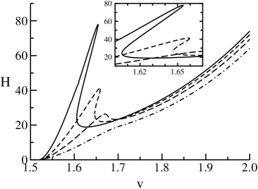
Figure 1: Energy of the pulse solitons versus velocity in the anharmonic lattice with Kac-Baker ($s=0$) long-range interaction found numerically for different values of $\alpha$ and $J$ (the value of $J$ was chosen to get constant $c=1.515$): $\alpha=0.05$ and $J=0.0016$ (full line); $\alpha=0.1$ and $J=0.0062$ (dashed line); $\alpha=0.17$ and $J=0.0172$ (long-dashed line); $\alpha=0.3$ and $J=0.05$ (dot-dashed line).

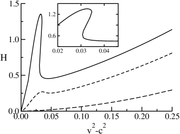
Figure 2: Energy of the pulse solitons versus velocity in the anharmonic lattice with screened Coulomb ($s=3$) interaction for $J=0.05$ and different values of $\alpha$: $\alpha=0.001$ (full line), $\alpha=0.005$ (dashed line), and $\alpha=\infty$ (long-dashed line).

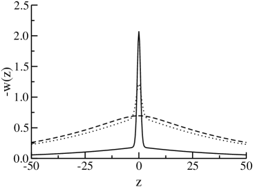
Figure 3: Shapes of the low-energy (full line), unstable intermediate-energy (dotted line), and high-energy (dashed line) pulse solitons which coexist at the same velocity $v=1.64$ in the anharmonic lattice with Kac-Baker ($s=0$) long-range interaction for $\alpha=0.05$ and $J=0.0016$ (see Fig. 1).

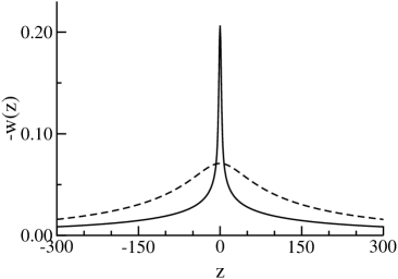
Figure 4: Shapes of the low-energy (full line) and high-energy (dashed line) pulse solitons which coexist at the same velocity $v^{2}-c^{2}=0.031$ in the anharmonic lattice with screened Coulomb ($s=3$) interaction for $J=0.05$ and $\alpha=0.001$ (see Fig. 2).

The energy (2.1) together with the momentum

$$P=\int_{-\infty}^{\infty}\Bigl{(}\frac{\partial u}{\partial t}\Bigr{)}\Bigl{(}\frac{\partial u}{\partial x}\Bigr{)}\,dx$$ (9)

are conserved quantities. We are interested in the stationary soliton solutions $w(x,t)\equiv w(x-vt)$ propagating with velocity $v$. Substituting $z=x-vt$ we can write Eq. (8) in the form

$$[v^{2}\partial^{2}_{z}-JQ(\alpha,s,\partial_{z})]w(z)-4\sinh^{2}\Bigl{(}\frac{\partial_{z}}{2}\Bigr{)}W(w)=0\;.$$ (10)

In this way we reduce our problem to a nonlinear eigenvalue problem with $v$ being a spectral parameter.

We consider two physically important cases: screened Coulomb interactions ($s=3$) and the Kac-Baker LRI’s ($s=0$). The speed of sound $c$ (which is an upper limit of the group velocity of linear waves), determined by the expression $c^{2}=1+JF\left(e^{-\alpha},s-2\right)/F\left(e^{-\alpha},s\right)$, grows indefinitely in both cases as $\alpha$ decreases. Using the Green’s function method mgm one can show that spatially localized stationary solutions (solitons) exist only for supersonic velocities $v>c$.

We have numerically integrated Eq. (10) using the method developed in Ref. mgm . Figures 1 and 2 show the dependence of the energy $H(v)$ (the dependence $P(v)$ has the same form) of the soliton solutions of Eq. (10) obtained for the Kac-Baker interaction ($s=0$) and screened Coulomb interaction ($s=3$), respectively. It is seen that the behavior in both cases is qualitatively the same. The soliton energy grows monotonically with the velocity in the case of large $\alpha$ (see, e.g., $\alpha=0.3$ in Fig. 1). In this case the soliton properties are qualitatively the same as in the limit of nearest-neighbor interactions (NNI’s) for which Eq. (8) reduces to the Boussinesq equation. It is well known that this equation has a sech-shaped soliton solution $w(z)=-1.5\,(v^{2}-c^{2})/\cosh^{2}(\sigma z)$, where $\sigma=\sqrt{3(v^{2}-c^{2})}$ is the inverse soliton width. As indicated above, the energy $H\sim(v^{2}-c^{2})^{3/2}$ of these solitons is a monotonic function of the velocity, which means that there is only one soliton solution for each given value of energy or velocity.

The situation changes when $\alpha<\alpha_{cr}$ (e.g., for the Kac-Baker interaction the critical value of inverse radius $\alpha_{cr}(J)$ is determined by Eq. (9) in Ref. mgm00 ). In this case, as was shown first in Ref. gfnm , the dependence $H(v)$ becomes non-monotonic (of $N$-shape, with a local maximum and a local minimum), so that there exist two branches of stable supersonic solitons: low-velocity and high-velocity solitons. These two soliton branches are separated by a gap (an interval of velocities where $H(v)$ decreases) with unstable soliton states. It is interesting that because of the non-monotonic dependence of $H(v)$ there exist low-velocity and high-velocity solitons of equal energy. Further increasing of the radius of the dispersive interaction (decreasing $\alpha$) leads to a $Z$-shape dependence of $H(v)$ (see Figures 1 and 2). In this case the gap which separated two above-mentioned soliton branches collapses; instead, there appears an interval of velocities where three soliton solutions with different energies and shapes (see Figures 3 and 4) coexist for each value of velocity. This phenomenon was first observed in Ref. mgm00 for the Kac-Baker dispersive interaction. Here we show that the same phenomenon takes place also in the case of the screened Coulomb interaction, but the radius of the interaction should be much larger: e.g., for the Coulomb dispersive interaction with the intensity $J=0.05$ the gap vanishes for $\alpha<0.0015$ while for the Kac-Baker interaction with the same intensity $J$ it happens for $\alpha<0.15$.

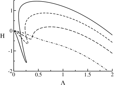
Figure 5: Energy $H$ of the stationary solitons versus nonlinear frequency $\Lambda$ in the NLS model with Kac-Baker ($s=0$) long-range interaction for different values of $\alpha$: $0.1$ (full line), $0.3$ (dashed line), $0.7$ (long-dashed line), and $\infty$ (dot-dashed line).

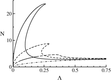
Figure 6: Number of quanta $N$ of the stationary solitons versus nonlinear frequency $\Lambda$ in the NLS model with Kac-Baker ($s=0$) long-range interaction for different values of $\alpha$: $0.1$ (full line), $0.3$ (dashed line), $0.7$ (long-dashed line), and $\infty$ (dot-dashed line).

2.2 Nonlinear Schrödinger model with ultra-long-range dispersive interaction

Let us now consider a system of coupled nonlinear oscillators which is described by the Hamiltonian

$$H=\frac{1}{2}\sum_{n}\Biggl{\{}\sum_{m\neq n}J_{n-m}(\alpha,s)|\psi_{n}-\psi_{m}|^{2}-|\psi_{n}|^{4}\Biggr{\}}\;,$$ (11)

where $n$ and $m$ are site indices, and $\psi_{n}$ is the excitation wave function. The first term in Eq. (11) describes a dispersive interaction between nonlinear oscillators. The second one represents a nonlinear interaction in the system. The case $\alpha=0$ in the dispersive interaction has been studied in detail in Ref. gmcr . Here we consider the dispersive interaction $J_{n-m}(\alpha,s)$ in the Kac-Baker form ($s=0$):

$$J_{n-m}=J(e^{\alpha}-1)\,e^{-\alpha|n-m|}\;.$$ (12)

It is important to investigate this type of the dispersive interaction because real physical systems which are described by the Hamiltonian (11) with the dispersive interaction given by Eq. (12) are not rare. For example, such type of excitation transfer may take place in systems where the dispersion curves of two elementary excitations are close or intersect and effective long-range transfer occurs at the cost of the coupling between excitations. This is the case for excitons and photons in semiconductors and molecular crystals. Dynamics of nonlinear photonic band-gap materials and periodic nonlinear dielectric superlattices is described gcrj by equations which are closely related to the equations which govern the dynamics of the discrete NLS model with the dispersive interaction in the Kac-Baker form (12). It was shown in Ref. gcrj that the radius of the effective dispersive interaction is proportional to the distance between nonlinear layers. Therefore one can easily tune the range of the dispersive interaction by preparing nonlinear lattices with different spacing between nonlinear layers.

In the Hamiltonian (11) $~{}\psi_{n}~{}$ and $~{}i\psi^{*}_{n}~{}$ are canonically conjugated variables and the equation of motion $~{}i\frac{d}{dt}\psi_{n}=\partial H/\partial\psi^{*}_{n}~{}$ has the form

$$i\frac{d\psi_{n}}{dt}+\sum_{m}\,J_{n-m}\,(\psi_{n-m}-\psi_{n})+|\psi_{n}|^{2}\psi_{n}=0\;.$$ (13)

The energy of the system $H$ together with the number of quanta

$$N=\sum_{n}\,|\psi_{n}|^{2}$$ (14)

are conserved quantities.

We study stationary states of the system

$$\psi_{n}(t)=\phi_{n}(\Lambda)\,e^{i\Lambda t}\;,$$ (15)

where $\Lambda$ is the nonlinear frequency and $\phi_{n}(\Lambda)$ is the amplitude at the $n$-th site. For small and intermediate radius ($\alpha^{-1}$) of the dispersive interaction the problem was studied in Refs. jgcr . It was shown that for $\alpha<1.7$ the NLS model exhibits bistability in the spectrum of nonlinear stationary states: for each value of $N$ in the interval $[N_{l}(\alpha),N_{u}(\alpha)]$ there exist three stationary states with frequencies $\Lambda_{1}(N)<\Lambda_{2}(N)<\Lambda_{3}(N)$. Since for discrete NLS equations a necessary and sufficient condition for linear stability of stationary states with a single maximum at a lattice site is $dN/d\Lambda\,>\,0$ (see, e.g., Ref. lst ), the low-frequency $\Lambda_{1}(N)$ and high-frequency $\Lambda_{3}(N)$ states, for which $dN/d\Lambda\,>\,0$, are stable (in what follows we shall refer to them as to the ‘low-frequency branch’ and ‘high-frequency branch’). There is an interval (‘gap’) of the nonlinear frequency $\Lambda$ which separates two branches of nonlinear excitations. Figures 5 and 6 show $H$ versus $\Lambda$ and $N$ versus $\Lambda$, respectively, obtained from direct numerical solution of Eq. (13) for different values of the inverse radius of dispersive interaction $\alpha$. It is seen that similar to the case of the nonlocal Boussinesq equation the gap decreases when the radius of the dispersive interaction increases and eventually it vanishes.

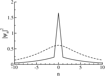
Figure 7: Shapes of the high-energy (full line) and low-energy (dashed line) stationary solitons which coexist at the same nonlinear frequency $\Lambda=0.25$ in the NLS model with Kac-Baker long-range interaction for $\alpha=0.3$ (see Fig. 5).

Comparing Figs. 1 and 2 obtained for the Boussinesq model with Fig. 5 obtained for the NLS model we see that several new but common for both models features arise as a consequence of the ultra-long-range dispersive interaction:

• The gap which separates two branches of stable stationary solutions decreases when the radius of the dispersive interaction $\alpha^{-1}$ increases.

• For small enough $\alpha$ (in the NLS model for $\alpha<0.57$) three different stationary states coexist for each value of spectral parameter (velocity $v$ in the case of the Boussinesq equation and nonlinear frequency $\Lambda$ in the NLS model). These three states are characterized by different values of the integrals of motion: the energy $H$ (in both models) and either the number of quanta $N$ (for the NLS equation) or the momentum $P$ (for the Boussinesq equation).

• The shapes of these states differ significantly (see Figs. 3–4 and 7). The high-energy state is broad and continuum-like while the low-energy states consist of two components, short-range and long-range ones. The width of the short-range component is of a few lattice spacing while the long-range component has tails which spread out a few tens of lattice constants.

• The state with an intermediate energy is always unstable while the stability of two other states depends on the radius of the dispersive interaction $\alpha^{-1}$. For example, in the case of the NLS equation for $\alpha\,>0.03$ the state which belongs to the high-frequency branch is unstable ($dN/d\Lambda\,<\,0$ for these $\alpha$). But this state becomes stable when $\alpha\,<\,0.03$.

3 Analytical approach

In our analytical approach we will be mostly concerned with the case of the NLS equation model because an analytical theory of multi-component solutions of the nonlocal Boussinesq equation is partially presented in Refs. gfnm ; mgm .

3.1 Nonlinear Schrödinger equation model

In the quasicontinuum approach, regarding $n$ as a continuous variable: $n\rightarrow x,\,\psi_{n}(t)\rightarrow\psi(x,t)$, Eq. (13) can be written as

$$i\partial_{t}\psi + \frac{J}{2}\,Q(\alpha,s=0,\partial_{x})\psi+|\psi|^{2}\psi=0\;,$$ (16)

where

$$Q(\alpha,s=0,\partial_{x})=(e^{\alpha}+1)\frac{4\sinh^{2}(\partial_{x}/2)}{\kappa^{2}-4\sinh^{2}(\partial_{x}/2)}$$ (17)

with $\kappa=2\sinh(\alpha/2)$ being a range parameter, is a linear pseudo-differential operator for the Kac-Baker dispersive interaction (12).

In order to obtain an analytic solution of the pseudo-differential equation (16) we use an approach akin to the previously proposed in Ref. rosenau : we multiply Eq. (16) by the operator $\frac{\partial^{2}_{x}}{4\sinh^{2}(\frac{\partial_{x}}{2})}$ and expand in a Taylor series this operator ($\frac{\partial^{2}_{x}}{4\sinh^{2}(\frac{\partial_{x}}{2})}\approx 1-\frac{1}{12}\partial^{2}_{x}$) as well as the operator $\sinh^{2}(\partial_{x}/2)$ in the denominator of the r.h.s. of Eq. (17). We stress that our modification of the standard continuum approximation is crucial in the preserving the second length scale that enters our problem. As a result we get a pseudo-differential equation

$$i\Bigl{(}1-\frac{\partial^{2}_{x}}{12}\Bigr{)}\partial_{t}\psi + \frac{J}{2}(e^{\alpha}+1)\frac{\partial^{2}_{x}}{\kappa^{2}-\partial^{2}_{x}}\psi+|\psi|^{2}\psi=0\;,$$ (18)

where the small term $\frac{1}{12}\partial^{2}_{x}|\psi|^{2}\psi$ was omitted.

Looking for stationary solutions

$$\psi=\sqrt{\frac{J}{2}(e^{\alpha}+1)}\,\Phi(x)\,e^{i\Lambda\tau}\;,$$ (19)

where $\tau=\frac{J}{2}(e^{\alpha}+1)t$, we can write Eq. (18) in the form

$$(\partial^{2}_{x}-s^{2}_{+})(\partial^{2}_{x}-s^{2}_{-})\Phi+\frac{12}{\Lambda}(\partial^{2}_{x}-\kappa^{2})\Phi^{3}=0\;,$$ (20)

with the parameters $s_{\pm}$ given by

$$s^{2}_{\pm} = \frac{1}{2}\Biggl{\{}\kappa^{2}+12\frac{\Lambda+1}{\Lambda}$$ (21)

$$\pm \sqrt{\left(\kappa^{2}+12\frac{\Lambda+1}{\Lambda}\right)^{2}-48\kappa^{2}}\Biggr{\}}\;.$$

In the limit of small $\alpha$

$$s^{2}_{-}\approx\frac{\Lambda\kappa^{2}}{\Lambda+1}\;,\qquad s^{2}_{+}\approx 12\frac{\Lambda+1}{\Lambda}\;.$$ (22)

For small nonlinear frequency $\Lambda$ we expect excitations with a width much larger than $s^{-1}_{+}$ so that only one scale $s^{-1}_{-}$ should be important. Since the characteristic width of the excitations of interest here is large as compared with $s^{-1}_{+}$, we can neglect the operator $\partial^{2}_{x}$ in the operator $(\partial^{2}_{x}-s^{2}_{+})$ and get

$$(\partial^{2}_{x}-s^{2}_{-})\Phi-\frac{1}{\Lambda+1}(\partial^{2}_{x}-\kappa^{2})\Phi^{3}=0\;.$$ (23)

This equation was investigated in Ref. gmck . It was shown that Eq. (23) has a soliton solution when the inequality $A=(\kappa^{2}/s^{2}_{-})\geq 9$ holds. As it is seen from Eq. (22) in the case of small $\alpha$ this inequality reduces to $\Lambda\,<\,1/8$. The number of quanta which corresponds to the solution of Eq. (23) has the form

$$N\equiv N_{<} = s_{+}^{2}\Lambda\frac{\kappa}{2\sqrt{A}}\Biggl{\{}1+\frac{A-9}{24}$$ (24)

$$\times \ln\left(\frac{(\sqrt{A}+1)(\sqrt{A}+3)}{(\sqrt{A}-1)(\sqrt{A}-3)}\right)\Biggr{\}}\;.$$

For large $\Lambda$, when both length-scales are important, we will seek a solution of Eq. (20) as the sum

$$\Phi=\sqrt{\frac{\Lambda}{12}}\left\{\phi_{S}(x)+\phi_{L}(x)\right\}\;,$$ (25)

where $\phi_{S}(x)$ is the short-range component and $\phi_{L}(x)$ is the long-range one. Here $\phi_{S}(x)$ will dominate in the center, while $\phi_{L}(x)$ in the tails.

Inserting Eq. (25) into Eq. (20) yields

$$(\partial^{2}_{x}-s^{2}_{-})\left\{(\partial^{2}_{x}-s^{2}_{+})(\phi_{S}+\phi_{L})+(\phi_{S}+\phi_{L})^{3}\right\}$$

$$-(\kappa^{2}-s^{2}_{-})(\phi_{S}+\phi_{L})^{3}=0\;.$$ (26)

Assuming that the function $\phi_{S}(x)$ satisfies the equation

$$(\partial^{2}_{x}-s_{+}^{2})\phi_{S}+3\phi_{L}(0)\phi_{S}^{2}+3\phi_{L}^{2}(x)\phi_{S}+\phi_{S}^{3}=0\;,$$ (27)

we obtain from Eq. (3.1) an equation for $\phi_{L}(x)$ in the form

$$(\partial^{2}_{x}-s^{2}_{-})(-s_{+}^{2}\phi_{L}+\phi_{L}^{3})+(s_{-}^{2}-\kappa^{2})\phi_{L}^{3}$$

$$=B\,(\kappa^{2}-s_{-}^{2})\,\delta(x)\;,$$ (28)

where

$$B = \int_{-\infty}^{\infty}dx\,\left\{\phi^{3}_{S}(x)+3\phi^{2}_{L}(x)\phi_{S}(x)+3\phi_{L}(x)\phi^{2}_{S}(x)\right\}$$ (29)

$$= s_{+}^{2}\int_{-\infty}^{\infty}dx\,\phi_{S}(x)\;.$$

To obtain Eq. (3.1) we took into account the big difference in the short-range scale $s_{+}^{-1}$ and the long-range scale $s_{-}^{-1}\,$. It permitted us to replace the product $~{}\phi_{L}(z)\phi_{S}(z)~{}$ by $~{}\phi_{L}(0)\phi_{S}(z)~{}$ in Eq. (27), to neglect the term $\partial^{2}_{z}\phi_{L}$ as compared with $s^{2}_{+}\phi_{L}$ in the l.h.s. of Eq. (3.1) and to replace the function $(\kappa^{2}-s^{2}_{-})\{\phi^{3}_{S}(x)+3\phi^{2}_{L}(x)\phi_{S}(x)+3\phi_{L}(x)\phi^{2}_{S}(x)\}$ by the r.h.s. of Eq. (3.1). Also, Eq. (27) was used in Eq. (29).

We obtain for the short-range component $\phi_{S}(x)$ the expression

$$\phi_{S}(x)=\frac{\sqrt{2}s_{+}(1-3a^{2})}{\sqrt{1-a^{2}}\cosh(\sqrt{1-3a^{2}}s_{+}x)+\sqrt{2}a}\;,$$ (30)

where $a=\phi_{L}(0)/s_{+}$ is the amplitude of the long-range component.

Eq. (3.1) on the half x-axis subject to the vanishing at infinity boundary conditions can be presented as

$$(s_{+}^{2} - 3\,\phi_{L}^{2})\,\partial_{x}\,\phi_{L}$$ (31)

$$= -\phi_{L}\,\sqrt{s_{+}^{4}\,s_{-}^{2}-s_{+}^{2}\,\frac{3\,s_{-}^{2}+\kappa^{2}}{2}\phi_{L}^{2}+\kappa^{2}\phi_{L}^{4}}$$

with the boundary condition at the origin in the form

$$-2\,\left(s_{+}^{2}-3\,\phi^{2}_{L}(0)\right)\,\partial_{x}\phi_{L}(+0) = (\kappa^{2}-s_{-}^{2})\,B\;.$$ (32)

Substituting Eqs. (29)–(31) into Eq. (32) we obtain that the amplitude $a$ of the long-range component is determined by the equation

$$\kappa=\frac{a\,R(a)\,A\sqrt{6}}{(A-1)\,\arccos\sqrt{2a^{2}/(1-a^{2})}}\;,$$ (33)

where $R(a)=\sqrt{A\,a^{4}-(A+3)\,a^{2}/2+1}\,$.

The number of quanta which corresponds to the solution (25) is determined by the expression

$$N\equiv N_{>} = (\Lambda+1)\Biggl{(}\frac{4}{s_{+}}\sqrt{1-3a^{2}}+\frac{6}{\kappa\sqrt{A}}\Biggl{\{}1-R(a)$$ (34)

$$+ \frac{A-9}{12\sqrt{A}}\ln\left|\frac{4R(a)+4Aa^{2}-A-3}{4\sqrt{A}-A-3}\right|\Biggr{\}}\Biggr{)}\;.$$

When $\kappa\,>\,\kappa_{b}$, where $\kappa_{b}\approx 0.63$ is the maximum value of the function in the r.h.s. of Eq. (33) for $A=9\,(\Lambda=1/8)$, Eq. (33) has only one solution in the interval $A<9\,(\Lambda>1/8)$. Inserting Eq. (33) into Eq. (34) and combining Eqs. (24) and (34) we obtain that the number of quanta $N$ as a function of $\Lambda$ has an $N$-type shape (see Fig. 6) with a finite gap which separates two branches of stable solitons. When $\kappa\,\leq\,\kappa_{b}$ the gap collapses and Eq. (33) has two solutions for $A>9$ ($\Lambda<1/8$). Taking into account that for $A>9$ ($\Lambda<1/8$) there exists also a low-frequency solution of Eq. (23), one can conclude that for $\kappa\,\leq\,\kappa_{b}$ there is an interval of $\Lambda$ where three stationary states correspond to each value of the nonlinear frequency. In this case the curve $N(\Lambda)$ has a $Z$-type shape (see Fig. 6). It is worth noticing that the bifurcation value for the inverse radius of the dispersive interaction $\alpha_{b}\approx 0.61$ ($2\sinh(\alpha_{b}/2)=\kappa_{b}$) obtained analytically is in a surprisingly good agreement with the value obtained from numerical simulations ($\alpha_{b}=0.57\pm 0.01$).

It is interesting also to note that when $\alpha\rightarrow 0$ the amplitude of the long-range component tends to zero while the short-range component in the low frequency limit becomes $\delta$-function like. This result is also in a good qualitative agreement with the results of numerical simulations (see Fig. 7).

3.2 Non-local Boussinesq equation model

Here we also restrict ourselves to the case when the dispersive interaction is of Kac-Baker type. In this case the quasicontinuum limit of the nonlocal Boussinesq equation (10) can be presented as follows gfnm

$$(\partial_{z}^{2}-\sigma_{+}^{2})(\partial_{z}^{2}-\sigma_{-}^{2})w(z)=\frac{12}{v^{2}}(\partial_{z}^{2}-\kappa^{2})w^{2}(z)\;,$$ (35)

where the parameters $\sigma_{\pm}$ play the same role as the parameters $s_{\pm}$ in the previous subsection. They are given by

$$\sigma^{2}_{\pm} = \frac{1}{2}\,\Biggl{\{}\kappa^{2}+12\frac{v^{2}-1}{v^{2}}$$ (36)

$$\pm \,\sqrt{\left(\kappa^{2}-12\frac{v^{2}-1}{v^{2}}\right)^{2}+48\kappa^{2}\frac{c^{2}-1}{v^{2}}}\Biggr{\}}\;,$$

where the speed of sound $c$ in the lattice with the Kac-Baker interaction is determined by the expression

$$c=\left[1+J\frac{{\rm e}^{-\alpha}+1}{({\rm e}^{-\alpha}-1)^{2}}\right]^{1/2}.$$ (37)

The parameter $\sigma_{+}$ is finite at all velocities $v\geq c$ and tends to $\sqrt{12}$ for $v\to\infty$. The parameter $\sigma_{-}$ vanishes at $v=c$ and tends to $\kappa$ for $v\to\infty$. One can find that in the travel-wave approach the Hamiltonian is determined by the expressions

$$H=vP-M(v)\;,$$ (38)

where $P$ is the canonical momentum and

$$M(v)=\frac{1}{6}\int_{-\infty}^{\infty}\,w^{3}(x)dx$$ (39)

is the nonlinear part of the Hamiltonian.

Near the speed of sound excitations have a width much larger than $\sigma^{-1}_{+}$ and can be described by Eq. (35) in the approximation $(\partial_{z}^{2}-\sigma_{+}^{2})w\approx-\sigma_{+}^{2}w$. In this approximation the soliton solutions exist in a finite interval of velocities, $c<v<v_{cr}\simeq\sqrt{(4c^{2}-1)/3}\,$. The explicit form of the low-velocity soliton in given in Ref. gfnm . Using this expression it is straightforward to obtain the energy of the soliton belonging to the low-velocity branch in the form

$$H_{<}=vP_{<}-M_{<}(v)\;,$$

$$P_{<}=\frac{\sigma_{+}^{4}v^{5}}{72{\cal A}^{2}\sigma_{-}}\left(\frac{{\cal A}-4}{3}I(w_{1})+2\right)\;,$$

$$M_{<}(v)=\frac{\sigma_{+}^{6}v^{6}}{93312\,{\cal A}^{3}}\biggl{(}{\cal A}^{2}-2{\cal A}+40$$

$$-\frac{({\cal A}-4)^{2}({\cal A}+5)}{3}I(w_{1})\biggr{)}\;,$$ (40)

with

$$I(w) = \int\limits_{0}^{w}\frac{1}{{\cal R}(x)}dx$$

$$= \frac{1}{\sqrt{{\cal A}}}\,\ln\left(\left|\frac{\sqrt{{\cal A}{\cal R}(w)}+{\cal A}w-({\cal A}+2)/3}{\sqrt{{\cal A}}-({\cal A}+2)/3}\right|\right)\;,$$

$${\cal R}(x) = \sqrt{{\cal A}x^{2}-\frac{2}{3}({\cal A}+2)x+1}\;,$$ (41)

where ${\cal A}\equiv(\kappa^{2}/\sigma_{-}^{2})>4$ in the velocity interval $c<v<v_{cr}$, and

$$w_{1}=\frac{1}{3{\cal A}}\left({\cal A}+2-\sqrt{({\cal A}-1)({\cal A}-4)}\right)$$ (42)

is the amplitude of the low-velocity soliton.

Far from the speed of sound we will use the same approach as in the previous subsection (see also Ref. gfnm ). We seek a solution of Eq. (10) as a sum

$$w(z)=w_{S}(z)+w_{L}(z)\;,$$ (43)

where $w_{S}(z)$ is the short-range component of the strain and $w_{L}(z)$ is the long-range one.

Assuming that the function $w_{S}(z)$ satisfies the equation

$$\partial^{2}_{z}w_{S}-\left(\sigma^{2}_{+}+\frac{24}{v^{2}}w_{L}(0)\right)w_{S}-\frac{12}{v^{2}}w^{2}_{S}=0\;,$$ (44)

we obtain from Eq. (35) an equation for $w_{L}(z)$ in the form

$$\partial^{2}_{z}(w_{L}+\frac{12}{v^{2}\sigma^{2}_{+}}w^{2}_{L})-\sigma_{-}^{2}w_{L}-\frac{12\kappa^{2}}{v^{2}\,\sigma_{+}^{2}}\,w^{2}_{L}$$

$$=-{\cal B}\,(\kappa^{2}-\sigma^{2}_{-})\,\delta(z)\;,$$ (45)

where

$${\cal B}=\int_{-\infty}^{\infty}dzw_{S}(z)\;.$$ (46)

To obtain Eqs. (44) and (3.2) we took into account the big difference in the short-range scale $\sigma_{+}^{-1}$ and the long-range one $\sigma_{-}^{-1}$ and proceeded in the same way as we did in the previous subsection. From Eq. (44) we get the short-range component $w_{S}$ in the form

$$w_{S}(z)=-\frac{1}{4}\sigma^{2}_{+}v^{2}(1-2\gamma)\,\mbox{sech}^{2}\left(\sqrt{1-2\gamma}\,\frac{\sigma_{+}z}{2}\right)\;,$$ (47)

where $\gamma=12\,|w_{L}(0)|\,/\,(v\sigma_{+})^{2}$ determines the amplitude of the long-range component. It can be found from the equation gfnm

$$3({\cal A}-1)\,\frac{\sigma_{-}}{\sigma_{+}}=\frac{\gamma{\cal R}(\gamma)}{\sqrt{1-2\gamma}}\;.$$ (48)

Note that there is a misprint in the corresponding equation of Ref. gfnm : one should omit $\bar{w}_{L}(0)$ (which plays the same role as $\gamma$ in this paper) in the nominator of the fraction in the l.h.s. of Eq. (A.19).

Using Eqs. (47), (43), and (48) one can obtain that the energy of the compound soliton (43), i.e. the soliton which belongs to the high-velocity branch, can be presented in the form

$$H_{>}=vP_{>}-M_{>}(v)\;,$$ (49)

where

$$P_{>} = \frac{\sigma_{+}^{4}v^{5}}{72}\biggl{(}\frac{3}{\sigma_{+}}\sqrt{1-2\gamma}$$ (50)

$$+ \frac{1}{{\cal A}^{2}\sigma_{-}}\left[2+\frac{{\cal A}-4}{3}I(\gamma)-(2+{\cal A}\gamma){\cal R}(\gamma)\right]\biggr{)}$$

is the canonical momentum of the compound soliton and

$$M_{>}(v)=\frac{1}{2880}\sigma_{+}^{5}v^{6}\sqrt{1-2\gamma}\left(3\gamma^{2}-3\gamma+2\right)$$

$$+\frac{\sigma_{+}^{6}v^{6}}{93320{\cal A}^{3}}\biggl{(}({\cal A}^{2}-2{\cal A}+40)(1-{\cal R}(\gamma))$$

$$-{\cal A}({\cal A}+20)\gamma{\cal R}(\gamma)-\frac{({\cal A}-4)^{2}({\cal A}+5)}{3}I(\gamma)\biggr{)}$$ (51)

is the corresponding nonlinear part.

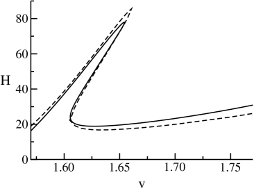
Figure 8: Energy of the pulse solitons versus velocity in the anharmonic lattice with Kac-Baker ($s=0$) long-range interaction calculated numerically (full line) and analytically (dashed line) for $\alpha=0.05$ and $J=0.0016$.

In the velocity interval $v\,>\,v_{c}$ (${\cal A}\,<\,4$) Eq. (48) for all values of the inverse radius $\alpha$ has a solution which tends to zero when $v\rightarrow\infty$. There is an one-to-one correspondence between the velocity of soliton and its energy. But when

$$\frac{\kappa^{2}(4c^{2}-1)}{c^{2}-1}\leq\frac{64}{729}$$ (52)

Eq. (48) has also two solutions in the interval $v\,<\,v_{c}~{}({\cal A}\,>\,4)~{}$. In other words under the condition (52), which taking into account the explicit form of the speed of sound (37), can be written as

$$J\geq\frac{3\alpha^{4}}{8(\alpha_{o}^{2}-\alpha^{2})}$$ (53)

with $\alpha_{o}\approx 0.16$, there exist three stationary pulse solitons with different energy for each value of the velocity and the function $H(v)$ has a characteristic $Z$-shape (see Fig. 1). Comparison the dependence $H(v)$ obtained analytically from Eqs. (3.2), (49)-(3.2) with the dependence obtained numerically shows a good agreement between these two approaches (see Fig. 8). The function (53) also describes very well the boundary which separates the area where $H(v)$ has a $N$-shape and a $Z$-shape (see Fig. 3 in Ref. mgm ).

4 Conclusion

We investigated the effect of length scale competition in two systems which can bear pulse-like nonlinear excitations: a chain of coupled nonlinear oscillators (nonlinear Schrödinger model) and an anharmonic chain with cubic nearest-neighbor interaction. Two types of dispersive interactions were studied: the Kac-Baker interaction and screened Coulomb interaction. We have shown that the existence of two competing length scales: the radius of the dispersive interaction and lattice spacing provides the existence of two types of pulse solitons one of which is broad, continuum-like and uni-component, and another is narrow, discrete-like and has a compound structure. It consists of two components: short-ranged breather-like component which dominates near the center of the excitation and long-ranged component which contributes mainly to the tails of the excitation. These two stable solitons are separated by gap: an interval of spectral parameter (velocity in the case of Boussinesq equation and frequency in the case of Nonlinear Schrödinger equation) where there are no stable stationary excitations. We show that the gap decreases when the radius of the dispersive interaction increases and it closes when the radius of the dispersive interaction exceeds some critical value. In contrast to systems with short-range and moderate-range dispersive interactions, where there is unambiguous correspondence between the velocity (frequency in the NLS equation) of the soliton and its energy, in systems where the length scales differ significantly (ultra-long-range interaction) there is an interval where three different states with different energies (momentum, number of quanta, etc.) correspond to each value of the spectral parameter. This is a generic property of all systems with competing length scales and is due to the compound structure of excitations.

References

- (1) S. Flach and C.R. Willis, Phys. Rep. 295, 181 (1998).
- (2) E.W. Laedke, K.H. Spatschek, and S.K. Turitsyn, Phys. Rev. Lett. 73, 1055 (1994); E.W. Laedke, O. Kluth, K.H. Spatschek, Phys. Rev. E 54, 4299 (1996).
- (3) B.A. Malomed and M.I. Weinstein, Phys. Lett. A 220, 91 (1996).
- (4) S. Flach, K. Kladko, and R.S. MacKay, Phys. Rev. Lett. 78, 1207 (1997).
- (5) A. Neuper, Yu. Gaididei, N. Flytzanis, and F.G. Mertens, Phys. Lett. A 190, 165 (1994).
- (6) Yu. Gaididei, N. Flytzanis, A. Neuper, and F.G. Mertens, Phys. Rev. Lett. 75, 2240 (1995); Physica D 107, 83 (1997).
- (7) S.F. Mingaleev, Yu.B. Gaididei, and F.G. Mertens, Phys. Rev. E 58, 3833 (1998).
- (8) Yu.B. Gaididei, S.F. Mingaleev, P.L. Christiansen, and K.Ø. Rasmussen, Phys. Lett. A 222, 152 (1996).
- (9) Yu.B. Gaididei, S.F. Mingaleev, P.L. Christiansen, and K.Ø. Rasmussen, Phys. Rev. E 55, 6141 (1997).
- (10) S.F. Mingaleev, Yu.S. Kivshar, and R.A. Sammut, Phys. Rev. E 62, 5777 (2000).
- (11) M. Johansson, Yu. B. Gaididei, P.L. Christiansen, and K.Ø. Rasmussen, Phys. Rev. E 57, 4739 (1998).
- (12) M. Johansson, S. Aubry, Yu.B. Gaididei, P.L. Christiansen, and K.Ø. Rasmussen, Physica D 119, 115 (1998).
- (13) Yu.B. Gaididei, P.L. Christiansen, K.Ø. Rasmussen, and M. Johansson, Phys. Rev. B 55, R13365 (1997).
- (14) M.V. Gvozdikova and A.S. Kovalev, Low Temp. Phys. 24, 808 (1998) [Fiz. Nizk. Temp. 24, 1077 (1998)].
- (15) S.F. Mingaleev, Yu.B. Gaididei, and F.G. Mertens, Phys. Rev. E 61, R1044 (2000).
- (16) W. Magnus, F. Oberhettinger and R.P. Soni, Formulas and Theorems for the Special Functions of Mathematical Physics (Springer-Verlag, Berlin – Heidelberg – New York, 1966).
- (17) P. Rosenau, Phys. Lett. A 118, 222 (1986).