Theory and Applications of X-ray Standing Waves in Real Crystals

Abstract

Theoretical aspects of x-ray standing wave method for investigation of the real structure of crystals are considered in this review paper. Starting from the general approach of the secondary radiation yield from deformed crystals this theory is applied to different concreate cases. Various models of deformed crystals like: bicrystal model, multilayer model, crystals with extended deformation field are considered in detailes. Peculiarities of x-ray standing wave behavior in different scattering geometries (Bragg, Laue) are analysed in detailes. New possibilities to solve the phase problem with x-ray standing wave method are discussed in the review. General theoretical approaches are illustrated with a big number of experimental results.

A.V. Shubnikov Institute of Crystallography, Russian Academy of Science, Leninsky pr. 59, 117333 Moscow, Russia

CONTENTS

1. Introduction

2. X-ray dynamical diffraction in real crystals

2.1 Takagi-Taupin equations

2.2 Susceptibilities

3. Theory of x-ray standing waves in a real crystal (general approach)

4. XSW in a perfect crystal

4.1 XSW with a big and small depth of yield (extinction effect)

4.2 Multicomponent crystals

4.3 Crystals with an amorphous surface layer

5. Bicrystal model (Bragg geometry)

5.1 Theory

5.2 Experiment

6. XSW in Laue geometry

6.1 Theory

6.2 Experiment

7. Model of a multilayer crystal

7.1 Theory

7.2 Applications

8. Crystals with an extended deformation field

8.1 Crystals with the uniform strain gradient. Bent crystals

8.2 Vibrating crystals

9. Phase problem

10. Conclusions

11. Appendix

Secondary radiation yield from a multilayer crystal (analytical approach)

1 Introduction

A new field in the physics of x-ray diffraction has appeared and successfully developed during last 30 years. It is based on studying and using x-ray standing waves (XSW) that are formed in a perfect crystal under conditions of dynamical diffraction. Apart from general physical interest involving the enormously sharp change in the interaction of x-rays with atoms in the crystal and on its surface, this field, as has now become clear, is highly promising for analyzing the structure of crystals and its adsorbates at the atomic level.

Actually a standing wave that has the same period as the crystal lattice is extremely sensitive to the slightest deviation of the atomic planes (or individual atoms) from their correct position in the perfect crystal (or on its surface). Thus XSW method is particularly useful in its application for structural analysis. For this technique, an x-ray interference field (XIF) is produced by the superposition of, typically, two plane x-ray waves. In this case we have the following expression for the amplitude of the electric field in the crystal:

$$\mathbf{E}(\mathbf{r})=\mathbf{E}_{0}e^{i\mathbf{k}_{0}\mathbf{r}}+\mathbf{E}_{h}e^{i\mathbf{k}_{h}\mathbf{r}},$$ (1)

where $\mathbf{k}_{0}$ is an incident wave vector, $\mathbf{k}_{h}=\mathbf{k}_{0}+\mathbf{h,}$ and $\mathbf{h}$ is the reciprocal lattice vector multiplied by $2\pi.$ The field intensity is determined by the square of the modulus of the amplitude $\mathbf{E}(\mathbf{r})$ and is equal to

$$I(\mathbf{r})=|\mathbf{E}_{0}|^{2}\left[1+\frac{|\mathbf{E}_{h}|^{2}}{|\mathbf{E}_{0}|^{2}}+2\frac{|\mathbf{E}_{h}|}{|\mathbf{E}_{0}|}\cos\left(\mathbf{hr}+\alpha(\theta)\right)\right],$$ (2)

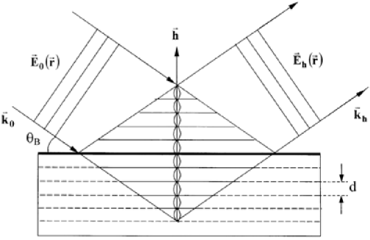
Figure 1: Interference x-ray standing wave field as a result of coherent superposition of the incident $\mathbf{E}_{0}(\mathbf{r})$ and diffracted $\mathbf{E}_{h}(\mathbf{r})$ plane waves with the periodicity $d=2\pi/|\mathbf{h}|$.

where $\alpha(\theta)$ is the phase of the ratio $\mathbf{E}_{h}/\mathbf{E}_{0}$. The spatial position of the planar wave field is determined by the phase $\alpha(\theta)$ between the two (electric) field amplitudes. Generated via Bragg reflection, employing a diffraction vector $\mathbf{h}$, the x-ray standing wave exists within the overlap region of the incident and reflected x-ray wave (Fig.1) and the phase $\alpha(\theta)$ and thus the position of the wave field is a function of the angle $\theta$ measured from exact Bragg angle, varying by half a diffraction plane spacing within the total reflection range. Thus, atomic positions can be scanned by the XIF and exactly determined if the yield of the element specific photoelectrons or x-ray fluorescence photons is recorded as a function of the glancing angle.

Structural analysis by the XSW technique represents actually a Fourier analysis but, in contrast to diffraction techniques, the atomic distribution of an elemental sublattice is sampled. The two important parameters which are determined by an XSW measurement are called coherent fraction ($F_{c}^{h}$) and coherent position ($P_{c}^{h}$) and represent the $\mathbf{h}$–th amplitude and phase, respectively, of the Fourier decomposition of the distribution of atoms under consideration. The XSW method is particularly powerful for the analysis of the structure of adsorbates on crystalline substrates since the position of the adsorbate atom within the surface unit cell can be determined with high accuracy for low adsorbate coverages. In case several elements are present on the surface, $F_{c}^{h}$ and $P_{c}^{h}$ can be obtained for each elemental sublattice within one XSW measurement.

An effect involving the existence of a standing wave and the variation of the total field at the atoms of the crystal lattice has been known for a long time (see for example [1, 2, 3]). However in the conditions of a classical x-ray diffraction experiment, when the intensity of the reflected and transmitted waves is measured separately it is manifested very weakly. This is mainly due to the fact, that the cross sections of the inelastic scattering channels are considerably smaller, than the cross section of elastic scattering [4]. The standing wave in the crystal reveals itself in a traditional x-ray diffraction experiment only in the form of an anomalous angular dependence of the absorption (the anomalous transmission effect in the Laue case as discovered by Borrmann [5]) and also the weak asymmetry of the reflectivity curve in the Bragg case [1, 2, 3].

Batterman [6] was the first who made an attempt to see the standing wave and its behavior by measuring the $GeK_{\alpha}$ fluorescence emitted by crystal atoms. Despite expectations, the measured curve has the angular dependence similar to the inverted reflectivity curve of the x-rays. The structure of the wave field manifested itself very weakly only at the edges of the total reflection region. It was soon understood [7], that this behavior was due to the fact, that the depth of yield $L_{yi}$ of the fluorescence radiation exceeds by far the penetration depth of x-rays in the crystal. This penetration depth while the dynamical diffraction of x-rays is of the order of extinction length $L_{ex}$. As a result all the radiation absorbed in the crystal gives rise to a fluorescence signal. Its amount, following the law of conservation of energy is equal to $1-P_{R}(\theta)$, where $P_{R}(\theta)$ is the reflectivity curve. The secondary radiation (SR) yield is proportional to the wave field intensity (2) at the atoms only if the condition ($L_{yi}<<L_{ex}$) is fulfilled. Later there were proposed methods for revealing the structure of the wave field by measuring the fluorescence yield from the impurity atoms introduced in the lattice of the crystal matrix at a very small depth [8] or measuring the fluorescence signal at grazing exit angles [7]. Evidently the condition $L_{yi}<L_{ex}$ is satisfied in this cases. Moreover, for a monolayer of atoms absorbed on the surface of crystal this condition for the escape depth of the SR is surely satisfied.

The above mentioned problem does not exist in measurements of the photoelectron emission since electrons escape from a thin subsurface layer with a thickness of fractions of a micrometer. Already in the first works on the measurement of the photoelectron emission, carried out in the former Soviet Union in the early 70’s [9, 10], the dispersion like angular dependence corresponding to the behavior of an x-ray standing wave (2) was observed. What was understood from the very beginning that this angular dependence of the photoelectron yield curve contain essential information about the structure of the surface layers. Later this field of research was developing intensively in several scientific centers of the former Soviet Union (see for details review paper [11] and a book [12]).

Already in the middle sixties first attempts to measure different secondary processes were made. For example measurements of thermal diffuse and Compton scattering while the existence of the standing wave in the crystal were reported [13, 14, 15] (see also later experimental paper [16]). The angular dependence of the photoelectric current in the silicon crystal with $p-n$ junction while the dynamical scattering of x-rays was measured [17, 18].

During last decade, due to the availability of the synchrotron radiation facilities of last generation (ESRF, APS, Spring-8) XSW method has become a useful and even in some cases a routine tool for investigating the surface of the crystals and the structure of the adsorbates. Most of the results obtained up to the beginning of 90-th, especially applications of XSW technique to surface analysis were summarized in a review paper [19], an overview of the method was also given in a number of papers [20, 21, 22, 23]. However one of the important field of applications of the XSW method for investigation of the structure of the real crystals (containing different type of defects, implanted crystals, epilayers on the surface of the perfect crystals, geterostructures etc.) has not been reviewed up to now. Previous review on this subject [11] was written nearly fifteen years ago (see also the book [12]) and a big number of new results are not summarized until now. At the same time still it is a big interest to the foundations of the theory of XSW in real crystals (see for example recent paper [24]). In our work we are planning to fill this gap. Theoretical approach is illustrated by the experimental results obtained in the Laboratory of Coherent Optics and Synchrotron Radiation of the Institute of Crystallography RAS. Due to a limited size of this manuscript we have no possibility to give a detailed consideration of all results obtained in the field of XSW method in different research centers all over the world. Some of them are just mentioned or even not mentioned, but this, surely, does not mean that they are not relevant to the subject. This can be a special subject of another review paper.

If XSW method in perfect crystals is based on the dynamical theory of x-ray diffraction (see for e.g. books and reviews [1, 2, 3, 25, 26]) for the description of the fields and the yield of the secondary radiation from the real crystals it is most effective to use Takagi-Taupin theory [27, 28, 29] of the propagation of x-rays in the deformed crystals. For convenience of the reader we start Chapter II with formulation of the main results of this theory that will be used in the following parts of the work. In the end of the same Chapter for the same reason we give the main relationships for the description of the real and imaginary part of the susceptibilities in crystals in x-ray wavelength region. For a recent review of the dynamical theory of x-ray diffraction in a perfect and deformed crystals see also [30, 31]. Chapter III gives a general mathematical formalism for calculating the secondary radiation yield in a real crystal. This chapter is based on the results of the paper [32] and represents the theoretical foundation for the remainder of this review paper. Next Chapter IV is devoted to the theory of XSW in the case of perfect crystals. Peculiarities of the secondary radiation yield with the big and small depth of yield of the secondary radiation are discussed, in the next subsection fluorescence and photoemission yield from the crystals containing different type of atoms is analysed and in the end of the chapter crystals with amorphous surface layer are discussed. Chapter V is devoted to very important and often realized case of deformed crystal, that can be approximated in the frame of bicrystal model. In the first subsection theory of the secondary radiation yield from such a model crystal in the Bragg geometry is presented and in the following subsection it is illustrated by a numerous examples. In the next Chapter VI Laue geometry is considered, peculiarities of x-ray standing wave behavior in this geometry are discussed and illustrated by examples. In Chapter VII the bicrystal model is generalized to the case of a multilayer model of the deformed layer and a secondary radiation yield from such system is analyzed theoretically and with its applications to the study of implanted crystals. Secondary radiation yield from the crystals with extended deformation yield are considered in Chapter VIII. There is given a detailed description of the wave fields in the case of the crystals with the uniform strain gradient, which includes the case of bent crystals and as a special case vibrating crystals. Next Chapter IX describes one of the important applications of the XSW analysis: the possibility to solve a phase problem while x-ray scattering from deformed crystal. This approach opens the possibility to determine uniquely the structure of the surface layer directly from the scattering experiment. Last Section X presents a summary and an outlook for the future applications of the XSW method in real crystals.

2 X-ray dynamical diffraction in real crystals

2.1 Takagi-Taupin equations

Directly from the Maxwell’s equations for the electric field vector $\mathbf{E}(\mathbf{r},\omega)$ ($\omega$ is the frequency of the incident wave) inside a crystal we can obtain the following wave propagation equation,

$$(\mathbf{\Delta+k^{2}})\mathbf{E}(\mathbf{r},\omega)-graddiv\mathbf{E}(\mathbf{r},\omega)=-k^{2}\frac{4\pi i}{\omega}\mathbf{j}(\mathbf{r},\omega),$$ (3)

where $k=|\mathbf{k}|=\omega/c$ is the magnitude of the wave vector ($c$ is the velocity of light), $\mathbf{j}(\mathbf{r},\omega)$ is the current density induced by the electromagnetic field. This current in the case of linear electromagnetic wave theory is, in fact, a linear function of $\mathbf{E}(\mathbf{r},\omega)$,

$$j_{i}(\mathbf{r},\omega)=\int d\mathbf{r}^{\prime}\sigma_{ik}(\mathbf{r},\mathbf{r}^{\prime},\omega)E_{k}(\mathbf{r}^{\prime},\omega),$$ (4)

where $\sigma_{ik}(\mathbf{r},\mathbf{r}^{\prime},\omega)$ is the nonlocal tensor of the conductivity of the crystal. In general case equation (4) describes non-local coupling between $\mathbf{j}(\mathbf{r},\omega)$ and $\mathbf{E}(\mathbf{r},\omega)$. It takes into account all possible interactions (such as elastic Thompson scattering, photoelectric absorption, Compton scattering and an inelastic scattering on thermal phonons) between the electromagnetic wave and the crystal [33]. The main contribution to $\sigma_{ik}(\mathbf{r},\mathbf{r}^{\prime},\omega)$ is connected with elastic Thompson scattering and has a strictly local character (the same is valid for the main inelastic process, that is photoelectron absorption in the dipole approximation) so we can present the tensor of the conductivity in the following way:

$$\sigma_{ik}(\mathbf{r},\mathbf{r}^{\prime},\omega)=\sigma(\mathbf{r},\omega)\delta_{ik}\delta(\mathbf{r}-\mathbf{r}^{\prime}),$$ (5)

where $\delta_{ik}$ is the Kroneker symbol and $\delta(\mathbf{r}-\mathbf{r}^{\prime})$ is the Dirac $\delta-$function.

For further consideration, if it is not specially noted, we will assume local coupling (5). According to (5), the right hand side of equation (3) takes the form,

$$\frac{4\pi i}{\omega}\mathbf{j(r,}\omega\mathbf{)}=\chi\mathbf{(r,}\omega\mathbf{)E(r,}\omega\mathbf{),}$$ (6)

where $\chi\mathbf{(r,}\omega\mathbf{)=(}4\pi i/\omega)\sigma(\mathbf{r},\omega)$ is the crystal susceptibility, related with the permittivity $\varepsilon\mathbf{(r,}\omega\mathbf{)}$ of the crystal by usual equation: $\varepsilon\mathbf{(r,}\omega\mathbf{)=}1+\chi\mathbf{(r,}\omega\mathbf{)}$ .

In a perfect (ideal) crystal susceptibility $\chi\mathbf{(r)}$ is a periodic function with the period of the crystal lattice $\chi\mathbf{(r)=}\chi\mathbf{(r+a),a}$ is the translation vector. It can be therefore expanded as a Fourier series,

$$\chi^{(id)}\mathbf{(r)=}\sum\limits_{h}\chi_{h}^{(id)}\exp(i\mathbf{hr}),$$ (7)

where $\mathbf{h=}2\pi\mathbf{H,}$ $\mathbf{H}$ is the reciprocal lattice vector.

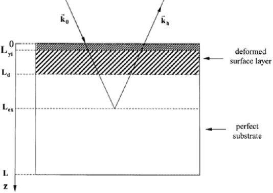
Figure 2: Crystal of thickness $L$, with the deformed surface layer of thickness $L_{d}$. While the Bragg diffraction x-rays penetrate into the crystal on the depths of the order of $L_{ex}$. The depth of the SR yield is determined by the parameter $L_{yi}$. It is shown the situation, when the condition $L_{yi}<<L_{d}<<L_{ex}$ is satisfied.

We shall assume now, that some part of a crystal lattice (in most of applications it is a thin surface part of the crystal (see Fig.2)) is weakly deformed due to epitaxial growth, implantation or some other type of deformation or defects. It is convenient to describe this weak deformation field of a crystal lattice by two functions. The first one is the deformation vector $\mathbf{u}(\mathbf{r})$, which determines the displacements of atoms in a crystal from the position of perfect lattice and the second one is the static Debye-Waller factor $e^{-W(r)}$ which takes into account the random displacements of the atoms from the equilibrium positions in the $\mathbf{h}$ direction.

In the case of weak deformations, that means that relative displacements are small on interatomic distances,

$$\left|\frac{\partial u^{i}}{\partial x_{k}}\right|<<1,$$ (8)

the susceptibility of the crystal $\chi(\mathbf{r})$ is defined from that of a perfect one according to relation [28],

$$\chi(\mathbf{r})=\chi^{(id)}(\bf{r-u}(\bf{r})).$$ (9)

The Fourier components of the susceptibility in the weakly deformed crystal (now depending from the coordinate $\mathbf{r}$) can be defined according to Eq. (9) as

$$\chi_{h}(\mathbf{r})=\chi_{h}^{(id)}\exp\left[-i\mathbf{hu}(\mathbf{r})\right]e^{-W(r)}.$$ (10)

We shall look for the solution of equation (3) in the form of the expansion analogous to the Bloch waves,

$$\mathbf{E(\bf{r}})=\sum\limits_{h}\mathbf{E}_{h}(\mathbf{r})\exp(i\mathbf{k}_{h}\mathbf{r}),$$ (11)

$$\mathbf{k}_{h}=\mathbf{k}_{0}+\mathbf{h}.$$ (12)

Here $\mathbf{k}_{0}$ and $\mathbf{k}_{h}$ are the incident and diffracted wave vectors and the sum has to be taken over all reciprocal lattice vectors $\mathbf{h}$. In the case of the weakly deformed crystal, when inequality (8) is satisfied the amplitudes $\mathbf{E}_{h}(\mathbf{r})$ in the expansion (11) are slowly varying functions of coordinate (on the contrary to the Bloch waves in a perfect crystal, when they does not depend on $\mathbf{r}$). This amplitudes vary significantly on the distances much bigger, then the X-ray wavelengths (of the order of extinction length $L_{ex}$ that will be defined later). Therefore, if we neglect the second derivatives of $\mathbf{E}_{h}(\mathbf{r})$ we can obtain from (3) the following set of equations,

$$\frac{\partial}{\partial\mathbf{s}_{h}}\mathbf{E}_{h}(\mathbf{r})=\frac{ik}{2}\sum\limits_{h^{\prime}}\left[\chi_{hh^{\prime}}(\mathbf{r})-\alpha_{h^{\prime}}\delta_{hh^{\prime}}\right]\mathbf{E}_{h^{\prime}}(\mathbf{r}),$$ (13)

where

$$\alpha_{h}=\frac{\mathbf{k}_{h}^{2}-\mathbf{k}_{0}^{2}}{\mathbf{k}_{0}^{2}};\frac{\partial}{\partial\mathbf{s}_{h}}=(\mathbf{s}_{h}\bigtriangledown);\mathbf{s}_{h}=\frac{\mathbf{k}_{h}}{\left|\mathbf{k}_{h}\right|},$$ (14)

In Eq. (13)

$$\chi_{hh^{\prime}}(\mathbf{r})=\chi_{h-h^{\prime}}^{(id)}\exp\left[-i\left(\mathbf{h}-\mathbf{h}^{\prime}\right)\mathbf{u}(\mathbf{r})\right]e^{-W(r)},$$ (15)

and both the displacement field $\mathbf{u}(\mathbf{r})$ and the Debye-Waller factor $W(r)$ are slowly varying functions of coordinate $\mathbf{r}$.

Equations (13) are the general case of the so-called Takagi-Taupin (TT) equations [27, 28, 29] for the determination of the amplitudes of the wave fields in the weakly deformed crystals . In the limit of a perfect crystal we have in Eq. (15) for functions $\mathbf{u(r)}\equiv 0$ and $e^{-W(r)}\equiv 1$ and in this case Eqs. (13) will define the wave field in an ideal crystal lattice.

Taking into account that susceptibility of the crystals in x-ray range of wavelengths is small ($\chi_{h}\sim 10^{-5}\div 10^{-6}$) it is possible to remain in equations (13) only the waves $\mathbf{E}_{h}(\mathbf{r})$ satisfying Bragg condition,

$$\left|\alpha_{h}\right|\sim\left|\chi_{h}\right|.$$ (16)

For definite directions of the incident x-rays condition (16) can be fulfilled simultaneously for a number of waves. It is so-called case of multiple wave diffraction (see for e.g. book [38] and review papers [39, 40]).

From the other hand it is possible to find directions for which the condition (16) can be fulfilled only for one reciprocal lattice vector $\mathbf{h}$, it is so-called case of the two-wave diffraction. Further we shall restrict ourself only for this case. Moreover we shall consider, that the deformation field in a crystal $\mathbf{u}(z)$ and the static Debye-Waller factor $e^{-W(z)}$ depend only from one coordinate $z$, which is the distance from the entrance surface to the depth of the crystal and we shall neglect its dependence along the surface.

The x-ray amplitude of the total wave field in such a crystal in the two-wave approximation is the coherent superposition of the incident and diffracted waves and according to (11) is given by

$$\mathbf{E(r})=\sum\limits_{s}\left[\mathbf{e}_{0s}E_{0s}(z)e^{i\mathbf{k}_{0}\mathbf{r}}+\mathbf{e}_{hs}E_{hs}(z)e^{i\mathbf{k}_{h}\mathbf{r}}\right],$$ (17)

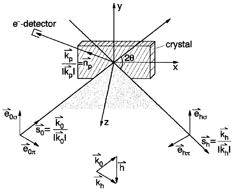
Figure 3: Shematical view of dynamical diffraction and photoelectron yield measurements excited by two coherent electromagnetic waves $\mathbf{E}_{0}(\mathbf{r})$, $\mathbf{E}_{h}(\mathbf{r})$ characterised by the wave vectors $\mathbf{k}_{0}$, $\mathbf{k}_{h}$ and polarization vectors $\mathbf{e}_{0\sigma}$, $\mathbf{e}_{0\pi}$ and $\mathbf{e}_{h\sigma}$, $\mathbf{e}_{h\pi}$. The angle $2\theta$ is the angle between the wave vectors $\mathbf{k}_{0}$ and $\mathbf{k}_{h}$. The direction of the escaping photoelectron is determined by the vector $\mathbf{k}_{\mathbf{p}}$.The relationship of the vectors $\mathbf{k}_{0}$, $\mathbf{k}_{h}$ and $\mathbf{h}$ is indicated.

where $\mathbf{e}_{0}$ and $\mathbf{e}_{h}$ are the unit polarization vectors and $s$ is the polarization index. In the x-ray diffraction theory they are usually defined (see Fig.3) respectively to the so-called scattering plane i.e. the plane containing the vectors $\mathbf{k}_{0}$ and $\mathbf{k}_{h}$. Polarization vectors normal to the scattering plane are called $\sigma-$polarized (in the case of two-wave diffraction $\mathbf{e}_{0\sigma}||\mathbf{e}_{h\sigma}$) and polarization vectors lying in the scattering plane are called $\pi-$polarized (in this case polarization vectors $\mathbf{e}_{0\pi}$ and $\mathbf{e}_{h\pi}$ are misaligned by the angle $2\theta_{B}$).

Now directly from the TT equations (13) for the scalar amplitudes $E_{0}(z)$, $E_{h}(z)$ and for the fixed polarization $s$ we have,

$$\frac{dE_{0s}(z)}{dz} = \frac{i\pi}{\lambda\gamma_{0}}\left[\chi_{00}E_{0s}(z)+\chi_{0h}Ce^{i\varphi(z)-W(z)}E_{hs}(z)\right],$$

$$\frac{dE_{hs}(z)}{dz} = \frac{i\pi}{\lambda\gamma_{h}}\left[\left(\chi_{hh}-\alpha\right)E_{hs}(z)+\chi_{h0}Ce^{-i\varphi(z)-W(z)}E_{0s}(z)\right].$$ (18)

Here $\varphi(z)=\mathbf{hu}(z)$; $\gamma_{0,h}=\cos(\mathbf{n\cdot k}_{0,h})$ are the direction cosines, $\mathbf{n}$ is the inward normal to the entrance surface of the crystal and $\lambda$ is the wavelength of radiation. For Bragg geometry of diffraction $\gamma_{0}>0,\gamma_{h}<0$ and for the Laue diffraction $\gamma_{0}>0,\gamma_{h}>0$. The parameter $\alpha$ is characterizing the deviation of the wave vector k₀ from the exact Bragg condition,

$$\alpha=\frac{k_{h}^{2}-k_{0}^{2}}{k_{0}^{2}}\approx-2\sin 2\theta_{B}\left(\theta-\theta_{B}\right),$$ (19)

where $\theta_{B}$ is the Bragg angle; $C$ is the polarization factor defined as,

$$C=\left\{\begin{array}[]{c}1,\sigma-\mbox{polarization}\\ \cos 2\theta_{B,}\pi-\mbox{polarization}\end{array}\right..$$ (20)

In most of the situations considering only the strongest elastic scattering and the photoelectric scattering process in dipole approximation we have for the Fourier components of the susceptibility in Eq. (18): $\chi_{00}=\chi_{hh}=\chi_{0},\chi_{0h}=\chi_{-h}\equiv\chi\overline{{}_{h}}$ and $\chi_{h0}=\chi_{h}$.

Takagi-Taupin equations (18) have to be supplemented by the boundary conditions, that for a crystal of thickness $L$ have the following form for the different geometries of diffraction

$$\left.E_{0s}(z)\right|_{z=0}=E_{s}^{(in)},\left.E_{hs}(z)\right|_{z=L}=0$$ (21)

for Bragg geometry and

$$\left.E_{0s}(z)\right|_{z=0}=E_{s}^{(in)},\left.E_{hs}(z)\right|_{z=0}=0$$ (22)

for Laue geometry.

Having in mind further applications it is convenient to transform from the set of equations (18) to a single nonlinear equation in the form of the Rikatti equation for the amplitude function

$$R(z,\theta)=\frac{1}{\sqrt{\beta}Y}\left(\frac{E_{hs}(z,\theta)}{E_{0s}(z,\theta)}\right)e^{i\varphi(z)},$$ (23)

where $\beta=\gamma_{0}/|\gamma_{h}|$ for Bragg and $\beta=\gamma_{0}/\gamma_{h}$ for Laue geometries of diffraction and $Y=\sqrt{\chi_{h}/\chi_{\overline{h}}}=\mid Y\mid\exp(i\Phi_{Y})$ (for centrosymmetric crystal with monoatomic lattice $\mid Y\mid=1,\Phi_{Y}=0$). Substituting new function $R(z,\theta)$ (23) into (18) we obtain

$$\mp iL_{ex}\frac{dR(z,\theta)}{dz}=2[-y(\theta)-iy_{0}+y_{\varphi}]R(z,\theta)+C_{1}[1\pm R^{2}(z,\theta)].$$ (24)

Here the upper sign correspond to Bragg diffraction and the lower one for the Laue. We also have introduced the following notations: the angular deviation from the exact Bragg position is measured by the dimensionless parameter,

$$y(\theta)=\sqrt{\beta}\frac{\sin 2\theta_{B}\cdot\left(\theta-\theta_{B}\right)}{X_{r}}\pm\frac{\chi_{0r}(1\pm\beta)}{2\sqrt{\beta}X_{r}},$$ (25)

parameters

$$y_{0}=\pm\frac{\chi_{0i}(1\pm\beta)}{2\sqrt{\beta}X_{r}}\mbox{ and }y_{\varphi}(z)=\pm\frac{L_{ex}}{2}\frac{d\varphi(z)}{dz}$$ (26)

define attenuation of x-rays due to the photoelectric absorption and the shift of the Bragg position due to deformation in a crystal;

$$C_{1}=C\left(1-ip\right)e^{-W(z)},p=-\frac{X_{i}}{X_{r}};$$ (27)

$L_{ex}$ is an extinction length defined as ,

$$L_{ex}=\frac{\lambda\gamma_{0}}{\pi\sqrt{\beta}X_{r}}.$$ (28)

Here we have also introduced the following parameters $X_{r}=Re\sqrt{\chi_{h}\chi_{\overline{h}}}$ and $X_{i}=Im\sqrt{\chi_{h}\chi_{\overline{h}}}$. Now boundary conditions for equation (24) are defined on one surface. For the Bragg case of diffraction we have $R(z)|_{z=L}=0$ and $R(z)|_{z=0}=0$ for Laue case.

The reflectivity is usually defined for Bragg case as

$$P_{R}(\theta)=(1/\beta)\left|E_{h}(0,\theta)/E_{0}(0,\theta)\right|^{2}$$ (29)

now has the following form,

$$P_{R}(\theta)=\left|Y\cdot R(0,\theta)\right|^{2}.$$ (30)

It is easy to obtain solutions of the equation (24) in the case of a perfect thick crystal ($\mu_{0}L>>\gamma_{0}$, where $\mu_{0}$ is a normal absorption coefficient defined as $\mu_{0}=k\chi_{0i}$). In this case $\varphi(z)=0,e^{-W(z)}=1$ and Eq. (24) reduces to an equation with constant coefficients. So, for thick perfect crystal solution does not depend on the thickness of a crystal, that is we have $dR/dz=0$. Now from (24) for Bragg case we obtain directly

$$R_{0}(\theta)=-\frac{1}{C_{1}}\left[\left(-y-iy_{0}\right)+\sqrt{(y+iy_{0})^{2}-C_{1}^{2}}\right],$$ (31)

where for the square root it is chosen the branch with the positive imaginary part.

For the amplitude of the refracted wave $E_{0s}(z,\theta)$ we have directly from the TT equations (18) (and taking into account definition (23))

$$\frac{dE_{0s}(z,\theta)}{dz}=\left[\frac{i\pi\chi_{0}}{\lambda\gamma_{0}}-i\frac{C_{1}}{L_{ex}}R(z,\theta)\right]E_{0s}(z,\theta).$$ (32)

Formal solution of this equation can be written in the following form,

$$E_{0s}(z,\theta)=E_{s}^{(in)}\exp\left[\frac{i\pi\chi_{0}}{\lambda\gamma_{0}}z-i\frac{1}{L_{ex}}\int\limits_{0}^{z}dz^{\prime}C_{1}R(z^{\prime},\theta)\right]$$ (33)

and we have for the intensity of the incident wave,

$$I_{0}(z,\theta)=|E_{0s}(z,\theta)|^{2}=I_{0}^{(in)}\exp\left\{-\frac{\mu_{0}}{\gamma_{0}}z+\frac{2}{L_{ex}}Im\left[\int\limits_{0}^{z}dz^{\prime}C_{1}R(z^{\prime},\theta)\right]\right\}.$$ (34)

In the case of a perfect crystal, $R(z,\theta)\equiv R_{0}(\theta)$ and we have from (34),

$$I_{0}(z,\theta)=I_{0}^{(in)}\exp\left(-\frac{\mu_{in}(\theta)}{\gamma_{0}}z\right)=I_{0}^{(in)}\exp\left\{-\frac{\mu_{0}}{\gamma_{0}}z+\frac{2z}{L_{ex}}Im\left[C_{1}R_{0}(\theta)\right]\right\},$$ (35)

where $\mu_{in}(\theta)$ is an interference absorption coefficient. This expression takes not only into account normal attenuation of x-rays out of the angular region of the dynamical diffraction ($y>>1$)

$$I_{0}(z,\theta)=I_{0}^{(in)}\exp\left\{-\frac{\mu_{0}}{\gamma_{0}}z\right\}$$ (36)

but also takes into account a dynamical ”extinction” effect coming from the multiple scattering of x-rays on atomic planes in the narrow angular region of the dynamical diffraction [1, 2, 3]. In the region of the total reflection for $y\simeq 0$, we obtain from (35)

$$I_{0}(z,\theta)=I_{0}^{(in)}\exp\left\{-\frac{2C}{L_{ex}}z\right\}.$$ (37)

Here we have taken into account also that y${}_{0}<<1$ and $\mu_{0}z<<z/L_{ex}$. From this expression we can see that for the angular position $y=0$ x-rays are effectively attenuated on the typical distances $z\sim L_{ex}$ that for the energies $E\sim 1\div 10keV$ are of the order of microns and are much smaller then normal attenuation distances $z\sim\gamma_{0}/\mu_{0}$ that for the same energies can be of the order of tenth and hundreds of microns (see e.g. [4]).

As we can see from the expression (37) extinction depth $L_{ex}$ is one of the important parameters of the theory that give an effective attenuation distance for x-rays while the dynamical diffraction. In our further treatment all other distances will be compared with $L_{ex}$.

Here we want to make several remarks. The amplitudes $E_{0s}(z,\theta)$ and $E_{hs}(z,\theta)$ in TT equations (18) are complex numbers with its amplitude and phase. Due to the fact that the dynamical scattering is a coherent scattering process this two amplitudes are connected with each other and, for example, in the case of a perfect crystal on its surface we have from (23) for the ratio of these amplitudes on the surface of the crystal

$$\left.\frac{E_{hs}(z,\theta)}{E_{0s}(z,\theta)}\right|_{z=0}=\frac{|E_{h}(\theta)|}{|E_{0}(\theta)|}e^{i\alpha(\theta)}=\sqrt{\beta}YR_{0}(\theta),$$ (38)

where $R_{0}$ is defined in (31).

Typical behavior of the reflectivity $P_{R}(\theta)$ and of the phase $\alpha(\theta)$ in the diffraction region is shown on Fig. 4. In this small angular region typically of several arcsec the reflectivity $P_{R}(\theta)$ is of the order of unity and the phase $\alpha(\theta)$ of the wave field changes from $-\pi$ to $0$ . Just this fast change of the phase makes x-ray standing wave method so sensitive to any additional phase shifts.

2.2 Susceptibilities

The Fourier components of the susceptibility $\chi_{0}$ and $\chi_{h}$ (see expansion (7)) are in general complex valued [3]

$$\chi_{h}=\chi_{hr}+i\chi_{hi}.$$ (39)

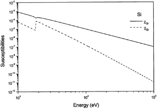
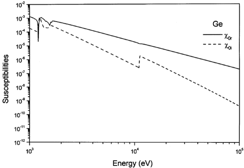
Figure 5: The values of the zero Fourier components of the susceptibilities $\chi_{0r}$ and $\chi_{0i}$ calculated for $Si$ and $Ge$ as a functions of energy $E$ [41].

The real part $\chi_{hr}$ correspond to elastic scattering of x-rays and imaginary part $\chi_{hi}$ accounts for absorption effects. The values of $\chi_{hr}$ and $\chi_{hi}$ are calculated from quantum mechanics (see Fig.5, where the values of $\chi_{0r}$ and $\chi_{0i}$ are calculated for $Si$ and $Ge$ for different energies) and for crystals without center of symmetry may themselves be complex [3]. For hard x-ray energy range $(E\sim 1\div 10keV)$ $\chi_{hr}$ is negative and for the most of elements is of the order of $10^{-6}$. It is convenient to present it in the following form [3],

$$\chi_{hr}=-\left(\frac{r_{0}\lambda^{2}}{\pi\Omega}\right)F_{hr},F_{hr}=\sum\limits_{j}\left(f_{j}+\Delta f_{j}\right)e^{-W_{j}^{T}}e^{-i\mathbf{h\rho}_{j}}.$$ (40)

Here $r_{0}=e^{2}/mc^{2}=2.818\cdot 10^{-15}m$ is the classical electron radius, $\Omega$ is the unit cell volume and $F_{hr}$ is the structure factor for the reciprocal lattice vector $\mathbf{h}$. Expression (40) is written for an arbitrary unit cell of a crystal, summation is made over all atoms of the unit cell, $\mathbf{\rho}_{j}$ is the coordinate of the $j-$th atom in a unit cell; $e^{-W_{j}^{T}}$ is the thermal Debye-Waller factor that takes into account the attenuation of the elastic scattering of x-rays due to a thermal vibrations of the atoms. In equation (40)

$$f_{j}(\mathbf{h})=\int n(\mathbf{r})e^{i\mathbf{hr}}d\mathbf{r}$$ (41)

is an atomic scattering factor for the $j-$th atom in a unit cell. It is determined by the electron density $n(\mathbf{r})$ in an atom and $\Delta f_{j}$ is an account for the dispersion corrections to an atomic scattering factor. The values of this parameters are tabulated in International Tables for X-ray Crystallography [4].

As it was already mentioned above, the imaginary part of the susceptibility $\chi_{hi}$ takes into account absorption effects. For hard x-rays $(E\sim 1\div 10keV)$ its value (see Fig.5) is two orders of magnitude smaller then the real part $\chi_{hr}$ $(\chi_{hi}\sim 10^{-7}\div 10^{-8})$ and, for our choice of the phase in the plane wave (11), it is positive. It can be shown [33, 42] that in general case the imaginary part of susceptibility $\chi_{hi}$ contains contributions from all the inelastic processes: the photoelectric absorption, Compton scattering and thermal diffuse scattering

$$\chi_{hi}=\chi_{hi}(Ph)+\chi_{hi}(CS)+\chi_{hi}(TDS).$$ (42)

The imaginary part of the Fourier component of the susceptibility $\chi_{hi}$ in a crystal in analogy to (40) can also be presented as a sum of contributions of different atoms

$$\chi_{hi}=\left(\frac{\lambda}{2\pi\Omega}\right)\sum\limits_{j}\sigma_{j}e^{-W_{j}^{T}}e^{-i\mathbf{h\rho}_{j}},$$ (43)

where $\sigma_{j}$ are the cross sections of the different inelastic processes for the $j-$th atom in the unit cell and their values can be obtained from [4, 43].

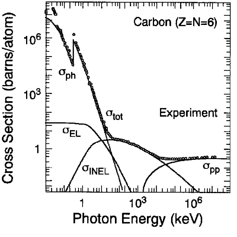
Figure 6: Calculated cross-sections for photon scattering from carbon showing the contributions of photoelectric, elastic (Rayleigh), inelastic (Compton), and pair-production cross-sections. Also shown are the experimental data (open circles). From Ref. [4]. Even for the light element carbon, the photoelectric cross-section is clearly dominating in the x-ray energy range up to more than 100 keV.

As it was pointed out previously in general case the susceptibility of a crystal is a tensor and has a non-local character. Being interested in diffraction and taking into account relationships between the values of the cross sections of the different processes (see Fig.6)

$$\sigma_{T}>>\sigma_{Ph}>>\sigma_{C}\geq\sigma_{TDS},$$ (44)

where $\sigma_{T},\sigma_{Ph},\sigma_{C},\sigma_{TDS}$ are the cross sections of the elastic Thompson scattering, photoelectric absorption, Compton scattering and thermal diffuse scattering we can neglect in (18) small non-local corrections to $\chi_{h}$ and treat susceptibilities as scalar values. However analysing the yield of the secondary radiation while the dynamical diffraction of x-rays this corrections may be essential and can not be neglected. For example, while considering Compton and thermal diffuse scattering it is necessary to account tensor character of $\chi_{hi}$ and the angular dependence of the corresponding cross sections of the inelastic scattering (see for e.g. [44, 45, 46]). Different situation is realized for practically valuable case of fluorescence radiation and photoelectron emission (according to (44) it is the main inelastic process). So far as these processes are caused by photoelectron absorption, the total value of each in dipole approximation does not depend from the direction of propagation of the radiation in an isotropic crystal the imaginary part of the susceptibilities can be treated as scalar values and without angular dependence. Further, if not mentioned specially, we shall consider mainly this case.

Takagi-Taupin equations (18) were obtained in the dipole approximation. Small quadrupole corrections in imaginary part of $\chi_{hi}$, if necessary, can be also taken into account. They will bring to renormalization of the polarization factor $C$, that can become essential for scattering near adsorption edges and backscattering (see for details [47, 48, 49]).

3 Theory of x-ray standing waves in a real crystal (general approach)

In this Chapter we shall obtain, using the approach of Afanasev and Kohn [32], the general expression for the yield of the secondary radiation in the case of the dynamical diffraction of X-rays from the deformed crystal lattice. The amplitudes of the waves $E_{0}(z,\theta)$ and $E_{h}(z,\theta)$ in such a crystal can be obtained from the TT equations (18) (we shall consider deformations that depend only from $z$).

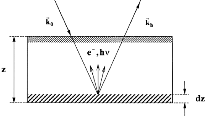
Figure 7: Part of x-ray radiation while scattering on crystal is absorbed in a layer with the thickness $dz$ at the depth $z$ and gives rise to the yield of the secondary radiation (photoelectron $e^{-}$, fluorescence $h\nu$, etc.).

To find the intensity of the secondary radiation yield at the depth $z$ in a crystal, one must determine the number of absorbed quanta in a layer with the thickness $dz$ per unit area and unit time (Fig. 7). It is proportional to the loss of the energy field in this layer. From the equation of the field energy balance we have for the number of absorbed quanta

$$\hbar\omega\frac{dN(z)}{dz}=-div\mathbf{S}(z)=-\frac{dS_{z}}{dz},$$ (45)

where $\mathbf{S}(z)$ is the energy flow (Poynting vector), averaged over the time period of the field oscillations and over the elementary cell of the crystal. In (45) we have taken into account that $\mathbf{S}(z)$ depend only from $z$.

According to the definition of the energy flow vector

$$\mathbf{S}(z)=\frac{c}{8\pi}\left[\mathbf{s}_{0}|E_{0}(z)|^{2}+\mathbf{s}_{h}|E_{h}(z)|^{2}\right],$$ (46)

where $\mathbf{s}_{0}=\mathbf{k}_{0}/|k_{0}|$ and $\mathbf{s}_{h}=\mathbf{k}_{h}/|k_{h}|$ are the unit x-ray propagation vectors, we can obtain for the number of absorbed quanta,

$$\frac{dN(z,\theta)}{dz}=-\frac{c}{8\pi\hbar\omega}\left[\gamma_{0}\frac{d|E_{0}(z,\theta)|^{2}}{dz}+\gamma_{h}\frac{d|E_{h}(z,\theta)|^{2}}{dz}\right].$$ (47)

Taking into account TT equations (18) we have

$$\frac{dN_{m}(z,\theta)}{dz} = \frac{ck}{8\pi\hbar\omega}\{E_{0}^{*}(z,\theta)\chi_{00,i}(m)E_{0}(z,\theta)+$$

$$\ E_{h}^{*}(z,\theta)\chi_{hh,i}(m)E_{h}(z,\theta)+$$

$$\ 2Re[E_{0}^{*}(z,\theta)\chi_{0h,i}(m)E_{h}(z,\theta)\exp(i\varphi(z)-W(z))]\}.$$

The number of absorbed quanta is determined only by the imaginary part of the susceptibility $\chi_{hi}$ that is account for absorption effects. According to (42) it is possible to separate the influence of the different processes into the yield of the secondary radiation. The index $m$ introduced in (3), characterizes this contribution of a certain secondary process, which is under investigation.

The total number of the secondary quanta emitted from the crystal is equal to

$$N_{m}(\theta)=\int\limits_{0}^{\infty}dzP_{yi}^{m}(z)\frac{dN_{m}(z,\theta)}{dz},$$ (49)

where $P_{yi}^{m}(z)$ is the probability function of the yield of the secondary radiation of the type $m$ from the depth $z$.

Equations (3-49) are general and give the solution for the problem of the angular dependence of the secondary radiation yield, when x-ray standing wave exist in a crystal. They are valid for any type of inelastic process such as photoeffect, fluorescence radiation, Compton scattering and thermal diffuse scattering. They can be applied as well for investigation of secondary electrons, i.e. Auger electrons and electrons ejected due to absorption of fluorescence radiation. One must only define the values of the Fourier components of the susceptibility $\chi_{00,i},\chi_{hh,i}$, and $\chi_{0h,i}$ appropriately, as well as the probability function $P_{yi}^{m}(z)$. The amplitudes $E_{0}(z,\theta)$ and $E_{h}(z,\theta)$, naturally, does not depend on the type of the inelastic process that is experimentally registered, but are determined only by the diffraction process on a real crystal. If, for example, the deformation field $\mathbf{u}(z)$ and the level of amorphization $W(z)$ are known, then the amplitudes $E_{0}(z,\theta)$ and $E_{h}(z,\theta)$ can be obtained directly from the TT equations (18). On Fig. 8 results of calculations of the reflectivity curves and photoeffect yield for the silicon crystal with the known profile of deformation (also shown on Fig. 8) are presented. The series of curves correspond to both the entire layer (upper curves) and to parts of it.

In most of the applications of XSW method it is assumed, that the yield of the inelastic process under investigation is completely determined by the intensity of the wavefield at the atoms positions. However, according to result summarized in Eqs. (3–49), it is not always fulfilled. In fact there are two main effects that are taken into account. This is first of all the deformation of a crystal lattice described by an additional phase factor $\varphi(z)$ (due to the displacement of atomic planes) and the static Debye-Waller factor $e^{-W(z)}$ (due to the random displacements of atoms) in the third term of (3). The second effect is coming from non-locality of some of the inelastic processes. This can be, for example, effects of higher order multipole interactions for the photoeffect processes [48, 49] or non-local character of such processes as Compton scattering or thermal diffuse scattering [44, 45, 46].

Being interested in future mainly by the fluorescence and photoelectron yield in dipole approximation we can write Eq. (3) in the following form (further we will omit index $m$ and assume, that $\chi_{00,i}=\chi_{hh,i}\equiv\chi_{0i}$ and $\chi_{0h,i}\equiv\chi_{\overline{h}i}$),

$$\frac{dN(z,\theta)}{dz} = \frac{c\mu_{0}}{8\pi\hbar\omega}|E_{0}(z,\theta)|^{2}\{1+\frac{|E_{h}(z,\theta)|^{2}}{|E_{h}(z,\theta)|^{2}}+$$ (50)

$$\ \ +2Re[\varepsilon_{\overline{h}}\frac{E_{h}(z,\theta)}{E_{0}(z,\theta)}e^{i\varphi(z)-W(z)}]\},$$

where

$$\varepsilon_{\overline{h}}=\frac{\chi_{\overline{h}i}}{\chi_{0i}}=\frac{\sum\limits_{j}\sigma_{j}e^{-W_{j}^{T}}e^{-i\mathbf{h\rho}_{j}}}{\sum\limits_{j}\sigma_{j}}.$$ (51)

Now substituting into (50) the expression for the amplitude $R(z,\theta)$(23) we have for the normalized intensity yield of the secondary process

$$\kappa(\theta) = \frac{I(\theta)}{I(\infty)}=\frac{1}{I(\infty)}\int\limits_{0}^{\infty}dzP_{yi}(z)|E_{0}(z,\theta)|^{2}\{1+\beta|Y|^{2}|R(z,\theta)|^{2}+$$ (52)

$$+2\sqrt{\beta}e^{-W(z)}CRe[\varepsilon_{\overline{h}}YR(z,\theta)]\},$$

where intensities are usually normalized by their values far from the region of the Bragg diffraction $I(\infty)=\int\limits_{0}^{\infty}dzP_{yi}^{m}(z)|E_{0}(z,\infty)|^{2}$.

Equation (52) together with equations (24, 30) and (35) completely determine the scheme of calculation of the angular dependence of the yield of the secondary radiation in the most general case under the condition that a plane wave is incident on the crystal. In a real experimental situation the experiment is performed in a double-crystal scheme with a first crystal-monochromator. In this case for the comparison of theoretical calculations with the experimental results the convolution between the curve of the secondary radiation yield and the reflectivity curve of the monochromator crystal has to be calculated. If an asymmetric reflection is used in both crystals, i.e. asymmetry factor $\beta$ in the sample crystal and the asymmetry factor of the monochromator crystal $\beta_{1}$ do not equal to unity, then we have for the convoluted curve of the SR yield

$$\overline{\kappa}(\theta)=\frac{I(\theta)}{I(\infty)}=\frac{\sum\limits_{s}\int\limits_{-\infty}^{+\infty}dy_{1}P_{R}^{(s)}\left(y_{1}\right)\kappa^{(s)}\left(y(\theta)+\sqrt{\beta\beta_{1}}y_{1}\right)}{\sum\limits_{s}\int\limits_{-\infty}^{+\infty}dy_{1}P_{R}^{(s)}\left(y_{1}\right)}.$$ (53)

Here $\theta$ is the angle between the reflecting planes of the crystal-monochromator and the sample crystal and summation in Eq. (53) is performed over the different polarization states. Convolution with the reflectivity curve (30) of the sample $\overline{P_{R}}(\Delta\theta)$ is defined in the same way.

Finally, in this Section we have formulated the main equations for the SR yield excited by XSW while the dynamical diffraction of x-rays in real crystals. In the remainder of the work we will analyse different physical applications to this general formalism.

4 XSW in a perfect crystal

In this Chapter we shall consider an effects of registration of the different inelastic processes in a simple case of a perfect crystal. Though it is the most simple case of the real crystal, the main peculiarities of the XSW field and SR yield can be already revealed and understood in this case. In the end of the Chapter the case of amorphous layer on the top of the perfect one is shortly discussed as well.

4.1 XSW with a big and small depth of yield (extinction effect)

In the case of the perfect crystal the amplitude $R(z,\theta)\equiv R_{0}(\theta)$ (see Eq. (31)) and it does not depend from the coordinate $z$. From (52) we obtain for the wave field intensity,

$$I(\theta)=\{1+\beta|Y|^{2}|R_{0}(\theta)|^{2}+2\sqrt{\beta}CRe[\varepsilon_{\overline{h}}YR_{0}(\theta)]\}\int\limits_{0}^{\infty}dzP_{yi}(z)|E_{0}(z,\theta)|^{2}.$$ (54)

In the limit when we can neglect the angular dependence in the last integral and in addition if approximation $\varepsilon_{\overline{h}}=\chi_{\overline{h}i}/\chi_{0i}=1$ is valid we are coming to the well known expression for the wave field intensity (2). From the above expression we can see that the shape of the curve of the SR from the perfect crystal is mainly determined by two factors. First of all it depend on the depth of yield $L_{yi}$ of the SR that is determined by the probability yield function $P_{yi}(z)$ and, secondly, in the case of detecting SR process from the multicomponent crystal its shape essentially depend from the complex factor $\varepsilon_{\overline{h}}$. In the beginning we shall consider effects of the depth of yield.

For the future analysis it is convenient to take the probability yield function $P_{yi}(z)$ in the form of an exponential function:

$$P_{yi}(z)=\exp(-\mu_{yi}^{eff}z).$$ (55)

This form of the probability function is exact for the yield of the fluorescence radiation with $\mu_{yi}^{eff}=\mu_{yi}^{fl}/\gamma_{fl}$, where $\mu_{yi}^{fl}$ is an attenuation coefficient of the specific fluorescence line, that is measured in experiment and $\gamma_{fl}$ is the cosine of the exit angle of this fluorescence radiation. For the case of photoeffect integrated over all the directions of the photoelectron yield this form of $P_{yi}(z)$ with $\mu_{yi}^{eff}=2.3/L_{yi}^{ph}$, where $L_{yi}^{ph}$ is an average escape depth of electrons is a good approximation [51] to probability yield function obtained from the Monte-Carlo simulations [52, 53]. For the escape depth of the electrons with an initial energy $E_{i}$ (in $keV$) the following approximation formula can be used

$$L_{yi}^{ph}(E_{i})=780E_{i}^{2}/\rho\ln(E_{i}/E_{0}),$$ (56)

where $\rho$ is the density of the material in $g\cdot cm^{-3}$and $E_{0}\approx 0.39keV$.

Taking now into account that according to Eq. (35) for the perfect crystal $|E_{0}(z,\theta)|^{2}=|E_{0}^{(in)}|^{2}\exp(-\mu_{in}(\theta)z/\gamma_{0})$, we obtain from (54) for the yield of the secondary radiation from a perfect crystal

$$I(\theta)=\frac{I^{SW}(\theta)}{\mu_{yi}^{eff}+\mu_{in}(\theta)/\gamma_{0}},$$ (57)

where

$$I^{SW}(\theta)=1+\beta|Y|^{2}|R_{0}(\theta)|^{2}+2\sqrt{\beta}CRe[\varepsilon_{\overline{h}}YR_{0}(\theta)].$$ (58)

Now we can easily analyse different limits of the depth of yield parameter on the angular dependence of the SR curve. For example, in the limit when the escape depth of the secondary radiation $L_{yi}$ is much smaller then the minimum penetration depth $L_{ex}$ of the standing wave field into a crystal ($L_{yi}<<L_{ex}$) $\mu_{yi}^{eff}>>\mu_{in}(\theta)$ and from Eq. (57), we obtain

$$I(\theta)=\frac{I^{SW}(\theta)}{\mu_{yi}^{eff}}\left[1-\frac{1}{\gamma_{0}}\frac{\mu_{in}(\theta)}{\mu_{yi}^{eff}}\ldots\right].$$ (59)

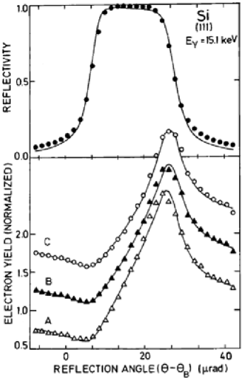
Figure 9: Left: Angular dependence of the yield of $GeK_{\alpha}$ fluorescence and of x-ray reflection in (111) diffraction of $MoK_{\alpha}$ radiation. The fluorescence data are measured with a $Si(Li)$ detector situated at a glancing angle to the surface, the value of which is indicated in milliradians. From Ref. [54]; Right: The angular variation of the perfect $Si$ (111) reflectivity and photoelectron yields while diffraction of x-ray radiation with energy $E=15.1$ $keV$. Photoelectron curves correspond to electrons with different energy losses $\Delta E$ ($\Delta E=0$ (A)$,2.5$ (B) and $5$ $keV$ (C) respectively). From Ref. [55].

The angular dependence of the SR yield in this limit is mainly determined by the intensity variation of the standing wave field through the atomic planes (Eq.(58)). Its shape for the monoatomic crystal will totally coincide with the intensity variation of the wave field (2). At the same time, following Eq. (59) the maximum change in the shape of the intensity curve is due to an extinction effect that can be seen only in the central region of the total reflection. It leads to a weak variation in the slope of the linear part, i.e., to a weak decline in the intensity yield at this angles. It is interesting to note here, that this actual form of the standing wave curve contain information about the real escape depth of the secondary radiation, that can be obtained by fitting experimental data to theoretical calculations in the form of equation (59). This effects were observed experimentally in the case of the fluorescence radiation [54] (change of the depth of yield $L_{yi}$ was obtained by the change of the exit angle of the fluorescence yield) and in the case of photoeffect [55] (see Fig. 9).

Now we shall consider opposite limit of the big depth of yield ($L_{yi}>>L_{ex}$). This is the typical situation in the case of measuring fluorescence radiation from the atoms of a crystal lattice or for the measuring of the inelastic scattering on thermal phonons. For the analysis of this limit it is useful to use in Eq. (54) the following expression (see for e.g.[2]),

$$\mu_{0}\left\{1+\beta P_{R}(\theta)+2\sqrt{\beta}Re\left[\varepsilon_{\overline{h}}R_{0}(\theta)\right]\right\}=\mu_{in}(\theta)\left[1-P_{R}(\theta)\right]$$ (60)

and now we obtain for the yield of the SR,

$$I(\theta)=\left[1-P_{R}(\theta)\right]\frac{\mu_{in}(\theta)/\mu_{0}}{\mu_{yi}^{eff}+\mu_{in}(\theta)/\gamma_{0}}\simeq\left[1-P_{R}(\theta)\right]\left[1-\gamma_{0}\frac{\mu_{yi}^{eff}}{\mu_{in}(\theta)}\right].$$ (61)

In the case of the fluorescence radiation we have for the intensity

$$I^{fl}(\theta)=\left[1-P_{R}(\theta)\right]\left[1-(\gamma_{0}/\gamma_{fl})(\mu_{yi}^{fl}/\mu_{in}(\theta))\right].$$

As we can see from Eq. (61) now in the limit of the big depths of yield $\mu_{yi}<<\mu_{in}(\theta)$ the shape of the SR curve has the form of the reverse curve of the reflectivity $I(\theta)\simeq\left[1-P_{R}(\theta)\right]$. This result has a simple physical explanation. Really, in the angular region of the dynamical scattering x-rays does not penetrate deeper than the extinction depth $L_{ex}$, so, SR can be excited only from this depths. Due to the law of the energy conservation the yield of the SR has to be equal to Eq. (61). However, if the term $\gamma_{0}\mu_{yi}^{eff}/\mu_{in}(\theta)$ in expansion (61) is becoming comparable with unity, then on the curves of the secondary radiation one can see small asymmetry due to the behavior of $\mu_{in}(\theta)$. This behavior of the fluorescence radiation was for the first time measured and understood in the pioneer works of B. Batterman [6, 7] and then repeated in many other works (see for e.g. Fig. 10).

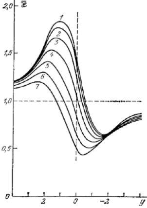
Figure 11: Angular dependences of the secondary radiation yield calculated for $Si$ (400) reflection and $CuK_{\alpha}$ radiation for different values of the ratio $L_{ex}/L_{yi}$ equal to: 12 (1), 7.2 (2), 3.6 (3), 1.8 (4), 0.9 (5), 0.45 (6), and 0.225 (7), in a system with a symmetric monochromator. From Ref. [11].

It is clear, that using the depth of yield $L_{yi}$ as a parameter we will obtain a number of curves that lie between two limiting cases described by Eq. (59) and (61). On Fig. 11 the calculated curves of the angular dependence of the SR yield from a perfect $Si$ crystal are presented. For calculations it was used the case of (400) diffraction of $CuK_{\alpha}$ radiation ($L_{ex}=3.60\mu m$) for different values of the parameter $L_{yi}$.

4.2 Multicomponent crystals

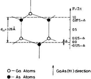
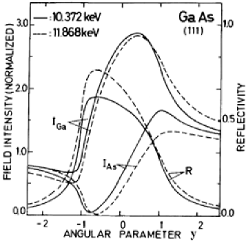
Figure 12: Top: Schematic view showing the position of the noncentrosymmetric $GaAs(111)$ diffraction planes (dashed lines) relative to the $Ga$ atoms (open circles) and $As$ atoms (closed circles). Parameter $P_{c}$ locates positions in this structure in the (111) direction relative to a (111) diffraction plane, which is shifted by an amount $\Delta$ relative to a centrosymmetric (111) diffraction plane; Bottom: Angular dependence of the wave field intensity in a $GaAs(111)$ crystal at the $Ga$ ($I_{Ga}$) and $As$ ($I_{As}$) atomic sites for x-ray diffraction with an energy of $10.372$ $keV$ (solid line) and $11.868$ $keV$ (dotted line) for $\sigma-$polarization. The energies of radiation are chosen to be $5$ $eV$ above the $GaK$ and $AsK$ edges. From Ref. [57].

In a perfect crystals with the complicated elementary cell containing different type of atoms XSW method give a unique possibility to investigate position and degree of disorder of different type of atoms. Experimentally the most effective way to do it is to register the characteristic fluorescence radiation from different atoms. The nodes and antinodes of x-ray standing wave are located in the different way for different sublattices of the crystal (on Fig. 12a (111) diffraction planes of $GaAs$ crystal are shown). In this situation the angular dependence of the fluorescence yield for different type of atoms will have the different shape and also will differ from the typical curves of the monoatomic crystals (see for e.g. Fig.12b for the same case of $GaAs$ crystal).

Peculiarities of the angular dependence of the fluorescence yield in a multicomponent perfect crystal are determined in fact solely by the factor $\varepsilon_{\overline{h}}$ in (54). If we are interested by the yield of the fluorescence radiation from the atom of the sort $a$ from a multicomponent crystal then we have for the factor $\varepsilon_{\overline{h}}$ in (54) (see also (43)),

$$\varepsilon_{\overline{h}}^{a}=\frac{\chi_{\overline{h}i}}{\chi_{0i}}=\left(\frac{\sigma_{a}(\mathbf{h})}{\sigma_{a}(0)}\right)\frac{\sum\limits_{j}c_{j}^{a}e^{-W_{j}^{a}(h)}S_{j}^{a}(\overline{\mathbf{h}})}{\sum\limits_{j}c_{j}^{a}},$$ (62)

where $c_{j}^{a}$ is the concentration of the atoms of the sort $a$ in the sublattice $j$, $\sigma_{a}(0)$and $\sigma_{a}(\mathbf{h})$are the cross sections of the corresponding processes, $e^{-W_{j}^{a}(h)}$ are the Debye-Waller factors (here they are the sum of thermal and static displacements) and $S_{j}^{a}(\overline{\mathbf{h}})=\sum\limits_{j^{\prime}}e^{i\mathbf{h\rho}_{j^{\prime}}^{a}}$are the structure factors corresponding to the positions of the atoms of the sort $a$ in the unit cell. The total cross sections of the photoexcitation in dipole approximation are isotropic and we have for $\sigma_{a}(\mathbf{h})/\sigma_{a}(0)=1$, however if quadrupole contributions are valuable we have for the ratio of cross sections in Eq. (62)

$$\frac{\sigma_{a}(\mathbf{h})}{\sigma_{a}(0)}=1-\frac{\sigma_{a}^{Q}}{\sigma_{a}}\left(1-\frac{C^{Q}}{C}\right),$$ (63)

where $\sigma_{a}=\sigma_{a}^{D}+\sigma_{a}^{Q},\sigma_{a}^{D}$ and $\sigma_{a}^{Q}$ are the total, dipole and quadrupole cross sections correspondingly, $C$ is the polarization coefficient (20) and parameter $C^{Q}$ is equal to $\cos 2\theta_{B}$ for $\sigma-$ polarization and $\cos 4\theta_{B}$ for $\pi-$ polarization (see for details [48, 49]). This can be important while measuring fluorescence radiation near absorption edges or in a backscattering geometry, where quadrupole contribution can be essential. Expression (62) is simplified for the case of two-component crystals when different type of atoms occupy different sublattices (this is the case of $GaAs$, $InSb$ and etc. crystals). In this case we have from Eq. (62)

$$\varepsilon_{\overline{h}}^{a}\simeq e^{-W^{a}(h)}S^{a}(\overline{\mathbf{h}})=e^{-W^{a}(h)}\mid S^{a}(\overline{\mathbf{h}})\mid e^{i\varphi^{a}(\mathbf{h})},$$ (64)

where dipole approximation is assumed. Structure factors $S_{j}^{a}(\overline{\mathbf{h}})$ are complex quantities with their amplitude $\mid S^{a}(\overline{\mathbf{h}})\mid$ and phase $\varphi^{a}(\mathbf{h})$. Substituting this values of $\varepsilon_{\overline{h}}(a)$ into expression (58) we obtain for the intensity of standing wave on the positions of the atoms of the sort $a$,

$$I^{SW}(\theta)=1+\beta|Y|^{2}|R_{0}(\theta)|^{2}+2\sqrt{\beta}C\mid YR_{0}(\theta)\mid F_{c}^{a}(h)\cos\left[\alpha(\theta)+\varphi^{a}(\mathbf{h})+\Phi_{Y}\right],$$ (65)

where

$$F_{c}^{a}(h)=e^{-W^{a}(h)}\mid S^{a}(\overline{\mathbf{h}})\mid.$$ (66)

This is an important result. According to Eq.(65) the angular dependence of the SR yield directly depend on the phase $\varphi^{a}(\mathbf{h})$ of the structure factor $S_{j}^{a}(\overline{\mathbf{h}})$. Moreover, due to the fact that this phase enter the interference term in (65) the angular dependence of the field intensity $I^{SW}(\theta)$ is very sensitive to the value of this phase. So, measuring this angular dependence one can determine with high accuracy the phase and the amplitude $\mid S^{a}(\overline{\mathbf{h}})\mid$ of the structure factor for different sublattices (or different sort of atoms) in multicomponent crystals. In this way the $\mathbf{h}-$th Fourier component of the structure factor can be totally determined [58]. This is illustrated for the case of the $GaAs$ crystal on Fig.12. Of course according to our previous discussion this initial curve will be modified when the final depth of yield of the fluorescence radiation (Eq. (57)) will be taken into account.

This idea of measuring the SR (fluorescence or photoelectron yield) in the XSW field in multicomponent perfect crystals was successfully realized in a number of experiments. For example, the polarity of $GaP$ crystals was obtained in experiments [59] while monitoring fluorescence radiation and in experiments [60] $GaL$ photoelectrons were measured using a cylindrical energy analyzer in a high-vacuum chamber. Due to a high sensitivity of XSW method it has become possible to measure the change of the phase of the structure factor as a function of energy near absorption edges in noncentrosymmetric crystals (see for e.g. [57, 61] and also theoretical paper [62]). In the paper [63] it was demonstrated the possibility of determination of the positions of the Ga and Gd atoms in the unit cell (it contain 160 atoms) of the perfect garnet crystals while monitoring characteristic fluorescence radiation in the XSW field. In a recent papers the fluorescence radiation from different atoms in the unit cell of High-T_c crystal was measured [64], positions of $Cd,Zn,Se$ and $Te$ atoms in $Cd_{1-x}Zn_{x}Se_{y}Te_{1-y}$ single crystals were obtained [65].

Analysis of the photoelectron yield (especially if Auger electrons are monitored) while scanning XSW in multicomponent crystals is more complicated comparing to the fluorescence yield. Really, even if detectors with high energy resolution are available then the contribution to the total photoelectron yield in the registered energy range is in general the sum of contributions of primary photoelectrons ejected from different atomic subshells and from different sort of atoms. Finally we have [12]

$$Y_{el}(E,\theta)=\sum\limits_{N,a}g_{Na}Y_{Na}(E,\theta),$$ (67)

where for the case of perfect crystals $Y_{Na}(E,\theta)$ is determined by Eq. (54) with the factor $\varepsilon_{\overline{h}}=\varepsilon_{\overline{h}}^{a}(N)$ equal to that of (62) and with $P_{yi}(z)=P_{Na}(z,E)$, that determines now the probability of the photoelectron escape with energy $E$ ejected at the depth $z$ from the $N-$th subshell of the $a-$th sort of atom. Parameter $g_{Na}$ determines the fraction of electrons ejected from the $N-$th subshell of the $a-$th sort of atom to the total number of such electrons,

$$g_{Na}=\frac{n_{a}\sigma_{Na}(0)}{\sum\limits_{N,a}n_{a}\sigma_{Na}(0)},$$ (68)

where $n_{a}$ is a number of atoms of the $a-$th sort in a unit cell. Taking into account, that typically the photoelectron yield depth of yield is much smaller, then the extinction depth ($L_{yi}<<L_{ex}$) we can use for the photoelecton yield expression (58) with the parameter $\varepsilon_{\overline{h}}$ equal to,

$$\varepsilon_{\overline{h}}=\sum\limits_{N,a}g_{Na}\varepsilon_{\overline{h}}^{a}(N)P_{Na}(E),$$ (69)

where $P_{Na}(E)=\int\limits_{0}^{\infty}P_{Na}(z,E)dz$.

4.3 Crystals with an amorphous surface layer

We shall assume now, that the top of the crystal contain thin amorphous layer with the thickness $L_{am}$. We shall also assume, that the depth of yield of the SR is much smaller, then the extinction depth, but bigger then the thickness of amorphous layer $L_{am}<L_{yi}<<L_{ex}$ (this can be the photoelectron yield for example). It is clear, that in amorphous layer there is no interference between incident and diffracted beam and we can neglect small attenuation of x-rays in this thin layer. Taking all this into account and performing integration in (52) separately in amorphous and in the perfect part of a crystal we obtain,

$$\kappa(\theta)=p_{am}\kappa^{am}(\theta)+(1-p_{am})\kappa^{id}(\theta),$$ (70)

where

$$\kappa^{am}(\theta)=1+\beta P_{R}(\theta),$$ (71)

$$\kappa^{id}(\theta)=I^{SW}(\theta)=1+\beta P_{R}(\theta)+2\sqrt{\beta}CRe[\varepsilon_{\overline{h}}YR_{0}(\theta)]$$ (72)

and $p_{am}$ is amorphous fraction of the crystal defined as

$$p_{am}=\int\limits_{0}^{L_{am}}P_{yi}(z)dz.$$ (73)

In (70-73) we are assuming, that the depth of yield function is normalized to unity $\int\limits_{0}^{\infty}P_{yi}(z)dz=1.$

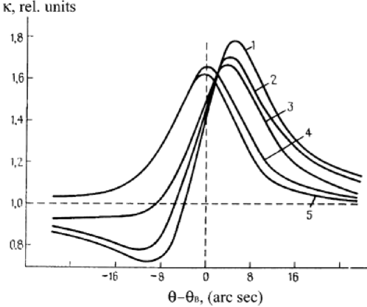
Figure 13: Angular dependences of the photoelectron yield for $Ge(220)$ diffraction, $CuK_{\alpha}$ radiation with different thickness of amorphous layers on the surface: 0 (1), 50 (2), 100 (3) 250 (4) 450 (5) $nm$. From Ref. [66].

From expressions (70-72) we see, that in general for different thickness of amorphous layers we obtain different shape of the curves of the photoelectron yield all lying between two curves $\kappa^{id}(\theta)$ for perfect crystal and $\kappa^{am}(\theta)$ for amorphous layer $L_{am}>L_{yi}$. Such measurements were made in [66, 67] and are presented on Fig.13.

In general escape depth of electrons $L_{yi}(E_{i})$ from the crystal depend from the initial energy $E_{i}$ (see for e.g. Eq. (56)). Assuming now exponential probability yield function in the form (55)

$$P_{yi}(E_{i})=\frac{1}{L_{yi}(E_{i})}\exp(-\frac{z}{L_{yi}(E_{i})})$$

we obtain for the amorphous fraction of the crystal $p_{am}$

$$p_{am}=1-\exp[-L_{am}/L_{yi}(E_{i})].$$ (74)

From this expression we have for the ratio $L_{am}/L_{yi}(E_{i})$

$$L_{am}/L_{yi}(E_{i})=-\ln(1-p_{am}).$$ (75)

Now, if one of the parameters: thickness of amorphous layer $L_{am},$ or escape depth of electrons $L_{yi}(E_{i})$ is known, then another one can be obtained from Eq. (75).

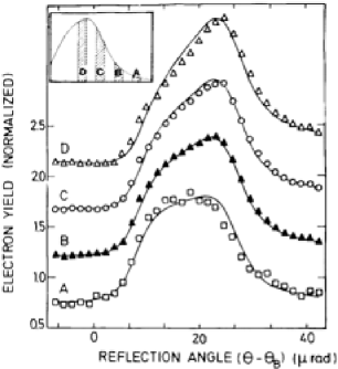
Figure 14: The angular variation of the 0.6-$\mu m$ $SiO_{2}/Si(111)$ photoelectron yields for energy regions A-D of the emission spectrum (shown in the inset). The solid lines are theoretical curves. From Ref. [55].

This idea was realized in the paper [55] (see Fig. 14), when the photoelectron yield for different group of electrons with different loss of energy was measured with the low-resolution gas-proportional counter. In this experiments escape depth $L_{yi}=1.2$ $\mu m$ for the initial energy of the electrons $E_{i}=13.3$ $keV$ in Si crystal with amorphous SiO₂ layer was obtained.

5 Bicrystal model (Bragg geometry)

5.1 Theory

The calculation scheme of the angular dependence of the SR yield $\kappa(\theta)$ for the Bragg geometry of x-ray diffraction in the crystals with the deformed surface layer was developed in [50]. In general case when the deformation profile of the crystal lattice has an arbitrary profile the main problem is to solve nonlinear differential equation (24) for the amplitude $R(z,\theta)$ (23). For the arbitrary dependence of the functions $\varphi(z)=\mathbf{hu}(z)$ and $e^{-W(z)}$ from the depth $z$ Eq. (24) and integrals in (34) and (52) can be calculated only numerically (see for e.g. Fig. 8).

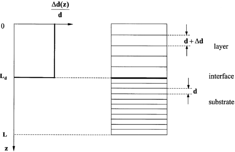
Figure 15: The profile of deformation $(\Delta d(z)/d)$ in a crystal for the bicrystal model. Interplaner distance in the layer $d+\Delta d$ differs from that in the layer on a constant value $\Delta d$. In this model interface is a sharp (step) function located on the depth $L_{d}$.

In this Chapter we will discuss the simplest model of the deformed crystal, so-called bicrystal model, that allows to find analytical solution. In the frame of this model crystal consists of two parts a thick perfect substrate and the deformed layer of thickness $L_{d}$ with the linear dependence of the deformation field $u(z)=(\Delta d/d)z$, where parameter $\Delta d/d$ is a constant difference of the interplanar distance in the layer comparing to that in the substrate (Fig. 15). In this layer parameter $y_{\varphi}(z)=y_{\varphi}=\pi(L_{ex}/d)(\Delta d/d)$ (26) and static Debye-Waller factor $e^{-W(z)}=e^{-W_{0}}$ has constant values. So, in this model deformed layer has a different interplaner distance comparing to that of the perfect substrate. It is additionally partially and uniformly amorphysized and sharp transition (in fact step function) between the layer and the substrate is assumed. Though this model is very simplified it turned out to be very practical in the analysis of the SR yield in a number of experiments.

Analytical solution for the angular dependence of the SR yield $\kappa(\theta)$ and reflectivity $P_{R}(\theta)$ for Bragg diffraction and bicrystal model was obtained for the first time in [51]. This result is a particular case of a more general approach of a multilayer crystal consisting of a number of layers with the different parameters that will be discussed in details in Chapter VII (see also Appendix). According to this approach SR yield for bicrystal model can be obtained from Eq. (132) with the number of the layers $N=2$

$$\kappa_{tot}^{a}(\theta)=\kappa_{L_{d}}^{a}(\theta)+\left|T(L_{d},\theta)\right|^{2}e^{-\mu_{yi}L_{d}}\kappa_{0}^{a}(\theta).$$ (76)

Here, normalized SR yield $\kappa_{tot}^{a}(\theta)$ is a sum of two contributions: from the deformed layer $\kappa_{L_{d}}^{a}(\theta)$ and a perfect substrate $\kappa_{0}^{a}(\theta)$. This functions are defined in Eq.(129) and transmission coefficient $\left|T(L_{d},\theta)\right|^{2}$ can be determined from (122). Deformed layer is characterized by constant values of deformation $\Delta d/d$, static Debye-Waller factor $e^{-W_{0}}$, coherent fraction $F_{c}^{a}$ and coherent position $P_{c}^{a}$. For the perfect substrate $\Delta d/d=0$, $e^{-W_{0}}=1$ and, in general, it can has the values of coherent fraction $F_{c}^{a}$ and coherent position $P_{c}^{a}$ different from that of the layer. The angular dependence of the reflectivity $P_{R}(\theta)$ for Bragg diffraction is obtained from (30) and (114-116) with the amplitude $R_{d_{n}}=R_{0}(\theta)$, where $R_{0}(\theta)$ is the value of the amplitude for the perfect substrate defined in (31).

We want to note here that obtained result is exact and is valid for any relationship between the values of $L_{d}$, $L_{ex}$ and $L_{yi}$. It is also valid for the analysis of the angular dependence of the photoelectron yield or fluorescence radiation in the XSW field. Calculations performed with an exact expression (76) give possibility to take into account minor effects of extinction and variation of phase on the depth of yield of the SR. The convenience of the analytical approach in comparison with the direct numerical calculations lies in the possibility of explicitly separating the dependence on the various parameters.

Essential simplification of Eq. (76) can be obtained in the special case, when the following condition $L_{yi}<<L_{d}<<L_{ex}$ is satisfied. It can be easily fulfilled, for example, for the photoelectron yield. In this case in the angular region of the dynamical diffraction from the substrate $|y(\theta)|<1$ the SR yield (76) can be presented in the following way

$$\kappa(\theta)\approx 1+\beta P_{R}^{id}(\theta)+2\sqrt{\beta}C\left|R_{0}(\theta)\right|F_{c}^{a}(h)\cos\left[\alpha_{Y}(\theta)+\varphi_{h}^{a}+\varphi_{0}\right],$$ (77)

where $P_{R}^{id}(\theta)=|YR_{0}(\theta)|^{2}$ is the reflectivity from a perfect substrate (30–31); $F_{c}^{a}(h)=|Y\varepsilon_{\overline{h}}^{a}|e^{-W_{0}}$ is the coherent fraction; $\alpha_{Y}(\theta)=\alpha(\theta)+\arg(Y)$ where $\alpha(\theta)$ is the argument of the complex amplitude $R_{0}(\theta)$; $\varphi_{h}^{a}=2\pi P_{c}^{a}=\arg(\varepsilon_{\overline{h}}^{a})$, where $P_{c}^{a}$ is the coherent position; and the phase $\varphi_{0}=\varphi(0)=2y_{\varphi}L_{d}/L_{ex}$ gives the total phase shift due to deformation in the layer. In fact this result is a special case of a more general result obtained for the first time in [32] and is valid for any type of deformation if the condition $L_{yi}<<L_{d}<<L_{ex}$ is satisfied.

5.2 Experiment

Now we will show on a number of examples how this theoretical approach can be applied for the analysis of different experiments with the use of XSW for the investigation of the real surface structure.

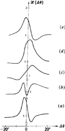
Figure 16: Photoemission angular dependence for $Si$ single crystals with autoepitaxial $Si$ film, doped with $B$ and $Ge$ with varying $Ge$ concentrations: $0$ (curve a), $3.7\times 10^{19}$ (b), $7\times 10^{19}$ (c), $10^{20}$ (d), $1.5\times 10^{20}$ (e). From Ref. [68].

For the first time it was applied for the analysis of homoepitaxial films on Si surface [51] (see also [68]). In this experiments photoelectron yield was measured from a set of specially prepared Si single crystals with the grown homoepitaxial Si films doped with Ge. The concentration of Ge varies from sample to sample from $3.7\times 10^{19}$ to $1.5\times 10^{20}$ atoms $cm^{-3}$. The film thickness was $L_{d}=1.5\mu m$. The $CuK_{\alpha}$ radiation and a (444) non-dispersive double crystal diffraction arrangement with an asymmetric monochromator were used. In this case $L_{yi}=0.45\mu m,$ $L_{ex}=10.5\mu m$ and consequently the condition $L_{yi}<<L_{d}<<L_{ex}$ is fulfilled. The experimental results are presented in Fig. 16. The doping with the Ge atoms changes the plane spacing $\Delta d$ uniformly in the disturbed layer, which leads to a change of the surface displacement. Hence the value of the phase on the surface $\varphi_{0}=|\mathbf{h}|u(0)=2\pi(\Delta d/d)(L_{d}/d)$ also changes. This factor along with the change of Debye-Waller factor $e^{-W_{0}}$ in the surface layer is responsible (according to Eq. (77)) for the variation of the shape of the photoelectron yield curve. Table 1 presents the values of $\varphi_{0}$ and $W_{0}$ obtained by fitting of the experimental curves on Fig. 16 to the theoretical ones calculated using Eq. (77). In this experiment it was demonstrated for the first time high sensitivity of the XSW method for measuring small displacements in the surface layer (in fact, relative difference of the lattice parameter in the layer comparing to that in the substrate). We want to note here, that though lattice parameter changes were comparably not so big from sample to sample the phase difference for high order (444) reflection was of the order of $\pi$ that brought to a significant change of the shape of the curves from sample to sample (see Fig. 16).

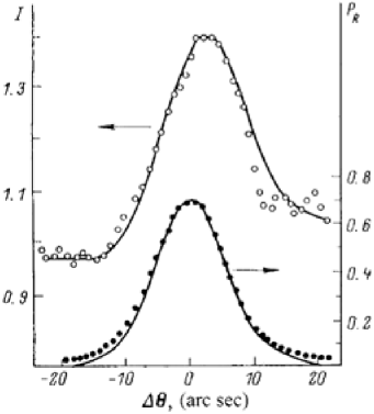
Figure 17: Angular dependence of $InL_{\alpha}$ fluorescence yield from the film of $In_{0.5}Ga_{0.5}P$ (thickness of the film $\sim 100$ Å) grown on the surface of $GaAs$ (111) single crystal (upper curve) and reflectivity (bottom curve). Points are experimental data and lines result of the theoretical fitting. From Ref. [69].

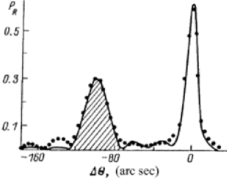
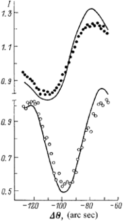
Figure 18: Reflectivity (Top) and angular dependence of $InL_{\alpha}$ (upper curve) and $PK_{\alpha}$ (bottom curve) fluorescence yield (Bottom) from the film of $In_{0.5}Ga_{0.5}P$ (thickness of the film $\sim 0.6$ $\mu m$) grown on the surface of $GaAs$ (111) single crystal. The shadowed region on the reflectivity curve is the region, where angular dependence of the fluorescence yield was measured. Points are experimental data and lines result of the theoretical fitting. From Ref. [69].

In the paper [69] the films of In_0.5Ga_0.5P of different thickness ($\sim 0.01\mu m$ and $\sim 0.6\mu m$ grown on the surface of GaAs (111) single crystal were investigated. The fluorescence radiation from the In and P atoms excited by the XSW field in the substrate (in the case of thin film) and in the film (for thick film) was measured (see Figs. 17, 18).

In the case of thin film condition $L_{yi}=L_{d}<<L_{ex}$ is fulfilled and we can use Eq. (77) to obtain the phase shift $\varphi_{0}$ of the surface layer. Taking also into account relationships (62-64) the angular dependence of the fluorescence yield from the thin film can be analysed from the simple expression,

$$\kappa_{fl}^{a}(\theta)=1+\frac{|E_{h}(\theta)|^{2}}{|E_{0}(\theta)|^{2}}+2C\frac{|E_{h}(\theta)|}{|E_{0}(\theta)|}F_{c}^{a}(h)\cos\left[\alpha(\theta)+\varphi_{h}^{a}+\varphi_{0}\right],$$ (78)

were parameter $F_{c}^{a}(h)$ (coherent fraction) is equal to $F_{c}^{a}(h)=|S_{\overline{h}}^{a}|\exp(-W^{a}(h))F_{0}$, $S_{h}^{a}=|S_{h}^{a}|\exp(i\varphi_{h}^{a})$ is a structure factor of the atoms of the sort $a$, $\alpha(\theta)$ is the phase of the complex ratio $E_{h}/E_{0}$ (see Eq. (38) and $F_{0}=e^{-W_{0}}$ is the average amorphization of the surface layer.

From the fitting of the experimental curve to the theoretical one (Eq. (78)) it was obtained the value of $F_{0}=0.25$ and of the phase shift $\varphi_{0}=0.55$ that correspond to the average deformation in the film $\Delta d/d\approx 6\cdot 10^{-3}$. The same approach was used in [70] for the analysis of the film In_xGa_1-xAs_yP_1-y grown on the substrate InP (100). Small deformation $\Delta d/d\approx 2.3\cdot 10^{-4}$ in a thicker film $L_{d}\approx 0.2\mu m$ was measured with XSW method.

In the case of the thick film x-ray standing wave field is formed in the film itself. Fluorescence yield measured in the angular position of the film maximum has different behavior for In and P atoms due to different position of the atoms in the unit cell. In this case the simplified approach of Eq. (78) is not valid any more and general approach based on Eq. (76) was used for fitting (see Fig. 18). As a result thickness of the film $L_{d}=0.62\mu m$, deformation $\Delta d/d\approx 2\cdot 10^{-3}$ and amorphization factor $F_{0}=0.8$ were obtained. However as it is seen from Fig. 18(b) coincidence between the experimental and theoretical curves is not perfect, that can be due to simplified bicrystal model, that does not take into account transition layer between the film and the substrate. In this situation the theoretical model with transition layer proposed in [71] can be useful for the analysis of the angular dependence of the fluorescence yield from the geterostructures.

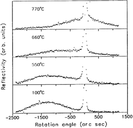
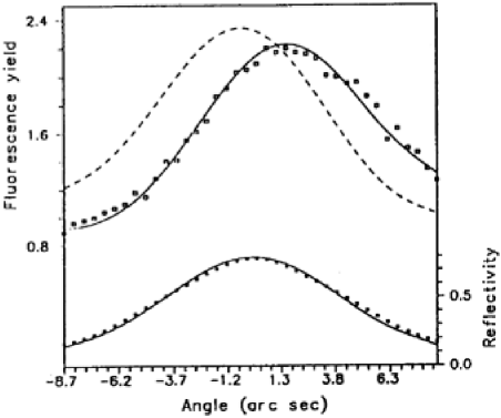
Figure 19: (Left:) The (222) x-ray reflectivity curves of $CaF_{2}$ epitaxial $10$ nm layers grown at different temperatures; (Right:) Angular dependence of the total photoelectron yield $\kappa$ (upper curve) and reflectivity $P_{R}$ (bottom curve) for the (888) diffraction of $CuK_{\alpha}$ radiation in a perfect GGG garnet single crystal. Points are experimental data and lines are theoretical fitting. From Ref. [74].

Thin epitaxial films of CaF₂ grown on Si (111) surface where characterized by impurity luminescence probes, x-ray diffractometry and x-ray standing wave technique [72, 73]. Molecular beam epitaxy was used to grow 10nm thick films. The CaF₂/Si interface was formed at $770^{\circ}C$. Due to different growth conditions strain field in each CaF₂ film is different. This is well seen from the reflectivity (222) curves measured from the different samples (Fig. 19(a)). The angular dependence of the CaK_α fluorescence excited by the XSW field in the Si (111) substrate was also measured (Fig. 19(b)). In this case we again have the situation, when $L_{yi}=L_{d}<<L_{ex},$ and expression (78) can be applied for the analysis. Finally the strain field in the film was obtained independently from the photoluminescence study and x-ray rocking curve analysis and are summarized in the Table 2. X-ray standing wave analysis gave an additional information: the distance between the first (as counted from the substrate) atomic plane of the film and the diffracting plane of the substrate nearest to the interface (denoted as $P^{hkl}$) and the static Debye-Waller factor $e^{-W_{0}}$ of the film.

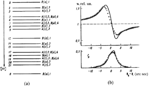
Figure 20: (a) Schematic arrangement of the planes consisting from the different sort of atoms in positions a, c and d in a single garnet crystal in the direction [111] in the unit cell; (b) Angular dependence of the total photoelectron yield $\kappa$ (upper curve) and reflectivity $P_{R}$ (bottom curve) for the (888) diffraction of $CuK_{\alpha}$ radiation in a perfect GGG garnet single crystal. Points are experimental data and lines are theoretical fitting. From Ref. [74].

Comprehensive study of different type of garnet crystals with different kind of films on the surface were analysed with XSW method monitoring photoelectron yield and fluorescence radiation in [74, 75, 76] (first measurements of fluorescence radiation from garnet single crystals were performed in [63]). Peculiarity of the garnet crystals is a comparably complicated unit cell containing 160 atoms (for the distribution of different atoms in the unit cell of garnet crystal in the (111) direction see Fig. 20(a)). Another interesting property is that due to the fact, that garnet crystals contain heavy atoms with $Z>>1$ propagation of x-rays in this crystals is highly reduced and fluorescence yield from this atoms is absorbed on a short distances of about $1\div 10\mu m$.

The angular dependence of the total photoelectron yield from the gallium gadolinium garnet (GGG) crystals excited by the XSW field was measured for the first time in [74] (Fig. 20(b)). Due to a small value of the absorption depth $L_{0}=\sin\theta_{B}/\mu_{0}=5.44\mu m$, that is comparable with the extinction length $L_{ex}=3.88\mu m$ in this crystal the reflection coefficient for (888) diffraction of CuK_α radiation has a small $\sim 47\%$ maximum value. At the same time the photoelectron yield curve has a phase sensitive dispersion like shape.

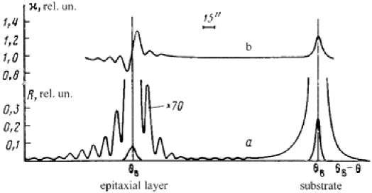
Figure 21: Experimental results of the photoelectron yield $\kappa$ (upper curve) and reflectivity $P_{R}$ (bottom curve) for (888) diffraction of $CuK_{\alpha}$ radiation in a perfect GGG garnet crystal with an epitaxial film of FYG garnet crystal with the thickness 2 $\mu m$. From Ref. [74].

In the same paper the angular dependence of the photoelectron yield for the GGG crystal with the epitaxial film (thickness of the film $L_{d}=2\mu m$) of the iron yttrium garnet (FYG) was measured (Fig. 21). The same CuK_α radiation and (888) reflection as in the previous case was used. For the theoretical description of the photoelectron yield in this case of thick film the general theory of bicrystal model described in the first part of this chapter can be applied. However for understanding the physics of formation of the photoelectron yield while the dynamical diffraction some simplified considerations can be used. Lattice parameters of the FYG film and of the GGG substrate does not differ essentially (the same is valid for their Bragg angles), however the Fourier components of the susceptibility $\chi_{h}$ are quite different. For example, extinction depth for the FYG crystal is equal to L${}_{ex}=5.68$ $\mu m$ that is essentially bigger then the thickness of the film ($L_{d}<<L_{ex}$), so reflection from the film is kinematical. In the kinematic approximation we have for the reflectivity,

$$P_{R}(\theta)=\frac{C_{p}}{y^{2}(\theta)}\sin^{2}\left[\frac{L_{d}}{L_{ex}}y(\theta)\right],$$ (79)

where angular deviation parameter $y(\theta)$ is defined in (25) and $C_{p}=(1+C^{3})/(1+C)$ is the polarization factor. In this approximation we have for the photoelectron yield,

$$\kappa_{ph}(\theta)=1+K\sin^{2}\left[\frac{L_{d}}{L_{ex}}y(\theta)\right]\left[-\frac{2}{y(\theta)}\mid\varepsilon_{\overline{h}}\mid+\frac{1}{y^{2}(\theta)}\right].$$ (80)

Parameters in equations (79-80) in the case of experiment [74] has the following values $K=0.75,\mid\varepsilon_{\overline{h}}\mid=0.8$ and we obtain for $P_{R\max}=0.092,$ $\kappa_{\min}=0.75,$ $\kappa_{\max}=1.33.$ This simple approximation fit quite well to the experiment. At the same time the photoelectron yield at the angular position of the substrate peak has the shape similar to the reflectivity curve (this is quite similar to the discussed before case of amorphous layer, however the physics of the process is different). Period of the standing wave formed in the substrate is different from that of the film (measured photoelectrons are excited only in the film). Due to this difference there is no correlation between the positions of the atomic planes on the escape depth of the electrons and the positions of the nodes and antinodes of the standing wave. In this experiment the escape depth of the electrons is about of $L_{yi}=0.22$ $\mu m$. On this depth due to the difference in the period of the film lattice and the substrate atom is shifted on $1.44\AA$ and at the same time the period of the standing wave for (888) reflection is equal to $a\sqrt{3}/24=0.89\AA.$ Finally, due to a big variation of phase on the period of the standing wave field the third term in the expression for the photoelectron yield $\kappa_{ph}(\theta)$ (77) cancel out and we obtain for $\kappa_{ph}(\theta)=1+P_{R}(\theta).$

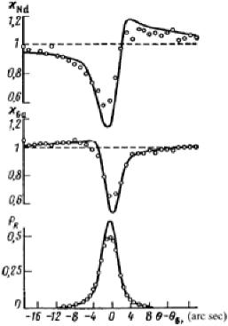
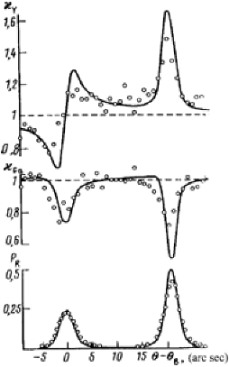
Figure 22: (Left:) Angular dependence of the fluorescence yield of $NdL_{\alpha}$ (upper curve) and $GaK_{\alpha}$ (middle curve) for the (444) diffraction of $MoK_{\alpha}$ radiation (reflectivity is shown on the bottom curve) for the perfect GNG garnet crystal; (Right:) Angular dependence of the $YK_{\alpha}$ fluorescence yield from the film (upper curve) and $GaK_{\alpha}$ fluorescence yield from the substrate (middle curve) for the (444) diffraction of $AgK_{\alpha}$ radiation (reflectivity is shown on the bottom curve) for the perfect GGG garnet crystal with an epitaxial film of FYG crystal with the thickness 1.6 $\mu m$. Points are experimental data and lines are theoretical fitting. From Ref. [74].

In the same paper the fluorescence yield from the Gallium-Neodymium Garnet (GNG) crystal and the films of FYG (thickness of the film $L=1.6\mu m$) on the top of GGG crystal with XSW method were investigated. Due to a big depth of yield of the fluorescence radiation ($L_{yi}^{Ga}=20.4\mu m$ for GaK_α radiation and $L_{yi}^{Nd}=15.1\mu m$ for NdL_α radiation) comparing to the extinction length ($L_{ex}=1.54\mu m$) the angular dependence of the fluorescence yield curves in the XSW field is determined by extinction effect discussed in the section 4.1. However as we can see from Fig. 22(a) the fluorescence yield from Nd and Ga atoms has different asymmetry on the tails of the curves. This is due to the fact, that for reflection (444) the phase of the standing wave on the neighbour atomic layers (on the distance of $1/24$ of the period) differs by $\pi.$ At the same time average coherent positions for Ga and Nd atoms coincide, but the effective coherent fractions $F_{c}$ are different: $F_{c}^{Ga}=0.321$ and $F_{c}^{Nd}=1.628$.

For the theoretical analysis of the fluorescence yield curves from the FYG films on the GGG crystal substrate the bicrystal model described in this section was used. While fitting in this case it was additionally taken into account the change of the susceptibility of the film $\chi_{film}$ comparing to that of the substrate $\chi_{substrate}$ as well as the change of the interplanar distance $\Delta d/d.$ Results of the fitting are presented on Fig. 22(b). In this case YK_α fluorescence radiation from the atoms of the film and GaK_α radiation from the atoms of the substrate in the case of (444) diffraction of AgK_α radiation were measured. Different shape of the curves reflects different conditions of the fluorescence yield formation in XSW field. Extinction depth is equal to $L_{ex}=2.3\mu m$ and is bigger then the thickness of the film. The depth of yield of the YK_α radiation is restricted by the thickness of the film and coincide with the volume of XSW formation in the film (the same as on Fig. 21, but with bigger value of $L_{d}/L_{ex}$). At the same time (when Bragg conditions for the film are fulfilled) the Ga fluorescence yield is decreased because x-rays being reflected in the film hardly penetrate to the substrate, where Ga atoms are located. Right maximum on the reflectivity curve on Fig. 22(b) correspond to the reflection of x-rays from the substrate. In this case the angular dependence of the GaK_α fluorescence yield has a big dip due to an extinction effect described before (due to a big escape depth of the fluorescence radiation comparing to an extinction depth). At the same time the yield of the YK_α radiation in this angular region has a maximum of the same origin as described on Fig. 21.

In the papers [75, 76] XSW method was used to study the positions of $Bi^{3+}$ ions in the lattice of a heteroepitaxial film of yttrium-bismuth iron ($Y_{3-x}Bi_{x}Fe_{5}O_{12}$) garnet. The main problem was to determine quantitatively the distribution of bismuth over the different dodecahedral positions which are occupied by yttrium in a pure yttrium iron garnet. This information is essential for understanding the growth-induced magnetic anisotropy of this garnet crystals. The stated problem was solved by detailed analysis of the angular dependence of the $Bi^{3+}$ fluorescence.

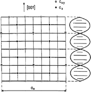
Figure 23: Projection of the dodecahedral positions $c_{z}$ (full circles) and $c_{xy}$ (open circles) on the plane (001). The (004) x-ray standing wave is also shown schematically. From Ref. [76].

Ideal garnets have cubic symmetry with cations entering octahedral (a), tetrahedral (d) and dodecahedral (c) sublattices. In the $Y_{3-x}Bi_{x}Fe_{5}O_{12}$ system $Bi^{3+}$ and $Y^{3+}$ ions enter only the $c$ sites. For the [001] growth direction there are two inequivalent groups of dodecahedral sites, the first consists of 16 sites, which are denoted as $c_{xy}$, the second consists of 8 sites denoted as $c_{z}$ [77]. The distribution of $c_{xy}$ and $c_{z}$ sites within the elementary cell for this growth direction together with the distribution of the nodes and antinodes of (004) X-ray standing wave is shown in Fig. 23. Note that the sites belonging to the $c_{xy}$ and $c_{z}$ groups lie in different layers and consequently they can be, in principle, distinguished by the XSW method.

For the analysis of the fluorescence yield from this garnet samples a bicrystal model consisting of the thin film and the substrate was used. If the depth of yield of the fluorescence radiation $L_{yi}$ is much smaller than the extinction length $L_{ex}$ the angular dependence of the intensity of fluorescence radiation in multicomponent crystal is given by Eq. (78). For the reflection (004) the inequivalent groups of sites $c_{z}$ and $c_{xy}$ have different structure factors $S_{h}(c_{z})=-1$ (8 sites), $S_{h}(c_{xy})=+1$ (16 sites). The structure factor of the $Bi^{3+}$ ions, which enter the dodecahedral sublattice in $Y_{3-x}Bi_{x}Fe_{5}O_{12}$ garnet films, is influenced by the distribution of these ions between $c_{z}$ and $c_{xy}$ positions. The fraction of $Bi^{3+}$ ions in $c_{z}$ positions will be denoted by parameter $p$

$$p=\frac{N_{z}^{Bi}}{N_{z}^{Bi}+N_{xy}^{Bi}},$$

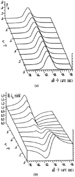
Figure 24: Calculated angular dependencies of the reflectivity $P_{R}(\theta)$ (a) and fluorescence yield of the $Bi$ (b) for the (004) diffraction of $MoK_{\alpha}$ radiation on $Y_{3-x}Bi_{x}Fe_{5}O_{12}$ thin film for the values of $p$ from 0 to 1 in the angular range of the x-ray diffraction on the film. From Ref. [76].

where $N_{z}^{Bi}$, $N_{xy}^{Bi}$ are the numbers of $Bi^{3+}$ ions in $c_{z}$ and $c_{xy}$ sites, respectively. Then the structure factor of $Bi^{3+}$ ions for the (004) reflection is $S_{h}^{Bi}=1-2p$ and due to Eq. (78) the fluorescence yield of $Bi^{3+}$ ions will depend on the value of the parameter $p$. The uniform distribution of $Bi^{3+}$ ions between $c_{z}$ and $c_{xy}$ sites corresponds to $p=1/3$. The calculated angular curves of the reflectivity and $Bi^{3+}$-ion fluorescence yield for values of $p$ in the interval $0$ to $1$ are shown in Fig. 24. The angular yield curves of the $Bi^{3+}$ fluorescence demonstrate, as expected, a strong dependence on the distribution of these ions. For values of the parameter $p=0$ (all $Bi^{3+}$ ions in $c_{xy}$ sites) and $p=1$ (all $Bi^{3+}$ ions in $c_{z}$ sites) the amplitude of the structure factor of the $Bi^{3+}$ ions attains its maximum ($\left|S_{h}^{Bi}\right|=1$) and the phase $\varphi_{h}^{Bi}$ of the structure factor equals $0$ and $\pi$, respectively. The angular yield curves for these limiting cases show reversed positions for maxima and minima of the yield. When $\left|S_{h}^{Bi}\right|$ decreases the ratio of the fluorescence to the background becomes smaller. Note that on the curve corresponding to $p=0.33$ (uniform distribution of $Bi^{3+}$ ions over $c_{z}$ and $c_{xy}$ sites) a clear maximum occurs at the high-angle side (with respect to the maximum of Bragg diffraction on the film). At the same time the reflectivity curves (Fig. 24(a)) has very small dependence on the value of the parameter $p$.

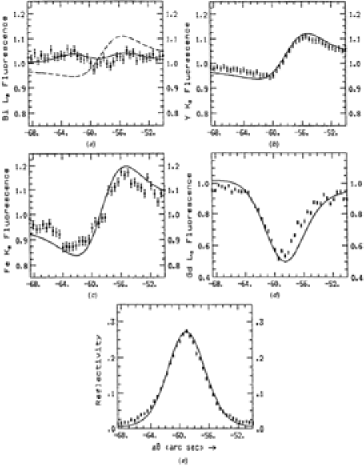
Figure 26: Experimental (points) and calculated (lines) for the value of $p=0.44$ angular dependencies of the fluorescence yield of $Bi^{3+}$ (a), $Y^{3+}$ (b), $Fe^{3+}$ (c) ions from the film and $Gd^{3+}$ ions from the substrate (d) and the x-ray reflectivity (e). For comparison the fluorescence yield curve for $p=0.33$ (uniform distribution of $Bi^{3+}$ ions over $c_{z}$ and $c_{xy}$ sites) is also shown in (a). From Ref. [76].

The diffraction curve for the sample studied is shown in Fig. 25. The angular distance between two peaks (corresponding to the substrate and the film) allows a direct determination of the lattice mismatch between the film and substrate $\Delta d/d=2.5\times 10^{-3}$. In Fig. 26 the experimental angular dependencies of the fluorescence of $Bi^{3+}$ (Fig. 26(a)), $Y^{3+}$ (Fig. 26(b)), $Fe^{3+}$ (Fig. 26(c)) and $Gd^{3+}$ (Fig. 26(c)) are shown together with the reflectivity curve (Fig. 26(e)) in the angular range corresponding to the diffraction on the film. Results can be understood on the basis of the theory described in the first part of this Chapter. Three main factors influence the shape of the fluorescence yield curve, namely the amplitude and the phase of the structure factor of the sublattice of the ions under study and the extinction effect for a given thickness of the film. The experimentally observed shape of the curve is determined by the fact that the $Bi^{3+}$ sublattice structure factor is close to zero and the extinction effect for a given thickness of film leads to the decrease of intensity. The best fit (shown on Fig. 26 by solid curve) was obtained for the following values of the parameter $p=0.44\pm 0.02$, thickness of the film $L_{d}=3\mu m$, and Debye-Waller factors of the film and the substrate $\exp(-W_{f})=\exp(-W_{s})=0.93$. Small mosaicity of the sample is also taken into account by additional convolution of the calculated curves with the Gaussian function with $\sigma=3.8\mbox{ arcsec}$. The obtained value of the parameter $p$ represents the main result of the papers [75, 76]. Due to interference nature of the XSW method it gives the possibility to obtain the value of this parameter with high accuracy (see Fig. 26a), where $Bi^{3+}$ fluorescence yield curve with the value of $p=0.33$ corresponding to the uniform distribution of $Bi^{3+}$ ions) is also shown for comparison.

The same bicrystal model was used in the analysis of a recent experiment [78] where the lattice constant difference of the isotopically pure ${}^{76}Ge$ grown as a film on the top of a natural $Ge$ single crystal was measured as a function of the temperature. The variation of XSW in the film was monitored with the photoelectron detector.

6 XSW in Laue geometry

Up to now we were considering formation of Standing Waves in crystal and secondary radiation yield for the Bragg geometry of diffraction. Registration of SR yield in Laue geometry has it’s own peculiarities different from Bragg geometry of scattering and will be discussed in this Chapter. XSW in the Laue case with the registration of SR yield from the exit surface have been studied in several papers concerning lattice-atom fluorescence yield [79], external [80] and internal [18] photoeffect. A Laue-case interferometer was used for the location of chemisorbed atoms [81]. In this Chapter we will present mainly theoretical and experimental results obtained in [82, 83], where the formation of the fluorescence-yield angular curves in the Laue case and the possibilities of this geometry for the location of impurity atoms were studied. The advantage of the Laue geometry of diffraction (Fig.19) is the possibility to study the position of impurity atoms distributed through the bulk of a crystal. In this case the sensitivity of XSW in the Bragg geometry decreases due to extinction effect (see discussion in Chapter 4 of this review). Moreover, in the Laue case it is easy to use different reflections (including asymmetrical ones) to study the impurity-atom positions in different crystallographic directions.

6.1 Theory

The general theory of SR yield described in Chapter 3 is valid for the Laue geometry as well. The yield of the SR is determined by the expression similar to (52)

$$\kappa^{a}(\theta) = \frac{1}{I(\infty)}\int\limits_{0}^{L}dzP_{yi}^{a}(z)\left\{\left|E_{0}(z,\theta)\right|^{2}+\left|E_{h}(z,\theta)\right|^{2}+\right.$$ (81)

$$\ \ \left.+2CF_{c}^{a}(z)Re\left[E_{0}^{*}(z,\theta)E_{h}(z,\theta)\exp[i\varphi^{a}(z)]\right]\right\},$$

where

$$F_{c}^{a}(z)=e^{-W^{a}(z)}|\varepsilon_{\overline{h}}^{a}|$$ (82)

is coherent fraction and $L$ is the crystal thickness. The type of the SR and the type of atoms emitting it are characterized by index $a$. The phase $\varphi^{a}(z)=2\pi P_{c}^{a}+\mathbf{hu}(z)=\varphi_{\overline{h}}^{a}+\mathbf{hu}(z)$ and the factor $\exp[-W^{a}(z)]$ correspond only to the atoms of type $a$, $\varphi_{\overline{h}}^{a}=2\pi P_{c}^{a}$ is the phase of the complex value $\varepsilon_{\overline{h}}^{a}$ (62) and $P_{c}^{a}$ is coherent position. The function $P_{yi}^{a}(z)$ describes the yield of SR emitted by atoms of type $a$ located at depth $z$. In the case of Laue geometry and the fluorescence yield from the exit surface $P_{yi}^{a}(z)=c_{a}\exp[\mu_{yi}^{eff}(z-L)]$, where $\mu_{yi}^{eff}=1/(\gamma_{fl}L_{yi}^{fl})$, $L_{yi}^{fl}$ is the depth of the fluorescence yield, $c_{a}$ is the concentration of the impurity atoms (see Eq. (55)).

The field amplitudes $E_{0s}(z,\theta)$ and $E_{hs}(z,\theta)$ for the crystal with the deformation field $\mathbf{u}(z)$ and Laue geometry of diffraction (in this case parameter $\gamma_{h}>0$) can be obtained from the general TT equations (18). In this Chapter it will be discussed in details the situation, when crystal can be considered as a set of two layers (bicrystal model) with different lattice parameters, perfection and atomic compositions. A crystal lattice of each layer is characterized by a constant value of the parameters $\Delta d/d$, $\exp(-W)$ and $\chi_{0,h},$ which describe the change of the plane spacing, decrease of the coherent scattering amplitude and the composition, respectively.

Let us consider like in the previous Chapter a layer of thickness $L_{d}$ at the depth $z_{0}<z<z_{0}+L_{d}$. The phase $\varphi(z)$ in (18) depends linearly on $z$ because $\Delta d/d$ is a constant within a layer

$$\varphi(z)=\varphi(z_{0})+2y_{\varphi}\Delta z/\overline{L}_{ex},$$ (83)

where $\Delta z=z-z_{0}$, $y_{\varphi}$ and $\overline{L}_{ex}$ are constant, $\overline{L}_{ex}$ is an extinction length averaged over the crystal bulk. The solution of TT equations (18) should satisfy the given values of $E_{0s}(z,\theta)$ and $E_{hs}(z,\theta)$ on the entrance boundary of the layer.

As it was shown in Chapter 2, if the amplitude function $R(z,\theta)$ is defined in the form (23), then it satisfies non-linear equation (24) (for Laue case lower signs has to be taken) with a boundary condition $R=R_{0}$ on the upper boundary of a layer at $z=z_{0}$. The solution of Eq. (24) in the Laue geometry with constant parameters can be found analytically (see Eq. (114) from Appendix, where in the case of one layer the value of $R_{n}$ on the upper boundary has to be changed by $R_{0}$). Intensity of the transmitted beam $I_{0}(z,\theta)=\left|E_{0}(z,\theta)\right|^{2}$ on the depth $z$ defined in (34) also can be found analytically (see Eqs. (120-123) from Appendix).

The contribution of the layer with the thickness $L_{d}$ to the SR yield in the frame of these model is analysed in details in Appendix and is summarized in Eqs. (129-131), where thickness of the layer $d_{n}$ has to be changed by $L_{d}$. This equations have to be complemented by the boundary conditions on the entrance surface of crystal, where $E_{0}=1$ and $R=0$. X-ray transmission ($P_{T}(\theta)$) and reflectivity ($P_{R}(\theta)$) are given by

$$P_{T}(\theta)=\left|E_{0}(L,\theta)\right|^{2},P_{R}(\theta)=P_{T}(\theta)\left|YR(L,\theta)\right|^{2}.$$ (84)

Finally the problem of the SR yield from the exit surface of the crystal in Laue geometry is completely defined. If measurements are made in a double-crystal scheme with the first crystal-monochromator convolution with the first crystal reflectivity curve (according to (53)) has to be taken into account.

6.2 Experiment

Theory of the SR yield in Laue geometry of diffraction described in the previous subsection was applied in [82, 83] for the analysis of the experimental results.

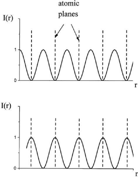
Figure 27: (Top:) Experimental set up for SR yield measurement in Laue geometry: $C_{1}$ crystal monochromator, $C_{2}$ crystal under investigation, $NaI$ detector measuring reflectivity, $Si(Li)$ detector measuring fluorescence yield. (Bottom:) Distribution of x-ray standing wave field in a crystal for Laue geometry. Nodes of the weakly absorbing field (upper curve) coincide with the atomic planes and maximum of field intensity for highly absorbing (bottom curve) coincide with atomic planes giving maximum absorption of this field on the thickness of the crystal $L$.

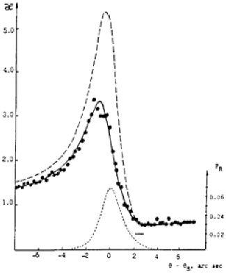
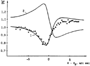
Figure 28: Angular dependence of the $GeK_{\alpha}$ fluorescence yield from the $Si$ crystal uniformly doped with $Ge$ with different thickness of the crystal. Points are experimental data, lines are calculations. (Left:) Case of the thick crystal ($L=2.2$ $mm$). Solid line is the calculation for substitutional impurity atoms (coherent position $P_{c}^{111}=0$); dashed curve is the calculation for impurities with coherent position $P_{c}^{111}=0.15$. The x-ray reflectivity curve $P_{R}$ is also shown. (Right:) Case of the thin crystal ($L=0.49$ $mm$). Curve 1 is the calculation for the substitutional impurity atoms and curve 2 is the calculations for the randomly distributed impurities. From Ref. [83].

In the first series of measurements $Si$ single crystals of different thickness with (100) surface orientation uniformly doped during growth with germanium ($N_{Ge}=7.5\times 10^{25}$ $m^{-3}$) were used. $GeK_{\alpha}$ fluorescence from the exit surface of the silicon crystals in the Laue geometry and (111) reflection was measured by an energy-dispersive $Si(Li)$ detector (see Fig. 27). The angular dependence of $GeK_{\alpha}$ fluorescence yield from a thick crystal with thickness $2.2$ $mm$ (Fig. 28a) shows a large maximum slightly shifted to the low-angle side with respect to the maximum of the diffracted intensity. On the contrary, in the case of a thin crystal with thickness $0.49$ $mm$, the fluorescence curve (Fig. 28b) shows a dip near the center of the reflection range and a weak maximum at the high-angle side.

According to our previous theoretical approach in this case the whole crystal can be considered as one layer with thickness $L_{d}=L$ and fluorescence yield can be determined by Eq. (129). In experiments the following conditions were also fulfilled $L_{0}>>L_{yi}>>L_{ex}$, where $L_{0}=\gamma_{0}/\mu_{0}$. Since $L_{yi}>>L_{ex}$, the third (interference) term in (129) is very small ($\left|\psi_{3}\right|<<\left|\psi_{1}\right|\left|\psi_{2}\right|$) and can be neglected. On the other hand, since $L_{0}>>L_{yi}$ the normalized fluorescence yield does not depend on $L_{ex}$ and $L_{yi}$. Taking this considerations into account from (129) an approximate expression can be obtained

$$\kappa(L,\theta)\simeq\sum\limits_{k=1,2}I_{k}(\theta)\exp\left[\Delta\mu_{k}(\theta)L\right],$$ (85)

where

$$I_{k}(\theta) = \frac{1+\beta x_{k}^{2}+Bx_{k}}{1+x_{k}^{2}},$$

$$x_{1,2} = \left[-y\mp\sqrt{y^{2}+C^{2}}\right]\left/C\right.,$$

$$\Delta\mu_{k}(\theta) = -x_{k}\frac{\left[2C\sqrt{\beta}\left|\varepsilon_{\overline{h}}\right|/\chi_{0i}-x_{k}(1-\beta)\right]}{L_{0}(1+x_{k}^{2})},$$ (86)

$$B = 2C\sqrt{\cdot\beta}\varepsilon_{h}^{a}\exp(-W^{a})\cos(2\pi P_{c}^{a}).$$

To derive (85) the following values of the parameters were used $Y=1,$ $y_{\varphi}=0$ and expansion for the complex parameters $x_{k}$ in the power series of a small value $\chi_{i}/\chi_{r}$ were used.

The most significant feature of Laue-case X-ray diffraction is that two types of standing waves are formed in a crystal (Fig. 27b). One of these waves is a weakly absorbed field with the nodes on the atomic planes, corresponding to the well known Borrmann effect. The other one is a strongly absorbed field with the antinodes on the atomic planes. So, as follows from (85), the fluorescence yield angular curve differs distinguishably for a thick crystal ($L>>L_{0}$) and a thin one ($L<L_{0}$). The experimental curve shown in Fig. 28a corresponds to $L=4.3L_{0}$. In this case the SR yield is excited only by the weakly absorbed X-ray standing wave field [$k=1$ in (85)]. The other feature of the Laue case is that with rocking a crystal through the reflection position, the standing wave fields do not move with respect to the atomic planes (as in the Bragg case), but only intensities of these fields increase or decrease. The weakly absorbed field has a maximum intensity at $\theta=\theta_{B}$. Even for impurity atoms lying strictly in the crystal nodes ($P_{c}^{a}=0$) one can observe an increase of the fluorescence yield at $\theta\simeq\theta_{B}$ in comparison with a background yield. At any displacement from the crystal node, the impurity atom occurs in the region of the increased field intensity and fluorescence yield increases even more.

The obtained experimental curve (Fig.20a) is in a good agreement with the theoretical one for the model of substitutional impurity atom position. The maximum normalized fluorescence yield is equal to $3.3$. For the impurity atom between the reflecting planes ($P_{c}^{a}=0.5$) this value will be $13.9$. Note, that the sensitivity to the position of the impurity atom increases with increasing crystal thickness. Calculated dependencies of the normalized fluorescence yield maximum on the impurity position with respect to (111) and (022) reflecting planes are shown in Fig. 29 for different crystal thickness. Crystals with intermediate thicknesses are more appropriate for impurity location studies, due to a rapid decrease of the background fluorescence yield with increasing of crystal thickness. It should be noted that a randomly distributed fraction of impurities also leads to an increase of the fluorescence yield. Indeed, the static Debye-Waller factor for impurity atoms $\exp(-W^{a})$ and the term $\cos(2\pi P_{c}^{a})$ describing coherent displacements are included in (85) as the multipliers.

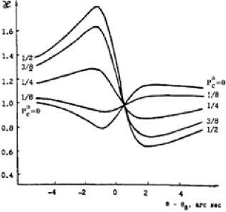
Figure 30: Calculated angular dependencies of the impurity fluorescence yield from a thin $Si$ crystal for a different impurity positions. From Ref. [83].

For a thin crystal, because of the excitation of both standing wave fields the situation is more complicated. Both weakly ($k=1$) and strongly ($k=2$) absorbed fields can make a significant contribution to the fluorescence yield curve, but at different angular positions: field $1$ at $\theta<\theta_{B}$ and field $2$ at $\theta>\theta_{B}$. The main factor now is a degree of interaction of impurity atoms with the standing wave fields but not the anomalous X-ray transmission. If the impurity atom is located on diffraction plane, it interacts with field $2$ more than with field $1$. So, the maximum of the yield will be observed at $\theta>\theta_{B}$ (curve $1$ in Fig. 28b). The minimum on curve 1 occurs because field 1 does not interact with impurities and field 2 is not excited in this angular region. If impurity atoms are randomly distributed [in (86), $\exp(-W^{a})=B=0$], this effect is compensated entirely by increasing the interaction with field 1 (curve 2 in Fig. 28b). In Fig. 30, one can see the fluorescence yield curves calculated for different positions ($P_{c}^{a}$) of impurity atoms. It is obvious that with displacement of the impurity from the diffraction plane interaction with the weakly absorbed field increases and with the strongly absorbed field decreases. So, the fluorescence yield increases at $\theta<\theta_{B}$ and decreases at $\theta>\theta_{B}$. The experimental curves both for thick and thin crystals unambiguously show that germanium is substitutional in silicon. Such behavior corresponds to the isovalent nature of this impurity.

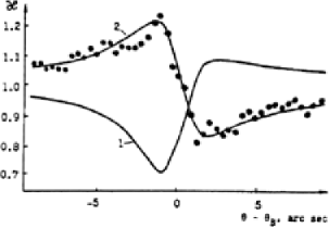
Figure 31: Angular dependence of the $GeK_{\alpha}$ fluorescence yield from the $Si$ crystals with an epitaxial layer with thickness $0.35$ $mm$. (Left) Angular region corresponding to the x-ray diffraction on the substrate. Curve 1 is the calculation for the substitutional impurity atoms; curve 2 is the calculation for the randomly distributed impurities; circles are the experimental data. (Right) Angular region corresponding to the x-ray diffraction on the layer. Fluorescence yield is presented on the upper curve and reflectivity on the bottom. Dashed lines are calculations for substitutional impurity atoms (1) and for the randomly distributed impurities (2). From Ref. [83].

In the second series of measurements $Si$ crystals with thickness $0.35$ $mm$, (111) surface orientation with an epitaxial layer with thickness $1.6$ $\mu m$ on the exit surface were studied. During growth the epilayer was doped with boron and simultaneously with germanium ($N_{Ge}=10^{28}$ $m^{-3}$). The experimental curve of $GeK_{\alpha}$ fluorescence yield from the epilayer in the angular range of diffraction in the substrate is shown in Fig. 31a. In this case fluorescence was excited by XSW formed in the bulk of the crystal. An X-ray rocking curve in a wide angular range is shown in Fig. 31b. From this rocking curve the deformation in the epilayer comparing to that in the substrate can be estimated as $\Delta d/d=-3.8\times 10^{-3}$. In the conditions of X-ray diffraction on the epilayer, the so-called ’kinematical’ standing waves are formed in this layer. The fluorescence yield in this angular range is shown in Fig. 31b. Weak minimum and maximum were clearly observed on the increasing background. The angular dependence of the background is due to the difference between the plane wave and the wave incident on the layer due to the diffraction in the bulk.

In this series of experiments the layer with thickness $L_{d}=1.6$ $\mu m$ is much less than the extinction length $L_{ex}=12.6$ $\mu m$ and $L>L_{0}$. Impurity atoms which are only in the layer ’see’ both standing wave fields and their interference in the angular range of the X-ray diffraction in the substrate. The interference term oscillates with increasing $z$ and the period of these oscillations is different at different values of the incident angle: at $\theta=\theta_{B}$ the period is equal to $\pi L_{ex}$ and it decreases with increasing $|\theta-\theta_{B}|$. Since $L>>L_{ex}$, the fluorescence yield angular curve for the case of the incident plane wave strongly oscillates with the period less than the angular divergence of the real incident beam. So, in the treatment of the experimental curve the interference term can be averaged again giving a zero contribution, although the reason for this averaging is quite different for that of the previous case.

Taking all this into account, it is clear why the calculated curves in Fig. 31a for substitutional and randomly distributed impurities are very similar to the curves in Fig. 28b, although the calculations were carried out in a double-layer model including convolution. In this case opposite to the previous one the experimental curve is in a good agreement with the model of random distribution. This means that impurity atoms are in all possible positions with respect to the standing waves formed in the substrate. Nevertheless, impurities in the layer could be ordered, but with period different from the period of the substrate reflection planes.

The problem of the impurity position can be solved by measuring the fluorescence yield curve in the angular range of X-ray diffraction on the epilayer. Since the reflection of X-rays by the epilayer is small ($L_{d}<<L_{ex}$), the standing wave formed in the layer has the intensity weakly oscillating around the average value. It is the case of so-called kinematical standing waves. The total reflectivity amplitude $R(z,\theta)$ (23) in the kinematical approximation can be presented in the following form

$$R(z,\theta) = Ce^{-W}e^{iqz}\frac{\sin(qz)}{iqL_{ex}}+$$

$$\ R_{0}(\Delta\theta+\Delta\theta_{B})e^{2iqz},$$

where the coordinate $z$ starts from the upper boundary, $q=y/L_{ex}=(\pi\sin 2\theta_{B}/\lambda\gamma_{h})\Delta\theta$, $\Delta\theta=\theta-\theta_{B}$ is the angular deviation from the Bragg angle for the layer, $\Delta\theta_{B}=\theta_{B}-\theta_{B}^{0}$, where $\theta_{B}$ and $\theta_{B}^{0}$ are the Bragg angles for the layer and the substrate, $R_{0}$ is the reflectivity amplitude of the substrate.

The fluorescence yield from the layer is defined by the general equation (81) but at $L_{yi}>>L_{d}$ one can put $P_{yi}^{a}(z)=1$ in (81). Moreover, one can consider that the amplitude of the ’incident’ wave does not depend on $z$ and this is the $0$ component of one of the standing waves formed in the substrate. Since X-ray diffraction by the layer is observed at $\theta>\theta_{B}^{0}$ the ’incident’ wave is the $0$ component of the strongly absorbed field ($k=2$). In the case of the paper [83] the shift of the Bragg angle in the layer with respect to the substrate $\Delta\theta_{B}$ is large enough. It allows to neglect the $h-$component of the substrate standing wave and put $R_{0}(\theta)=0$ in the following consideration.

For simplicity two different cases will be discussed: the first one is for randomly distributed impurities ($F_{c}^{a}=0$) and the second one is for impurities in crystal nodes ($P_{c}^{a}=0$).

In the first case, substituting (6.2) into (81) and performing integration the following result is obtained

$$\kappa(L_{d},\theta)\simeq\left|E_{0}(\theta)\right|^{2}L_{d}\left[1+\frac{\beta}{2}\left(\frac{Ce^{-W}}{qL_{ex}}\right)^{2}\left(1-\frac{\sin(2qL_{d})}{2qL_{d}}\right)\right].$$ (88)

As follows from (89), on the background yield which increases with increase of angle $\theta$ in the range $\theta>\theta_{B}^{0},$ a very weak maximum should be observed with symmetrical shape and intensity proportional to $(L_{d}/L_{ex})^{2}$.

In the second case,

$$\kappa(L_{d},\Delta\theta)\simeq\left|E_{0}(\theta)\right|^{2}L_{d}\left[1+\frac{2\sqrt{\beta}F_{c}^{a}Ce^{-W}}{qL_{ex}}\left(1-\frac{\sin(2qL_{d})}{2qL_{d}}\right)\right].$$ (89)

From (84) quite different angular dependence of the fluorescence yield follows. It is determined mainly by the interference term and after substraction the background it has a dispersion form with the maximum at $\Delta\theta>0$ and the minimum at $\Delta\theta<0$ both being proportional to $(L_{d}/L_{ex})$. Just this behavior is observed experimentally (see Fig. 31b) pointing to the correct positions of germanium in the layer lattice.

The theoretical curves shown in Fig. 31 were calculated using the general approach described in the beginning of this Section. Both experimental fluorescence yield curve and X-ray rocking curve are weaker and broader. This effect can be explained by formation of the mosaic structure due to a high concentration of germanium in silicon.

Finally, in this chapter we have demonstrated, that standing waves giving useful structural information can be formed in thin and disordered crystals. In the most of the previous papers it was considered that XSW fields can be formed only in large and nearly perfect crystals.

7 Model of a multilayer crystal

7.1 Theory

The previous case of a bicrystal model in Bragg and Laue geometry of scattering is the simplest (however quite useful for the analysis in many situations as it was demonstrated in the previous Sections) model of a crystal with deformed surface layer. At the same time there are many cases, when the profile of deformation and amorphization has a more general functional form then just a step function. In this case different approaches can be used to solve the problem of SR yield from such a crystal. If the profile of deformation and amorphization is known, then one can solve TT equations either in the form of a set of equations (18) or in the form of Eq. (24) for the amplitude $R(z,\theta)$ numerically and then substitute the obtained solution into Eq. (52) for the angular dependence of the SR yield $\kappa(\theta).$ Such approach was proposed for the first time in the paper [50] for the analysis of the photoelectron yield from the crystal with the deformed surface layer (see Fig. 8). Later the same approach was used in [71] for the analysis of the wave fields in a crystal with the deformed surface layer taken in the form of a step Fermi function.

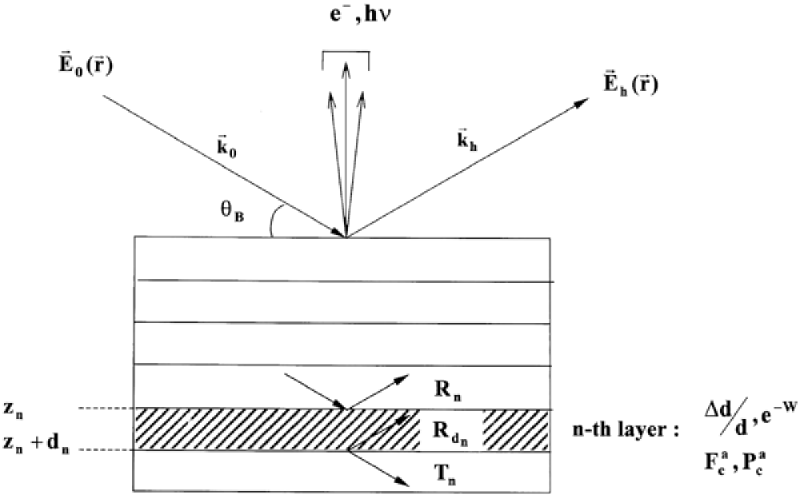
Figure 32: Schematic view of the SR yield from the multilayer crystal while the Bragg diffraction of x-rays. The n-th layer of such crystal is characterized by constant values of deformation $\Delta d/d$ and amorphization $e^{-W}$. The x-ray scattering from each layer is given by its reflection $R_{n}$ and transmission $T_{n}$ amplitudes. The SR yield from the n-th layer and the atoms of the sort $a$ is determined by the values of coherent fraction $F_{c}^{a}$ and coherent position $P_{c}^{a}$.

However, in many cases another approach [84] can be useful. One can divide deformed (and amorphisized) layer with an arbitrary shape on a several sublayers (see Fig. 32) with a constant structure parameters in each layer (these are in our case deformation $\Delta d/d$ and amorphization $e^{-W}$) and to solve TT equations in each sublayer analytically. Then substituting this solutions in the general equation (52) for the SR yield the desired result for a multilayer crystal can be obtained.

The details of this approach are given in the Appendix. Analytical solution of Eq. (24) for the amplitude $R(z,\theta)$ in the layer $z_{n}<z<z_{n}+d_{n}$ in the frame of the described model can be presented in the form of Eq. (114). In this equation both geometries of diffraction (Bragg and Laue) are considered simultaneously.

From the obtained solution it is easy to get standard recurrent equations. Defining by $R_{in}$ the reflection amplitude for both cases on the ”known” boundary ($R_{in}=R_{d_{n}}$ for Bragg case and $R_{in}=R_{n}$ for Laue), by $R_{out}$ the reflection amplitude on the unknown boundary and by $r_{out}$ solution for $R_{in}=0$ (reflection amplitude by thin layer) we have from (114-117)

$$r_{out}=\pm\frac{1-e^{\sigma d_{n}}}{x_{2}-x_{1}e^{\sigma d_{n}}}$$ (90)

$$R_{out}=\frac{r_{out}+TR_{in}}{1\mp r_{out}R_{in}},T=\frac{x_{2}e^{\sigma d_{n}}-x_{1}}{x_{2}-x_{1}e^{\sigma d_{n}}},$$ (91)

where $T$ is the transmission amplitude.

Directly from Eq. (32) solution for the direct beam $E_{0}(z,\theta)$ in the layer $z_{n}<z<z_{n}+d_{n}$ can be obtained in the form

$$E_{0}(z,\theta)=T(z,\theta)E_{0}(z_{0},\theta),$$ (92)

where $T(z,\theta)$ is the transmission amplitude through the layer defined in (121). Intensity transfer through the layer $I(\theta)=|E_{0}(d,\theta)|^{2}$ is determined by Eq. (122).

According to (52) the normalized SR yield from the n-th layer in general case of multiatomic unit cell for the sort of atoms $a$ and with the exponential form of the yield function (55) from the entrance surface can be presented in the following form

$$\kappa^{a}(\theta) = \chi_{i0}^{a}\int\limits_{z_{n}}^{z_{n}+d_{n}}dzP_{yi}(z)|T(z,\theta)|^{2}\times$$ (93)

$$\ \ \ \ \left\{1+\frac{|E_{h}(z,\theta)|^{2}}{|E_{0}(z,\theta)|^{2}}+2CRe\left[\frac{E_{h}(z,\theta)}{E_{0}(z,\theta)}\varepsilon_{\overline{h}}^{a}e^{i\varphi^{a}(z)-W^{a}}\right]\right\}.$$

Substituting to this expression previously defined functions we obtain

$$\kappa^{a}(\theta) = \chi_{i0}^{a}\int\limits_{0}^{d}dzP_{yi}(z)|T(z,\theta)|^{2}\times$$ (94)

$$\ \ \ \ \left\{1+\beta|Y|^{2}|R(z,\theta)|^{2}+2\sqrt{\beta}CF_{c}^{a}Re\left[YR(z,\theta)e^{i\varphi_{c}^{a}}\right]\right\}.$$

In this equation two important parameters of the theory i.e. coherent fraction ($F_{c}^{a}$) and coherent position ($P_{c}^{a}$) for the atoms of the sort $a$ in the n-th layer are introduced. They are defined as following

$$F_{c}^{a}=|\varepsilon_{\overline{h}}^{a}|e^{-W^{a}},\varphi_{c}^{a}=2\pi P_{c}^{a}=\Delta\varphi^{a}+\arg(\varepsilon_{\overline{h}}^{a})$$ (95)

and have a constant value in each layer, but can change from layer to layer.

Taking into account analytical solutions for the amplitudes $R(z,\theta)$ (114), $T(z,\theta)$ (121) and exponential form for the probability yield function $P_{yi}(z)$ (55) integral in expression for $\kappa^{a}(\theta)$ can be taken analytically (see Eq. (129) in Appendix). Finally the total yield of the SR from the whole multilayer crystal is the sum of the yields from every layer

$$\kappa_{tot}^{a}(\theta)=\sum\limits_{n=1}^{N}z_{n}(\theta)\kappa^{a}(\theta).$$ (96)

where $z_{1}=1$ and $z_{n}(\theta)=z_{n-1}(\theta)|T(d,\theta)|^{2}e^{-\mu_{yi}d}$. So, the whole algorithm for calculation of the angular dependence of the SR yield from the multilayer crystal in both (Bragg and Laue) geometries is formulated. In the following several examples of application of this approach will be given. We have to note here, that described in the previous Sections bicrystal model is a particular case of this more general approach with a number of layers $N=2$, where the second (thick) layer can be considered as a substrate and the top (thin layer) as an epilayer.

7.2 Applications

Described above approach of multilayer crystal was used in the papers [85, 86] where silicon crystals were implanted with $Fe$ and $Ni$ ions and analysed with XSW technique and Rutherford backscattering (RBS) method. The XSW technique was applied previously [8, 58, 87] for structure investigation of $Si$ crystals after implantation with the different impurity atoms ($As,$ $Bi$). However, in this papers more simplified model of the damaged crystal was assumed.

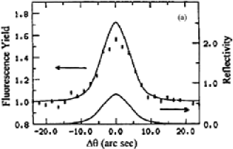
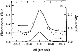
Figure 33: The fluorescence $FeK_{\alpha}$ yield for silicon crystals implanted with $Fe$ ions: just after implantation (a) and after annealing at $750^{\circ}$ (b). Points are experimental data and lines result of theoretical fitting (fitting parameters are summarized in Table 3). The reflectivity curve (c) for the sample ($Si$ (111) reflection, $CuK_{\alpha}$ radiation) is the same before and after annealing. From Ref. [86].

Below, following the papers [85, 86], we will discuss in details results of XSW analysis of silicon single crystals implanted with $Fe$ ions (dose $5\times 10^{15}$ ions/cm² at an energy of $80$ keV). After ion implantation samples were annealed at 750^∘ in the $N_{2}$ atmosphere. The fluorescence yield from $Fe$ atoms was measured. Results of this measurements on the samples before and after annealing are presented on Fig. 33.

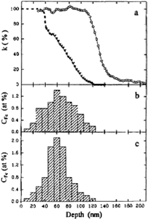
Figure 34: (a) Damage density in silicon due to $80$ $keV$ $Fe$ ion implantation for the sample just after implantation(circles) and after annealing (triangles). (b) Profile of $Fe$ impurity concentration for the sample just after implantation. (c) Profile of $Fe$ impurity concentration for the sample after annealing. From Ref. [86].

The RBS measurements were performed with 2 MeV ${}^{4}He$ ions. On Fig. 34 the results of the damage analysis from the RBS spectra are presented. On this figure the evolution of the $Fe$ atoms depth distribution is also shown. The measure of the damage density $k$ is given by the ratio of the displaced atom density to the crystal atom density , hence $k=100\%$ denotes a complete amorphization. An important feature of the $Fe-$atom depth distribution for an as implanted sample is its quasi-Gaussian shape with the maximum (i.e. $Fe$ mean projected range) located at the depth of 70 nm and range struggling of 80 nm. As it follows from the analysis the region of amorphization extends over 190 nm. After annealing the $Fe$ distribution become narrower, however, its maximum position did not change. Also the peak area has remained the same. This effect is apparently due to the low solubility of iron in silicon. In such a case the regrowth front pushes away impurity atoms in concentrations exceeding the solubility limit. Due to this process the impurity segregation occurs in a not yet regrown region.

For the theoretical fitting of the angular dependencies of the fluorescence yield for implanted region of the silicon sample a ”layered” model described in the first part of this Chapter was used. In the frame of this model each deformed layer was characterized by its constant value of thickness $d,$ deformation $\Delta d/d$ and amorphization factor $\exp(-W)$. Distribution of foreign atoms in these layers was characterized by two main parameters: $P_{c}^{Fe}-$ the coherent position, i.e. the position of the mean plane of the impurity atoms with respect to the diffraction planes of the crystal and $F_{c}^{Fe}$- coherent fraction, which describes the static and thermal displacements of the atoms from the mean position $P_{c}^{Fe}$ (see for definition Eq.(95)). Naturally, the contribution of each layer to the fluorescence yield is determined also by the concentration distribution $n_{c}^{Fe}$ of the impurity atoms in the surface layer of the silicon sample. All other parameters were the same in all layers.

For the theoretical fitting of the fluorescence yield from the implanted crystal before annealing 14-th layer model and after annealing 11-th layer model were used. The profile of amorphization $e^{-W}$ of the silicon surface and the distribution of implanted $Fe$ atoms $n_{c}^{Fe}$ for each layer were taken from the results of the RBS experiment (Fig. 34). The best fitting in the case of not annealed sample was obtained with the value of the coherent fraction $F_{c}^{Fe}=0.00\pm 0.02$. This result, as it was expected, mean that the implanted atoms occupy random positions in the lattice cell. Parameters of the layers and results of the fitting for the sample after annealing are summarized in Table 3. In addition to results obtained from RBS it was proposed that some parts of implanted atoms after annealing locate in substitutional positions of $Si$ atoms (parameter $P_{c}^{Fe}=0$). During the fitting procedure the coherent fraction of $Fe$ in the corresponding layers $F_{c}^{Fe}$ and the value of deformation $\Delta d/d$ of the surface layer were varied. To minimize the number of fitting parameters the uniform distribution of $F_{c}^{Fe}$ and $\Delta d/d$ in the surface layer for the depths $\simeq 40\div 120$ nm was taken. The best fitting result (see Fig. 33 and Table 3) gives for the average value of the surface relaxation $\Delta d/d=(-9.6\pm 0.09)\times 10^{-4}$ and the value of the coherent fraction $F_{c}^{Fe}=0.27\pm 0.02.$ This value of the coherent fraction means that approximately $27\%$ (with respect to the diffraction planes) of implanted $Fe$ atoms are in substitutional $Si$ positions. It is interesting to point here that from the independent XSW analysis it was obtained the same value of substitutional fraction of $Fe$ atoms as after the RBS analysis.

The obtained results show the effectiveness and mutual complementarity of the two methods for investigation of implanted crystals. The RBS experiments directly give the depth profiles of damage density for $Si$ surface layer and the profile of implanted ions concentration. The XSW analysis is the precise phase sensitive method. It gives directly the value of the phase $\varphi(z)$ that in our case is equal to $\varphi(z)=\mathbf{hu}(z)+\varphi_{c}^{Fe},$ where $\mathbf{u}(z)$ is the deformation of the surface layer (in the case of the uniform deformation we have $u_{z}=(\Delta d/d)L$ and $\varphi_{c}^{Fe}=2\pi P_{c}^{Fe}.$ As one can see from this expression the phase is the sum of deformation and the position of the impurity atoms in the unit cell and additional information is necessary to determine this two values independently. As it was shown in our analysis the combination of XSW and RBS methods gives us the opportunity to solve, in principle, this problem uniquely and determine positions of impurity atoms in the unit cell as well as the total deformation (relaxation) of the surface layer.

In the recent paper [88] for the analysis of the fluorescence yield from the superlattice crystal was also used a similar multilayer model.

8 Crystals with an extended deformation field

Up to now we were mainly considering the cases when the deformation field is located in the thin subsurface layer. However this condition is not always fulfilled. There exist a big class of deformations in crystals, that extends through the whole volume of the crystal. These are, for example, crystals with the Uniform Strain Gradient (USG), bent crystals, vibrating crystals and etc. In the following of this section we will show how x-ray standing wave analysis can be performed in such crystals.

8.1 Crystals with the uniform strain gradient. Bent crystals

Theory of x-ray standing wave behavior in crystals with USG and as a special case bent crystals was for the first time developed in papers [89, 90, 91]. Later similar theoretical approach for the analysis of the crystals with USG was performed in [92]. Investigation and characterization of crystals with USG (bent crystals) by different diffraction methods is of great practical interest - first of all, due to their wide application as x-ray monochromators at synchrotron radiation sources [93, 94] or focusing spectrometers for x-ray plasma diagnostics [95], and secondly, due to the fact that a lot of typical samples (e.g. implanted crystals, heterostructures) are often curved. Below we will present results obtained in [89, 90, 91].

The problem of the x-ray standing wave analysis in bent crystals is quite complicated due to the fact that the deformation field in such crystals is in general a two-dimensional function and extend through the whole volume of the crystal. Below we will consider a special case of such field: crystal with USG with the deformation field $\mathbf{hu}=Bz^{2}$, where $z$ is the depth from the crystal surface. If the incident wave is spherical and the source is on the Rowland sphere then cylindrically bent crystals are particular case of crystals with USG [28, 92].

The general problem of two variables in this specific case is reduced to determination of the amplitudes $\mathbf{E}_{0}(z)$ and $\mathbf{E}_{h}(z)$, which depend on one variable $z$. The x-ray amplitude $R(z,\theta)$ defined, as before, in the form (23) satisfies equation (24). In the case of the crystal with the USG an effective angular deviation parameter $y_{eff}(\theta,z)$ is a linear function from the depth $z$:

$$y_{eff}(\theta,z)=y(\theta)+y_{\varphi}(z)=y(\theta)+C(z/L_{ex}),$$ (97)

where $y(\theta),y_{\varphi}(z)$ are determined by the incident angle on the surface of the crystal (25) and the deformation field (26) and $C$ is the dimensionless parameter defining the strength of this field. For the cylindrically bent crystal the relationship between parameter $C$ and the curvature radius $R$ is given by [29]

$$C=-\frac{\lambda\gamma_{0}}{\pi X_{r}^{2}}\frac{1+\beta}{\beta R}\left[1-\beta\gamma_{h}^{2}(1+K)\right],$$ (98)

where $K$ is an elastic constant.

For the analysis of the angular dependence of the SR yield in the crystal with USG general equation (52) can be used. The type of the secondary process (fluorescence, photoemission) will be determined, as before, by the imaginary part of susceptibility $\chi_{0i}$ and probability yield function $P_{yi}^{a}(z)$.

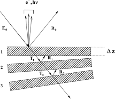
Figure 35: Schematic view of the multilayer model used for the calculation of the x-ray wavefield in a crystal with USG. Thickness of each layer is $\Delta z=L_{ex}/(mC)$. The angular deviation parameter $y_{i}(\theta)$ is constant in each layer and differs from layer to layer by the magnitude $\Delta y(\theta)=1/m$. The amplitudes $E_{0}$, $R_{n}$, $T_{n}$ are the amplitudes of incoming, reflected and transmitted beams from the n-th layer respectively.

Analytical solutions for the wave fields $\mathbf{E}_{0}(z)$ and $\mathbf{E}_{h}(z)$ in the crystal with USG were obtained in [96], however they can be effectively analysed only in their asymptotic form. The problem of x-ray Bragg diffraction and standing wave determination in a bent crystal can be effectively solved with numerical methods. In the papers [89, 90] the modified layer model described in the previous Section was used (see Fig. 35). The whole deformed crystal was divided into layers, each of thickness $\Delta z=L_{ex}/(mC)$, where $m$ is an integer. In each layer the value of the angular deviation parameter $y_{i}$ was considered constant and its value differs from layer to layer by the magnitude $\Delta y=1/m$ (parameter $m$ was taken from the condition of small change of $\Delta y$ from layer to layer). Analytical solution of Eq. (24) for $R(z,y_{i})$ in each such layer and, hence, in the whole crystal are given by (114). The angular dependence of the SR yield in the crystal with USG can be obtained straightforwardly by substituting the solutions for $R(z,y_{i})$ into Eq.(52), integrating it in each thin layer with the exponential probability yield function and summing over all layers (see Eqs. (94-96)).

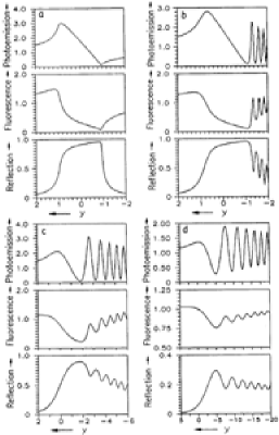
Figure 36: Angular dependences of the reflectivity, fluorescence and photoemission yield calculated for a cylindrically bent $Si$ (400) crystal, $CuK_{\alpha}$ radiation, at different values of the curvature parameter $C$: (a) $0$ (perfect crystal), (b) $0.1$, (c) $1.0$, (d) $10$. From Ref. [89].

The angular dependencies of the reflectivity and SR yield were calculated according to the described model for the different values of the parameter $C$. It was taken equal to $0$, $0.1$, $1$ and $10$, which, according to (98), correspond to the curvature radius $R$ equal to $\infty$, $550$ cm, $55$ cm and $5.5$ cm respectively. On Fig. 36 results of these calculations in the specific case of (400) symmetrical Bragg diffraction, $CuK_{\alpha}$, $\sigma-$polarized radiation in a thick $Si$ crystal are presented.

The behavior of the x-ray reflectivity (the broadening of the curves in the central part, oscillations on the tails of the curves) correspond completely to the behavior described for the first time in [29]. The angular dependencies of SR yield were calculated for the processes with the different depths of yield. Two cases were considered: fluorescence yield of $SiK_{\alpha}$ radiation (with $L_{yi}=70$ $\mu m$) and photoelectron yield (with $L_{yi}=0.1$ $\mu m$) from the atoms of the crystal matrix.

The behavior of SR at small values of parameter $C\leq 0.1$ (Fig. 36b) in the range of the angular parameter $|y|\leq 1$ differs only slightly from those for the perfect crystal (Fig. 36a). The photoemission yield ($L_{yi}<<L_{ex}$, $L_{ex}=3.6$ $\mu m$) for this angles has a dispersion like behavior and is quite sensitive to the phase shift. On the contrary, for the fluorescence yield ($L_{yi}<<L_{ex}$) due to extinction effect in the same angular region the characteristic dip is observed, which suppresses the phase sensitivity. However, already at small values of curvature characteristic oscillations can be seen on the tails of SR curves. They correspond to oscillations on x-ray reflectivity curve. With increasing curvature one can see first of all a broadening of the phase-sensitive region and secondly the increasing of the amplitude of the oscillations on the tails of the photoemission yield curves (Fig. 36c). For large values of curvature the SR yield curves become, on the average, flatter and flatter and the period of oscillations is increased (Fig. 36d). These curves correspond to a strongly deformed crystal. So, in the case of the curved crystal we have an interesting possibility to study on the same sample the standing wave behavior in both limits of a weakly and strongly deformed crystal.

The x-ray standing wave field behavior in the bulk of the deformed crystal is determined first of all by the type of deformation in the crystal (see for e.g. [50, 71]). Reflectivity $P_{R}(z,y)$ and x-ray standing wavefield in the bulk of the crystal with USG were analysed in details [90]. The intensity of the wavefield on the depth $z$ has the form

$$I(z,y)=\left|E_{0}(z,y)\right|^{2}\left|1+\sqrt{\beta}YR(z,y)e^{i\Delta\varphi_{c}^{a}}\right|^{2}$$ (99)

and the phase shift $\Delta\varphi_{c}^{a}$ is determined by the positions of the impurity atoms relative to diffraction planes. The values of $E_{0}(z,\theta)$ and $R(z,\theta)$ were calculated according to the model described before.

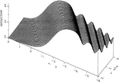
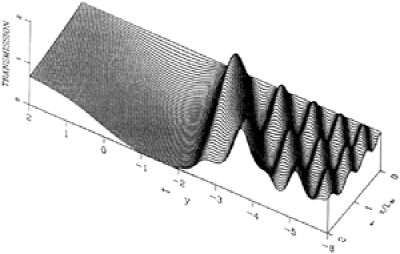
Figure 37: The two-dimensional distribution of the reflectivity $P_{R}(z,y)$ (Top) and transmitted wave intensity $T^{2}=|E_{0}(z,y)|^{2}$ (Bottom) calculated at the depths $z=0\div 2L_{ex}$ for the curvature parameter $C=1$. From Ref. [90].

On Fig. 37a two-dimensional distribution of the reflectivity $P_{R}(z,y)$ in the ($z,y$) plane is presented. Calculations were made for the parameter $C=1$ and for the depths $z=0\div 2L_{ex}$. As it follows from the obtained result for a crystal with USG the reflectivity at an arbitrary depth $z$ (while remaining invariable in its shape) is shifted in the angular range according to (97). Such behavior of the reflectivity indicates that at the depth $z$ there exist an angular region of the total reflection of x-rays where the phase of the field amplitude changes from $0$ to $\pi$ (so-called phase-sensitive region). For the fixed incident parameter $y_{0}(\theta)$ that region is located at the depth $z_{eff}\sim\left|y_{0}(\theta)L_{ex}/C\right|$ and has an effective thickness $\Delta z_{eff}\sim\left|2L_{ex}/C\right|$. Thus the size of this region is determined by the value of the parameter $C$.

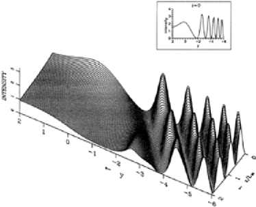
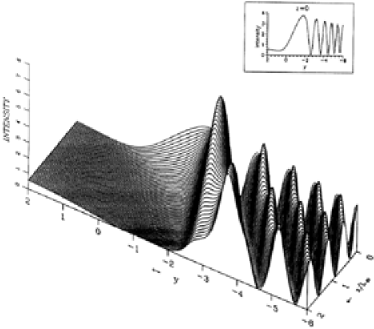
Figure 38: The two-dimensional distribution of the standing wave intensity $I(z,y)$ calculated at depths $z=0\div 2L_{ex}$ for the curvature parameter $C=1$. In the inset the angular dependence of the intensity for $z=0$ is plotted. (Top) Intensity values calculated on diffraction planes ($\Delta\varphi_{c}^{a}=0$). (Bottom) Intensity values calculated between diffraction planes ($\Delta\varphi_{c}^{a}=\pi$). From Ref. [90].

The two-dimensional distribution of the intensity $I(z,y)$ (99) in the ($z,y$) plane for the same value of the parameter $C$ are shown on Fig. 38. On Fig. 38a intensity of the wavefield is calculated on the diffraction planes ($\Delta\varphi_{c}^{a}=0$) and on Fig. 38b between the diffraction planes ($\Delta\varphi_{c}^{a}=\pi$). Comparing these intensity distributions one can notice that they differ both by the value and by the position of oscillations the tails of the curves. This effect of phase sensitivity of the standing wave intensity (99) in the bulk of deformed crystal (contrary to the case of perfect crystal) can be understood if the behavior of the transmitted wave intensity $T^{2}(z,y)=\left|E_{0}(z,y)\right|^{2}$ in the crystal with USG is analysed.

The two-dimensional distribution of the transmitted wave intensity $T^{2}(z,y)$ in the ($z,y$) plane for the parameter $C=1$ is presented on Fig. 37b. According to the analysis performed in Section 4 the phase sensitivity of the standing wave intensity in the bulk of the perfect crystal at depths $z\simeq L_{ex}$ is suppressed by the extinction effect. The situation is quite different in the case of the crystals with USG (see Fig. 38b). This more complicated picture is a result of interference of the incident and diffracted waves with a deformation field of a crystal. This interference gives rise to an increase of the transmitted wave on the edge of the phase-sensitive region even at the depths $z\simeq L_{ex}$ (Fig. 37b). Just due to this effect the phase sensitivity of the standing wave intensity in the bulk of the crystal with USG is increased (Fig. 38). Therefore, although for the perfect crystals applications of the standing wave method are limited to thin subsurface layers in the case of the crystals with USG this method can be extended to investigation of thin buried layers (monolayers) of impurity atoms even located at the depths $z\geq L_{ex}$.

Different calculation approach was used in the paper [91] (see also ([92])) for the analysis of x-ray standing wave field on the surface of the crystals with USG (deformation field was taken in the same form $\mathbf{hu}(\mathbf{r})=B\cdot z^{2}$, where $B$ is a constant). According to this approach the amplitudes of the x-ray field $\mathbf{E}_{0}(\mathbf{r})$ and $\mathbf{E}_{h}(\mathbf{r})$ were obtained from the direct integration of the TT equations in the form (13). For the details of this calculation algorithm in the Bragg geometry of diffraction see, for example, review paper [97].

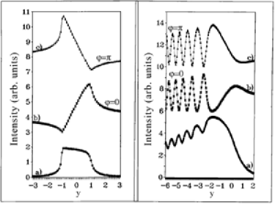
Figure 39: The angular dependence of the x-ray reflectivity (a) and the x-ray standing waves (b and c) calculated on the surface of the $Si$ (400) crystal without deformation (left figure) and with a USG (right figure). The XSW curves correspond to different position (the phase shift $\Delta\varphi_{c}^{a}$) of the impurity atoms on the surface of a crystal. From Ref. [91].

In the paper [91] the angular dependencies of x-ray reflectivity and intensity of x-ray standing waves (99) on the surface of the crystal with USG were calculated for the case of (400) symmetrical Bragg diffraction, $CuK_{\alpha}$, $\sigma-$polarized radiation in a thick crystal of silicon. Results of these calculations are presented on Fig. 39. The XSW curves on the surface of the crystal were calculated as before for two different values of the phase $\Delta\varphi_{c}^{a}=0$ and $\Delta\varphi_{c}^{a}=\pi$ that correspond to coordinate $\mathbf{r}$ on the surface of the bent crystal, that either coincide with the position of the diffraction planes or to the position between diffraction planes. In the calculations the USG constant $B$ was taken equal to $B=2\cos^{2}\theta_{B}(1/L_{ex}^{L})\beta_{c}$, where $\beta_{c}=\pi/(2L_{ex}^{L})$ is the critical value used in the theory of x-ray propagation in bent crystals [97] and $L_{ex}^{L}$ is the extinction length in the symmetric Laue case. This value of constant $B$ correspond to parameter $C=1$ from Eq. (98). The XSW curves in the deformed crystal comparing to that in the perfect one (Fig. 39) shows broadening in the central part (in the so-called phase sensitive region) and also a sharp oscillations on the tails that correspond to oscillations on the reflectivity curve. The angular position of these oscillations depend first of all on the strength of the deformation field (determined now by the value of parameter $B$) and also on the phase shift value $\Delta\varphi_{c}^{a}$. The origin of this oscillation is the waveguide character of X-ray propagation in crystals with USG [29]. It is important to note here, that the standing wave picture obtained from the direct numerical calculations of the TT equations for the crystals with the USG are in a good agreement with the simplified multilayer model used in [89, 90] and described in the beginning of this Chapter. However, from the point of the waste of the computer time the first method is much more effective.

8.2 Vibrating crystals

Another case of x-ray standing waves in the crystals with extended deformation field: namely vibrating crystals was considered in the paper [98]. If in the previous subsection the deformation field in crystal can be controlled by the strain gradient or radius of curvature in the case of vibrating crystal this can be achieved by changing the amplitude and the wave vector of ultrasonic excitations in the crystal. What is more important for x-ray standing wave technique - extinction length in vibrating crystals can be also tuned in controllable way. The periodic deviation of the reflection planes from their ideal position in a perfect crystal misorientates the inner crystalline structure of the crystal, effectively ”switching off” the whole parts of the crystal from the dynamical diffraction scattering. Increasing of the ultrasonic amplitude increases the deformation field and due to its periodic structure creates new dynamical reflexes (satellites) with extremely big effective extinction length. In a limit of a big ultrasonic amplitude, one can achieve the kinematical limit of diffraction when the initial reflecting power of the crystal is distributed over the large angular interval.

Below, following [98], the angular dependence of the SR yield will be considered for the special case of vibrating crystals, crystals disturbed by longitudinal ultrasonic vibrations propagating normally to the crystal surface. The advantage of this scheme is the uniform distribution of the deformation field along the crystal surface ant its layered structure in the bulk of the crystal.

In this case a vibrating crystal can be presented by a set of identical layers with thickness equal to the period of the ultrasonic wave. Every layer can be approximated by a combination of thinner layers with constant value of interplaner distance (see Fig. 40). This periodic structure give rise to an additional satellites in the reciprocal space with the position $\mathbf{h}+n\mathbf{K}_{s}$, where $\mathbf{K}_{s}$ is the wave vector of the ultrasonic wave. With increasing the amplitude of the ultrasonic wave the undisturbed part of the crystal (and the reflecting power of the main reflex) decreases whereas the fraction corresponding to the satellites increases. Below the special case of the so-called ”high-frequency” ultrasonic wave, when the ultrasonic wavelength is smaller then the extinction length of the given reflection will be considered. This gives the possibility of investigating each satellite independently, because they do not overlap in the angular range with each other and with the main reflex.

The displacement field of the ultrasonic standing wave will be taken in the following form

$$\mathbf{u}(z,t)=\mathbf{w}\cos\omega t\cos K_{s}z,$$ (100)

where $\mathbf{w}$ and $\omega$ are the amplitude and frequency of the ultrasonic vibrations (the wave vector $\mathbf{K}_{s}$ is directed along the normal to the crystal surface).

The dynamical symmetrical x-ray diffraction on a thick crystal with the diffraction vector $\mathbf{h}$ directed along the normal to the crystal surface (axis $z$) will be considered below. The x-ray wavefield amplitudes $E_{0}(z,\theta)$ and $E_{h}(z,\theta)$ in the displacement field (100) can be effectively found from the set of TT equations (18). In this case Fourier component of the susceptibility of the deformed crystal $\chi_{h}^{d}$ can be presented as an infinite sum

$$\chi_{h}^{d}=\chi_{h}e^{i\mathbf{hu(}z\mathbf{)}}=\chi_{h}\sum_{n=-\infty}^{\infty}J_{n}(\mathbf{hw})i^{n}\exp(inK_{s}z),$$ (101)

where $J_{n}(\mathbf{hw})$ is the Bessel function of real argument. Each term in the infinite sum (101) correspond to the satellite with the diffraction vector $\mathbf{h}+n\mathbf{K}_{s}$. At small values of the ultrasonic amplitude $\mathbf{w}$ only two first order satellites ($n=\pm 1$) are essential in the expansion (101). The amplitudes $E_{0}(z,\theta)$ and $E_{h}(z,\theta)$ can be also expanded in the same way

$$E_{g}(z,\theta)=\sum_{n=-\infty}^{\infty}E_{g,n}(z,\theta)\exp(inK_{s}z),g=0,h.$$ (102)

Substituting expression (102) into TT equations (18) it is possible to obtain a set of similar equations for the amplitudes $E_{0,n}(z,\theta)$ and $E_{h,n}(z,\theta)$ with the following substitution $\chi_{h}\rightarrow\chi_{h,n}$ and $\alpha\rightarrow\alpha_{n}$, where

$$\alpha_{n}=\alpha+nK_{s}\frac{\lambda\gamma_{h}}{\pi}\mbox{ and }\chi_{h,n}=i^{n}J_{n}(\mathbf{hw})\chi_{h}$$ (103)

are the new values of angular deviation parameter and susceptibility of the n-th satellite. After straightforward calculations analytical solutions for the amplitudes of transmitted (only component $E_{0,0}(z,\theta)$ is important) and diffracted $E_{h,n}(z,\theta)$ wave in the vicinity of the n-th satellite can be obtained (see for details [98]).

The x-ray wavefield in the vicinity of the n-th satellite has the form of a standing wave with the period $2\pi/|\mathbf{h}+n\mathbf{K}_{s}|$

$$E\simeq E_{0,0}e^{i\mathbf{k}_{0}\mathbf{r}}+E_{h,n}e^{i(\mathbf{k}_{h}+n\mathbf{K}_{s})\mathbf{r}},$$ (104)

It is important to note here that the period of the standing wave does not depend effectively on the order of the satellite, because the diffraction vector is much bigger than the wave vector of ultrasonic wave. The only parameter varying from satellite to satellite is the effective extinction length. In the angular region of the n-th satellite the effective extinction length is equal to

$$L_{ex}^{n}=\frac{L_{ex}}{|J_{n}(\mathbf{hw})|},$$ (105)

where $L_{ex}$ is the extinction length in the undisturbed crystal. According to (105) an effective extinction length is a function of the ultrasonic amplitude $\mathbf{w}$ and can be tuned by the change of the voltage applied to ultrasonic transducer.

The secondary radiation yield from the vibrating crystal can be obtained in the frame of the general theory discussed in Chapter 3. Substituting the obtained values of the wave fields $E_{0,0}(z,\theta)$ and $E_{h,n}(z,\theta)$ into Eqs. (49, 50) the angular dependence of the total secondary radiation yield $N_{n}(\theta)$ in vibrating crystal on the n-th satellite can be presented in the form of the infinite sum

$$N_{n}(\theta)=\sum_{m=-\infty}^{\infty}N_{n,m}(\theta).$$ (106)

Each term in this expansion can be calculated analytically if exponential form (55) for the probability yield function $P_{yi}(z)$ is assumed. Finally it was obtained [98] that every term $N_{n,m}(\theta)$ in expansion 106 is proportional to the relative contribution of the scattering potential $J_{m}(\mathbf{hw})$ and through this Bessel function depend on the value of the amplitude of the ultrasonic wave.

This theoretical approach was applied for the calculation of the photoelectron yield (with the depth of yield $L_{yi}=0.2\mu m$) from $Si$ (111) crystal $CuK_{\alpha}$ radiation. The ultrasonic wavelength $\lambda_{s}$ was taken equal to $0.7\mu m$. In this case general equations can be simplified and in the limit of small ultrasonic amplitude the photoelectron yield near two first satellites ($n=\pm 1$) is equal to (higher order terms in expansion (106) can be neglected)

$$N_{1}(\theta)\simeq N_{1,1}(\theta)+N_{1,0}(\theta)+N_{1,-1}(\theta).$$ (107)

At the same time contributions to the main reflex from two first-order satellites are completely compensated and the total SR yield can be approximated by the expression

$$N_{0}(\theta)\simeq N_{0,0}(\theta).$$ (108)

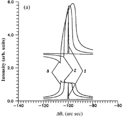
Figure 41: The angular dependence of the photoelectron yield and reflectivity calculated for the values of the amplitude $\mathbf{hw}$ equal to $0.1$ (curve 1), $0.5$ (curve 2), $0.9$ (curve 3). Figures (a) and (c) correspond to satellites with $N=\mp 1$ and (b) to the main reflex ($N=0$).From Ref. [98].

Results of numerical calculations of the angular dependence of the photoelectron yield for the different values of ultrasonic amplitude $\mathbf{hw}=0.1,0.5,0.9$ are presented on Fig. 41. As it follows from the numerical calculations the photoelectron yield near the main reflex varies very slowly, however, the yield excited in the angular range of the satellites is very sensitive to the value of the ultrasound amplitude.

It is important to note here that approach discussed in this subsection gives the intensity of the diffracted x-ray waves and the intensity of the SR yield for a fix time. In ordinary x-ray scattering experiment on vibrating crystals only the quantities averaged over the period of vibrations are measured. However results discussed here can be, in principle, observed in stroboscopic experiments, that are available on synchrotron radiation sources. The coincidence between the time-periodic flashes of the synchrotron radiation beam and the period of the ultrasonic vibrations gives the possibility to scatter the x-ray wave on the ”frozen” distorted lattice.

In the recent paper [99] developed above theory was extended for the case of the yield of the thermal diffuse scattering in vibrating crystals.

9 Phase problem

It is well known, that in any experiment based on the scattering of radiation by condensed matter, the measured quantity is an intensity, from which one can determine only the modulus of the complex valued scattering amplitude. In order to obtain comprehensive information about the structure of the scattering object, however, it is also necessary to know the phase of this amplitude. This is a general problem of scattering that arises in many applications, for example, in the study of the structure of the surface layers of single crystals by means of x-ray scattering. In this case the structure of the surface layer is directly connected via Fourier transform with the angular dependence of the scattering amplitude. At the same time a standard x-ray diffraction experiment does not give an opportunity to determine the phase of this amplitude.

To solve this problem of phase determination indirect methods are widely used in x-ray crystallography (see for review of different methods a book [100]). During last years it was a rapid development of the direct methods for the phase determination of the structure factors, for example, by means of multibeam diffraction [38, 39, 40, 101]. Another direct method of the structure analysis and phase determination is based on XSW method. As it was demonstrated in Chapter 4 coherent fraction $F_{c}^{a}(\mathbf{h})$ and coherent position $P_{c}^{a}(\mathbf{h})$ represent, in fact, the $\mathbf{h}-$th amplitude and phase of the Fourier decomposition of the distribution of atoms under consideration (see also [58, 61]). Due to availability of the synchrotron radiation sources of the third generation new methods based on the utilization of the high coherency properties of the synchrotron radiation for the phase determination has become possible [102, 103]. In this case powerful iterative methods for the phase retrieval are used [104].

Here we will discuss another approach for the direct phase determination of the scattering amplitude based on the simultaneous measurements of the reflectivity and SR yield in the large angular range. This information can be used for the direct and what is very important unique determination of the profile of the structural changes of the crystal surface layer. The idea of this method was for the first time proposed in [32] and later realized practically in [105].

If the thickness $L_{d}$ of the deformed layer in the sample satisfies the condition $L_{d}<<L_{ex}$, where $L_{ex}$ is the extinction length, then the scattering of x-rays by this layer is kinematic and the scattering amplitude $R(\theta)$ is given by

$$R(\theta)=\left|R(\theta)\right|e^{i\alpha(\theta)}=R_{0}\int\limits_{0}^{\infty}dzF(z)e^{iq(\theta)z},F(z)=f(z)e^{i\varphi(z)}.$$ (109)

Here $R_{0}=-i\pi\chi_{h}/(\lambda\sin\theta_{B})$, $q(\theta)=(4\pi/\lambda)\cos\theta_{B}\Delta\theta$, $f(z)=\exp(-W(z))$ is the static Debye-Waller factor and $\varphi(z)=\mathbf{hu}(z)$. According to expression (109), outside the region of the total reflection the scattering amplitude $R(\theta)$ is the Fourier transform of the complex function $F(z)$. This function and thus the structure of the surface layer can be reconstructed directly by the use of the inverse Fourier transform. However, it is necessary to know both the amplitude and phase of $R(\theta)$.

The amplitude of $R(\theta)$ can be obtained from the angular dependence of the reflectivity curve measured in a big angular range far from the exact Bragg condition according to equation

$$P_{R}(\theta)=C_{p}\left|R\left(\theta\right)\right|^{2},$$ (110)

where $C_{p}$ is a polarization factor equal to $C_{p}=(1+C^{3})/(1+C)$ in a double-crystal experimental scheme and parameter $C$ is defined in (20).

The phase $\alpha(\theta)$ of the scattering amplitude $R(\theta)$ can be determined by measuring SR yield with a small depth of yield $L_{yi}$ satisfying the condition: $L_{yi}<<L_{d}$ in a big angular range far from exact Bragg condition. This can be, for example, photoelectron yield coming from the submicron depths of the sample or the fluorescence yield of the foreign atoms absorbed or implanted on the top of the sample. This angular dependence can be obtained directly from the general equation (52) and is equal to

$$\kappa(\Delta\theta)=1+C_{p}\left|R(\Delta\theta)\right|^{2}+2C_{p}\left|R\left(\Delta\theta\right)\right|\left|\varepsilon_{\overline{h}}\right|f(0)\cos\left[\Phi_{R}(\Delta\theta)+\varphi(0)+\arg(\varepsilon_{\overline{h}})\right],$$ (111)

where $f(0)$ and $\varphi(0)$ are the values of the static Debye-Waller factor $f(z)$ and phase $\varphi(z)$ at $z=0$. As it follows from (110) and (111) by simultaneous measurement of the reflectivity $P_{R}(\theta)$ and SR yield $\kappa(\theta)$ both the amplitude $\left|R\left(\Delta\theta\right)\right|$ and the phase $\alpha(\theta)$ of the scattering amplitude $R(\theta)$ is obtained uniquely in the whole angular range. The values of $f(0)$ and $\varphi(0)$ can be found from the fitting of the central part of curves $P_{R}(\theta)$ and $\kappa(\theta)$, where conditions of the strong dynamical scattering are satisfied. Finally, using inverse Fourier transform, the structure of the damaged layer can be obtained directly.

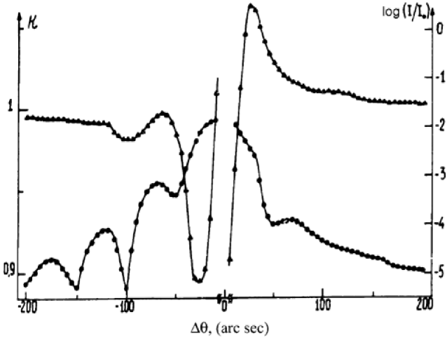
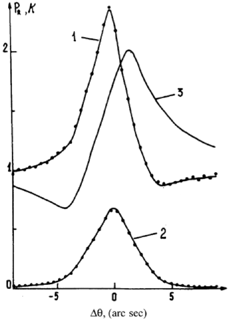
Figure 42: Photoemission yield (upper curves) and x-ray reflectivity (bottom curves) measured at big deviations from exact Bragg condition (Top) and in the region of the strong Bragg diffraction (Bottom). Points are experimental data and lines are theoretical calculations. Curve 3 on Bottom Figure correspond to the photoemission yield from an ideal silicon crystal. From Ref. [105].

In the paper [105] this approach was applied for the determination of the depth profile of distortions of the surface layers of silicon crystals after implantation. Samples were implanted by $B^{+}$ ions (with energy of 100 keV, dose of $10^{15}$ $cm^{-2}$) and then annealed ($T=800^{\circ}C$, $t=10$ $\min$) in an oxidized atmosphere. In experiment the (400) reflection and $CuK_{\alpha}$ radiation were used. The photoelectron emission and the x-ray reflectivity from the samples were measured both at large deviations from the Bragg angle (Fig. 42a) and in the region of total reflection (Fig. 42b). Electrons from $K-$shell with energies from $5.9$ keV to $6.4$ keV were excited and detected by a gas proportional counter with a resolution $\approx 15\div 20\%$. According to Eq. (56) an estimated depth of yield of this electrons was equal to $L_{yi}=0.1$ $\mu m$.

It is important to note here, that reflectivity curves obtained in a standard double-crystal scheme of measurements are the superposition of coherent and incoherent scattering channels and therefore are inapplicable for our theoretical analysis, where only coherent part of the scattered radiation has to be used for the phase retrieval. This problem can be solved by measuring the ”tails” of the reflectivity curves in a triple-crystal scheme. This arrangement makes it possible to separate the coherent part of scattering from its incoherent part [106].

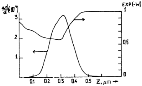
Figure 43: Profiles of the deformation $\Delta d/d(z)$ and of the static Debye-Waller factor $f(z)=\exp(-W)$ obtained as a result of the phase retrieval from the angular dependence of the photoemission yield and reflectivity (Fig. 42a). From Ref. [105].

Photoemission curve in the region of the strong dynamical diffraction (Fig. 42b) is similar to the inverted curve from an ideal crystal. It coincides with theoretical one with the values of the phase $\varphi(0)=2.3$ and static Debye-Waller factor $f(0)=0.9$. Described above algorithm for the phase reconstruction was applied to obtain the structural information about the surface layer of the sample from the ”tails” of experimentally measured curves (Fig. 42a). Profiles of the deformation $\Delta d(z)/d$ and Debye-Waller factor $f(z)$ obtained according to this approach are presented on Fig. 43. From this Figure it is well seen, that the deformation in the damaged layer is positive and reaches its maximum at a depth $L\approx 0.3$ $\mu m$. This result correlates well both with the distribution of $B^{+}$ ions in silicon lattice under the conditions of implantation and the theory for defect formation in these crystals [107]. We have to note here, that all calculations were carried out in the limit $L_{yi}\rightarrow 0$. The final depth of yield of the photoelectrons can be also taken into account, however, this does not change result essentially.

Finally, in the paper [105] it was presented a method for a direct solution of the phase problem while the x-ray scattering in the deformed crystal. From simultaneous measurements of the photoelectron emission and reflectivity curves in a big angular range near exact Bragg angle the complex scattering amplitude can be determined completely and thereby the structure of the deformed surface layer can be reconstructed uniquely.

10 Conclusions

Traditionally, since the discovery of x-rays, x-ray diffraction methods were used to obtain structural information from different type of crystals, including protein crystals [100]. In this review we have shown how during last 20 years combination of the traditional x-ray diffraction and x-ray standing wave technique has become one of the most sensitive methods of studying structure of real crystals. Here we have treated in detail the problems involved in theoretical studying and practical application of x-ray standing wave method for the structural analysis of the surface layers. Starting from the perfect crystal, crystals with amorphous surface layer were analysed. Then theory and different applications of the simplest model of deformed surface layer, so-called bicrystal model were presented. This model was generalized for the case of a multilayer model. Analytical approach for the secondary radiation yield from such crystal was analysed in details and different applications of this approach were discussed. It was shown, that both geometries of diffraction Bragg and Laue can be studied in the frame of one theoretical approach. However x-ray standing waves and secondary radiation yield in Laue geometry has its own peculiarities different from Bragg geometry and they were discussed separately. This theory was generalized for the case of the crystals with an extended deformation field, such as crystals with a uniform strain gradient (bent crystals) and vibrating crystals. We have also discussed the possibilities of the direct measurements of the phase of the scattering amplitude from deformed crystal and presented the way of the unique reconstruction of the structure of this deformed layer.

During last decade new materials with high crystal quality has appeared such as High-T_c superconductors, quasicrystals, isotopically pure materials. This opens the possibility to use XSW analysis in such crystals. For example, High-T_c superconducting crystals $Nd_{1.85}Ce_{0.15}CuO_{4-\delta}$ and ultrathin films of YBa₂Cu₃O₇ on SrTiO₃(001) were studied with XSW method in [64, 108]. Fluorescence radiation from $AlPdMn$ icosahedral quasicrystal excited by standing waves formed from x-ray reflections along a twofold symmetry axis was measured in a recent paper [109], lattice constants of the isotopically pure layers of ${}^{76}Ge$ grown on natural germanium were determined while the photoelectron yield XSW studies in [78]. The effect of different methods of growth on the interface quality of extremely thin buried $Ge$ $\delta$ layers in $Si$ were studied by means of different diffraction techniques including XSW [110]. Photoelectron yield and fluorescence radiation from $(AlAs)(GaAs)$ short-period superlattices was measured in [88, 111, 112].

One interesting approach in XSW analysis was developed in [113]. Kossel diffraction in perfect crystals can be viewed as the reverse process of x-ray standing waves with the source of radiation located inside the crystal. New experimental method was proposed in this paper for determination of atomic positions in the bulk or at a surface of a crystal by analysing the profile of angularly resolved Kossel lines.

In the last years different theoretical approaches were elaborated for the analysis of XSW in real crystals. For example, x-ray standing waves in crystals with statistically distributed defects were analysed theoretically in [114, 115]. Analytical results for standing wave behavior in the deformed crystal with a special type of deformation were obtained in [24]. Standing waves in Laue geometry for a special type of scattering with only imaginary part of the atomic scattering factor were analysed theoretically in [116].

As it was shown in our review in many situations it is important to reduce the signal coming from the background and to enhance the surface contribution. From this point it is quite favorable to make experiments in grazing incidence geometry proposed for the first time by W.C. Marra, P. Eisenberger and A.Y. Cho [117] and later developed as a useful tool for surface sensitive XSW measurements in a number of papers [118, 119, 120, 121] (see also a book [12]).

In this review paper we were discussing in details formation of XSW field in the case of two-beam dynamical diffraction in real crystals. This approach can be generalized for the case of multibeam dynamical diffraction. This was done for the first time theoretically in [68, 122]. Angular dependencies of the photoelectron yield in the multibeam region for the case of four-beam ($220/400/\overline{2}20$) and three-beam ($444/335$) dynamical diffraction in $Si$ perfect crystals were calculated. If in the case of two-beam diffraction in one measurement information about atomic distribution in the sublattice can be obtained only along $\mathbf{h}$-vector, in the case of the multibeam diffraction when second reciprocal vector $\mathbf{g}$ is involved in diffraction process one can obtain structural information simultaneously in both directions. For the first time fluorescence measurement in the case of multibeam diffraction for a perfect crystal was performed in [123], later photoemission yield from a perfect $Si$ crystal for the case of ($111/220$) three-beam diffraction was measured in [124, 125] (see also for review of this results [126]). Here we would like to mention also another method of direct measurement of the phase of the structure factor or total deformation field in thin surface layers without measuring any SR yield. This method is based on the measurement of the ”weak” three-beam reflection far from the multibeam region simultaneously with the strong one. In this case intensity of this reflection can be presented in the form

$$I_{g}\sim\frac{1}{\alpha_{g}^{2}}\left|E_{0}+e^{i\mathbf{hu}(0)}\frac{\chi_{gh}}{\chi_{g0}}E_{h}\right|^{2},$$ (112)

where $\alpha_{g}$ is the angular deviation from exact multibeam Bragg region. This expression is similar to (77) obtained for the SR yield with the small depth of yield. This approach was for the first time applied for the measurement of the phase of the structure factor in perfect crystals in [101] and then generalized for the case of deformed crystals theoretically [122, 127] and experimentally [128].

Approach described in this review paper to the calculation and analysis of the secondary radiation yield while the dynamical diffraction of x-rays was quite general. However we have restricted ourself mainly with the cases of fluorescence and photoelectron yield. Actually the potentialities of applications of x-ray standing waves are much broader. They include for example the study of such inelastic processes as thermal diffuse and Compton scattering and internal photoeffect under conditions of dynamical diffraction of the incident radiation. Every process has its own peculiarities and contains information of a fundamentally new type.

For example, a unique information about high–order total photoelectron cross sections, radial wave functions and electron wave phase shifts can be obtained from XSW angular resolved and integrated photoelectron yield (see for theoretical and first experimental results [48, 49, 129, 130, 131]). We want to mention here also recent results [132] where the photoelectron yield in the field of XSW was measured from the valence band of the Ge and GaAs crystals giving the possibility to measure the bond polarity parameter.

Thermal diffuse and Compton scattering in the conditions of dynamical diffraction were studied experimentally starting from the 60-th [13, 14, 15] (see also theoretical work [44]). In [16] it was shown the possibility to determine the values of the phonon eigenvectors directly from XSW experiment. In the theoretical papers [45, 46] unified Green function approach to the problem of the yield of the thermal diffuse scattering was elaborated and it was shown that surface contribution in a special diffraction conditions can become important. Compton scattering in the XSW field was studied intensively in 80-th [133, 134, 135, 136, 137, 138, 139, 140] (see also for review of this results [141]). In this papers it was shown, that investigation of the coherent Compton scattering opens the possibility for determination of non-diagonal elements of the density matrix [136] and contribution of the valence electrons to the atomic factor of the x-ray scattering [138, 139, 140].

Measurements of the photoelectric current in a semiconductor crystals while the dynamical scattering of x-rays [17, 18] opens the possibility to study both the structural and the electrophysical characteristics of the crystal simultaneously. In a series of papers [142, 143] it was demonstrated, that the depth of yield in this case is determined by the diffusion length $L_{d}$ of minority carriers. X-ray luminescence studies of phosphor crystals excited by x-ray standing waves were carried out in [144].

In this review paper we were mainly discussing the possibilities of generating the XSW in real crystals not in extreme conditions. However, there are exist some ways for generating x-ray standing waves in so-called extreme conditions with Bragg diffraction close to $\theta_{B}=90^{\circ}$ and total external reflection (so-called $0-$th order Bragg reflection). Due to extreme broadening of the Darwin curve in the first case (the half-width of the curve $\Delta\theta_{1/2}$ in this case is proportional to$\sqrt{\chi_{h}}$) this conditions of generating XSW can be effectively applied for less perfect for e.g. mosaic crystals (see for modifications of the dynamical theory [145, 146] and for XSW measurements [147, 148, 149, 150] and also review paper [23]).

The case of the total external reflection can be treated as a special case of dynamical diffraction with $0-$th order Bragg reflection. The amplitude ratio for the reflected amplitude $E_{R}$ to the incident amplitude $E_{0}$ can be obtained from the Fresnel formula [151] or directly from (23, 31) with $\theta_{B}=0$, $\chi_{h}=\chi_{0}$ and approximation $\sin\theta\approx\theta$

$$\frac{E_{R}}{E_{0}}=\frac{\theta-\sqrt{\theta^{2}+\chi_{0}}}{\theta+\sqrt{\theta^{2}+\chi_{0}}}.$$ (113)

The peculiarity of XSW at the total external reflection is the strong variation of the wavefield spacing from the reflection angle from about 50 Å for $\theta\approx\theta_{c}$ (where $\theta_{c}=\sqrt{|\chi_{0}|}$ is the critical angle) to infinity for $\theta\rightarrow 0$. For experimental and theoretical results of XSW measurements in the total reflection conditions see for e. g. [152, 153, 154, 155, 156].

Another way to generate an x-ray interference field with long-period wavefield spacing is the use of Bragg diffraction from Layered Synthetic Microstructures (LSM) or organic Langmur-Blodgett (LB) multilayers. Naturally, for generating standing waves these structures has to be periodic. Alternating amorphous layers of high$-Z$ low$-Z$ materials (e.g. $W/C,$ $Rh/C$ or $Ni/C$ and etc.) provides high maximum reflectivity. The lattice plane spacing in such materials can typically range from 15 to 200 Å. After the first demonstration by Barbee and Warburton [157] of the possibility to use these structures in XSW analysis it was applied effectively in a number of papers [158, 159, 160, 161, 162, 163].

In conclusion we can see that XSW method due to its unique properties of combination of the x-ray dynamical diffraction with spectroscopic technique has become a powerful tool in modern crystallography and even more general in condensed matter physics.

11 Appendix

Secondary radiation yield from a multilayer crystal

(analytical approach)

In Appendix we will give the details of the analytical approach (following [84]) for the angular dependence of the SR yield for a multilayer crystal considered in Section VII. Here both geometries (Bragg and Laue) will be discussed simultaneously. Evidently, bicrystal model considered in Section V is a particular case of this more general approach.

Following this approach deformed layer with an arbitrary shape is considered as a sum of several sublayers (see Fig. 24) with constant parameters (deformation $\Delta d/d$ and amorphization $e^{-W}$). In this case TT equations in each sublayer can be solved analytically. Substituting this solutions in the general equation (52) angular dependence for the SR yield in analytical form for a multilayer crystal can be obtained.

Solution of Eq. (24) with constant coefficients for the amplitude $R(z,\theta)$ in the n-th layer $z_{n}<z<z_{n}+d_{n}$ has the following form

$$R(z,\theta)=\frac{F_{u}(z,\theta)}{F_{d}(z,\theta)}=\frac{x_{1}-x_{2}x_{3}e^{\mp\sigma\Delta z_{n}}}{1-x_{3}e^{\mp\sigma\Delta z_{n}}},$$ (114)

where the upper sign belong to Bragg geometry and the lower one to Laue. In this equation the following notations are used

$$F_{u}(z,\theta)=x_{1}-x_{2}x_{3}e^{\mp\sigma\Delta z_{n}},F_{d}(z,\theta)=1-x_{3}e^{\mp\sigma\Delta z_{n}}$$ (115)

and

$$x_{1} = \mp\frac{1}{C_{1}}\left[b+\sqrt{b^{2}\mp C_{1}^{2}}\right],x_{2}=\mp\frac{1}{C_{1}}\left[b-\sqrt{b^{2}\mp C_{1}^{2}}\right]$$

$$x_{3} = \frac{x_{1}-R_{d_{n}}}{x_{2}-R_{d_{n}}}e^{\sigma d_{n}}\mbox{ (Bragg case),}$$ (116)

$$x_{3} = \frac{x_{1}-R_{n}}{x_{2}-R_{n}}\mbox{ (Laue case)}$$

with

$$b=-y(\theta)-iy_{0}+y_{\varphi},\sigma=\frac{2i}{L_{ex}}\sqrt{b^{2}\mp C_{1}^{2}},\ \Delta z_{n}=z-z_{n}$$ (117)

and parameters $y(\theta)$, $y_{0}$, $y_{\varphi}$ and $C_{1}$ are defined in (25-27). For the square root in Eqs. (116, 117) the branch with the positive imaginary part is chosen. The amplitudes $R_{n}$ and $R_{d_{n}}$ in (116) are the values of $R(z,\theta)$ on the top ($\Delta z_{n}=0$) and on the bottom ($\Delta z_{n}=d_{n}$) of the n-th layer boundaries.

Angular parameters $y(\theta),y_{0},y_{\varphi}$ defined in (25, 26) can be written in a more general and invariant form through the extinction length $L_{ex}$ (28). Not taking into account the shift of the origin on the axis $\Delta\theta$ (due to refraction) and defining by $\delta\theta$ the angular shift due to deformation in the layer we have

$$y(\theta)=C_{yt}\Delta\theta,\ y_{0}=\pm\frac{\mu_{0}L_{ex}}{4\gamma_{0}}(1\pm\beta),\ y_{\varphi}=C_{yt}\delta\theta.$$ (118)

In (118) parameter $C_{yt}$ gives connection between the angles measured in angular units (arcsec) and in dimensionless parameter $y$

$$C_{yt}=\pi g\frac{L_{ex}}{\lambda}\frac{\beta}{\gamma_{0}}\sin 2\theta_{B},g=0.4848\cdot 10^{-5}.$$

If extinction length $L_{ex}$ is defined with the parameters of the substrate, then parameters $C_{yt}$ and $L_{ex}$ in all layers are the same, however, such parameters as $\delta\theta,e^{-W},\mu_{0}$ and $p$ (see Eq. (27)) can, in principle, differ from layer to layer.

From Eq. (32) formal solution for the direct beam $E_{0}(z,\theta)$ in the layer $z_{n}<z<z_{n}+d_{n}$ can be obtain in the following form

$$E_{0}(z,\theta)=E_{0}(z_{n},\theta)\exp\left[\frac{i\pi\chi_{0}}{\lambda\gamma_{0}}\Delta z_{n}-i\frac{C_{1}}{L_{ex}}\int\limits_{z_{n}}^{z}dz^{\prime}R(z^{\prime},\theta)\right].$$ (119)

Integral in the exponent with the amplitude (114) can be taken analytically giving for the direct field amplitude

$$E_{0}(z,\theta)=T(z,\theta)E_{0}(z_{n},\theta).$$ (120)

Here $T(z,\theta)$ is the transmission amplitude through the layer

$$T(z,\theta)=\exp\left[i\Phi(\theta)\Delta z_{n}/2\right]\left(\frac{1-x_{3}e^{\mp\sigma\Delta z_{n}}}{1-x_{3}}\right),\ \Phi(\theta)=\frac{2\pi\chi_{0}}{\lambda\gamma_{0}}-\frac{2C_{1}x_{1}}{L_{ex}}.$$ (121)

Intensity transfer through the layer is given by the function

$$|T_{n}|^{2}=|T(d_{n},\theta)|^{2}=e^{-M(\theta)d_{n}}\frac{|F_{d}(d_{n},\theta)|^{2}}{|F_{d}(0,\theta)|^{2}},$$ (122)

where

$$M(\theta)=Im[\Phi(\theta)]=\frac{\mu_{0}}{2\gamma_{0}}\left(1\mp\beta\right)\mp\sigma_{r}.$$ (123)

According to (52) the normalized SR yield from the n-th layer in general case of multiatomic unit cell for the sort of atoms $a$ and with exponential form of the yield function (55) from the entrance surface can be presented in the following form

$$\kappa_{n}^{a}(\theta) = \chi_{i0}^{a}\int\limits_{z_{n}}^{z_{n}+d_{n}}dzP_{yi}(z)|T(z,\theta)|^{2}\times$$ (124)

$$\ \ \ \left\{1+\frac{|E_{h}(z,\theta)|^{2}}{|E_{0}(z,\theta)|^{2}}+2CRe\left[\frac{E_{h}(z,\theta)}{E_{0}(z,\theta)}\varepsilon_{\overline{h}}^{a}e^{i\varphi^{a}(z)-W^{a}}\right]\right\}.$$

Taking into account our definitions this can be written as

$$\kappa_{n}^{a}(\theta) = \chi_{i0}^{a}\int\limits_{0}^{d_{n}}dzP_{yi}(z)|T(z,\theta)|^{2}\left\{1+\beta|Y|^{2}|R(z,\theta)|^{2}\right.$$ (125)

$$\ \ \ \left.+2\sqrt{\beta}CRe\left[YR(z,\theta)\varepsilon_{\overline{h}}^{a}e^{i(\varphi^{a}(z)-\varphi(z))-W^{a}}\right]\right\}.$$

In the following it will be assumed, that $\varphi^{a}(z)-\varphi(z)=\Delta\varphi^{a}=const$. This condition mean in fact, that due to macroscopical displacements the unit cell is shifted as a whole. Substituting now previously obtained solutions for the reflected $R(z,\theta)$ (114) and transmitted $T(z,\theta)$ (121, 122) amplitudes into Eq. (125) SR yield from the n-th layer can be obtained

$$\kappa_{n}^{a}(\theta) = \frac{\chi_{i0}^{a}}{|F_{d}(0,\theta)|^{2}}\int\limits_{0}^{d_{n}}dze^{-(M(\theta)+\mu_{yi})z}\times\left\{|F_{d}(z,\theta)|^{2}\right.$$ (126)

$$\ \ \ \left.+K_{r}|F_{u}(z,\theta)|^{2}+Re\left[K_{i}F_{d}^{*}(z,\theta)F_{u}(z,\theta)\right]\right\},$$

where functions $F_{u}(z,\theta)$ and $F_{d}(z,\theta)$ are defined in 115 and

$$K_{r}=\beta|Y|^{2},\ K_{i}=2\sqrt{\beta}CYF_{c}^{a}e^{i\varphi_{c}^{a}}.$$ (127)

In this equation two important parameters of the theory i.e. coherent fraction ($F_{c}^{a}$) and coherent position ($P_{c}^{a}$) for the atoms of the sort $a$ in the n-th layer are introduced. They are defined as following

$$F_{c}^{a}=|\varepsilon_{\overline{h}}^{a}|e^{-W^{a}},\ \varphi_{c}^{a}=2\pi P_{c}^{a}=\Delta\varphi^{a}+\arg(\varepsilon_{\overline{h}}^{a}),$$ (128)

Integral in the expression for $\kappa_{n}^{a}(\theta)$ can be taken analytically and finally for the angular dependence of the SR yield from the n-th layer we have

$$\kappa_{n}^{a}(\theta)=\frac{\chi_{i0}^{a}\cdot d_{n}}{|1-x_{3}|^{2}}\left[A_{1}\psi_{1}+A_{2}\psi_{2}-Re(A_{3}\psi_{3})\right],$$ (129)

where

$$A_{1} = 1+K_{r}|x_{1}|^{2}+Re(K_{i}x_{1}),$$

$$A_{2} = |x_{3}|^{2}\left[1+K_{r}|x_{2}|^{2}+Re(K_{i}x_{2})\right],$$ (130)

$$A_{3} = x_{3}\left[2(1+K_{r}x_{1}^{*}x_{2})+K_{i}x_{2}+K_{i}^{*}x_{1}^{*}\right]$$

and

$$\psi_{1} = (1-e^{-f_{1}})/f_{1},\ \psi_{2}=(1-e^{-f_{2}})/f_{2},\ \psi_{3}=(1-e^{-f_{3}})/f_{3},$$

$$f_{1} = (M(\theta)+\mu_{yi})d_{n},\ f_{2}=f_{1}\pm 2\sigma_{r}d,\ f_{3}=f_{1}\pm\sigma d.$$ (131)

The total yield of the SR from the whole multilayer crystal is the sum of the yields from every layer

$$\kappa_{tot}^{a}(\theta)=\sum\limits_{n=1}^{N}z_{n}(\theta)\kappa_{n}^{a}(\theta),$$ (132)

where $z_{1}=1$ and $z_{n}(\theta)=z_{n-1}(\theta)|T(d_{n},\theta)|^{2}e^{-\mu_{yi}d_{n}}.$ In the Bragg case the reflectivity is equal to

$$P_{R}(\theta)=|YR(0,\theta)|^{2}$$ (133)

and calculation is performed layer by layer from down to the top starting from the $N$-th layer up to the first.

In the Laue case transmission coefficient can be calculated according to the relationship

$$P_{T}(\theta)=z_{N+1}(\theta)\exp(\sum_{n=1}^{N}\mu_{yi}^{n}d_{n})$$ (134)

and reflectivity in the same geometry is equal to

$$P_{R}(\theta)=|YR_{N+1}(\theta)|^{2}P_{T}(\theta).$$ (135)

Finally, the whole algorithm for calculation of the angular dependence of the SR yield from the multilayer crystal in both (Bragg and Laue) geometries is defined.

Acknowledgments

The authors are thankful to S.I. Zheludeva for her interest and support while the preparation of this manuscript. One of the authors (IAV) is thankful to V.G.Kohn for illuminating discussions on the problems of dynamical theory and XSW method . The authors are thankful to E. Tereshenko and S. Verkoshansky for the technical support.

List of acronyms

APS – Advanced Photon Source

ESRF – European Synchrotron Radiation Facility

FYG – Iron-Yttrium garnet

GGG – Gallium-Gadolinium garnet

GNG – Gallium-Neodymium garnet

LB – Langmur-Blodgett

LSM – Layered synthetic microstructures

SR – Secondary radiation

TT equations – Takagi–Taupin equations

USG – Uniform strain gradient

XSW – X-ray standing wave

Table 1. Values of $\varphi_{0}$, $W_{0}$ and $\Delta d/d$ obtained as a result of fitting of experimental data presented on Fig. 16. Calculations were made for different concentrations of $Ge$ ($n_{c}^{Ge}$) in the epitaxial film in the frame of bicrystal model.

$n_{c}^{Ge}$ (1019 atoms cm-3)	$W_{0}$	$\varphi_{0}/\pi$	($\Delta d/d)\times 10^{5}$
0	0.51(20)	–0.84(20)	–2.2(5)
3.7	0.25(20)	–0.55(20)	–1.4(5)
7	0.8(2)	–0.09(20)	–0.2(5)
10	0.8(2)	0.37(20)	0.9(5)
15	0.79(20)	1.36(20)	3.6(5)

Table 2. Experimental parameters measured by photoluminescence (PL), x-ray rocking curve analysis (XRC) and x-ray standing wave method (XSW) for $10$ $nm$ $CaF_{2}/Si(111)$ layers grown at different temperatures.

T1 (∘C)	100	550	660	770
$\Delta a/a$ $(\%)$	0.8	1.7	1.9	2.2
$\Delta E$ $(cm^{-1})$	–38	–30	–	100
$\delta\lambda$ $(nm)$	0.7	1.4	–	1.6
$\varepsilon_{xx}^{PL}(300)$ $(\%)$	–0.60	–0.55	–	0.54
$\varepsilon_{xx}^{XRC}$ $(\%)$	–0.58	–0.42	0.007	0.55
$\Delta\theta_{111}$ (arcsec)	–640	–550	–320	–25
$e^{-W}$	0.80	0.80	0.65	0.65
$P_{XSW}^{111}$ $(\AA)$	2.91	2.86	2.83	2.91

Table 3. Parameters of the layers obtained as a result of theoretical fitting of the fluorescence yield from $Si$ samples implanted by $Fe$ ions after annealing (Fig. 33b).

No.	d ($\mu m$)	$\Delta d/d$ ($\times 10^{4}$)	$e^{-W}$	$F_{c}^{Fe}$	$P_{c}^{Fe}$	n${}_{c}^{Fe}$ (%)
1	0.015	0	0	0	0	4
2	0.01	0	0	0	0	14
3	0.01	0	0	0	0	24
4	0.01	–9.6(0.09)	0.15	0.27(0.02)	0	38
5	0.01	–9.6(0.09)	0.34	0.27(0.02)	0	86
6	0.01	–9.6(0.09)	0.41	0.27(0.02)	0	100
7	0.01	–9.6(0.09)	0.54	0.27(0.02)	0	86
8	0.01	–9.6(0.09)	0.64	0.27(0.02)	0	40
9	0.01	–9.6(0.09)	0.77	0.27(0.02)	0	30
10	0.01	–9.6(0.09)	0.88	0.27(0.02)	0	14
11	0.02	–9.6(0.09)	0.97	0.27(0.02)	0	7

Figure 4: Angular dependences of the intensity of the wave field at the atomic planes ($I$, solid line), the reflectivity ($P_{R}$, dotted line), the interference absorption coefficient ($\mu_{in}$ dot-dash line), and the phase $\alpha$ (dash-double-dot line).

Figure 8: Reflectivity $P_{R}(y)$ (a) and photoemission $\kappa(y)$ (b) curves calculated for a $Si$ crystal with a deformed surface layer under conditions of (111) diffraction of a plane monochromatic wave of $CuK_{\alpha}$ radiation. Also shown (c) the profile of deformation $\Delta d/d(z)$ in the surface layer. From Ref. [50].

Figure 10: XSW measurement of $CuK$ fluorescence radiation from a $Cu$ crystal. Measured (+++) and calculated ($\cdot\cdot\cdot$) $Cu(111)$ reflection curve; ($\bullet$) experimentally determined fluorescence yield; (—) fit to the experimental points. Two different dislocation densities DD and takeoff angles $\alpha$ were used. Fluorescence yield curve for the big exit angle ($\alpha=10^{\circ}$) coincide with the reverse reflectivity curve. From Ref. [56].

Figure 25: Experimental (points) and calculated (line) diffraction curves in the angular range of the x-ray diffraction on the film and on the substrate. From Ref. [76].

Figure 29: Theoretical dependencies of the maximum fluorescence yield for substitutional impurity atoms in silicon crystals with different thickness. Solid lines are 111 reflection and dashed lines are 220 reflections. From Ref. [83].

Figure 40: Schematic view of the secondary radiation yield from a vibrating crystal. This crystal is presented as a set of compressed and decompressed layers.

References

- [1] M. von Laue, Röngenstrahlinterferenzen, 3rd ed. (Akademische Verlagsgesellschaft, Frankfurt am Main, 1960).
- [2] B.W.Batterman and H.Cole, ”Dynamical diffraction of X-Rays by perfect crystals”, Rev.Mod.Phys, 36, No.3, 681-717 (1964).
- [3] Z.G. Pinsker, Dynamical Scattering of X-rays in Crystals, Berlin, Springer, (1978).
- [4] International Tables for X-ray Crystallography, Vol. C (Kluwer Academic Publishers, Dordrecht) 1992.
- [5] G.Borrmann, Z. Phys. 42, 157 (1941);”Die absorption von Röntgenstrahlen im fall der interferez” ibid. 127, 297–323 (1950).
- [6] B.W. Batterman, ”An effect of dynamical diffraction in fluorescent X-ray scattering”, Appl. Phys. Letters 1, 68-69 (1962).
- [7] B.W.Batterman, ”Effect of dynamical diffraction in X-ray fluorescence scattering” Phys. Rev., 133 No.3A, 759-764 (1964).
- [8] J.A.Golovchenko, B.W.Batterman and W.L.Brown ”Observation of internal x-ray wave fields during Bragg diffraction with an application to impurity lattice location” Phys. Rev.B, 10, 4239-4243 (1974).
- [9] V.N.Shchemelev, M.V.Kruglov and V.P.Pronin, ”Angular dependence of the x-ray photoelectric emission by perfect single crystals of germanium and silicon”, Fiz. Tverd.Tela, 12, 2495-2497 (1970) [Sov. Phys. Solid State. 12 2005-2006, (1971)].
- [10] V.N.Shchemelev and M.V.Kruglov, ”X-ray induced electron emission from perfect germanium single crystals under (111) Bragg reflection conditions”, Fiz. Tverd.Tela, 14, 3556-3562 (1972) [Sov. Phys. Solid State. 14 2988–2991 (1973)].
- [11] M.V. Kovalchuk and V.G. Kohn, ”X-ray standing waves - a new method of studying the structure of crystals”, Usp.Fiz.Nauk, 149, 69-103 (1986) [Sov. Phys. Usp. 29, 426-446 (1986)].
- [12] A.M.Afanasev, P.A.Aleksandrov and R.M.Imamov, X-ray diffraction diagnostic of submicron layers, Moscow, Nauka, 152 p., (1989) [in Russian].
- [13] S. Annaka, S. Kikuta and K.Kohra, ”Intensity anomaly of thermal and Compton scattering of x-rays accompanying the Bragg reflection” J. Phys. Soc. Japan, 20, 2093 (1965).
- [14] S. Annaka, S. Kikuta and K.Kohra, ”Intensity anomaly of x-ray Compton and thermal scatterings accompanying the Bragg reflections from perfect and crystals” J. Phys. Soc. Japan, 21, 1559–1564 (1966).
- [15] S. Annaka, ”Direction dependence of the intensity anomaly of the x-ray thermal scattering accompanying the Bragg Case reflection”, J. Phys. Soc. Japan, 24, 1332–1337 (1968).
- [16] H. Spalt, A. Zounek, B.N. Dev and G. Materlik ”Coherent x-ray scattering by phonons:determination of phonon eigenvectors” 60 1868-1871 (1988).
- [17] O. Brümmer and H. Stephanik, ”Anomalous x-ray absorption and photocurrent in single crystals (symmetrical Laue case)”, Phys. Stat. Sol. (a) 36, 617–624 (1969).
- [18] S.I. Zheludeva, M.V. Kovalchuk and V.G. Kohn ”The photoelectric voltage excited by x-ray standing waves in seniconductors with a junction” J. Phys C, 18, 2287-2304 (1985).
- [19] J. Zegenhagen, ”Surface structure determination with X-ray standing waves”, Surf. Sci. Rep. 18, 199-271 (1993).
- [20] C. Malgrange and D. Ferret ”X-ray standing wave technique - Application to the study of surfaces and interfaces” NIM in Phys. Res. A314, 285-296 (1992).
- [21] J.R. Patel ”X-ray standing waves” in X-ray and Neutron Dynamical Diffraction. Theory and Applications edited by A. Authier, S. Lagomarsino and B. Tanner, Plenum Press, New York and London, (1996), pp. 211-224.
- [22] S. Lagomarsino ”X-ray standing wave studies of bulk crystals, thin films and interfaces” in X-ray and Neutron Dynamical Diffraction. Theory and Applications edited by A. Authier, S. Lagomarsino and B. Tanner, Plenum Press, New York and London, (1996), pp. 225-234..
- [23] D.P.Woodruff, ”Normal incidence X-ray standing wave determination of adsorbates structures”, Progr. in Surf.Sci., 57, No.1, 1-60 (1998).
- [24] N.Kato, ”X-ray standing waves in distorted crystals” Acta Cryst A54, 203-213, (1998).
- [25] W.H.Zachariasen, Theory of X-ray Diffraction in Crystals, Wiley, New York (1945).
- [26] R.W.James, The Optical Principles of the Diffraction of X-rays, G.Bell and Sons Ltd (1967).
- [27] S. Takagi, ”Dynamical theory of diffraction applicable to crystals with any kind of small distortions” Acta Cryst., 15, 1311-1312, (1962).
- [28] S. Takagi, ”A dynamical theory of diffraction for a distorted crystal” J.Phys.Soc.Japan, 26, No.5, 1239-1253 (1969).
- [29] D. Taupin, Bull. Soc. Franç Minér. Crist., ”Théorie dynamique de la diffraction des rayons X par les cristaux déformés”, 87 469-511 (1964).
- [30] A. Authier ”Dynamical theory of X-ray diffraction - I. Perfect crystals” in X-ray and Neutron Dynamical Diffraction. Theory and Applications edited by A. Authier, S. Lagomarsino and B. Tanner, Plenum Press, New York and London, (1996), pp. 1-31.
- [31] A. Authier ”Dynamical theory of X-ray diffraction - II. Deformed crystals” in X-ray and Neutron Dynamical Diffraction. Theory and Applications edited by A. Authier, S. Lagomarsino and B. Tanner, Plenum Press, New York and London, (1996), pp. 43-62.
- [32] A.M. Afanasev and V.G.Kohn, ”External photoeffect in the diffraction of X-rays in a crystal with a perturbed layer”, Zh. Eksp. Teor. Fiz. 74, 300-313 (1978) [ Sov.Phys. JETP 47, 154-161(1978)].
- [33] A.M. Afanasev and Yu. Kagan, ”The role of lattice vibrations in dynamical theory of X-rays”, Acta Cryst. A24, 163-170 (1968).
- [34] B. Adams ”Extended Takagi-Taupin theory for strongly scattering and strongly deformed crystals” Poverchnost. Rentgenovskie, sinchrotronnie i neitronnie issledovaniya, 3-4 192-198 (1996).
- [35] N. Kato ”Statistical theory of dynamical diffraction in crystals” in X-ray and Neutron Dynamical Diffraction. Theory and Applications edited by A. Authier, S. Lagomarsino and B. Tanner, Plenum Press, New York and London, (1996), pp. 111-135.
- [36] V.A. Bushuev, ”Influence of the structure defects on the angular distribution of X-ray diffraction in crystals with disturbed surface layer” Fiz. Tverd. Tela 31 70-78 (1989) [Sov.Phys. Solid State 31 1877-1882 (1989)].
- [37] J.-P. Guigay and I. Vartanyants ”Statistical dynamical theory in the case of a large correlation length” J. Phys. D:Appl. Phys. 32 A84-A87 (1999).
- [38] Shin-Lin Chang, Multiple Diffraction of X-rays in Crystals, Springer-Verlag, Berlin Heidelberg New York Tokyo, (1984).
-
[39]
R.Colella, ”Multiple Bragg scattering and the phase problem
in X-ray diffraction: Perfect crystals” in X-ray and Neutron
Dynamical Diffraction. Theory and Applications edited by A. Authier, S.
Lagomarsino and B. Tanner, Plenum Press, New York and London, (1996), pp.
323-332;
R.Colella”Multiple Bragg Scattering and the Phase Problem in X-ray Diffraction: Mosaic Crystals” ibid. pp. 333-344. - [40] K. Hümmer and E.Weckert ”Determination of reflection phases by three-beam diffraction” in X-ray and Neutron Dynamical Diffraction. Theory and Applications edited by A. Authier, S. Lagomarsino and B. Tanner, Plenum Press, New York and London, (1996), pp. 345-367.
- [41] Calculations were performed using XOP program, see for reference: M. Sanches del Rio and R.J. Dejus ”XOP: Recent Developments”, SPIE vol. 2448, pp. 340–345 (1998).
- [42] Y.N.Ohtsuki, ”Temperature dependence of x-ray absorption by crystals 1. Photo-electric absorption” J.Phys. Soc.Japan, 19, 2285–2292, (1964).
-
[43]
See e.g.: E. Storm and H.I. Israel, Nucl. Data Table A 7, 565 (1970);
I.M. Band, Yu.I. Kharitonov and M.B. Trzhaskovskaya, ”Photoionisation cross sections and photoelectron angular distributions for x-ray line energies in the range 0.132–4.509 keV. Targets: 1” Atomic Data and Nuclear Tables, 23, 443-505 (1979). - [44] A.M.Afanasev and S.L.Azizian, ”Secondary processes accompanying X-ray diffraction. Thermal Diffuse Scattering” Acta Cryst., A37 125-130, (1962).
- [45] S.A. Grygorian and I.A. Vartanyants ”Theory of thermal diffuse scattering in conditions of the existence of a standing X-ray wave” Surface Investigations 14, 737-746, (1999).
- [46] S.A. Grygorian and I.A. Vartanyants ”The effect of the surface on the X-ray thermal diffuse scattering pattern” Surface Investigations 14, 901-907, (1999).
- [47] H. Wagenfeld ”Normal and anomalous photoelectric absorption of X-Rays in crystals” Phys.Rev. 144, 216-224 (1966).
- [48] I.A. Vartanyants and J. Zegenhagen, ”Contributions of multipole terms to the photoelectric yield in X-ray standing wave measurements” Il Nuovo Cimento 19 D, 617-624, (1997).
- [49] I.A. Vartanyants and J. Zegenhagen, ”Photoelectric scattering from an X-ray interference field” Sol. State Comm. 113, 299-320, (1999).
- [50] V.G. Kohn and M.V. Kovalchuk ”On the theory of external photoeffect accompanying X-ray diffraction in an ideal crystal with disturbed surface layer” Phys Stat.Sol.(a) 64 359-366 (1981).
- [51] M.V. Kovalchuk, V.G.Kohn and E.F.Lobanovich, ”Measurement of small strains in thin epitaxial silicon films using photoelectron emission excited by an X-ray standing wave” Fiz. Tverd. Tela, 27, No.11, 3379-3387 (1985) [Sov. Phys. Solid State 27 2034-2038 (1985)].
- [52] D. Liljequist, Electron penetration in solids and its applications to Mössbauer spectroscopy: Preprint University Stockholm: Inst. Phys., (1979).
- [53] M.V.Kovalchuk, D.Liljequist and V.G.Kohn ”Electron transport problem in the analysis of photoemission results from experiments with X-ray standing waves” Fiz. Tverd. Tela 28, 3409-3416 (1986) [Sov.Phys.Fiz.Tverd.Tela, 28, 1918–1922 (1986)].
- [54] J.R.Patel and J.A. Golovchenko, ”X-ray-standing-wave atom location in heteropolar crystals and the problem of extinction”, Phys. Rev. Lett. 50, 1858–1861 (1983).
- [55] M.J. Bedzyk, G. Materlik and M.V.Kovalchuk ”Depth-selective X-ray standing-wave analysis” Phys. Rev. B 30 4881–4884 (1984).
- [56] J. Zegenhagen, G. Materlik and W. Uelhoff ”X-ray standing wave analysis of highly perfect crystals and electrodeposited submonolayers of and on surfaces” J. of X-ray Science and Technology 2, 214–239 (1990).
- [57] M.J. Bedzyk, G. Materlik and M.V.Kovalchuk ”X-ray-standing-wave-modulated electron emission near absorption edges in centrosymmetric and noncentrosymmetric crystals” Phys. Rev. B 30, 2453–2461 (1984).
- [58] N.Hertel, G.Materlik, and J.Zegenhagen, ”X-ray standing wave analysis of bismuth implanted in (110)”, Z.Phys. B, Condens. Matter, 58, 199–204 (1985).
- [59] P. Trucano, ”Use of dynamical diffraction effects on x-ray fluorescence to determine the polarity of single crystals”, Phys Rev. B 13, 2524–2531 (1976).
- [60] T. Takahashi and S. Kikuta, ”Variation in the yield of photoelectrons emitted from (111) and () surfaces of a gallium phosphide crystal with the diffraction condition of x-rays”, J.Phys. Soc. Jpn. 47, 620–624 (1979).
- [61] M.J. Bedzyk and G. Materlik ”Two-beam dynamical diffraction solution of the phase problem: A determination with X-ray standing-wave fields” Phys. Rev. B 32 6456–6463 (1985).
- [62] A. Authier ”Angular dependence of the absorption-induced nodal plane shifts of X-ray stationary waves” Acta Cryst A42 414–426 (1986).
- [63] S. Lagomarsino, F. Scarinci, A. Tucciarone, ”X-ray standing waves in garnet crystals”, Phys. Rev. B 29, 4859–4863 (1984).
- [64] M.V. Kovalchuk, A.Ya. Kreines, Yu.A. Osipian, V.V. Kvardakov, V.A. Somenkov ”Observation of standing x-rays in Bragg diffraction on high-Tc superconducting crystals ” Pisma Zh. Eksp. Teor. Fiz. 65, 703–706 (1997) [JETP Lett., 65, 735–737 (1997)].
- [65] M.V. Kovalchuk, E.A. Sozontov and B.G. Zacharov ”X-ray standing wave analysis of single crystals using synchrotron radiation” Poverchnost. Rentgenovskie, sinchrotronnie i neitronnie issledovaniya 11, 10–16 (1997) (in Russian).
- [66] M.V. Kruglov, E.A. Sozontov, V.N. Chemelev and B.G. Zacharov, ”Photoemission during the Bragg diffraction of X-rays in a crystal carrying an amorphous film” Kristallographiya, 22, 693-697 (1977) [Sov. Phys. Crystallography 22, 397-400, (1977)].
- [67] E.A. Sozontov, M.V. Kruglov and B.G. Zacharov, ”Photoemission in Bragg diffraction of X-rays by bicrystals” Phys. Stat. Sol, 66, 303–310 (1981).
- [68] M.V. Kovalchuk, I.A. Vartanyants and V.G.Kohn ”Photoeffect under the conditions of dynamical X-ray diffraction” Acta Cryst. A43, 180–187 (1987).
- [69] A.Yu. Kazimirov, M.V. Kovalchuk and V.G. Kohn ”Study of the structure of individual sublattices in multicomponent epitaxial films by the method of x-ray standing waves” Pisma Zh.Tekh.Fiz. 14, 1345–1349 (1988) [Sov. Tech.Phys.Lett. 14, 587-588 (1988)].
- [70] K. Akimoto, T. Ishikawa, T. Takahashi, S. Kikuta and J. Matsui, ”X-ray standing wave method applied to the characterization of alloy semiconductor thin film” Jap.J.Appl.Phys. Part 2–Letters, 24, L917–L920, (1985).
- [71] A.Authier, J. Gronkowski, C.Malgrange ”Standing waves from a single heterostructure on - a computer experiment” Acta Cryst. A45, 432-441 (1989).
- [72] Kh.K.Alvares, A.Yu.Kazimirov, M.V.Kovalchuk, A.Ya.Kreines, N.S.Sokolov, T.Yu.Fidchenko, and N.L.Yakovlev ”Structural study of thin epitaxial layers of on (111) by impurity luminescence and x-ray standing wave analysis” Pisma Zh.Tekh.Fiz. 17, 7-12 (1991) [Sov. Tech.Phys.Lett. 17(9) 609-611 (1991)].
- [73] J.C. Alvarez, K.Hirano, A.Yu. Kazimirov, M.V. Kovalchuk, A.Ya. Kreines, N.S. Sokolov and N.L.Yakovlev ”Characterization of Thin Epitaxial layers on (111) using impurity luminescent probes, x-ray standing wave and x-ray diffractometry” Semicond. Sci. Technol. 7, 1431-1436 (1992).
- [74] S.I. Zheludeva, B.G. Zaharov, M.V. Kovalchuk, V.G. Kohn, E.A. Sozontov, A.N.Sosphenov, ”Possibility of investigation of structure of crystals of garnets by the method of standing X-ray waves ” Kristallographiya 33, 1352-1356 (1988) [Sov. Phys. Crystallography, 33, 804-807 (1988)].
- [75] P. Novak, J. Kub, M.Marysko, A.Yu. Kazimirov, A.N. Sosphenov and M.V. Kovalchuk ”Site preferences in : YIG film determined by the X-ray standing wave method” Journal of Magnetism and Magnetic Materials 101 155–156 (1991).
- [76] A.Yu. Kazimirov, M.V. Kovalchuk, A.N. Sosphenov, V.G. Kohn, J. Kub, P. Novak, M.Nevriva and J.Cermak ”X-ray standing wave analysis of the preferential distribution in thin films” Acta Cryst. B48, 577–584 (1992).
- [77] P. Novak, ”Contribution of ions to the growth induced anisotropy in garnet films” Czech. J. Phys. B34, 1060–1074 (1984).
- [78] A. Kazimirov, J. Zegenhagen and M. Cardona ”Isotopic mass and lattice constants: x-ray standing wave measurements” Science 282 930–932 (1998).
- [79] S. Annaka, ”Intensity anomaly of fluorescent x-ray emission accompanying the Laue case reflection from a perfect crystal”, J.Phys.Soc.Japan, 23, 372–377 (1967).
- [80] M.A. Polikarpov and S.S. Yakimov, ”Investigation of the external photoelectric effect in a silicon crystal in the course of Laue diffraction under conditions of anomalous transmission of x rays” Fiz. Tverd. Tela 28, 907–910 (1986) [Sov. Phys. Solid State, 28, 507–508 (1986)].
- [81] G. Materlik, A. Frahm, M. Bedzyk, ”X-ray interferometric solution of the surface registration problem”, Phys.Rev.Lett. 52, 441–444 (1984).
- [82] A.Yu. Kazimirov, M.V. Kovalchuk and V.G. Kohn ”Localization of impurity atoms in the interior of single crystals by a standing X-ray wave method in the Laue geometry” Pisma v Zh. Tekh. Fiz. 13 982-986 (1987) [Sov. Tech.Phys.Lett. 13, 409–411 (1987)].
- [83] A.Yu. Kazimirov, M.V. Kovalchuk and V.G. Kohn ”X-ray standing waves in the Laue case - location of impurity atoms” Acta Cryst. A46 649–656 (1990).
- [84] V.G.Kohn, not published.
- [85] I.A. Vartanyants, M.V. Kovalchuk, A.N. Sosphenov, J. Auleytner and J. Majewski, ”X-ray standing wave studies of (111) crystal implanted by and ions”, Acta Physica Polonica A, 80, 811–817 (1991).
- [86] I.A. Vartanyants, J. Auleytner, L. Nowicki, S. Kwiatkowski and A. Turos, ”X-ray standing waves and Rutherford backscattering studies of the structure of single crystals implanted with ions”, Acta Physica Polonica A, 89, 625–633 (1996).
- [87] S.K. Andersen, J.A. Golovchenko and G. Mair ”New applications of x-ray standing-wave fields to solid state physics” Phys. Rev. Lett. 37, 1141–1145 (1976).
- [88] A. Lessmann, M. Schuster, H. Riechert, S. Brennan, A. Munkholm and G. Materlik, ”Fluorescence X-ray standing wave study on superlattices”, J.Phys.D: Appl.Phys. 32, A65–A70 (1999).
- [89] I.A. Vartanyants, M.V. Kovalchuk and V.M. Beresovsky, ”X-ray standing waves in a bent crystal. Fluorescence and photoemission yield”, Phys.Stat.Sol.(a), 135, 513–517 (1993).
- [90] I.A. Vartanyants, M.V. Kovalchuk and V.M. Beresovsky, ”Theoretical investigations of secondary emission yield and standing waves in curved crystals under dynamical Bragg diffraction of X-rays (Taupin problem)”, J.Phys. D: Appl. Phys., 26, A197–A201 (1993).
- [91] I.A. Vartanyants, M.V. Kovalchuk and I.N. Ustimenko, ”X-ray standing waves on the surface of the crystal with the uniform strain gradient”, J. de Physique IV, , Colloque C9, suppl. J. de Physique III, 4, p.C9-191–C9-194 (1994).
- [92] F.N. Chukhovskii, C. Malgrange and J. Gronkowski, ”X-ray standing waves in crystals distorted by a constant strain gradient. A theoretical study.” Acta. Cryst., A52, 47–55 (1996).
- [93] Handbook on Synchrotron Radiation, Vol. 1A, ed. by E.-E. Koch (North-Holland Publishing Co., Amsterdam-New York- Oxford) 1983.
- [94] R. Caciuffo, S. Melone, F. Rustichelli and A.Boeuf, ”Monochromators for X-ray synchrotron radiation”, Phys.Rep., 152, No.1, 1–71 (1987).
- [95] I. Uschmann, E. Förster, K. Gäbel and G. Hölzer ”X-ray reflection properties of elastically bent perfectcrystals in Bragg geometry” J. Appl. Cryst. 26, 405–412 (1993).
- [96] F.N. Chukhovskii, K.T. Gabrielyan and P.V. Petrashen, ”The dynamical theory of x-ray Bragg diffraction from a crystal with a uniform strain gradient. The Green-Riemann Functions”, Acta Cryst. A34, 610–621, (1978).
- [97] J. Gronkowski, ”Propagation of X-rays in distorted crystals under dynamical diffraction”, Physics Reports 206, 1–41 (1991).
- [98] V.L. Nosik and M.V. Kovalchuk, ”On the theory of X-ray standing waves in vibrating crystals”, NIM in Physics Research, A 405, 480–486, (1998).
- [99] S.A. Grygoryan, M.V. Kovalchuk and V.L. Nosik, ”Theory of thermal diffuse scattering in the conditions of X-ray standing wave existence in vibrating crystals”, Poverchnost. Rentgenovskie, Sinchrotronnie i Neitronnie Issledovaniya, 8, 5–9, (1999) [in Russian].
- [100] B.K. Vainshtein, Modern Crystallography, vol. 1, (Springer, Berlin – Heidelberg, 1982).
- [101] E.K. Kovev and B.I. Simonov, ”Experimental determination of the structure-amplitude phases”, Pis’ma Zh. Eksp.Teor.Fiz. 43, 244–247 (1986)[JETP Lett, 43, 312–316 (1986)].
- [102] I.A. Vartanyants, J.A. Pitney, J.L. Libbert and I.K. Robinson ”Reconstruction of surface morphology from coherent X-ray reflectivity” 55, 13 193–13 202, (1997).
- [103] I.K. Robinson, J.L. Libbert, I.A. Vartanyants, J.A. Pitney,D.M. Smilgies, D.L. Abernathy and G.Grübel ”Coherent X-ray diffraction imaging of silicon oxide growth” Phys. Rev. B 60, 9965–9972, (1999).
- [104] J.R. Fienup ”Phase Retrieval Algorithms: a comparison” Appl. Opt. 21, 2758–2769 (1982).
- [105] I.A. Vartanyants, M.V. Kovalchuk, V.G. Kohn, A.M. Nikolaenko and I.Yu. Kharitonov ”Direct determination of the phase of the reflection amplitude by means of X-ray standing waves” Pis’ma Zh. Eksp.Teor.Fiz. 49, 630–633 (1989) [JETP Lett., 49, 726–730 (1989)].
- [106] A.Yu.Kazimirov, M.V.Kovalchuk and V.G.Kohn ”Investigation of surface-layer structure of single crystals with triple-crystal X-Ray diffractometry” Acta Cryst. A46 643–649 (1990).
- [107] H. Ryssel and I. Ruge, Ion Implantation [in German], Trubner, Stuttgart, (1978).
- [108] J. Zegenhagen, T. Siegrist, E. Fontes, L.E. Berman, and J.R. Patel ”Epitaxy of Ultrathin Films of YBa2Cu3O7 on SrTiO3(001) Investigated with X-ray Standing Waves” Solid State Commun. 93, 763 – 767 (1995).
- [109] T. Jach, Y. Zhang, R. Colella, M. de Boissieu, M. Boudard, A.I. Goldman, T.A. Lograsso, D.W. Delanney, and S. Kycia ”Dynamical Diffraction and X-Ray Standing Waves from Atomic Planes Normal to a Twofold Symmetry Axis of the Quasicrystal ” Phys.Rev.Lett. 82 2904–2907 (1999).
- [110] J. Falta, D. Bahr, G. Materlik, B.H. Müller, and M. Horn-von Hoegen ”Towards perfect layers on (001) ” Appl. Phys. Lett. 68, 1394 – 1396 (1996).
- [111] A.M. Afanasev, R.M. Imamov, A.V. Maslov, V.G. Mokerov, E.M. Pashaev, A.B. Vavilov, A.S. Ignatev, G.Z. Nemzev, A.A. Zaitsev ” Upper superlattices layers studied using stationary x-rays” Kristallographiya 38, 58–62 (1993) [Crystallogr. Rep. 38, 319–322 (1993)].
- [112] M. Schuster, A. Lessmann, A. Munkholm, S. Brennan, G. Materlik and H. Riechert ”High resolution x-ray diffraction and x-ray standing wave analyses of short-period superlattices” J.Phys.D: Appl.Phys. 28, A206–A211 (1995).
- [113] T. Gog, D. Bahr and G. Materlik ”Kossel diffraction in perfect crystals: X-ray standing waves in reverse” Phys. Rev. B 51, 6761–6764 (1995).
- [114] V.A. Bushuev, ”The influence of diffuse scattering on the angular dependences of the yield of secondary processes excited by a standing x-ray wave in crystals with structural defects” Kristallographiya, 39, 803–810 (1994) [Cryst. Reports., 39, 725–732 (1994)]
- [115] V.A. Bushuev, ”Statistic dynamic theory of secondary processes under the conditions of diffraction of x-rays in crystals with disturbed surface layer” Fiz. Tverd.Tela, 37, 256–267 (1995) [Phys. Sol. State 37, 136–142 (1995)].
- [116] R. Negishi, T. Fukamachi and T. Kawamura ”X-ray standing wave as a result of only the imaginary part of the atomic scattering factor” Acta Cryst. A55, 267–273 (1999).
- [117] W.C. Marra, P. Eisenberger and A.Y. Cho ”X-ray total-external-reflection-Bragg diffraction: A structural study of the interface” J.Appl. Phys. 50, 6927–6933 (1979).
- [118] A.M. Afanasev and M.K. Melkonyan ”X-ray diffraction under specular reflection conditions. Ideal crystals” Acta Cryst. A39, 207–210 (1983).
- [119] P.L. Cowan ”Diffraction of evanescent x rays: Results from a dynamical theory” Phys. Rev. B 32, 5437–5439 (1985).
- [120] T. Jach, P.L. Cowan, Q. Shen and M.J. Bedzyk ”Dynamical diffraction of x rays at grazing angle” Phys. Rev. B 39, 5739–5737 (1989).
- [121] T. Jach and M.J. Bedzyk ”Grazing angle x-ray standing waves” Phys. Rev. B 42, 5399–5402 (1990).
- [122] V.G. Kohn ”X-Ray standing waves under the conditions of multiple diffraction” Phys. Stat. Sol. (a), 106, 31–39 (1988).
- [123] N. Greiser and G. Materlik, ”Three-beam x-ray standing wave analysis: A two dimensional determination of atomic positions”, Z. Phys. B 66, 83–89 (1987).
- [124] A.Yu. Kazimirov, M.V. Kovalchuk, I.Yu.Kharitonov, L.V. Samoilova, T. Ishikawa and S. Kikuta ”New possibilities of the x-ray standing wave method in multiple diffraction of synchrotron radiation” 63(1), 1019–1022 (1992).
- [125] A. Yu. Kazimirov, M. V. Kovalchuk, V. G. Kohn, I. Yu. Kharitonov, L. V.Samoilova, T. Ishikawa, S. Kikuta and K. Hirano ”Multiple Diffraction in X-Ray Standing Wave Method: Photoemission Measurement” Phys. Stat. Sol. (a), 135, 507–512 (1993).
- [126] A. Yu. Kazimirov, M. V. Kovalchuk and V. G. Kohn ”Study of multiple diffraction of x-ray in perfect crystals with the use of synchrotron radiation” Kristallografiya, 39, 258–269 (1994) [Cryst. Reports, 39, 216–226 (1994)].
- [127] V. G. Kohn and L. V. Samoilova ”On the possibility of layer-by-layer analysis of near-surface crystal structure by method of three-beam x-ray diffraction” Phys. Stat. Sol. (a), 133, 9–16 (1992).
- [128] M.V. Kovalchuk, A. Kazimirov, V. Kohn, A. Kreines and L. Samoilova ”Phase-sensitive multiple-diffraction studies of single crystals” Physica B 221, 445–449 (1996).
- [129] I.A. Vartanyants and J. Zegenhagen, ”Quadrupole contribution to the angular resolved photoemission from an x-ray interference field” Phys. Stat.Sol. 215, 819–826, (1999).
- [130] C.J. Fisher, R. Ithin, R.G. Jones, G.J. Jackson, D.P. Woodruff, and B.C.C. Cowie ”Non-dipole photoemission effects in x-ray standing wavefield determination of surface structure” J.Phys.: Condens. Matter 10, L623 – L629 (1998).
- [131] G.J. Jackson, B.C.C. Cowie, D.P. Woodruff, R.G. Jones, M.S. Kariapper, C. Fisher, A.S.Y. Chan, and M. Butterfield ”Atomic quadrupolar photoemission asymmetry parameters from a solid state measurement” Phys. Rev. Lett. 84, 2346–2349 (2000).
- [132] J.C. Woicik, E.J. Nelson and P. Pianetta ”Direct measurement of valence–charge asymmetry by x–ray standing waves” Phys. Rev. Lett. 84, 773–776 (2000).
- [133] W. Schülke, ”Compton scattering of photons from standing wave fields in the Bragg case of x-ray diffraction” Phys. Lett. A 83, 451–454 (1981).
- [134] J.A. Golovchenko, D.R. Kaplan, B. Kincaid, R. Levesque, A. Meixner, M.F. Robbins and J. Felsteiner, ”Coherent Compton effect”, Phys. Rev. Lett. 46, 1454–1457 (1981).
- [135] W. Schülke, V. Bonse, S. Mourikis, ”Compton scattering at the Bragg position” Phys. Rev. Lett. 47, 1209–1212 (1981).
- [136] W. Schülke, ”Off-diagonal response by means of inelastic x-ray scattering” Sol. State Comm. 43, 863–866 (1982).
- [137] W. Schülke and S. Mourikis, ”Nondiagonal momentum density of by coherent inelastic x-ray scattering” Acta Cryst. A42, 86–98 (1986).
- [138] V. Bushuev, A. G. Lubimov ”Inelastic scattering of x-rays in a perfect silicon crystals in the conditions of Laue diffraction” Pisma Zh. Tech. Fiz. 13, 744–749 (1987) [Sov. Tech. Phys. Lett. 13, 309–311 (1987)].
- [139] V. Bushuev, A. Yu. Kazimirov M.V. Kovalchuk ”Determination of the valence-electron component of the atomic scattering factor of silicon by means of a Compton effect excited by an x-ray standing wave” Pisma Zh. Eksp. Teor. Fiz. 47, 154–156 (1988) [ JETP Lett. 47, 187–191 (1988)].
- [140] V. Bushuev, A. Yu. Kazimirov M.V. Kovalchuk ”Coherent compton effect under conditions of x-ray dynamical Laue diffraction” Phys. Stat. Sol. 150, 9–18 (1988).
- [141] S.A. Grygoryan, M.V. Kovalchuk ”Inelastic x-ray scattering under conditions of existence of standing x-ray wave. Interference effects of compton and thermal diffuse scattering” Poverchnost. Rentgenovskie, sinchrotronnie i neitronnie issledovaniya 5-6, 119–129, (1999).
- [142] A.M. Afanasev, E.K. Koviev and A.S. Fokin, ”Diffraction of x rays and electrophysical properties of crystals” Pisma Zh. Eksp. Teor. Fiz. 28, 348–351 (1978) [JETP Lett. 28, 321–324 (1978)].
- [143] A.M. Afanasev, E.A. Manykin, E.F. Lobanovich, M.V. Kovalchuk, and R.M. Imamov, ”Photoelectric phenomena accompanying diffraction of x rays in semiconducting crystals”, Fiz. Tverd. Tela 24, 2599–2604 (1982) [Sov. Phys. Solid State 24, 1473–1476 (1982)].
- [144] S.I. Zheludeva, M.V. Kovalchuk, I.V. Bashelchanov and L.V. Samoilova ”X-ray luminescence of phosphor crystals excited by x-ray standing waves” Phys. Condens. Matter, 4, 961–964 (1992).
- [145] A. Caticha and S. Caticha-Ellis, ”Dynamical theory of x-ray diffraction at Bragg angles near ” Phys. Rev. B 25, 971–983 (1982).
- [146] W. Graeff and G. Materlik, ”Millielectronvolt energy resolution in Bragg backscattering” Nucl. Instr. Meth. 195, 97–103 (1982).
- [147] T. Ohta, Y. Kitajima, H. Kuroda, T. Takahashi and S. Kikuta, ”A possible use of the soft x-ray standing wave method for surface and interface structure analysis” Nucl. Instr. Meth. A 246, 760 – 762 (1986).
- [148] D.P. Woodruff, D.L. Seymour, C.F. McConville, C.E. Riley, M.D. Crapper, N.P. Prince and R.G. Jones, ”Simple x-ray standing-wave technique and its application to the investigation of the () R-Cl structure” Phys. Rev. Lett. 58, 1460–1462 (1987).
- [149] D.P. Woodruff, D.L. Seymour, C.F. McConville, C.E. Riley, M.D. Crapper, N.P. Prince and R.G. Jones, ”A simple x-ray standing wave technique for surface structure determination - theory and an application” Surf. Sci. 195, 237–254 (1988).
- [150] T. Nakahata, H. Hashizume and T. Kawamura, ”X-ray diffraction curves from mosaic crystals at near normal incidence angles” Jpn. J. Appl. Phys. Part 2–Letters 28, L1300 –L1303 (1989).
- [151] M. Born and E. Wolf, Principles of Optics, 4-th ed. (Pergamon Press, London, 1970).
- [152] M.J. Bedzyk, G.M. Bommarito and J.S. Schildkraut, ”X-ray standing waves at a reflecting mirror surface” Phys. Rev. Lett. 62, 1376 – 1379 (1989).
- [153] G.K.G. de Boer ”Glancing-incidence x-ray fluorescence of layered materials” Phys. Rev. B 44, 498–511 (1991)
- [154] S.I. Zheludeva, M.V. Kovalchuk, N.N. Novikova, A.N. Sosphenov, V.E. Erochin, and L.A. Feigin ”X-ray total external reflection fluorescence study of LB films on solid substrate” J. Phys. D: Appl. Phys. 26, A202 – A205 (1993).
- [155] S.I. Zheludeva, M.V. Kovalchuk, N.N. Novikova, A.N. Sosphenov, N.E. Malysheva, N.N. Salaschenko, A.D. Akhsakhalyan and Yu.Ya. Platonov ”New modifications of x-ray standing waves above the surface of layered substrates under total external reflection conditions for structural charachterrization of organic layers” Thin Solid Films 232, 252 – 255 (1993).
- [156] V. G. Kohn ”On the Theory of Reflectivity by an X-Ray Multilayer Mirror” Phys. Stat. Sol. (b) 187, 61-79 (1995).
- [157] T.W. Barbee and W.K. Warburton, ”X-ray evanescent- and standing-wave fluorescence studies using a layered synthetic microstructure” Mater. Lett. 3, 17 –23 (1984).
- [158] T.Nakagiri, K.Sakai, A. Iida, T. Ishikawa and T. Matsushita, ”X-ray standing wave method applied to the structural study of Langmuir-Blodgett Films” Thin Solid Films 133, 219–225(1985).
- [159] A. Iida, T. Matsushita and T. Ishikawa, ”Observation of x-ray standing wave field during Bragg reflection in multilayer of lead stearate” Jpn. J. Appl. Phys.Part 2-Letters 24, L675–L678 (1985).
- [160] M.J. Bedzyk, D.H., G.M. Bommarito M. Caffrey and J.S. Schildkraut, ”X-ray standing waves: A molecular Yardstick for biological membranes” Science, 241, 1788–1791 (1988).
- [161] S.I. Zheludeva, M.V. Kovalchuk, N.N. Novikova, I.V. Bashelhanov, N.N. Salaschenko, A.D. Akhsakhalyan and Yu.Ya. Platonov ”Thickness and density determination of ultra-thin solid films comprising x-ray mirrors by x-ray reflection and fluorescence study” Rev. Sci. Instrum. 63, 1027–1030 (1992).
- [162] S.I. Zheludeva, M.V. Kovalchuk, N.N. Novikova, and A.N. Sosphenov ”X-ray standing waves in LSM for characterization of ultra-thin films” J. Phys. D: Appl. Phys. 26, A206 – A209 (1993).
- [163] S.I. Zheludeva, M.V. Kovalchuk, N.N. Novikova, A.N. Sosphenov, N.E. Malysheva, N.N. Salaschenko, A.D. Akhsakhalyan and Yu.Ya. Platonov ”Investigation of heat treatment effect on Ni/C bilayer parameters by XRSW” Physica B 198, 259–261 (1994).