style_def wiggly_arrow expr p = cdraw(wiggly p); shrink (2); cfill (arrow p); endshrink; enddef;

Lagrangian statistical mechanics applied to non-linear stochastic field equations

Abstract

We consider non-linear stochastic field equations such as the KPZ equation for deposition and the noise driven Navier-Stokes equation for hydrodynamics. We focus on the Fourier transform of the time dependent two point field correlation, $\Phi_{\bf{k}}(t)$. We employ a Lagrangian method aimed at obtaining the distribution function of the possible histories of the system in a way that fits naturally with our previous work on the static distribution. Our main result is a non-linear integro-differential equation for $\Phi_{\bf{k}}(t)$, which is derived from a Peierls-Boltzmann type transport equation for its Fourier transform in time $\Phi_{\bf{k},\omega}$. That transport equation is a natural extension of the steady state transport equation, we previously derived for $\Phi_{\bf{k}}(0)$. We find a new and remarkable result which applies to all the non-linear systems studied here. The long time decay of $\Phi_{\bf{k}}(t)$ is described by $\Phi_{\bf{k}}(t)~{}\sim~{}\exp\left(-a|{\bf k}|t^{\gamma}\right)$, where $a$ is a constant and $\gamma$ is system dependent.

1 Introduction

Non-linear field equations describing a system with friction, non-linearity and a driving noise have received much attention. Two prime examples are the KPZ equation [1] for the height of a non-linearly deposited material,

$$\frac{\partial h}{\partial t}+\nu\nabla^{2}h+\left(\nabla h\right)^{2}=f$$ (1.1)

and the Navier-Stokes equation

$$\frac{\partial{\bf u}}{\partial t}+\nu\nabla^{2}{\bf u}+{\bf u}\cdot\nabla{\bf u}-\frac{\nabla p}{\rho}={\bf f}$$ (1.2)

where $p$ is determined by $\nabla\cdot\bf{u}\rm{=}0$.

The noise, $f$, is considered Gaussian, stochastic driven, with

$$\left<f\left(\bf{r}\it{,}t\right)f\left(\bf{r}\it{{}^{\prime}},t^{\prime}\right)\right>=H\left(\bf{r}\rm{-}\bf{r}\it{{}^{\prime}},t-t^{\prime}\right)$$ (1.3)

We write the equations in a general form in Fourier transform:

$$\frac{\partial h_{\bf{k}}}{\partial t}\,+\,\nu_{\bf{k}}\,h_{\bf{k}}\,+\,\sum_{j,l}\,M_{\bf{{\bf kjl}}}\,h_{\bf{j}}\,h_{\bf{l}}\,+\,\sum_{\it{j,l,m}}N_{\bf{{\bf kjl}m}}\,h_{\bf{j}}\,h_{\bf{l}}\,h_{\bf{m}}\,{\cdots}\,=\,f_{\bf{k}}\it{\left(t\right)}\,,$$ (1.4)

where we write $h$ as a scalar, but a minor elaboration of notation covers vectors, e.g. $M_{\bf{{\bf kjl}}}^{\rm{\alpha\beta\gamma}}u_{\bf{j}}^{\rm{\beta}}u_{\bf{l}}^{\rm{\gamma}}$. $M$ is taken independent of the origin, and therefore contains $\delta_{\bf{k},\,\bf{j}\rm{+}\bf{l}}$. Note that we are using here box normalization, namely the Fourier transform is defined as $h_{\bf{k}}=\frac{1}{\sqrt{V}}\int h({\bf r})e^{i\bf k\cdot r}\,{\rm d^{3}}{\bf r}$, where $V$ is the volume of the system. Consequently our $M$’s are order of $1/\sqrt{V}$ and the $N$’s are order of $1/V$ etc. If (1.4) is also Fourier transformed in time:

$$i\omega h_{\bf{k}\rm{\omega}}+\nu_{\bf{k}}\rm{h}_{\bf{k}\rm{\omega}}+\sum_{j,l,\sigma,\theta}M_{\bf{k}\rm{\omega}\bf{j}\rm{\sigma}\bf{l}\rm{\theta}}h_{\bf{j}\rm{\sigma}}h_{\bf{l}\rm{\theta}}+\cdots=f_{\bf{k}\rm{\omega}}\,,$$ (1.5)

where $M$ now also contains $\delta_{\omega,\sigma+\theta}$. In earlier papers, we approached the steady state solution of the system (1.1) by deriving the Liouville equation for the probability $P\left(h,t\right)$,

$$\frac{\partial P}{\partial t}-\sum\frac{\rm{\partial}}{\partial h_{\bf{k}}}\it{\left(\nu_{\bf{k}}h_{\bf{k}}+\sum_{j,l}M_{\bf{{\bf kjl}}}h_{\bf{j}}h_{\bf{l}}-f\right)}P=0$$ (1.6)

which when averaged over $f$, taking this to be the noise with

$$H=D\left({\bf r}-{\bf r}^{\prime}\right)\delta\left(t-t^{\prime}\right)\rightarrow D_{0{\bf{k}}}\delta\left(t-t^{\prime}\right),$$ (1.7)

satisfies the well known form

$$\frac{\partial P}{\partial t}-\sum_{{\bf k}}\frac{\partial}{\partial h_{{\bf k}}}\left(D_{0{\bf k}}\frac{\partial}{\partial h_{-{\bf{k}}}}+\nu_{{\bf k}}h_{{\bf k}}+\sum_{{\bf j},{\bf l}}M_{{\bf k}{\bf j}\bf{l}}h_{{\bf j}}h_{{\bf l}}\right)P=0$$ (1.8)

$P$ is now the average over $f$ of equation (1.6), and the steady state satisfies:

$$\sum\frac{\partial}{\partial h_{{\bf k}}}\left(D_{0{\bf k}}\frac{\partial}{\partial h_{-{\bf k}}}+\nu_{{\bf k}}h_{{\bf k}}+\sum_{{\bf j},{\bf l}}M_{{\bf k}{\bf j}{\bf l}}h_{{\bf j}}h_{{\bf l}}\right)P=0$$ (1.9)

The approach to equation (1.9) is to derive a transport equation based on a self consistent method, i.e. suppose that the system can be developed about the model [2, 3]:

$$\sum\frac{\partial}{\partial h_{{\bf k}}}\left(D_{{\bf k}}\frac{\partial}{\partial h_{-{\bf k}}}+\omega_{{\bf k}}h_{{\bf k}}\right)P_{0}=0$$ (1.10)

i.e.

$$P_{0}=\mathcal{N}\exp\left(-\frac{1}{2}\sum_{{\bf k}}\omega_{{\bf k}}\frac{h_{{\bf k}}h_{-{\bf k}}}{D_{{\bf k}}}\right)$$ (1.11)

where

$$\left<h_{\bf{k}}\it{h_{-{\bf k}}}\right> = \phi_{\bf{k}}$$ (1.12)

$$\phi_{{\bf k}}= \frac{D_{{\bf k}}}{\omega_{{\bf k}}},$$ (1.13)

$\phi_{{\bf k}}$ being the true two point function. In Peierls’ treatment of non-linear crystal electricity [4], $\phi_{{\bf k}}$ appears as the number of phonons $n_{\bf k}$ and satisfies the Boltzmann equation. In turbulence $\phi_{{\bf k}}$ is the energy in the mode $\bf{k}$. In granular deposition there is no name for $\phi_{{\bf k}}$ but perhaps we can call it the ”flucton” since it measures the surface fluctuation. Peierls could use perturbation theory to derive the kernel of his Boltzmann equation, but since the non-linearity dominates our problem we need both $\phi_{{\bf k}}$ and $\omega_{\bf{k}}$. $P_{0}$ is the approximate solution of equation (1.8), which starts the self consistent expansion, which is given in [2, 3] symbolically by:

$$P=P_{0}\bigg{(}1-\sum\frac{Mhhh/\phi}{\omega+\omega+\omega}+\sum\frac{MM(hhhh)/\phi\phi)hh}{\sum\omega\sum\omega}+\hbox{similar terms}\\ +\sum\frac{MMM(hhh/\phi)(hhh/\phi)(hhh/\phi)}{\sum\omega\sum\omega\sum\omega}+\hbox{similar terms}+\cdots\bigg{)}$$ (1.14)

pictures of theses terms are given in Appendix A below. It was shown in refs [2, 3] that the conditions (1.13) and (1.14) lead in second order to a Peierls-Boltzmann (P.B) [4] form

$$\nu_{\bf{k}}\it{\phi_{\bf{k}}-\int\frac{M_{\bf{{\bf kjl}}}M_{\bf{jk,-l}}\phi_{\bf{k}}\phi_{\bf{j}}}{\omega_{\bf{k}}+\omega_{\bf{j}}+\omega_{\bf{l}}}{d^{3}\bf{j}}-\int\frac{M_{\bf{{\bf kjl}}}M_{\bf{lk,-j}}\phi_{\bf{k}}\phi_{\bf{l}}}{\omega_{\bf{k}}+\omega_{\bf{j}}+\omega_{\bf{l}}}{d^{3}\bf{j}}}-\\ \it{-\int\frac{|M_{\bf{{\bf kjl}}}|^{2}\phi_{\bf{j}}\phi_{\bf{l}}}{\omega_{\bf{k}}+\omega_{\bf{j}}+\omega_{\bf{l}}}{d^{3}\bf{j}}=D_{0{\bf k}}}$$ (1.15)

where it turns out that the coefficients in the terms $\phi_{\bf{k}}\it{\phi_{\bf{j}}}$ and $\phi_{\bf{j}}\it{\phi_{\bf{l}}}$ have the effect after integration of opposite signs, and those of $\phi_{\bf{k}}\it{\phi_{\bf{j}}}$ and $\phi_{\bf{k}}\it{\phi_{\bf{l}}}$ are equal. A similar equation has been derived by Bouchaud and Cates [5]. Note that the value of $\left<h_{\bf k}h_{\bf j}h_{\bf l}h_{\bf m}\right>$ is given by $\left<h_{\bf k}h_{\bf j}\right>\left<h_{\bf l}h_{\bf m}\right>\;+\;\left<h_{\bf k}h_{\bf l}\right>\left<h_{\bf m}h_{\bf j}\right>\;+\;\left<h_{\bf k}h_{\bf m}\right>\left<h_{\bf j}h_{\bf l}\right>$ and several terms like $M^{2}\phi^{3}/\sum\omega$ plus terms like $M^{4}\phi^{4}/\left(\sum\omega\right)^{3}$ so that in the present theory, the four point correlation is not the sum of two times two point correlations. One should note that within this paper we are deriving an expansion rather than a closure. (A systematic graphology for the higher terms is given in appendix A. Feynman diagrams do not give the Peierls- Boltzmann equations derived here.) Hence a Peierls-Boltzmann [4] structure has emerged:

$$\nu_{\bf k}\phi_{\bf k}+\int\Lambda_{{\bf kj}}^{\left(1\right)}\phi_{\bf k}\phi_{\bf j}-\int\Lambda_{\bf{kj}}^{\left(2\right)}\phi_{\bf{k}-\bf{j}}\phi_{\bf j}=D_{0\bf{k}}$$ (1.16)

A remarkably simple scaling argument emerges if we continue the series (1.14) and derive from it a series for the correlation function $\phi_{\bf{k}}~{}=~{}\left<h_{\bf{k}}\it{h_{-{\bf k}}}\right>$. The series amounts to a systematic expansion in ”(model - reality)”. Each order in the expansion will have a leading power in $\bf k$ which is $2a-\Gamma-2\mu+d$ greater than the previous term where dimensionally $M=k^{a},\;\phi=k^{-\Gamma},\;\omega=k^{\mu},\;$ in $d$ dimensions, because symbolically, the power series is in terms of $M^{2}\phi/\omega^{2}$. In order that all terms have the same leading power, it follows that

$$2a-\Gamma-2\mu+d=0\;\mbox{and}\;\mu=\frac{2a+d-\Gamma}{2}$$ (1.17)

A well known example arises in the Kolmogoroff dimensional analysis of turbulence, caused by a source near $k=0$ (call this case $KNS$). There, $d=3$, $a=1$ and Kolmogoroff argues that $\Gamma=11/3$, so that the scaling argument gives $\mu=2/3$ (of course Kolmogoroff invokes the dimensional argument to obtain $2/3$, but our point is that there is a much more general argument relating the time scale $\omega_{\bf{k}}^{-1}$ with the correlation function $\phi_{\bf{k}}$). Note that the ease with which the scaling argument can be checked to all orders in our expansion confirms the value of the method. We can see that higher terms in the expansion cannot alter powers in (1.17), only front factors. We develop an equation for $\omega$ below in (3.22), but it is to be realised that whatever equation is deduced, all it gives is a front factor; the power is determined by scaling. What is needed is a transport equation that can naturally produce behaviour that is more general than a decaying exponential, and to do this one must treat time, or its Fourier transform $\omega$, as a natural extension to four dimensions, i.e. $\left<h_{\bf{k}\omega}h_{\bf{k}^{\prime}\omega^{\prime}}\right>$. To do this we study the whole history distribution $\mathcal{P}\left(\left[h_{\bf{k}\omega}\right]\right)$. Such functions are of course well known in quantum mechanics after their original introduction by Dirac [6], in the form:

$$\exp\left(-\frac{i}{\hbar}\int\mathcal{L}d^{3}rdt\right)\,.$$ (1.18)

Our self consistent method works for the extensions of $\phi_{\bf{k}}$, $\omega_{\bf{k}}$ i.e. $\Phi_{\bf{k},\omega}$, $\Omega_{\bf{k},\omega}$, and is presented in the next section. Several papers are present on this problem in the literature [7]-[14] but our method has the advantage of producing simple equations (simple considering the complexity of the problem) which allow us to produce explicit solutions due to the ability to check scaling relations to all orders in a systematic expansion.

2 The Lagrangian formulation: a model

In this section, we study the simple case of a single degree of freedom obeying a noise driven linear equation

$$\frac{\partial h}{\partial t}+\nu h=f$$ (2.1)

or in Fourier variables,

$$\left(i\omega+\nu\right)h_{\bf\omega}=f_{\bf\omega}.$$ (2.2)

The main reason for considering such a simple model is that we aim at obtaining a first order differential equation in time for the non-linear systems we consider, that will match the static equations derived in our previous papers. This task is somewhat complicated by the fact that the noise in equation (2.1) or in any physical system cannot be instantaneous, since it originates in physical processes. Consequently, in any physical system, the time derivative of, say, $\left<h\left(0\right)h\left(t\right)\right>$ at time $t=0$ is zero, and therefore a first order differential evolution equation cannot evolve the system in time. To understand what is going on and to obtain the correct matching condition, we study the system (2.1-2.2) by considering a non instantaneous noise described by the correlation:

$$\left<f_{\omega}f_{-\omega}\right>=\frac{H}{\pi}\left[\omega^{2}+l^{2}\right]^{-1}$$ (2.3)

so that

$$\left<h_{\omega}h_{-\omega}\right>=\frac{H/\pi}{\left[\omega^{2}+\nu^{2}\right]\left[\omega^{2}+l^{2}\right]},$$ (2.4)

i.e.

$$\Phi\left(t\right)=\left<h\left(0\right)h\left(t\right)\right>=\frac{H}{l^{2}-\nu^{2}}\left(\frac{{\rm e}^{-\nu|t|}}{\nu}-\frac{{\rm e}^{-l|t|}}{l}\right).$$ (2.5)

Then

$$\Phi\left(0\right)=\frac{H}{\left(l+\nu\right)l\nu}$$ (2.6)

and, as expected,

$$\dot{\phi}\left(0\right)=0.$$ (2.7)

However, if $l>>\nu$, i.e. almost instantaneous noise,

$$\Phi\left(0\right)=\frac{H}{l^{2}\nu}\equiv\frac{D_{0}}{\nu}$$ (2.8)

and

$$\dot{\Phi}\left(\tau\right)=-D_{0},$$ (2.9)

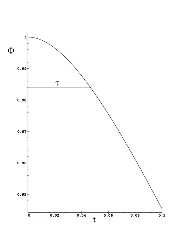
Figure 1: The time dependent correlation $\Phi\left(t\right)=const\left[\frac{e^{-\nu t}}{\nu}-\frac{e^{-bt}}{b}\right]$ for the ratio $\frac{b}{\nu}=20$.

for $1/l\;<<\;\tau\;<<1/\nu.$ This is described in figure 1

SHOW FIGURE 1 HERE.

In the limit $l\rightarrow\infty$, the Fokker-Planck equation for the probability of finding $h$ at $t$ satisfies:

$$\left[\frac{\partial}{\partial t}-\frac{\partial}{\partial h}\left(D_{0}\frac{\partial}{\partial h}+\nu h\right)\right]P=0,$$ (2.10)

which gives

$$\frac{\partial\Phi}{\partial t}+\nu\Phi=0\;\;\;\;t>0$$ (2.11)

and

$$-\frac{\partial\Phi}{\partial t}+\nu\Phi=0\;\;\;\;t<0$$ (2.12)

and $\Phi\left(0\right)=D_{0}/\nu$. The awkwardness of (2.8)-(2.12) is removed by putting in the full dependence on $l$, but more simply, as described above, confining ourselves to $t>0$,we have the first order differential equation (2.11) with the initial condition $\Phi\left(0\right)=D_{0}/\nu$, that implies a finite derivative $\dot{\Phi}\left(0\right)=-D_{0}$ at $t=0$. This matches the static equation obtained from the Fokker-Planck equation (2.10)

$$D_{0}-\nu\left<hh\right>=0$$ (2.13)

The form of the Fourier transform of $\Phi\left(t\right)$, $\Phi\left(\omega\right)$, suggests the structure of $\Phi_{k,\omega}$ in the non-linear field theory.

For the simple linear case,

$$\Phi_{\omega}=\frac{H/\pi}{[\omega^{2}+\nu^{2}][\omega^{2}+l^{2}]}\equiv\frac{H/\pi}{\Omega^{*}\Omega},$$ (2.14)

where $\Omega=[i\omega+\nu][i\omega+l]$.

Thus the two decays of $\Phi(t)$, for $t>0$, are present as zeroes of $\Omega$ (poles in $\Phi_{\omega}$, in the upper half of the complex $\omega$ plane.) In the limit $l\rightarrow\infty$, the situation is similar, but there is only a single decay

$$\Phi_{\omega}=\frac{D_{0}}{\omega^{2}+\nu^{2}}=\frac{D_{0}/\pi}{\Omega^{*}\Omega},$$ (2.15)

where $\Omega=[i\omega+\nu]$.

The natural model to try for the $\Phi$ of the non-linear equation is [7]

$$\Phi_{{\bf k}\omega}=\frac{D_{{\bf k}\omega}}{\Omega_{{\bf k}\omega}\Omega^{*}_{{\bf k}\omega}},$$ (2.16)

where $D_{{\bf k}\omega}=D_{-{\bf k},-\omega}>0$ with no singularities in the complex $\omega$ plane, and where $\Omega$ gives in the first self consistent approximation a simple decay described by

$$\Omega_{{\bf k}\omega}=i\omega+\omega_{\bf{k}}\,.$$ (2.17)

However, there will be a much more complicated time dependence in the full $\Phi$ than one simple decay. (Equations (2.14) and (2.15) form a simple example where the decay is given to first approximation by a simple decay but indeed the behaviour is more complicated)

One possible definition of $\Omega$ is to use the response function and define $\Omega$ by

$$\frac{D_{0}}{\Omega_{{\bf k}\omega}}=\left<f_{-{\bf k}-\omega}h_{{\bf k}\omega}\right>$$ (2.18)

and employed in mode-mode coupling studies [5, 15, 16]. We will take the view that we can write $\Phi$ in terms of a sum of exponential decays which can be extended to cover continuous distributions i.e. branch cuts rather than simple poles. Confining ourselves to poles for the moment, if we write

$$\Phi_{{\bf k}\omega}=\sum_{\bf l}\frac{A_{l,{\bf k}}}{\omega^{2}+\omega^{2}_{{\bf k},{\bf l}}}=\frac{D_{{\bf k}\omega}}{\Pi_{\bf l}\left(\omega^{2}+\omega^{2}_{{\bf k},{\bf l}}\right)},$$ (2.19)

we find that $D_{{\bf k}\omega}$ is an even function in $\omega$ (a polynomial for a finite sum of simple decays), and it has no singularities.

Thus

$$\Omega_{{\bf k}\omega}=\frac{1}{\prod_{\bf l}\left(i\omega+\omega_{{\bf k},{\bf l}}\right)}$$ (2.20)

and

$$\Omega^{*}_{{\bf k}\omega}=\frac{1}{\prod_{\bf l}\left(-i\omega+\omega_{{\bf k},{\bf l}}\right)}$$ (2.21)

When $\Phi_{{\bf k}}\left(t\right)$ is obtained from (2.19) only the poles $\omega=i\omega_{{\bf k},l}$ contribute to $t>0$ and their conjugates for $t<0$.

The strategy we will adopt is to construct a transport equation for $\Phi_{{\bf k}\omega}$ in which the first order approximation (2.17) for $\Omega_{{\bf k}\omega}$ will be useful and it will result in a higher order approximation for $\Phi_{{\bf k}\omega}$ and consequently for $\Phi_{{\bf k}}\left(t\right)$ that will show now a decay that is much more complicated than a simple exponential.

3 The expansion

The starting point is equation (1.5), where in order to make our notation less cumbersome, we denote the $d+1$ vector $({\bf k},\omega)$ by ${\bf K}$ and write the equation in the form

$$\Omega_{0{\bf K}}h_{{\bf K}}+\sum M_{{\bf{\bf kjl}}}h_{{\bf J}}h_{{\bf L}}-f_{{\bf K}}={\bf 0}$$ (3.1)

We define next $P\left\{h_{{\bf K}};f_{{\bf K}}\right\}$ to be the distribution of the $h_{{\bf K}}$’s in the presence of a given noise, $f_{{\bf K}}$. $P$ is to be averaged eventually over the noise. The Liouville equation (1.6) is now replaced by

$$\left[\Omega_{0{\bf K}}h_{{\bf K}}+\sum_{{\bf JL}}M_{{\bf{\bf kjl}}}h_{{\bf J}}h_{{\bf L}}-f_{{\bf K}}\right]P=0$$ (3.2)

which is similar to a Fermi supplementary condition. Equivalently, equation (3.2) can be replaced by:

$$\sum_{{\bf K}}\frac{\partial}{\partial h_{{\bf K}}}\left(\Omega_{0{\bf K}}h_{{\bf K}}+\sum_{{\bf JL}}M_{{\bf{\bf kjl}}}h_{{\bf J}}h_{{\bf L}}-f_{{\bf K}}\right)P=0,$$ (3.3)

to obtain the correct hierarchy of field correlations. This is achieved by multiplying the above equation by products like $h_{{\bf L}1}...h_{{\bf L}N}$ and integrating by parts. A simple example is obtained by multiplication by $h_{{\bf K}}$ that yields the correct average of equation (3.1).

$$\Omega_{0{\bf K}}\left<h_{{\bf K}}\right>+\sum_{{\bf J},{\bf L}}M_{{\bf{\bf kjl}}}\left<h_{{\bf J}}h_{{\bf L}}\right>-f_{{\bf K}}=0.$$ (3.4)

An alternative derivation of equation (3.3) starts with consideration of a $d+2$ dimensional system in which the equation of the form

$$\frac{\partial}{\partial s}h_{{\bf K}}(s)=\left[\Omega_{0{\bf K}}h_{{\bf K}}(s)+\sum_{{\bf JL}}M_{{\bf JKL}}h_{{\bf J}}(s)h_{{\bf L}}(s)-f_{{\bf K}}+g_{{\bf K}}(s)\right]$$ (3.5)

is considered, where $g_{{\bf K}}(s)$ is a $d+2$ dimensional noise obeying

$$<g_{{\bf K}}(s)>=0\;and\;<g_{{\bf K}}(s)g_{-{\bf K}}(s^{\prime})>={\mathcal{D}}_{{\bf K}}\delta(s-s^{\prime}).$$ (3.6)

(Note that $f_{{\bf K}}$ does not depend on $s$. Therefore it plays the role of quenched randomness). The Fokker-Planck equation for ${\mathcal{P}}\left\{h_{{\bf K}},s\right\}$, the distribution of a given configuration $\left\{h_{{\bf K}}\right\}$ is given by

$$\frac{\partial{\mathcal{P}}}{\partial s}=\sum_{{\bf K}}\frac{\partial}{\partial h_{{\bf K}}}\left[{\mathcal{D}}_{{\bf K}}\frac{\partial}{\partial h_{-{\bf K}}}+\Omega_{0{\bf K}}h_{{\bf K}}+\sum_{{\bf JL}}M_{{\bf{\bf kjl}}}h_{{\bf J}}h_{{\bf L}}-f_{{\bf K}}\right]{\mathcal{P}}.$$ (3.7)

The ’steady state’ ($s$ independent) $\mathcal{P}$ in the limit where ${\mathcal{D}}_{{\bf K}}$ is zero is the distribution of $h_{{\bf K}},P$ and equation (3.3) is recovered.

In order to construct an expansion for $P$, we write equation (3.3) as:

$$\sum_{{\bf K}}\frac{\partial}{\partial h_{\bf K}}\left(\frac{{\mathcal{D}}_{{\bf K}}}{\Omega_{-{\bf K}}}\frac{\partial}{\partial h_{\bf-K}}+\Omega_{{\bf K}}h_{{\bf K}}\right)+\sum_{{\bf K}}\frac{\partial}{\partial h_{{\bf K}}}\left[\sum_{{\bf JL}}M_{{\bf{\bf kjl}}}h_{{\bf J}}h_{{\bf L}}-f_{{\bf K}}\right]\\ +\sum_{{\bf K}}\frac{\partial}{\partial h_{{\bf K}}}\left[\left(\Omega_{0{\bf K}}-\Omega_{{\bf K}}\right)h_{{\bf K}}-\frac{{\mathcal{D}}_{{\bf K}}}{\Omega_{-{\bf K}}}\frac{\partial}{\partial h_{-{\bf K}}}\right]P=0$$ (3.8)

Notice that since the sum is over all $\bf K$, both $\Omega_{{\bf K}}$ and $\Omega_{-{\bf K}}$ will appear in the second derivative.

We expect an expansion, of the average of $P$ over the noise, around the Gaussian

$$P_{0}\propto{\rm exp}\left[-\frac{1}{2}\sum_{{\bf K}}\frac{h_{{\bf K}}h_{-{\bf K}}}{\Phi_{{\bf K}}}\right]$$ (3.9)

and, as before, associate in (3.8) a notional $\lambda$ to the second term on the left hand side of equation (3.9) and $\lambda^{2}$ to the third term. Expanding to second order in the $\lambda$ ”Chapman and Enskog” expansion, we get

$$P=P_{0}\left(1-\sum_{{\bf{\bf kjl}}}\frac{M_{{\bf{\bf kjl}}}h_{{\bf J}}h_{{\bf L}}h_{-{\bf K}}}{\left[\Omega_{{\bf J}}+\Omega_{{\bf L}}+\Omega_{-{\bf K}}\right]\Phi_{{\bf K}}}+...\right)$$ (3.10)

The condition that $<h_{{\bf K}}h_{-{\bf K}}>$ calculated to second order in $\lambda$ is equal to $\Phi_{{\bf K}}$ (that is the zero order result) yields an equation for $\Phi$ in terms of $\Omega$.

$$\frac{1}{2}\left(\Omega_{0{\bf K}}+\Omega_{0,{\bf-K}}\right)\Phi_{{\bf K}}-2\sum_{{\bf JL}}\frac{M_{{\bf{\bf kjl}}}M_{{\bf JK,-L}}}{\left[\Omega_{{\bf J}}+\Omega_{{\bf L}}+\Omega_{-{\bf K}}\right]}\Phi_{{\bf L}}\Phi_{{\bf K}}-\\ \sum_{{\bf JL}}\frac{|M_{{\bf{\bf kjl}}}|^{2}}{\left[\Omega_{{\bf J}}+\Omega_{{\bf L}}+\Omega_{-{\bf K}}\right]}\Phi_{{\bf J}}\Phi_{{\bf L}}=\frac{D_{0}}{2}\left[\frac{1}{\Omega_{{\bf K}}}+\frac{1}{\Omega_{-{\bf K}}}\right].$$ (3.11)

We can recover the structure of a transport equation, familiar from the static case, i.e. ”un-pick” $\Omega_{0{\bf K}}+\Omega_{0,-{\bf K}}$ and $1/\Omega_{{\bf K}}+1/\Omega_{-{\bf K}}$ by returning to equation (3.1), multiplying it by $h_{-{\bf K}}$ and averaging over the distribution (3.10). Using also equation (2.18) we obtain

$$\Omega_{0{\bf K}}\Phi_{{\bf K}}-2\sum_{{\bf JL}}\frac{M_{{\bf{\bf kjl}}}M_{{\bf JK,-L}}}{\left[\Omega_{{\bf J}}+\Omega_{{\bf L}}+\Omega_{-{\bf K}}\right]}\Phi_{{\bf L}}\Phi_{{\bf K}}-\sum_{{\bf JL}}\frac{|M_{{\bf{\bf kjl}}}|^{2}}{\left[\Omega_{{\bf J}}+\Omega_{{\bf L}}+\Omega_{-{\bf K}}\right]}\Phi_{{\bf J}}\Phi_{{\bf L}}=\frac{D_{0}}{\Omega_{-{\bf K}}}.$$ (3.12)

At this point we use, just in the non linear term, the first order approximation $\Omega_{{\bf K}}=i\omega+\omega_{{\bf K}}$. This has the advantage that now $\Omega_{{\bf J}}+\Omega_{{\bf L}}+\Omega_{-{\bf K}}=\omega_{\bf j}+\omega_{\bf l}+\omega_{\bf k}$. Fourier transforming back and recalling that the zeroes of $\Omega_{-{\bf K}}$ are in the lower complex $\omega$ plane, we find for $t>0$ the local equation

$$\frac{\partial\Phi_{\bf k}(t)}{\partial t}+\nu_{\bf k}\Phi_{\bf k}(t)-2\sum\frac{M_{{\bf{\bf kjl}}}M_{\bf{jk},-\bf{l}}}{\omega_{\bf j}+\omega_{\bf l}+\omega_{\bf k}}\phi_{\bf l}\Phi_{\bf k}(t)-\\ \sum\frac{|M_{\bf{{\bf kjl}}}|^{2}}{\omega_{\bf j}+\omega_{\bf l}+\omega_{\bf k}}\Phi_{\bf j}(t)\Phi_{\bf l}(t)=0$$ (3.13)

and

$$-\frac{\partial\Phi_{\bf k}(t)}{\partial t}+\nu_{\bf k}\Phi_{\bf k}(t)-2\sum\frac{M_{{\bf kjl}}M_{\bf{jk},-\bf{l}}}{\omega_{\bf j}+\omega_{\bf l}+\omega_{\bf k}}\phi_{\bf l}\Phi_{\bf k}(t)-\\ \sum\frac{|M_{{\bf kjl}}|^{2}}{\omega_{\bf j}+\omega_{\bf l}+\omega_{\bf k}}\Phi_{\bf j}(t)\Phi_{\bf l}(t)=0\;\mbox{for}\;t<0.$$ (3.14)

Notice that the above is possible because the coefficients, $M_{{\bf{\bf kjl}}}$, do not depend on the fourth components of the vector. The initial conditions with which equation (3.13) has to be solved are

$$\Phi_{\bf k}(0)=\phi_{\bf k},\quad\mbox{for all k,}$$ (3.15)

where $\phi_{\bf k}$ is the static correlations. The static equation determining $\phi_{\bf k}$ is

$$\nu_{\bf k}\phi_{\bf k}-2\sum\frac{M_{{\bf kjl}}M_{\bf{jk},-\bf{l}}}{\omega_{\bf j}+\omega_{\bf l}+\omega_{\bf k}}\phi_{\bf l}\phi_{\bf k}-\sum\frac{|M_{{\bf kjl}}|^{2}}{\omega_{\bf j}+\omega_{\bf l}+\omega_{\bf k}}\phi_{\bf j}\phi_{\bf l}=_{{\bf k}0}.$$ (3.16)

It can be shown that

$$\lim_{t\to 0+}\frac{\partial\Phi_{\bf k}(t)}{\partial t}=-_{{\bf k}0},$$ (3.17)

is an exact relation, obeyed by the exact two point function. Using this general result, we see that as $t\rightarrow 0+$, the evolution equation for $\Phi_{\bf k}(t)$, eq. (3.13) fits exactly onto the static equation for $\phi_{\bf k}$, eq. (3.16). The equations (3.13) and (3.16) were originally derived for the driven Navier-Stokes equations [7], but although equation (3.13) can give the Kolmogoroff [17] spectrum with a good value for the front factor, the boundary condition was not understood at that time, and this hindered further development of this approach to non-linear equations by this route for several decades. Note that the simplicity of the basic equations (3.13-3.15) and (3.16) sets this approach apart from mode-mode coupling theories. We have found a plausible way (the structure of $\Omega$) which leads to these manageable and transparent equations. The amazing feature of the self-consistent approach is that the time-dependent equation has an explicit and local dependence in time. It now offers a way to complete the system of functions, $\phi_{\bf{k}}$, $\omega_{\bf{k}}$ in a satisfying way. To the best of our knowledge the direct evaluation of the indices of $\phi_{\bf{k}}$ and $\omega_{\bf{k}}$ and the universal structure of the time dependent correlation functions are not available from other treatments. The simple structure of our equations now offers a way to complete the system of functions, $\phi_{\bf k},\omega_{\bf k}$, in a satisfying way. We define $\omega_{\bf k}$ customarily to be given by

$$\omega_{\bf k}^{-1}=\frac{\int_{0}^{\infty}\Phi_{\bf k}(t)\;{\rm d}t}{\phi_{\bf k}},$$ (3.18)

which is a natural definition, if we think about a single mode decay. Integrating equation (3.13) over time, taking into account (3.17) and the fact that $\int_{0}^{\infty}\frac{\partial\Phi_{\bf k}(t)}{\partial t}\;{\rm d}t=-\phi_{\bf k}$, we obtain

$$\omega_{\bf k}=\nu_{\bf k}-2\sum_{j,l}\frac{M_{{\bf kjl}}M_{\bf{jk},-\bf{l}}}{[\omega_{\bf j}+\omega_{\bf l}+\omega_{\bf k}]}\phi_{\bf l}-\sum\frac{|M_{{\bf kjl}}|^{2}}{[\omega_{\bf j}+\omega_{\bf l}+\omega_{\bf k}]}\times\\ \frac{\phi_{\bf j}\phi_{\bf l}}{\phi_{\bf k}}\left(\frac{\omega_{\bf k}}{\omega_{\bf{j},\bf{l}}}\right)\,,$$ (3.19)

where

$$\int_{0}^{\infty}\Phi_{\bf l}(t)\Phi_{\bf j}(t)\;{\rm d}t=\frac{\phi_{\bf l}\phi_{\bf j}}{\omega_{\bf{j},\bf{l}}}\,.$$ (3.20)

Neglecting $D_{0k}$ and $\nu_{\bf k}$ in equation (3.16) (the static equation) and (3.19) (the $\omega$ equation) we find that in the inertial range

$$\omega_{\bf k}\,=\,\sum\,\frac{|M_{{\bf kjl}}|^{2}\,\phi_{\bf j}\phi_{\bf l}\,(\omega_{\bf{j},\bf{l}}\,-\,\omega_{\bf k})}{(\omega_{\bf k}\,+\,\omega_{\bf j}\,+\,\omega_{\bf l})\,\phi_{\bf k}\,\omega_{\bf{j},\bf{l}}}$$ (3.21)

A similar equation has been derived by a different method by Edwards and McComb [9], who used it to derive the Kolmogoroff front factor, achieving a reasonable value. Details of the alternative method are given in the book of McComb [17]. It is easy to see that eq.(3.19) leads just to the scaling relation discussed in the introduction because $\omega_{\bf{j},\bf{l}}$ scales as $\omega$. This scaling relation together with the static equation gives

$$\omega_{\bf k} = B_{1}k^{3/2}\;\mbox{in KPZ in 1+1 D}$$

$$= B_{2}k^{1.7}\;\mbox{in KPZ in 2+1 D [2]}$$

$$\omega_{\bf k} = B_{3}k^{2/3}\;\mbox{in KNS [13]}$$

4 A closer look at the steady state in the inertial range

The structure of the steady state equation has the form

$$\int\Lambda^{(1)}(j,k)\phi_{\bf j}\phi_{\bf k}\;{\rm d}^{d}j-\int\Lambda^{(2)}(j,k)\phi_{\bf j}\phi_{\bf{k}-\bf{j}}\;{\rm d}^{d}j=_{{\bf k}0}-\nu_{\bf k}\phi_{\bf k}.$$ (4.1)

The kernel $\Lambda^{(2)}$ stemming from the $|M_{{\bf kjl}}|^{2}$ term is positive definite but $\Lambda^{(1)}(j,k)$ may attain positive as well as negative values depending on the specific problem and the values of $j$ and $k$. For $KPZ$ with noise, that is white (in space) it was shown explicitly [10] that the exponent characterising the leading small $k$ dependence is obtained by equating the left hand side of eq. (4.1) to zero. The concept of inertial range is given thus a definite meaning since the exponent does not depend neither on the source nor the ’viscosity’. For $KPZ$ with noise given by ${}_{{\bf k}0}=D_{0}k^{-2\rho}$ [18] it was shown that up to some threshold $\rho_{0}$ the inertial range still exists and the exponent characterising the small $k$ behaviour does not depend on the source or the ’viscosity’ (and therefore, its value is the same as in the white noise case). For $\rho>\rho_{0}$, the system is driven by the noise and even the leading $k$ dependence depends on the source term. The problem of turbulence seems to combine both behaviours in an interesting way. The simplest conceptual picture of the inertial range is that offered by Kolmogoroff, where random forces put energy into a fluid at low $\bf{k}$, and viscosity removes it at high $\bf{k}$. We can make an extreme model of this by taking the input to be $\varepsilon\delta\left({\bf{k}}\right)$ and the output to be $\varepsilon\frac{\delta\left(\left|\bf{k}\right|-\infty\right)}{4\pi\left|\bf{k}\right|^{2}}$ which we write symbolically as $\varepsilon\delta\left(k-\infty\right)$, so that

$$\int\Lambda^{\left(1\right)}\phi_{{\bf{k}}}\phi_{{\bf{j}}}\;d^{3}{\bf{j}}-\int\Lambda^{\left(2\right)}\phi_{{\bf{k-j}}}\phi_{{\bf{j}}}\;d^{3}{\bf{j}}=\varepsilon\left[\delta\left(k\right)-\delta\left(k-\infty\right)\right].$$ (4.2)

The Navier Stokes $\mathcal{M}$ guarantees that the integral over $\bf{k}$ of the left hand side vanishes for any $\phi_{\bf k}$

$$\int\left(\int\Lambda^{\left(1\right)}\phi_{{\bf{k}}}\phi_{{\bf{j}}}\;d^{3}{\bf{j}}-\int\Lambda^{\left(2\right)}\phi_{{\bf{k-j}}}\phi_{{\bf{jh}}}\;d^{3}{\bf{j}}\right)\;d^{3}{\bf{k}}=0$$ (4.3)

and so matches

$$\int d^{3}{\bf{k}}\;\varepsilon\left[\delta\left(k\right)-\delta\left(k-\infty\right)\right]=0\,.$$ (4.4)

To clarify (4.2)-(4.4) we offer a model in Appendix B.

We have computed the value of the left hand side of equation (4.2) for a range of values of $\Gamma$, and calling the quantity $Z\left(\Gamma\right)$, we find that the value of $\Gamma$ for which $Z\left(\Gamma\right)=0$ is (see figure 2)

$$\Gamma=3.6667$$ (4.5)

to the accuracy of our computation (For $KPZ$, we have already found the value 2.59).

show figure 2 here

We have used the $\phi_{\bf k}=k^{-11/3}$ and integrated the left hand side of eq.(4.2) over a finite $k$ sphere, interchanging the $k$ and $j$ integration, we obtain, as expected, a non-zero result, in spite of the fact that for any finite $k$ the integrand is zero.

This results gives one the confidence to proceed to the much more difficult problem of the time dependence.

It is interesting to consider briefly another example which is Navier-Stokes driven white noise (call it $WNS$). In the problem, the viscosity can again only influence very large $k$, but now the source plays a vital part. Integrals converge, with the solution of

$$\int\Lambda^{(1)}\phi_{\bf k}\phi_{\bf j}-\int\Lambda^{(2)}\phi_{\bf{k}-\bf{j}}\phi_{\bf j}=D_{0}$$ (4.6)

where $D_{0}$ is now a constant, and one finds

$$\phi_{\bf k} \propto Ek^{-5/3}D_{0}^{2/3},\;\mbox{and}$$

$$\omega_{\bf k} \propto Fk^{5/3}D_{0}^{1/3}\;$$

If one tried to solve this in the $KPZ$ style of ignoring $D_{0}$, one would of course get Kolmogoroff again, but Kolmogoroff’s $-11/3$, $2/3$ regime will not satisfy equation(4.6).

5 The time dependent correlation function

So far we have obtained the solution for the steady state correlation function, $\left<h_{{\bf{k}}}\left(t\right)h_{{\bf{-k}}}\left(t\right)\right>$ in the two cases of $KPZ$ and $NS$. Turning to the time dependent function, $\Phi_{{\bf{k}}}\left(t\right)$, at first sight we are faced with a formidable set of equations, given by (3.13), (3.16) and (3.19), of which (3.13) is central.We give firstly a crude argument and relegate a full discussion to Appendix C. If we write $\Phi_{\bf k}~{}=~{}\phi_{\bf k}e^{-\Gamma_{\bf k}(t)}$ we can manipulate (3.13) and (4.1) to obtain

$$\frac{\partial\Gamma_{\bf k}}{\partial t}\,=\,\int\,\Lambda_{2}\,\frac{\phi_{\bf j}\,\phi_{\bf{k}-\bf{j}}}{\phi_{\bf k}}\,\Big{(}1\,-\,e^{-\Gamma_{\bf j}(t)-\Gamma_{\bf{k}-\bf{j}}(t)+\Gamma_{\bf k}(t)}\Big{)}\,\mbox{d}^{3}j\,,$$ (5.1)

and argue (to be justified at greater length in Appendix C) the solution is dominated by the that part of $j$ space where

$$1\,=\,e^{-\Gamma_{\bf j}-\Gamma_{\bf{k}-\bf{j}}+\Gamma_{\bf k}}$$ (5.2)

i.e. $\Gamma_{\bf j}(t)+\Gamma_{\bf{k}-\bf{j}}(t)~{}=~{}\Gamma_{\bf k}(t)$. We can scale out $t$ and have

$$\Gamma_{\bf j}+\Gamma_{\bf{k}-\bf{j}}\,=\,\Gamma_{\bf k}$$ (5.3)

where $\Gamma_{\bf k}~{}=~{}\Gamma_{\bf k}(1)$ etc.. Consider this guess: $\Gamma_{\bf k}~{}\sim~{}k^{2}$. Then we would need $k^{2}~{}=~{}(\bf{k}+\bf{j})^{2}+j^{2}$ which by Pythagoras’s theorem gives the locus of $j$ to be a sphere of diameter $k$. Inside the sphere

$$\Gamma_{\bf k}\,>\,\Gamma_{\bf{k}-\bf{j}}\,+\,\Gamma_{\bf j}$$ (5.4)

Outside the sphere

$$\Gamma_{\bf k}\,<\,\Gamma_{\bf{k}-\bf{j}}\,+\,\Gamma_{\bf j}$$ (5.5)

so the guess is inadequate. The only way to find a region of $j$ space wherein (5.3) obtains is when $\Gamma$ is linear when $\bf{j}$ equals $\alpha\bf{k}$ such that $1~{}\geqslant~{}\alpha~{}\geqslant~{}0$. The integral goes outside that locus, but the corrections are logarithmic and derived in Appendix C. Returning to $\Gamma_{\bf k}(t)$

$$\Gamma_{\bf k}(t)\,=\,a\,|\bf{k}|\,t^{1/\mu}$$ (5.6)

where $a$ is a constant of the appropriate dimensions. For $\mu~{}>~{}1$, we derive in Appendix C the long time decay of $\Phi_{\bf k}(t)$, including the logarithmic corrections

$$\Phi_{\bf k}(t)\,\varpropto\,\Big{(}a\,|\bf{k}|\,t^{1/\mu}\Big{)}^{\frac{d-1}{2}}\,exp(-a\,|\bf{k}|\,t^{1/\mu})\,.$$ (5.7)

6 Some speculations

Working to a kernel of order $M^{2}$, the ”transport” equation we have derived has the classic form with operators $A$, $B$ such that

$$A\phi+B\phi\phi=D;$$ (6.1)

but the solutions for different physical cases seem radically different.

For $KPZ$, it appears that $A$ and $D$ are not central to the inertial range away from $k=0$ and $k=\infty$, and the solution is given by taking a power law $k^{-\Gamma}$, and deriving in detail

$$B\phi\phi=Z\left(\Gamma\right)$$ (6.2)

so that the value of $\Gamma$ must be such that

$$Z\left(\Gamma\right)=0$$ (6.3)

and this gives the solution in the inertial range. The solution is then improved by adding the effects of $A\phi$ and $D$. However, for problems rich in dimensional parameters, e.g. instead of $M_{{\bf{{\bf kjl}}}}$ being a combination of powers, it could be a function like $\rm{e}^{-\left(k^{2}+\left({\bf{k}}+{\bf{j}}\right)^{2}+j^{2}\right)c^{2}}$, containing a new constant $c$ with dimensions (length), likewise for $A$ and $D$, then equation 6.1 is more of a standard Boltzmann form and, for example, a perturbation approach would be

$$\phi=\frac{D}{A}-B\frac{D}{A}\frac{D}{A}+\cdots$$ (6.4)

which can be improved in various ways. Navier-Stokes seems to have aspects of both of these, for at first sight, if one tries a power, then $B\phi\phi=0$ has the Kolmogoroff solution derived just as the $KPZ$ is derived. In fact the lack of uniform convergence puts Kolmogoroff into the form:

$$B\phi\phi=D$$ (6.5)

and the $A\phi$ term only comes in to polish the solution at high $k$. For $WNS$ an attempt to use (6.3) inevitably gives the Kolmogoroff indices which are quite incorrect for this problem. One must use (6.5) since $D$ is a constant for all $\bf k$, not just being non-zero at $k=0$ as in $KNS$.

Suppose now that we proceed to the next orders, which will give

$$A\phi+B\phi\phi+C\phi\phi\phi+E\phi\phi\phi\phi+\cdots=D$$ (6.6)

Can we now try $\phi\sim k^{-\Gamma}$ and obtain

$$Z_{B}\left(\Gamma\right)+Z_{C}\left(\Gamma\right)+Z_{E}\left(\Gamma\right)+\cdots=0.$$ (6.7)

For $KPZ$, $Z_{B}\left(\Gamma\right)=0$ gives a $\Gamma$ which cannot be obtained from dimensional analysis. More detail is given in Appendix D. There is no reason to believe that if we proceeded to equation (6.7) it will not give again a $\Gamma$, not quite the same as that of equation (6.2), but if the self consistent approach works well it will be close. Certainly numerical simulations equivalent to all orders in (6.6) do agree remarkably well with the second order, (6.2). However, in other equations, in particular $KNS$, the deficiency in dimensions of the equations leads to the Kolmogoroff solution both by looking at $Z_{B}\left(\Gamma\right)=0$, and by balancing the source term with the energy cascade. What happens if we go to the higher orders in $KNS$? Could it be that equation (6.7) has a non Kolmogoroff solution? The calculation of $C,E$ etc. in equation (6.6) is a formidable undertaking and, unless some new dimensional quantity is needed to make $C,E$ convergent, there seems to no reason that Kolmogoroff should not again be the solution.

7 Acknowledgements

S.F.E. acknowledges with gratitude the award of a senior research fellowship from the Leverhulme Foundation, and for support from the Polymers and Colloids Group at the Cavendish Laboratory, and from the Sackler Foundation at Tel Aviv University.

M.S. acknowledges support from the Sackler Foundation at the Sackler Institute at Tel Aviv University, and the Polymers and Colloids Group at the Cavendish Laboratory, Cambridge University.

8 Appendices

Appendix A

In quantum field theory the algebraic series which, in for example the basic papers of Schwinger [19], can be rather impenetrable, becomes much simpler with the use of Feynman diagrams. In this paper, we are proposing that the Boltzmann equation is the correct target for equations like $KPZ$, we should offer a graphology to simplify the appreciation of the formal expansion. This has in fact been done in the original study of $NS$ many years ago [7, 17], and extended to many body problems by Sherrington [20], and then fully extended to turbulence problems [21]. However, it is not well known and so we reproduce it here, and extend the analysis to some new cases, in particular the expressions for fourth moments. We use the notation of the steady state problem, although it works equally for the time dependent case. The problem is to find $P$ which satisfies (1.8). $P$ is to be expanded about $P_{0}$, which satisfies (1.9), and this is effected by introducing $D$ and $\omega$, so that writing

$$\Delta D = D-D_{0}$$ (A.1)

$$\mbox{and}\;\;\Delta\omega = \omega-\nu$$ (A.2)

$$\frac{\partial}{\partial h}\left(D\frac{\partial}{\partial h}+\omega h-\Delta D\frac{\partial}{\partial h}-\Delta\omega h+Mhh\right)\left(P_{0}+P_{1}+P_{2}\cdots\right)=0$$ (A.3)

and ascribing $"\lambda"$ to $Mhh$ and $"\lambda^{2}"$ to $\Delta D$ and $\Delta\omega$, we expand

$$P = P_{0}+P_{1}+P_{2}+\cdots$$ (A.4)

$$P_{1} = G\frac{\partial}{\partial h}MhhP_{0}$$

$$P_{2} = G\frac{\partial}{\partial h}MhhG\frac{\partial}{\partial h}MhhP_{0}$$

$$+ G\bigg{(}\frac{\partial}{\partial h}\Delta D\frac{\partial}{\partial h}+\frac{\partial}{\partial h}\Delta\omega h\bigg{)}P_{0}\,,$$

where G is the Green function defined in (A.6) below. To evaluate $P_{1}$, $P_{2}$, $\cdots$ we are repeatedly faced with the problem of finding J, where

$$\int Gk_{abc\dots}h_{a}^{\prime}h_{b}^{\prime}h_{c}^{\prime}\dots P_{0}^{\prime}\Pi\;dh^{\prime}=J\left(h\right)$$ (A.5)

or since symbolically

$$\sum\frac{\partial}{\partial h}\left(D\frac{\partial}{\partial h}+\omega h\right)G=\Pi\delta$$ (A.6)

and defining $\widetilde{G}$ by

$$Khhh\dots P_{0}=\frac{\partial}{\partial h}\left(D\frac{\partial}{\partial h}+\omega h\right)JP_{0}\\ =P_{0}\left(D\frac{\partial}{\partial h}-\omega h\right)\left(-\frac{\partial}{\partial h}\right)J=P_{0}\widetilde{G}J$$ (A.7)

we will show that the significant problem (significant to order $V^{-1}$ relative to other terms), is when $K_{abc\dots}h_{a}h_{b}h_{c}\dots$ has none of $a,\,b,\,c,\,\dots$ paired i.e. $b,\,c\,\dots\neq-a$. Then we try $J={\cal J}_{abc}h_{a}h_{b}h_{c}\dots$ we find a solution provided

$${\cal J}_{abc\dots}=\omega_{a}+\omega_{b}+\omega_{c}+\dots$$ (A.8)

by direct substitution. The second derivative always gives zero, and

$$\omega_{a}h_{a}\frac{\partial}{\partial h_{a}}h_{a}=\omega_{a}h_{a}$$ (A.9)

If ever we do find $h_{\bf l}h_{-l}$ we replace it by $\phi_{\bf l}+\left(h_{\bf l}h_{-l}-\phi_{\bf l}\right)$ and the bracketed term, as in all field theories leads only to terms of order $V^{-1}$. Thus as the series develops, a term in $h$ adds an $h$, $a\frac{\partial}{\partial h}$ removes an $h$, a $G$ inserts a term like $\sum\omega$ for each $h$. The first correction to $P_{0}$, $P_{1}$, illustrates the process:

$$P_{1}=\sum GM_{{\bf{{\bf kjl}}}}h_{{\bf{j}}}h_{{\bf{l}}}\frac{\partial}{\partial h_{{\bf{k}}}}P_{0}$$ (A.10)

$$= -\sum\left[GM_{{\bf{{\bf kjl}}}}h_{{\bf{j}}}h_{{\bf{l}}}h_{{\bf{-k}}}/\phi_{{\bf{k}}}\right]P_{0}$$

$$= -\sum P_{0}\tilde{G}M_{{\bf{{\bf kjl}}}}h_{{\bf{j}}}h_{{\bf{l}}}h_{{\bf{-k}}}/\phi_{{\bf{k}}}$$ (A.11)

$$= -\sum P_{0}\left(\frac{M_{{\bf{{\bf kjl}}}}h_{{\bf{-k}}}h_{{\bf{j}}}h_{{\bf{l}}}/\phi_{{\bf{k}}}}{\omega_{{\bf{k}}}+\omega_{{\bf{j}}}+\omega_{{\bf{l}}}}\right).$$ (A.12)

Suppose that we wanted the value of $\left<h_{a}h_{b}h_{c}\right>$, then it is given to order $M$ by

$$-\frac{M_{{\bf{{\bf kjl}}}}\phi_{{\bf{j}}}\phi_{{\bf{l}}}}{\omega_{{\bf{k}}}+\omega_{{\bf{j}}}+\omega_{{\bf{l}}}}\left[\delta_{\bf{k},-\bf{a}}\delta_{\bf{j},-\bf{b}}+\mbox{permutations}\right].$$ (A.13)

(Note that $M$ has $\delta_{\bf{k},\bf{j}+\bf{l}}$) At this point we introduce the diagrams. Draw these pictures:

$$\frac{\partial}{\partial h_{{\bf{k}}}}Mh_{{\bf{j}}}h_{{\bf{l}}} =$$ (A.14)

$$\frac{\partial}{\partial h_{\bf k}}\frac{\partial}{\partial h_{-k}}D_{0} =$$

$$\frac{\partial}{\partial h_{\bf k}}\frac{\partial}{\partial h_{-k}}\Delta D =$$

$$\frac{\partial}{\partial h_{\bf k}}\nu_{\bf k}h_{\bf k} =$$

$$\frac{\partial}{\partial h_{\bf k}}h_{\bf k}\Delta\omega =$$

The rippled line will always point in the direction to the left, for in final evaluations integration by parts gives non-zero values only when the $\frac{\partial}{\partial h}$ finds an $h$ to its left. The full lines representing $h$ can point left or right. Note that $\omega_{{\bf k}}=\omega_{-{\bf k}}$ and that as in normal field theories, strictly speaking arrows need to be attached to the lines.

Our problem now is:

$$\left(\raisebox{-27.89998pt}{\includegraphics[height=61.99997pt]{7_21.eps}}\right)P=0$$ (A.17)

Upon integration, $P_{0}$ joins $\bf k$ and $-\bf k$ to give the line

$$\raisebox{-20.46pt}{\includegraphics[height=30.99998pt]{7_22.eps}}=\phi_{\bf k}$$ (A.18)

Thus our series for $P$ is

$$P=\Bigg{(}\raisebox{-61.99982pt}{\includegraphics[height=123.99963pt]{7_23.eps}}\Bigg{)}P_{0}$$ (A.19)

The non linear coupling $M_{{\bf kjl}}$ used so far depend on the size of the system. In fact $M_{{\bf kjl}}=\frac{1}{\sqrt{V}}m_{{\bf kjl}}$ where $m_{{\bf kjl}}$ is of order 1. In the integrals appearing in the following we redefine the $M$’s to be identical to the $m$’s. Namely, the $M$’s that appear in the following are of order 1.

The condition $\phi_{\bf k}=\left<h_{\bf k}h_{-k}\right>$ as expressed in eq. (1.15) becomes

(A.20)

to which we make this commentary: $\phi_{\bf k}=\phi_{\bf k}$ by definition, 0 comes from $<Mhhh>$ for odd averages must be zero, or alternatively there is no way we can join up two lines with .
The next diagram

represents

$$\phi_{\bf k}\int\frac{1M_{{\bf kjl}}1\phi_{\bf l}M_{\bf{jk},-\bf{l}}}{\omega_{\bf k}+\omega_{\bf j}+\omega_{\bf l}}d^{3}{\bf j},$$ (A.21)

(In the integrals we write for simplicity of presentation $l$, meaning $l=k-j$ as shown in the diagram. This is the convention we adopt in the following) where 1 (unity) is the result of alan23 (20,15) i1 o1 plaini1,v1 wigglyv1,o1 d.sh=circle,d.f=1,d.size=2thinv1      i.e. $h\frac{\partial}{\partial h}$ when integrated by parts, and $\left(\sum\omega\right)^{-1}$ comes from the Green function as in (A.8). A useful way to find this factor is to put a vertical line at each point where a Green function originally lay and put an $\omega$ for each line crossed including these lines that yield unity: For example in the diagram above,

we obtain a factor of $\left(\omega_{\bf k}+\omega_{\bf j}+\omega_{\bf l}\right)^{-1}$.

Likewise,

represents

$$\int\frac{M_{{\bf kjl}}M_{-k,-j,-l}\phi_{\bf j}\phi_{\bf l}}{\omega_{\bf k}+\omega_{\bf j}+\omega_{\bf l}}d^{3}{\bf j}.$$ (A.22)

The representation (A.20) gives the steady transport equation (1.15). We now proceed to give a brief account of higher orders. Firstly we can continue (1.15) to the next order, which must be $M^{4}$ as $M^{3}$ will give zero. There are as many terms, so we just give typical terms. The four M’s give

alan24i (20,15) i1 o3 wigglyi1,o2 plaino1,o2 plaino3,o2 d.sh=circle,d.f=empty,d.size=.5w,l=$M$,label.dist=0o2 G alan24i (20,15) i1 o3 wigglyi1,o2 plaino1,o2 plaino3,o2 d.sh=circle,d.f=empty,d.size=.5w,l=$M$,label.dist=0o2 G alan24i (20,15) i1 o3 wigglyi1,o2 plaino1,o2 plaino3,o2 d.sh=circle,d.f=empty,d.size=.5w,l=$M$,label.dist=0o2 G alan24i (20,15) i1 o3 wigglyi1,o2 plaino1,o2 plaino3,o2 d.sh=circle,d.f=empty,d.size=.5w,l=$M$,label.dist=0o2
and two typical terms are

$$=\int\frac{M_{{\bf kjl}}M_{jmn}M_{nj,-m}M_{\bf{jk},-\bf{l}}\phi_{\bf l}\phi_{\bf m}\phi_{\bf k}}{(\omega_{\bf j}+\omega_{\bf l}+\omega_{\bf k})(\omega_{\bf l}+\omega_{\bf m}+\omega_{\bf n}+\omega_{\bf k})(\omega_{\bf j}+\omega_{\bf l}+\omega_{\bf k})}{\rm d}^{3}{\bf l}\,{\rm d}^{3}{\bf m}$$ (A.23)

$$=\int\frac{M_{{\bf kjl}}M_{jmn}M_{nj,-m}M_{-k,-j,-l}\phi_{\bf l}\phi_{\bf m}\phi_{\bf j}}{(\omega_{\bf j}+\omega_{\bf l}+\omega_{\bf k})(\omega_{\bf n}+\omega_{\bf m}+\omega_{\bf l}+\omega_{\bf k})(\omega_{\bf j}+\omega_{\bf l}+\omega_{\bf k})}{\rm d}^{3}{\bf l}\,{\rm d}^{3}{\bf m}$$ (A.24)

and cross terms with $\Delta D$ and $\Delta\omega$ e.g.

$$=\int\frac{M_{{\bf kjl}}M_{-k,-j,-l}\phi_{\bf l}\phi_{\bf j}(\Delta D)_{\bf j}}{(\omega_{\bf j}+\omega_{\bf l}+\omega_{\bf k})2\omega_{\bf j}}\;d^{3}{\bf j}$$ (A.25)

($\omega_{\bf k}=\omega_{-k}$).

Next we consider the value of $\left<h_{\bf k}h_{-j}h_{-l}\right>$ which has the first approximation as above in (A.13).

$-\Bigg{\{}$ + permutations $\Bigg{\}}$

$$=-\frac{1}{\sqrt{V}}\frac{M_{{\bf kjl}}\phi_{\bf j}\phi_{\bf l}}{\omega_{\bf k}+\omega_{\bf j}+\omega_{\bf l}}+\hbox{permutations}$$ (A.26)

Corrections appear at order $M^{3}$ typically

$$=\frac{1}{\sqrt{V}}\int\frac{M_{kmn}M_{-j,o,-m}M_{o,l,-n}\phi_{\bf l}\phi_{\bf m}\phi_{\bf n}}{(\omega_{\bf j}+\omega_{\bf l}+\omega_{\bf k})(\omega_{\bf l}+\omega_{\bf n}+\omega_{o})(\omega_{\bf j}+\omega_{\bf l}+\omega_{\bf m}+\omega_{\bf n})}\;d^{3}{\bf m}$$ (A.27)

Finally the four h correlation is given by

+ permutations

$$+$$

$$+ \raisebox{-37.19989pt}{\includegraphics[height=74.39978pt]{7_36.eps}}\;+\cdots$$

$$\left<h_{\bf k}h_{-j}h_{-l}h_{-m}\right>=\phi_{\bf k}\phi_{\bf j}\delta_{k,l}\delta_{j,-m}+\phi_{\bf k}\phi_{\bf j}\delta_{k,m}\delta_{j,-l}+\phi_{\bf k}\phi_{\bf l}\delta_{k,j}\delta_{l,-m}+\\ +\frac{1}{V}\frac{M_{-j,l,n}M_{-m,-n,-k}\phi_{\bf k}\phi_{\bf l}\phi_{\bf n}}{(\omega_{\bf k}+\omega_{\bf j}+\omega_{\bf l}+\omega_{\bf m})(\omega_{\bf k}+\omega_{\bf m}+\omega_{\bf n})}\\ +\frac{1}{V}\frac{M_{-j,l,n}M_{n,-k,m}\phi_{\bf k}\phi_{\bf l}\phi_{\bf m}}{(\omega_{\bf k}+\omega_{\bf j}+\omega_{\bf l}+\omega_{\bf m})(\omega_{\bf k}+\omega_{\bf m}+\omega_{\bf n})}+\cdots$$ (A.28)

and many similar terms, multiplying vastly at the next $M^{4}$ order. Notice that the series can be thought of as an expansion in

$$\frac{M^{2}\phi}{\omega^{2}}k^{d}$$

and as has been noted earlier, a scaling relationship essential for the plausibility of the expansion, requires this combination to have a behaviour like $k^{0}$. For the time dependent equations the graphology holds with the 3 vector $\bf{k}$ replaced by a four vector, but with one other change which is the interference of the external noise with the non linear terms, however this does not have an effect until a higher order is reached than the second order we have used in this paper, and so we will not discuss it further.

Appendix B

At first sight it is unusual for an integral operator to give $\delta$ functions, but this can be illustrated by a simple model. Consider:

$$\int_{0}^{\infty}\frac{dy}{\left(x+y\right)^{2}}\sqrt{\frac{y}{x}}-\int_{0}^{\infty}\frac{dy}{\left(x+y\right)^{2}}\sqrt{\frac{x}{y}}=Y\left(x\right).$$ (B.1)

Clearly

$$\int_{0}^{\infty}Y\left(x\right)\;dx=0$$ (B.2)

for one needs only to interchange $x$ and $y$ in either integral. Also, we note that if $x\neq 0$, or $x\neq\infty$, then, by the transformation $y=xz$:

$$\int_{0}^{\infty}\frac{dy}{\left(x+y\right)^{2}}\sqrt{\frac{y}{x}}=\frac{1}{x}\int_{0}^{\infty}\frac{dy}{\left(y+1\right)^{2}}\sqrt{y}$$ (B.3)

which by the transformation $y\rightarrow 1/y$ equals

$$\frac{1}{x}\int_{0}^{\infty}\frac{dy}{\left(y+1\right)^{2}}\frac{1}{\sqrt{y}}$$ (B.4)

which can now be returned to

$$\int_{0}^{\infty}\frac{dy}{\left(x+y\right)^{2}}\sqrt{\frac{x}{y}}.$$ (B.5)

Hence if $x\neq 0$ then

$$\int_{0}^{\infty}\frac{dy}{\left(x+y\right)^{2}}\sqrt{\frac{y}{x}}=\int_{0}^{\infty}\frac{dy}{\left(x+y\right)^{2}}\sqrt{\frac{x}{y}}.$$ (B.6)

However, if we break the integration of y from

$$\int_{0}^{\infty}\;\mbox{to}\;\int_{0}^{\epsilon}+\int_{\epsilon}^{\infty},$$ (B.7)

we see that

$$\int_{0}^{\epsilon}\;dx\int_{0}^{\infty}\frac{dy}{\left(x+y\right)^{2}}\sqrt{\frac{y}{x}}-\int_{0}^{\epsilon}\;dx\int_{0}^{\infty}\frac{dy}{\left(x+y\right)^{2}}\sqrt{\frac{x}{y}}=\\ \int_{0}^{\epsilon}\;dx\int_{0}^{\epsilon}\frac{dy}{\left(x+y\right)^{2}}\left(\sqrt{\frac{y}{x}}-\sqrt{\frac{x}{y}}\right)+\int_{0}^{\epsilon}\;dx\int_{\epsilon}^{\infty}\frac{dy}{\left(x+y\right)^{2}}\left(\sqrt{\frac{y}{x}}-\sqrt{\frac{x}{y}}\right)$$ (B.8)

The first term is zero by relabelling $x\rightleftarrows y$ in one of the integrals, and the second term, by writing $x\rightarrow\epsilon x$, and $y\rightarrow\epsilon y$

$$= \int_{0}^{1}\;dx\int_{1}^{\infty}\;dy\frac{1}{\left(x+y\right)^{2}}\frac{y-x}{\sqrt{xy}}$$

$$= c>0$$ a constant (B.9)

since $y>x$ throughout the entire range.

So we have proved (using a similar proof at ${\bf{x}}=\infty$) that

$$\int_{0}^{\infty}\frac{dy}{\left(x+y\right)^{2}}\sqrt{\frac{y}{x}}-\int_{0}^{\infty}\frac{dy}{\left(x+y\right)^{2}}\sqrt{\frac{x}{y}}=a\delta\left(x\right)-a\delta\left(x-\infty\right).$$ (B.10)

This model can be rigorized in the manner of $\delta$ function theory, but since we offer it simply to clarify the situation for the reader we will not give the rigorous mathematics. The model is a faithful representation of what goes on in equation (4.2), in this particular input, if short of the algebraic complexity of the 3D Navier Stokes equation. This means that if we assume Kolmogoroff is true and substitute $k^{-\Gamma}$ in equation (1.15) we can expect the non-linear terms to cancel at $\Gamma~{}=~{}11/3$.

Appendix C

In this appendix we discuss in detail the long time decay of $\Phi_{\bf{k}}(t)$, that follows from equation (3.13) To orient oneself, consider what the terms in (3.13) look like if the solution were an exponential decay. The two ”Boltzmann” terms decay like:

$$\Phi_{{\bf{k}}}\left(t\right)\; \mbox{and}\;\Phi_{{\bf{k-j}}}\left(t\right)\Phi_{{\bf{j}}}\left(t\right)$$

i.e. $$\rm{e}^{-\omega_{{\bf{k}}}t}\; \mbox{and}\;\rm{e}^{-\left(\omega_{{\bf{k-j}}}+\omega_{{\bf{j}}}\right)t}.$$

Further, think of what would happen if $\omega_{{\bf{k}}}$ were just viscosity, i.e. $k^{2}$. Then the locus of ${\bf{j}}$ when

$$k^{2}=\left({\bf{k}}-{\bf{j}}\right)^{2}+j^{2}$$ (C.2)

is a $d$-dimensional sphere with ${\bf{k}}$ as its diameter, from Pythagoras’s theorem. For $\bf{j}$ inside the sphere

$$\omega_{{\bf{k}}}>\omega_{{\bf{k-j}}}+\omega_{{\bf{j}}}$$ (C.3)

and for $\bf{j}$ outside the sphere,

$$\omega_{{\bf{k}}}<\omega_{{\bf{k-j}}}+\omega_{{\bf{j}}}.$$ (C.4)

It becomes now very clear that the contribution of $j$’s within the sphere decays slower than $\Phi_{\bf k}(t)$ and cannot, therefore, solve eq.(3.13) for long times. The above discussion is limited to decay rates that are proportional to $k^{2}$. It is well known that in non-trivial cases the decay rates are proportional to $k^{\mu}$, with $\mu\neq 2$, and in most cases (turbulence being an exception) $\mu>1$. It is easy to verify that if $\mu>1$ the minimum of $\omega_{\bf{k}-\bf{j}}+\omega_{\bf j}$ occurs at $\bf{j}=\bf{k}/2$ and the value of $\omega_{\bf{k}-\bf{j}}+\omega_{\bf j}$ at the minimum is $2^{1-\mu}\omega_{\bf k}$. The only difference from the case of $\mu=2$ is the shape of the region where $\omega_{\bf{k}-\bf{j}}+\omega_{\bf j}<\omega_{\bf k}$ in which the vector $\bf{k}$ plays the role of an axis of symmetry and its end points are on the boundary of the region. The conclusion is that the single mode decay that can be a quite reasonable description of $\Phi_{\bf k}(t)$ for relatively short times $(\omega_{\bf k}t\leq 1)$ cannot describe the long time decay. Since the argument depends on whether $\mu$ is larger or smaller than 1, we will discuss in the following the two cases separately.

a. The situation $\mu>1$ is generic, it appears in $KPZ$, dynamics at the transition of the $\phi^{4}$ theory etc. We expect that, for long times,

$$\Phi_{\bf k}(t)=\sum_{i=1}^{\infty}\psi_{i}(k)f_{i}(\omega_{\bf k}t)$$ (C.5)

such that

$$\lim_{x\to\infty}\frac{|f_{m+1}(x)|}{|f_{\bf m}(x)|}=0$$ (C.6)

and the $f_{i}(0)$’s are chosen to be 1. If the series in (C.5) converges for $t=0$, then

$$\sum_{i=1}^{\infty}\psi_{i}(k)=\phi(k)$$ (C.7)

but there is no reason to assume a scaling function of the form $\phi_{q}f(\omega_{q}t)$. In fact, since the cases we consider have $D_{{\bf k}0}\neq 0$ for $k\neq 0$, this is actually impossible, because of the exact relation (3.17) that is also obeyed by our approximation

$$\lim_{t\to 0+}\frac{\partial\Phi_{\bf k}(t)}{\partial t}=-_{{\bf k}0}.$$ (C.8)

This is possible with the single scaling function form only if $\omega_{\bf k}=\frac{{}_{{\bf k}0}}{f^{\prime}(0)\phi_{\bf k}}$. This is not normally the case, $\omega_{\bf k}$ does not scale as ${}_{{\bf k}0}/\phi_{\bf k}$. Our aim is to obtain the functional form of $f_{1}(x)$. We assume first that the non-linear term is not relevant at large $t$, and arrive at a contradiction. If it is not relevant, eq.(3.13) gives

$$\frac{\partial\Phi_{\bf k}(t)}{\partial t}+\left\{\nu_{\bf k}+\int\Lambda^{(1)}(j,k)\phi_{\bf j}\right\}\Phi_{\bf k}=0$$ (C.9)

and the solution is

$$\Phi_{\bf k}(t)=\phi_{\bf k}{\rm e}^{-\omega_{\bf k}t}$$ (C.10)

with

$$\omega_{\bf k}=\nu_{\bf k}+\int\Lambda^{(1)}(j,k)\phi_{\bf j}\;{\rm d}j$$ (C.11)

but since the $\omega_{\bf k}$ obtained here behaves like $k^{\mu}$ for small $\mu$, with $\mu>1$, such a solution is not consistent with the assumption that the non-linear term is not relevant. By the same reasoning, leading to the conclusion the ${\rm e}^{-\omega_{\bf k}t}$ is not consistent as the description of the long time decay, it becomes clear that any decay faster than an exponential for $f(x)$ is not acceptable. For a decay that is slower than an exponential the derivative can be neglected compared to the function, for large $x$ and eq.(3.13) may be approximated for large $\omega_{\bf k}t$ by

$$\left\{\nu_{\bf k}+\int\Lambda^{(1)}(j,k)\phi_{\bf j}\;{\rm d}j\right\}\Phi_{\bf k}(t)-\int\Lambda^{(2)}(j,k)\Phi_{\bf j}(t)\Phi_{\bf{k}-\bf{j}}(t)=0.$$ (C.12)

Using the long time leading order behaviour we find

$$\left\{\nu_{\bf k}+\int\Lambda^{(1)}(j,k)\phi_{\bf j}\;{\rm d}j\right\}\psi_{\bf k}^{(1)}f_{1}(\omega_{\bf k}t)\\ -\int\Lambda^{(2)}(j,k)\psi_{\bf j}^{(1)}\psi_{\bf{k}-\bf{j}}^{(1)}f_{1}(\omega_{\bf j}t)f_{1}(\omega_{\bf{k}-\bf{j}}t)=0.$$ (C.13)

Consider first the one dimensional case. We assume, without loss of generality, that $k$ is positive and break up the integral on the left hand side of eq.(C.13) into two contributions,

$$\int_{-\infty}^{\infty}\Lambda^{(2)}\psi_{\bf j}^{(1)}\psi_{\bf{k}-\bf{j}}^{(1)}f_{1}(\omega_{\bf j}t)f_{1}(\omega_{\bf{k}-\bf{j}}t)\;{\rm d}j=\\ \int_{0}^{k}\Lambda^{(2)}(j,k)\psi_{\bf j}^{(1)}\psi_{\bf{k}-\bf{j}}^{(1)}f_{1}(\omega_{\bf j}t)f_{1}(\omega_{\bf{k}-\bf{j}}t)\;{\rm d}j\\ +\int_{\overline{[0,k]}}\Lambda^{(2)}(j,k)\psi_{\bf j}^{(1)}\psi_{\bf{k}-\bf{j}}^{(1)}f_{1}(\omega_{\bf j}t)f_{1}(\omega_{\bf{k}-\bf{j}}t)\;{\rm d}j,$$ (C.14)

where $\overline{[0,k]}$ is the set complimentary to the segment $[0,k]$. Because of the form of $\omega_{\bf k}$, it is obvious that the second contribution on the right hand side of (C.14) decays faster than the first contribution. The leading order decay in eq.(C.13) will be thus obtained by equating

$$\left\{\nu_{\bf k}+\int\Lambda^{(1)}(j,k)\phi_{\bf j}\;{\rm d}j\right\}\psi_{\bf k}^{(1)}f_{1}(\omega_{\bf k}t)\\ =\int_{0}^{k}\Lambda^{(2)}(j,k)\psi_{\bf j}^{(1)}\psi_{\bf{k}-\bf{j}}^{(1)}f_{1}(\omega_{\bf j}t)f_{1}(\omega_{\bf{k}-\bf{j}}t)\;{\rm d}j$$ (C.15)

Since this equation must hold for all long enough times it is obvious that the only way to satisfy the equation is to have $f(\omega_{\bf k}t)\propto{\rm e}^{-\gamma[\omega_{\bf k}t]^{1/\mu}}$, where $\gamma$ is a numerical constant. The reason is that within the range $0\leq j\leq k$

$$|\bf{k}|=|\bf{j}|+|\bf{k}-\bf{j}|$$ (C.16)

so that a single time decay can be brought out of the $j$ integral and made equal to the decay of $\Phi_{\bf k}(t)$. (In fact, the situation is a little more subtle than the above description, because regardless how large is the time, within the range of integration there are always $j$’s and (and $\bf{k}-\bf{j}$’s) such that $\omega_{\bf j}t<1$ and there the long time form for the two point function is unjustified. This region of small $j$’s decreases however with $t$ and in the generic case where there are no convergence difficulties at $j=0$ this becomes unimportant). The coefficients $\psi_{\bf k}^{(1)}$ obey the equation

$$\left\{\nu_{\bf k}+\int\Lambda^{(1)}(j,k)\phi_{\bf j}\right\}\psi_{\bf k}^{(1)}-\int_{0}^{k}\Lambda^{(2)}(j,k)\psi_{\bf j}^{(1)}\psi_{{\bf j}-{\bf k}}^{(1)}=0.$$ (C.17)

Comparing equation (C.17) with the static equation for $\phi_{\bf k}$ (equation 3.16), or the approximate form in the inertial range (equation 3) that yields the leading order behaviour that reads in terms of $\Lambda^{(1)}$ and $\Lambda^{(2)}$

$$\int_{\infty}^{\infty}\Lambda^{(1)}(j,k)\phi_{\bf j}\phi_{\bf k}-\int_{\infty}^{\infty}\Lambda^{(2)}(j,k)\phi_{\bf j}\phi_{\bf{k}-\bf{j}}=0,$$ (C.18)

we find that to leading order in $k$

$$\psi_{\bf k}=C\phi_{\bf k},$$ (C.19)

where

$$C=\frac{\int_{-\infty}^{\infty}\Lambda^{(2)}\phi_{\bf j}\phi_{\bf{k}-\bf{j}}\;{\rm d}j}{\int_{0}^{k}\Lambda^{(2)}(j,k)\phi_{\bf j}\phi_{\bf{k}-\bf{j}}\;{\rm d}j}$$ (C.20)

can be shown to be independent of $k$. The faster decaying contributions to the $\Lambda^{(2)}$ integral, coming from $j$’s outside the segment $(0,k)$ will be matched against the faster decays present in $\Phi_{\bf k}(t)$ (eq. C.5). In more than one dimension the situation is a bit more subtle. The reason is that the long time decay of $\Phi_{\bf k}(t)$, $\exp({-\gamma kt^{1/\mu}})$, can be matched against the slowest decay in the $\Lambda^{(2)}$ integral exactly as in the one dimensional case but that slowest decay is contributed by a set of $\bf{j}$’s that is of measure zero, i.e. $\bf{j}=\alpha\bf{k}$ with $0\leq\alpha\leq 1$. To obtain the correct behaviour we need to consider not only the set of $\bf{j}$’s where the decays can be matched exactly but also the nearby vicinity

$$|\bf{j}|+|\bf{k}-\bf{j}|-k<B^{-1/\mu}(\gamma t^{1/\mu})^{-1}=\epsilon,$$ (C.21)

where $\epsilon$ is small compared to $k$ (this is the basic long time condition $\omega_{\bf k}t>>1$), such that the difference in the decays is quite small.(The constant B is given by $\omega_{\bf k}=Bk^{\mu}$). It is interesting to note that the effective region of integration described by eq. (C.21) is the interior of an ellipsoid of revolution

$$\frac{(j_{\parallel}-k/2)^{2}}{a^{2}}+\frac{j_{\perp}^{2}}{b^{2}}=1,$$ (C.22)

where $j_{\parallel}$ is the component of $\bf{j}$ in the direction of $\bf{k}$, and $j_{\perp}$ is the part of $\bf{j}$ perpendicular to $\bf{k}$,

$$a=\frac{\epsilon+k}{2}\;\mbox{and}\;b=\sqrt{\frac{\epsilon(\epsilon+2k)}{2}}.$$ (C.23)

Equation (C.13) will be solved now by writing

$$\Phi_{\bf k}(t)=C\phi_{\bf k}(\omega_{\bf k}t)^{\beta}{\rm e}^{-\gamma(\omega_{\bf k}t)^{1/\mu}},$$ (C.24)

where $C$ is a dimensionless constant and restricting the $\Lambda^{(2)}$ integration to the effective region described above. We find that the form given above for $\Phi_{\bf k}(t)$ is adequate to leading order provided [22]

$$\beta=\frac{d-1}{2\mu}\quad$$ (C.25)

The constant $C$ can be obtained explicitly as in the one dimensional case as a ratio of two dimensionless integrals but it is not of much importance.

b. The treatment presented above relies heavily on the assumption that $\mu>1$. This is generic yet the most important, perhaps, in the class of systems we study here is the noise driven Navier-Stokes, which has $\mu=2/3$. To treat that particular system, we go back to equation (3.13) and write

$$\Phi_{\bf k}(t)=\phi_{\bf k}{\rm e}^{-\Gamma_{\bf k}(t)}$$ (C.26)

to yield

$$-\frac{\partial\Gamma_{\bf k}}{\partial t}=-\nu_{\bf k}-\int\Lambda^{(1)}\phi_{\bf j}\;{\rm d}^{3}j+\\ \int\Lambda^{(2)}\frac{\phi_{\bf j}\phi_{\bf{k}-\bf{j}}}{\phi_{\bf k}}{\rm e}^{-\Gamma_{\bf j}(t)-\Gamma_{\bf{k}-\bf{j}}(t)+\Gamma_{\bf k}(t)}\;{\rm d}^{3}j.$$ (C.27)

We subtract the above from the static equation (4.1) (divided by $\phi_{\bf k}$) and taking into account that _k0 is zero for finite $k$, we obtain

$$\frac{\partial\Gamma_{\bf k}}{\partial t}=\int\Lambda^{(2)}\frac{\phi_{\bf j}\phi_{\bf{k}-\bf{j}}}{\phi_{\bf k}}\left(1-{\rm e}^{-\Gamma_{\bf j}(t)-\Gamma_{\bf{k}-\bf{j}}(t)+\Gamma_{\bf k}(t)}\right)\;{\rm d}^{3}j.$$ (C.28)

We assume now there is a scaling solution, $\Gamma_{\bf k}(t)=\Gamma(\omega_{\bf k}t)$, and since $\omega_{\bf k}$ and $\phi_{\bf k}$ are each a power of $k$, we can scale out $t$ by the transformation $k\rightarrow(Bt)^{1/\mu}k$, whereupon we find

$$\frac{3}{2}k^{1/3}\frac{\partial\Gamma(k)}{\partial k}=\frac{A}{B^{2}}\int\frac{\Lambda^{(2)}(\bf{k},\bf{j})j^{-11/3}}{k^{2/3}}\left(\frac{|\bf{k}-\bf{j}|}{k}\right)^{-11/3}\times\\ \left(1-{\rm e}^{-\Gamma(j)-\Gamma(|\bf{k}-\bf{j}|)+\Gamma(k)}\right)\;{\rm d}^{3}j.$$ (C.29)

Note that $A/B^{2}$ is dimensionless.

We consider now (C.29) in the regime of very large $k$, and assume that $\Gamma(k)\propto k^{\nu}$, with perhaps some logarithmic correction.

We now split the integral on the right hand side of (C.29) into contributions coming from regions where $j$ (or $|\bf{k}-\bf{j}|$) is small compared to 1 and the region where both are large compared to 1. Consider first the region where both $j$ and $|\bf{k}-\bf{j}|$ are large. In that region, the term in the exponent on the right hand side of (C.29) is proportional to $-[j^{\nu}+|\bf{k}-\bf{j}|^{\nu}-k^{\nu}]$. The discussion of the first part of this section applies and the conclusion is that

$$\nu\,\leq\,1.$$ (C.30)

Consider next the region where $j$ is small compared to 1. Here we cannot say that $\Gamma(j)$ is proportional to $j^{\nu}$. In fact, it may start off as $j^{\alpha}$ for small $j$, and cross over to $j^{\nu}$ for $j$’s of the order of 1. In any case, consideration of the small $j$ dependence of the integrand in equation (C.29) reveals that it is enough to have $\alpha>2/3$ in order to remove the convergence difficulties that may be caused by the $j^{-11/3}$ factor. Now for $j$’s that are less that 1 we can approximate

$$\Gamma(|{\bf k}-{\bf j}|)\,-\,\Gamma({\bf k})\,=\,\left\{C\frac{\bf{j}\cdot\bf{k}}{k^{2}}+D\frac{j^{2}}{k^{2}}+E\frac{(\bf{j}\cdot\bf{k})^{2}}{k^{4}}\right\}k^{\nu},$$ (C.31)

where the constants $C$, $D$ and $E$ are obtained from the expansion. We will assume now that $\nu$ is actually less that 1 in order to study the consequences of that assumption. In the case that $\nu<1$, the approximation presented by eq.(C.31) is indeed justified, because the term on the right hand side is small due to the fact that $k>>1$. Note that this is not true for $\nu=1$ where for $j$ of order 1 we are left on the right hand side of (C.31) with an expression that is of order 1.

The conclusion of all this is that if $\nu<1$ then for large $k$

$$\Gamma(j)+\Gamma(|\bf{k}-\bf{j})-\Gamma(k)>0,$$ (C.32)

apart, perhaps, from a very small region of $j$’s near the origin depending on the actual value of $\alpha$ and is smaller than $k^{\nu-1}$, i.e. vanishingly small as $k$ becomes large, and therefore of no consequence to the integral. The inequality holds for large $j$ and large $|\bf{k}-\bf{j}|$ trivially, because $\nu<1$ and for $j$ smaller than 1, the left hand side of (C.32) may, in fact, be approximated by $\Gamma(j)$. An approximation that as stated above can fail, depending on the value of $\alpha$, only for very small $j$’s such that $j<k^{-\theta}$, with $\theta>0$. The conclusion now is that the integrand in eq.(C.29) is positive definite and therefore contributions from different regions sum up with no cancellation, (note that it is positive definite only for large $k$ and $\nu<1$). The leading order $k$ contribution from the small $j$ integration, which we denote by $I_{<}(k)$, can be easily shown to scale like

$$I_{<}(k)\,\propto\,k^{2/3}\,.$$ (C.33)

This follows since for small $\bf{j}$, $\Lambda^{(2)}(\bf{k},\bf{j})$ is proportional to $\frac{k^{2}}{k^{2/3}}$. Because contributions are summed up, it is clear that the leading $k$ dependence, $I(k)$, obtained from the full integration must be such that

$$I(k)>I_{<}(k)\,.$$ (C.34)

Consequently, since $I(k)~{}\propto~{}k^{\nu-2/3}$, as can be easily seen from the left side of (C.29) we arrive at

$$\nu\,\geq\,4/3\,.$$ (C.35)

that is a contradiction to our assumption that $\nu<1$. Thus the assumption $\nu<1$ is not consistent and we are left with $\nu=1$ as the only possibility. Hence we have shown that, to within a possible logarithmic correction

$$\Gamma(x)\propto|x|.$$ (C.36)

Appendix D

We have noted that the expansion parameter of the series is $\frac{M^{2}\phi}{\omega^{2}}k^{d}$ and in order for the series to scale, $\omega$ is determined by this relation. Thus in KPZ at any order of accuracy, the equation governing the index is $Z(\Gamma)=0$ and $Z$ is calculated using an $\omega$ whose power is determined by

$$M^{2}\phi k^{d}\omega^{-1}=0(1).$$ (D.1)

The front factor $B$ in $\omega_{\bf k}=Bk^{\mu}$ does not enter the $Z(\Gamma)$ of (6.3) and this is crucial for the self consistency of the theory. Of course we have calculated numerically using $Z_{2}(\Gamma)$ and get, say, $\Gamma_{2}$. When we go as in (6.7) to

$$Z_{2}+Z_{4}=0,$$ (D.2)

the value of $\Gamma$ will certainly change for $KPZ$ (but apparently not for KNS, for KNS is deficient in dimensions). One can only check that $Z_{4}$ makes little difference by actually calculating it, which is not at all easy from sheer algebraic size, though we repeat the comment earlier that the numerical value from $Z_{2}$ agrees excellently with numerical experiment.

It follows from this discussion that the only significance of an $\omega_{\bf k}$ equation lies in the ability to calculate a front factor. The series is formally valid for $any$ $\omega$, but we have one powerful constraint in the value of a scaling relation. We have chosen to use a time decay argument to derive (3.19) but other methods are present in the literature. We could study the Hermite operator and looked at, in harmonic oscillator language, the first excited state above $P_{0}$ i.e. $hP_{0}$ and try to fit that [23]. However, all the equations used have Galilean invariance,

$$h_{\bf k}\rightarrow h_{\bf k}{\rm e}^{i{\bf k}\cdot{\bf vt}}$$ (D.3)

and the ’excited state’ equations do not seem to have it, i.e. a denominator

$$\omega_{\bf k}+\omega_{\bf j}+\omega_{-k-j}\rightarrow\omega_{\bf k}+\omega_{\bf j}+\omega_{-k-j}+iv\cdot(\bf{k}+\bf{j}-\bf{k}-\bf{j})$$ (D.4)

i.e. $\omega_{\bf k}+\omega_{\bf j}+\omega_{-k-j}$ is Galilean invariant; but $\omega_{\bf j}+\omega_{-k-j}-\omega_{\bf k}$ is not, and it is this combination that appears in the ’excited state’ equations; they also do not always converge. A difficulty of the same nature arises in ref [5] and if one uses the method of Herring [24] where the combinations $\omega_{\bf j}+\omega_{-k-j}$ appear in the determination of static properties, that are not affected by Galilean transformations. Another method is to argue that since the equations should be valid for any $\omega$ one can minimise the effect of variation of $\omega$ and differentiate (1.15) w.r.t. $\omega_{\bf k}$. Yet another method is to maximise the ”entropy” in the $[h(r,t)]$ space [17]. All these remarks apply equally to $\Omega$ and, whereas for $\omega_{\bf k}$ one is only searching for a front factor equation, with $\Omega_{{\bf k}\omega}$ the whole complex plane presents itself. We feel that a major problem has been uncovered here, and although we have presented a practical solution to the problems, there is still a great deal yet to be uncovered.

Figure 2: The coefficient Z as a function of $\Gamma$ for the case of turbulence.