Magnetic and orbital ordering in cuprates and manganites

Abstract

We address the role played by orbital degeneracy in strongly correlated transition metal compounds. The mechanisms of magnetic and orbital interactions due to double exchange (DE) and superexchange (SE) are presented. Specifically, we study the effective spin-orbital models derived for the $d^{9}$ ions as in KCuF₃, and for the $d^{4}$ ions as in LaMnO₃, for spins $S=1/2$ and $S=2$, respectively. The magnetic and orbital ordering in the undoped compounds is determined by the SE interactions that are inherently frustrated, carrying both antiferromagnetic (AF) and ferromagnetic (FM) channels due to low-spin and high-spin excited states, respectively. As a result, the classical phase diagrams consist of several magnetic phases which all have different orbital ordering: either the same orbitals ($x^{2}-y^{2}$ or $3z^{2}-r^{2}$) are occupied, or two different linear combinations of $e_{g}$ orbitals stagger, leading either to G-AF or to A-AF order. These phases become unstable near orbital degeneracy, leading to a new mechanism of spin liquid. The model for $d^{4}$ Mn³⁺ ions in collosal magnetoresistance compounds provides an explanation of the observed A-AF phase, with the orbital order stabilized additionally by the Jahn-Teller effect. Possible extensions of the model to the doped compounds are discussed both for the insulating polaronic regime and for the metallic phase. It is shown that the spin waves are well described by SE in the insulating regime, while they are explained by DE for degenerate $e_{g}$ orbitals in the metallic FM regime. Orbital excitations contribute to the hole dynamics in FM planes of LaMnO₃, characterized by new quasiparticles reminiscent of the $t$-$J$ model, and a large redistribution of spectral weight with respect to mean-field treatments. Finally, we point out some open problems in the present understanding of doped manganites.

I Correlated transition-metal oxides with orbital degeneracy

Theory of strongly correlated electrons is one of the most challenging and fascinating fields of modern condensed matter. The correlated electrons are responsible for such phenomena as magnetic ordering in transition metals, heavy-fermion behavior, mixed valence, and metal-insulator transitions Ima98 ; Ful91 ; Faz99 . They play also a prominent role in transition metal oxides, where they trigger such phenomena as superconductivity with high transition temperatures in cuprates and collosal magnetoresistance (CMR) in manganites. At present, most of the current studies of strongly correlated electrons deal with models of nondegenerate orbitals, such as the Hubbard model, Kondo lattice model, Anderson model, and the like. Strong electron correlations lead in such situations to new effective models which act only in a part of the Hilbert space and describe the low-energy excitations. A classical example is the $t$-$J$ model which follows from the Hubbard model Cha77 ; Cha77a , and describes a competition between the magnetic superexchange and kinetic energy of holes doped into an antiferromagnetic (AF) Mott insulator.

The realistic models of correlated electrons are, however, more complex than the Hubbard or Kondo lattice model. Transition metal oxides crystallize in a three-dimensional (3D) perovskite structure, where the oxygen ions occupy bridge positions between transition metal ions, as in LaMnO₃, or in similar structures with two-dimesional (2D) planes built by transition metal and oxygen ions, as in CuO₂ planes of high temperature superconductors. The oxygen ligand $2p$ orbitals play thereby a fundamental role in these systems, and determine both the electronic structure and actual interactions between the electrons (holes) which occupy correlated $3d$ orbitals of transition metal ions. The bands in transition metal oxides are built either by $p_{\sigma}$ or by $p_{\pi}$ oxygen orbitals which hybridize with the respective $3d$ orbitals of either $e_{g}$ or $t_{2g}$ symmetry. Taking an example shown in Fig. 1, it is clear that the overlap between the $p_{\sigma}$ orbitals and $d_{x^{2}-y^{2}}$ orbitals is larger than that between the $p_{\pi}$ orbitals and the corresponding $d$ orbitals of $t_{2g}$ symmetry. Therefore, the $t_{2g}$ and $p_{\pi}$ states are filled in the cuprates, and the relevant model Hamiltonians known as charge transfer models include frequently only the $e_{g}$ orbitals of transition metal ions and the $p_{\sigma}$ oxygen orbitals between them.

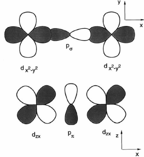
Figure 1: Examples of configurations for transition-metal $3d$ orbitals which are bridged by ligand $2p$ orbitals in transition metal oxides (after Ref. Ima98 ).

There are two crucial parameters which decide about the physical properties of a transition metal oxide, provided the $d-p$ hybridization elements are much smaller than the value of the on-site Coulomb interaction $U$. The latter parameter has to be compared with the splitting between the $3d$ and $2p$ orbitals, given by the so-called charge-transfer energy, $\Delta=|\varepsilon_{p}-\varepsilon_{d}|$, where $\varepsilon_{d}$ and $\varepsilon_{p}$ are the energies of an electron (hole) in these states, respectively. These systems are called Mott-Hubbard insulators (MHI) when $U<\Delta$, and it is in this limit that the Hubbard model would apply directly for the description of a metal-insulator transition. In the opposite case, one deals instead with charge-transfer insulators, as introduced by Zaanen, Sawatzky and Allen fifteen years ago Zaa85 ; Zaa90 . Both classes of correlated (in contrast to band) insulators have quite different spectral properties, but in the strongly correlated regime the charge-transfer insulators resemble MHI, with a charge-transfer energy $\Delta$ playing a role of the effective $U$ Mei93 .

In reality, however, many oxides are found close to the above qualitative boarder line between Mott-Hubbard and charge-transfer systems (Fig. 2), and one might expect that the only relevant description has to be based on the charge-transfer models which include explicitly both $d$ and $p$ orbitals. Nevertheless, a reduction of such models to the effective simpler Hamiltonians dealing only with correlated $d$-like orbitals is possible, and examples of such mapping procedure have been discussed in the literature Zha88 ; Fei96 ; Fei96a ; Fei96b . Unfortunately, there is no general method which works in every case, but the principle of the mapping procedure is clear, at least in perturbation theory. We will follow this idea in the present paper and concentrate ourselves on such simpler models which describe interactions between $3d$ electrons, determined by the effective hopping between transition metal ions which follows from intermediate processes involving charge-transfer excitations at the $2p$ oxygen orbitals Zaa88 . It will be clear from what follows that while this simplification is allowed, there is in general no way to reduce these models any further to those of nondegenerate $d$ orbitals, at least not for the oxides with a single electron or hole occupying (almost) degenerate $e_{g}$ orbitals.

We concentrate ourselves on a class of insulating strongly correlated transition metal compounds, where the crystal field leaves the $3d$ orbitals of $e_{g}$ symmetry explicitly degenerate and thus the type of occupied orbitals is not known a priori, while the effective magnetic interactions between the spins of neighboring transition metal ions are determined by orbitals which are occupied in the ground state Geh75 ; Kug82 ; Zaa93 ; Kho97 . The most interesting situation occurs when $e_{g}$ orbitals are partly occupied, which results in rather strong magnetic interactions, accompanied by strong Jahn-Teller (JT) effect. Typical examples of such ions are: Cu²⁺ ($d^{9}$ configuration, one hole in $e_{g}$-orbitals) Kug73 , low-spin Ni³⁺ ($d^{7}$ configuration, one electron in $e_{g}$-orbitals) Gar92 ; Med97 ; Rod98 , as well as Mn³⁺ Ram97 and Cr²⁺ ions (high-spin $d^{4}$ configuration with one $e_{g}$ electron). The situation encountered for $d^{9}$ (or $d^{7}$) transition metal ions is simpler, as the $t_{2g}$ orbitals are filled. The effective interactions may then be derived by considering only $e_{g}$ orbital degrees of freedom and spins $s=1/2$ at every site, and were first considered by Kugel and Khomskii more than two decades ago Kug73 . In the case of $d^{4}$ configuration one needs instead to consider larger spins $S=2$ which interact with each other, due to virtual excitation processes which involve either $e_{g}$ or $t_{2g}$ electrons Fei99 . Finally, the early transition-metal compounds with $d^{1}$ or $d^{2}$ ions give also some interesting examples of degenerate $t_{2g}$ orbitals Cas78 ; Bao97 ; Bao97a ; Pen97 ; Ezh99 ; Kei00 . In general, the magnetic superexchange and the coupling to the lattice are weaker in such cases due to a weaker hybridization between $3d$ and $2p$ orbitals (Fig. 1). Moreover, this problem is somewhat different due to the symmetry of the orbitals involved, and we will not discuss it here.

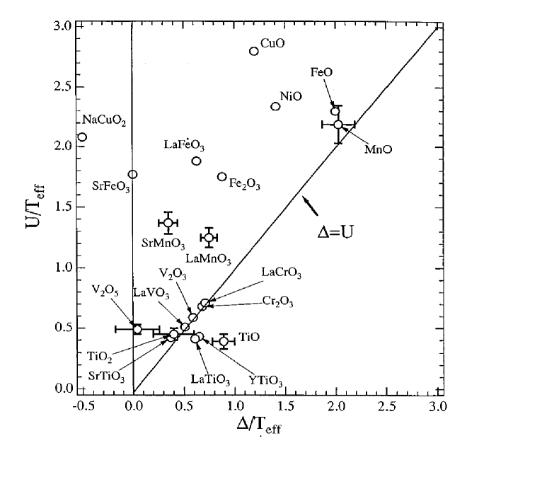
Figure 2: Zaanen-Sawatzky-Allen phase diagram for $3d$ transition metal oxides (after Ref. Boc96 ).

The collective behavior of $e_{g}$ electrons follows from their interactions. The models of interacting electrons in degenerate $3d$ states are usually limited to the leading on-site part of electron-electron interaction given by the Coulomb and exchange elements, $U$ and $J_{H}$, respectively. The model Hamiltonian which includes these interactions is of the form,

$$H_{int} =(U+2J_{H})\sum_{i\alpha}n_{i\alpha\uparrow}n_{i\alpha\downarrow}+(U-J_{H})\sum_{i,\alpha<\beta,\sigma}n_{i\alpha\sigma}n_{i\beta\sigma}+U\sum_{i,\alpha<\beta,\sigma}n_{i\alpha\sigma}n_{i\beta\bar{\sigma}}$$ (1)

$$-J_{H}\sum_{i,\alpha<\beta,\sigma}d^{\dagger}_{i\alpha\sigma}d_{i\alpha\bar{\sigma}}d^{\dagger}_{i\beta\bar{\sigma}}d_{i\beta\sigma}+J_{H}\sum_{i,\alpha<\beta}(d^{\dagger}_{i\alpha\uparrow}d^{\dagger}_{i\alpha\downarrow}d_{i\beta\downarrow}d_{i\beta\uparrow}+d^{\dagger}_{i\beta\uparrow}d^{\dagger}_{i\beta\downarrow}d_{i\alpha\downarrow}d_{i\alpha\uparrow}),$$

where summations over $\alpha<\beta$ guarantee that every pair of different states interacts only once, and we neglected the anisotropy of the interorbital interactions. It is important to realize that precisely for this reason the multiplet structure of transition metal ions Gri71 cannot be characterized by two quantities such as $U$ and $J_{H}$, but one needs instead three independent parameters, usually chosen as Racah parameters $A$, $B$, and $C$. The commonly used relation between these parameters and the Slater parameters $F_{0}$, $F_{2}$, and $F_{4}$ are given in Table II of Ref. Ima98 . We also emphasize that the last term which describes the hopping of double occupancies between different orbitals has the same amplitude as the spin exchange and is $\propto J_{H}$. Such terms are frequently neglected in the Hubbard-like models which thus cannot reproduce the correct multiplet structure and give uncontrolled errors when superexchange is derived from them.

Early applications of the model Hamiltonian (1) were devoted to the understanding of magnetic states of transition metals Ful91 ; Faz99 ; Ole83 ; Ole84a ; Ole84b . More recently, the Hamiltonian (1) has been used to improve the local density approximation (LDA) scheme for determining the electronic structure of correlated transition metal oxides by including the electron-electron interactions in the Hartree-Fock (HF) approximation which gives the so-called LDA+U method Ani91 . If the electron-electron interactions $U$ and $J_{H}$ are treated in the HF approximation, they generate local potentials which act on different local states $|i\alpha\sigma\rangle$, and allow thus for the ground states with anisotropic distributions of charge and magnetization over five $d$ orbitals. Such corrections improve the gap values in Mott-Hubbard and charge-transfer insulators, and become particularly important in the cuprates and manganites with partial filling of $e_{g}$ orbitals.

The consequences of local potentials which follow from the Coulomb and exchange terms in Eq. (1) are well seen on the example of KCuF₃, one of the compounds which exhibits the degeneracy of $e_{g}$ orbitals. We start out with the observation that according to LDA KCuF₃ would be an undistorted perovskite, as the energy increases if the lattice distortion is made (see Sec. III.C). The reason is that the band structure of KCuF₃ determined by LDA would give a band metal with a Fermi-surface which is not susceptible to a band JT instability. LDA+U yields instead a drastically different picture: it allows both the orbitals and the spins to polarize which results in an energy gain of order of the band gap, i.e., of the order of 1 eV and reproduces the observed orbital ordering Lie95 . The orbital- and spin polarization is nearly complete and the situation is close to the strong-coupling limit underlying the spin-orbital model of Sec. III.A.

Observed orbital ordering could also be obtained in manganites using the LDA+U approach Ani97 . As a remarkable success of this method, the orbital ordering which corresponds to the so-called CE phase with the orbital ordering accompanied by the charge ordering was obtained for Pr_1/2Ca_1/2MnO₃ Ani97 . In the undoped PrMnO₃ one finds that orbitals alternate between two sublattices in $(a,b)$ planes, as also expected following more qualitative arguments Kho97 , allowing thus for the ferromagnetic (FM) coupling between spins within the $(a,b)$ planes. In contrast, the orbitals almost repeat themselves along the $c$-axis, suggesting that the effective magnetic interactions should be AF. However, when the superexchange constants are determined using the band structure calculations Sol96 , they do not agree with the experimental data Hir96 ; Hir96a . Not only the FM exchange constants are larger by a factor close to four, but even the sign of the AF superexchange along the $c$-axis cannot be reproduced. Contrary to the suggestions made Sol96 , this result cannot be corrected by effective interactions between further neighbors, as the crystal structure and the momentum dependence of the spin-waves in LaMnO₃ indicate that only nearest neighbor interactions should contribute in the effective spin model Hir96 ; Hir96a , and represents one of the spectacular examples how the electronic structure calculations fail in strongly correlated systems. Therefore, it is necessary to study the effective models which describe the low-energy sector of excited states and treat more accurately the strong electron correlations, as presented in this article.

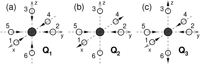
Figure 3: Different local modes for an MnO₆ octahedron: (a) breathing mode $Q_{1}$, (b) JT mode active in $(a,b)$ planes, and (c) JT tetragonal distortion $Q_{3}$. Filled and empty circles show Mn and O ions, respectively.

It is impossible to discuss the magnetic and orbital states of cuprates and manganites without paying attention to the lattice distortions. When the cubic crystal distorts, the energies of $e_{g}$ orbitals change due to the coupling to the lattice. Depending on the type of distortion, the energy of one or the other $e_{g}$ orbital will be lower. Therefore, particular lattice distortions alone might stabilize orbital ordering. In spite of some other views presented in the literature, we shall argue below that this is not the case for the cuprates, and the orbital ordering observed in KCuF₃ follows from the electronic interactions between strongly correlated electrons. We shall discuss this problem in particular for manganites (in Sec. V), where we argue that the electronic interactions alone determine the observed type of magnetic ordering, which is however additionally stabilized by the orbital interactions which follow from the JT effect Fei99 .

Let us recall first the single-ion (noncooperative) JT effect. It was realized long ago by Kanamori that local JT effect leads to the symmetry lowering for Cu²⁺ and Mn³⁺ ions with a single hole (electron) at octahedral sites Kan60 . He considered a single-site problem of an ion surrounded by six neighbors which may be distorted from their initial symmetric positions which satisfy the octahedral symmetry (see Fig. 3). The normal modes may be written as follows:

$$Q_{1} = \frac{1}{\sqrt{3}}(x_{1}-x_{4}+y_{2}-y_{5}+z_{3}-z_{6}),$$ (2)

$$Q_{2} = \frac{1}{\sqrt{2}}(x_{1}-x_{4}-y_{2}+y_{5}),$$ (3)

$$Q_{3} = \frac{1}{\sqrt{6}}(2z_{3}-2z_{6}-x_{1}+x_{4}-y_{2}+y_{5}),$$ (4)

where $x_{i}$, $y_{i}$ and $z_{i}$ are the coordinates of atom $i$. In contrast to the breathing mode $Q_{1}$, where all the neighbors move towards/away from the central site and the $e_{g}$ orbitals do not split, the other two normal modes ($Q_{2}$ and $Q_{3}$) remove orbital degeneracy and favor the occupancy of either $|x\rangle\equiv|x^{2}-y^{2}\rangle$ or $|z\rangle\equiv|3z^{2}-r^{2}\rangle$ orbital.

Following Kanamori Kan60 , we write the effective Hamiltonian in the form,

$$H_{JT} = H_{0}+H_{1}+H_{2},$$ (5)

$$H_{0} = \beta\lambda\sum_{i}Q_{1i},$$ (6)

$$H_{1} = \lambda\sqrt{C}\sum_{i\alpha\beta\sigma\sigma^{\prime}}c_{i\alpha\sigma}^{\dagger}(Q_{2i}\sigma_{i}^{x}+Q_{3i}\sigma_{i}^{z})_{\alpha\beta}c_{i\beta\sigma^{\prime}},$$ (7)

$$H_{2} = \frac{1}{2}C\sum_{i}(Q_{2i}^{2}+Q_{3i}^{2}),$$ (8)

where $c_{i\alpha\sigma}^{\dagger}$ is a creation operator for an $e_{g}$ electron in orbital $\alpha$ with spin $\sigma$, $\sigma_{i}^{x}$ and $\sigma_{i}^{z}$ are the Pauli matrices, and $\lambda$ and $\beta$ are the parameters which depend on the system. The ions at different sites are independent and one may solve just a single-site problem, assuming an ansatz for the orbital state,

$$|i\theta\sigma\rangle=\cos\theta|iz\sigma\rangle+\sin\theta|ix\sigma\rangle.$$ (9)

Using the uniform angle $\theta_{i}=\theta$, the classical distortions and the coordinates and the orbital state are given as follows:

$$Q_{2i}^{0} = \frac{\lambda}{\sqrt{C}}\sin 2\theta,\hskip 28.45274ptQ_{3i}^{0}=\frac{\lambda}{\sqrt{C}}\cos 2\theta,$$ (10)

$$\langle\sigma_{i}^{z}\rangle = \cos 2\theta,\hskip 39.83368pt\langle\sigma_{i}^{x}\rangle=\sin 2\theta.$$ (11)

As easily recognized from Eqs. (10) and (11), the orbital state follows the lattice distortions and one finds the energy minimum given by $-\lambda^{2}/2$, showing that the lowest state cannot be determined uniquely. The situation changes when anharmonic terms are included which lead to the energy contribution of the form,

$$H_{A}=-A\sum_{i}\cos 6\theta_{i},$$ (12)

with $A>0$. This term favors directional orbitals, and tetragonal distortions with the elongated tetragonal axis is the most stable structure. One finds identical energy for three different distortions, corresponding to $3z^{2}-r^{2}$ orbital at $\theta=0$, and to $3x^{2}-r^{2}$ ($3y^{2}-r^{2}$) orbital at $\theta=\pm\pi/3$, respectively.

The above energy contributions occur for the sites occupied by a single $e_{g}$ electron, as for instance at Mn³⁺ ions. Important deformations of the lattice occur as well around Mn⁴⁺ ions, when the $e_{g}$ electron is absent. In this case the breathing mode $Q_{1}$ becomes active, and the respective energy contribution takes the form,

$$H_{hole}=\beta\lambda\sum_{i}(1-n_{i})Q_{1i},$$ (13)

and typically $\beta\gg 1$.

Although the tendency towards directional orbitals might be considered to be generic for the present systems, such states cannot occur independently of each other in a crystal, as the lattice distortions are correlated. Therefore, a more realistic description requires a coupling between the oxygen distortions realized around different manganese sites. We discuss this problem on the example of LaMnO₃, which has been studied in more detail only recently Mil96 ; Rod96 . If oxygens around a given Mn³⁺ ion are distorted, there are also distortions of common oxygen atoms around the neighboring Mn³⁺ ions, and in this way the orbital angles are coupled to each other. This is called cooperative JT effect, in contrast to the noncooperative one Kan60 which concerns single sites. The total energy which follows from the coupling to the lattice was derived by Millis Mil96 :

$$H_{lat} = -|E_{0}|\sum_{i}[n_{i}^{2}+\beta^{2}(1-n_{i})^{2}+A\cos 6\theta_{i}]$$ (14)

$$+\kappa\sum_{\langle ij\rangle}n_{i}n_{j}\cos 2(\theta_{i}+\psi_{\alpha})\cos 2(\theta_{j}+\psi_{\alpha})$$

$$+2\beta\kappa\sum_{\langle ij\rangle}(1-n_{i})n_{j}\cos 2(\theta_{j}+\psi_{\alpha})+\beta^{2}\kappa\sum_{\langle ij\rangle}(1-n_{i})(1-n_{j}).$$

It includes the on-site terms, and the intersite couplings along the bonds, making the JT effect cooperative. A particular tendency for occupying the orbitals of a given type is expressed by the terms $\cos 2(\theta_{i}+\psi_{\alpha})$, with the angle $\psi_{\alpha}$ depending on the bond direction as follows: $\psi_{c}=0$, $\psi_{a}=-\pi/3$, and $\psi_{b}=\pi/3$, for the bonds $\langle ij\rangle$ along the $c$, $a$, and $b$-axis, respectively. The coupling constants $E_{0}$ and $\kappa$ depend on the coefficient $\lambda$ introduced in Eq. (7) and are functions of the respective force constants which describe the coupling between the manganese and oxygens ions, and between the pairs of oxygen ions, respectively. For the purpose of these lectures we will treat them as phenomenological parameters, but an interested reader may find explicit expressions and more technical details in Ref. Mil96 .

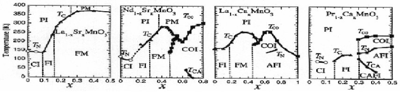
Figure 4: Phase diagrams of A_1-xB_xMnO₃ compounds (after Ref. Ima98 ). Various ordered phases are labeled as follows: FI (PI) – ferromagnetic (paramagnetic) insulator, FM (PM) – ferromagnetic (paramagnetic) metal, CI – spin-canted insulating, COI – charge-ordered insulating, AFI – antiferromagnetic insulating, CAFI – canted antiferromagnetic insulating.

Recent extensive research on the CMR manganites has generated a huge number of papers in the scientific literature. The interest is motivated by very spectacular experimental properties, with typically several magnetic phases stable in different doping regimes, most of them insulating, but one metallic FM phase Ima98 ; Ram97 . With increasing temperature a transition from the FM metallic phase occurs either to a paramagnetic metal, or at lower doping to a paramagnetic insulator. In the latter case a large change of the resistivity accompanies the phase transition, and the transition temperature is strongly modified by the external magnetic field, giving rise to the phenomenon of CMR Jin94 . Examples of magnetic phase diagrams for representative distorted perovskites R_1-xA_xMnO₃ are shown in Fig. 4. The FM metallic phase is found in first three compounds, while in Pr_1-xCa_xMnO₃ all magnetic phases are insulating. As the average ionic radius of the perovskite A site increases from (La,Sr) to (Pr,Ca) through (Nd,Sr) or (La,Ca), orthorhombic distortion of the GdFeO₃ type Ima98 increases, resulting in the decrease of the decrease of the one-electron bandwidth $W$. When the bandwidth gets reduced, the balance between the double-exchange (DE) Zen51 ; And55 and other interactions changes and such instabilities as JT type distortions, charge and/or orbital ordering may occur. Moreover, the AF superexchange may play an important role and stabilize the AF order in a broader doping regime.

In order to understand the phase diagrams of manganites, one needs to consider four different kinds of degrees of freedom: charge, spin, orbital, and lattice. Therefore, the models which treat doped manganites in a realistic way are rather sophisticated. A somewhat simpler situation occurs in the undoped LaMnO₃ as the charge fluctuations are suppressed by large on-site Coulomb interactions and one may study effective magnetic and orbital interactions, as we present in Sec. V.A. This problem may be also approached in a phenomenological way by postulating model Hamiltonians which contain such essential terms as the Hund’s rule exchange interaction between $e_{g}$ and $t_{2g}$ electrons, the AF interactions between the $t_{2g}$ core spins, and the coupling to the lattice. As an example, we present the Hamiltonian of the degenerate Kondo lattice with the coupling to local distortions of MnO₆ octahedra Hot99 ,

$$H = \sum_{ij\alpha\beta\sigma}t_{\alpha\beta}c_{i\alpha\sigma}^{\dagger}c_{j\beta\sigma}-J_{H}\sum_{i\alpha\sigma\sigma^{\prime}}{\vec{S}}_{i}\cdot c_{i\alpha\sigma}^{\dagger}{\vec{\sigma}}_{\sigma\sigma^{\prime}}c_{i\beta\sigma}+J^{\prime}\sum_{\langle ij\rangle}{\vec{S}}_{i}\cdot{\vec{S}}_{j}$$ (15)

$$+ \lambda\sum_{i\alpha\beta\sigma}c_{i\alpha\sigma}^{\dagger}(Q_{1i}\sigma^{0}_{i}+Q_{2i}\sigma^{x}_{i}+Q_{3i}\sigma^{z}_{i})_{\alpha\beta}c_{i\beta\sigma}+\frac{1}{2}\sum_{i}(\beta Q_{1i}^{2}+Q_{2i}^{2}+Q_{3i}^{2}),$$

where $c_{i\alpha\sigma}^{\dagger}$ is the creation operator of an $e_{g}$ electron with spin $\sigma$ in the $d_{x^{2}-y^{2}}$ ($d_{3z^{2}-r^{2}}$) orbital at site $i$. The hopping elements $t^{\alpha\beta}_{ij}$ between nearest neighbors follow from the Slater-Koster rules Sla54 . ${\vec{S}}_{i}$ is the localized spin of $t_{2g}$ electrons, and $\sigma^{x}_{i}$ and $\sigma^{z}_{i}$ are Pauli matrices. $\lambda$ stands for the dimensionless electron-phonon coupling constant. Different distortions $Q_{1i}$, $Q_{2i}$, and $Q_{3i}$ are the breathing mode and two JT modes shown in Fig. 3. Hotta et al. Hot99 took into account the cooperative nature of the JT phonons by introducing the coupling between the neighboring Mn ions in the normal coordinates for distortions of MnO₆ octahedra Mil96 ; All99 . The important parameter is the ratio of the vibrational energies for manganite breathing ($\omega_{b}$) and JT ($\omega_{\rm JT}$) modes, $\beta=(\omega_{b}/\omega_{\rm JT})^{2}$.

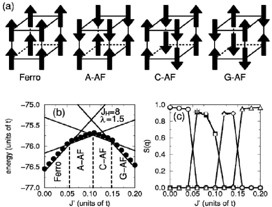
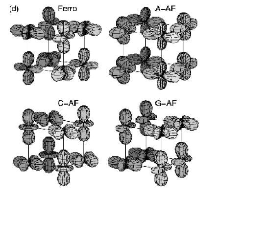
Figure 5: Types of magnetic order (a) and orbital order (d) in perovskite structures: Ferro, A-AF, C-AF, and G-AF, as obtained in MC simulations by Hotta et al. Hot99 using a model of $e_{g}$ electrons coupled to the core $t_{2g}$ spins and to JT lattice distortions (15). Quantitative results obtained as functions of the AF coupling $J^{\prime}$ between $t_{2g}$ spins for $J_{H}=8$ and $\lambda=1.5$ are shown by two middle panels: (b) the total energy for a $2\times 2\times 2$ lattice; (c) the spin-spin structure factor $S({\vec{q}})$ obtained for $4\times 4\times 2$ (solid symbols) and $4\times 4\times 4$ (open symbols) clusters. The circles, squares, diamonds, and triangles indicate $S({\vec{q}})$ for ${\vec{q}}=(0,0,0)$, ${\vec{q}}=(\pi,0,0)$, ${\vec{q}}=(\pi,\pi,0)$, and ${\vec{q}}=(\pi,\pi,\pi)$, respectively.

The calculations performed by the relaxation technique and by Monte-Carlo Yun98 for finite 3D clusters are summarized in Fig. 5. Depending on the parameters, four different magnetic phases are found [Fig. 5(a)]: FM phase (Ferro), so-called A-AF phase with staggered FM planes, C-AF phase with staggered FM chains, and, finally, the G-AF phase which is the 3D Néel order. They are identified by investigating the magnetic structure factor $S({\vec{q}})=\frac{1}{N}\sum_{ij}\exp[i{\vec{q}}({\vec{R}}_{i}-{\vec{R}}_{j})\langle{\vec{S}}_{i}{\vec{S}}_{j}\rangle$ [Fig. 5(c)]. It is straightforward to understand that the ground state is FM at $J^{\prime}=0$. In this case the lowest energy gain may be obtained from the combination of the kinetic energy of $e_{g}$ electrons with the local Hund’s rule $\propto J_{H}$. Increasing $J^{\prime}$ increases the tendency towards the AF order and leads finally to the G-AF phase in the range of large $J^{\prime}/t>0.15$ [Fig. 5(b)].

Hotta et al. Hot99 found that various magnetic orderings are accompanied by the orbital orderings shown in Fig. 5(d)]. The shape of the occupied orbital arrangment is not easy to understand, however. It follows from the cooperative JT effect and expresses a compromise between the orbital and magnetic energies. The overall picture might seem appealing, but it is questionable whether the JT effect is the dominating mechanism that determines the magnetic and orbital ordering in manganites and related compounds which are known to be primarily MHI Ima98 , i.e., the on-site Coulomb interaction $U$ is the largest parameter, typically $5<U<10$ eV, which dominates the hybridization. Although it has been argued that the large Coulomb interaction will not change the main results shown in Fig. 5 Hot99 , we do not think this conclusion is allowed. In fact, in the absence of large Coulomb interaction $U$ the magnetic interactions are dominated by DE And55 and the system is FM at $J^{\prime}=0$ as new effective interactions arise in the presence of large $U$, and they easily might change the delicate balance between different magnetic and orbital ordered phases. We shall discuss the problem of magnetic and orbital ordering in detail in Secs. III and V and show that the electronic interactions alone give a dominating contribution to magnetic interactions.

Magnetism in transition metals and in their compounds is known to be due to intraatomic Coulomb interaction Sla36 . The simplest model which takes into account the Coulomb interaction is that due to Hubbard (see Sec. II.A). It describes electrons in a narrow and nondegenerate tight-binding band and allows for repulsion $U$ between electrons only when they are at the same site. This model has been studied intensively since Hubbard proposed it, especially in connection to the occurrence of magnetism Faz99 . Anderson has shown in 1959 And59 that the Hubbard Hamiltonian is equivalent to a Heisenberg Hamiltonian with an AF superexchange interaction given in terms of the hopping amplitude and the Coulomb interaction, if $U$ is large. Indeed, for two neighboring ions an extra delocalization process $d^{1}_{i}d^{1}_{j}\rightarrow d^{0}_{i}d^{2}_{j}$ is only possible for antiparallel arrangment of neighboring spins, decreasing the energy and favoring this configuration (Fig. 6). Therefore, if each ion has only one nondegenerate orbital, the superexchange is AF, as explained in Sec. II.A.

The question of whether the AF correlations might evolve by changing the electron concentration into ferromagnetism is still controversial. A rigorous proof of Nagaoka Nag66 of the existence of ferromagnetism applies only in a very special case – in the limit of infinite Coulomb repulsion $U$ when one hole or one extra electron is added to the half-filled band ($n=1$), in a lattice of particular symmetry. However, the occurrence of ferromagnetism comes in a more natural way if one takes into account the orbital degeneracy as Van Vleck has emphasized Vlec53 . In the case of two-fold orbital degeneracy, applying similar arguments as those used by Anderson And59 , one ends up with a richer structure of effective interactions when the processes $d^{1}_{i}d^{1}_{j}\rightarrow d^{0}_{i}d^{2}_{j}$ are analyzed. For the occupancy of $n=1$ electron per atom one finds four possible situations as depicted in Fig. 6: (a) same orbital – same spin, (b) same orbital – different spin, (c) different orbital – same spin, (d) different orbital – different spin. This problem has been studied already in the seventies, but mostly starting from simplified model Hamiltonians Cyr75 ; Cyr75a ; Cyr75b ; Spa80 . In order to study the qualitative effects, the simplest case with only diagonal hopping and equal intra- and interorbital Coulomb elements $U$ in Eq. (1) has been usually assumed.

As a qualitative new effect due to the Hund’s rule exchange $J_{H}>0$, ferromagnetic superexchange becomes possible, if the excitation involves the high-spin state with two parallel electrons [Fig. 6(c)]. Although the processes which contribute to the superexchange for nondegenerate orbitals [Fig. 6(b)] are also present, and there are more AF terms, the FM term has the largest coefficient due to the structure of Coulomb interactions (1). Therefore, one might expect that under certain conditions such terms could promote ferromagnetism. While this is not easy and happens only for rather extreme parameters in the doubly degenerate Hubbard model with isotropic but diagonal hopping elements Cyr75 ; Cyr75a ; Cyr75b , it has been recognized in these early works that the orbital ordering may accompany the magnetic ordering, and orbital superlattice favors the appearance of magnetism at zero temperature. Indeed, the onset of magnetic long-range order (LRO) is obtained for such values of parameters that the usual Stoner criterion is not yet fulfilled. Furthermore, the studies at finite temperature revealed that the orbital order is more stable than the magnetic one. Therefore, two phase transitions are expected in general: at the lower temperature the ferromagnetism disappears and, at the higher one, the orbital order Cyr75 ; Cyr75a ; Cyr75b .

In order to understand the behavior of CMR manganites, it is necessary to include the orbital degrees of freedom for partly occupied $e_{g}$ orbitals. The motivation comes both from theory and experiment. For quite long time it was believed that the FM state in manganites can be understood by the DE model Zen51 ; And55 . In fact, it provides not more than a qualitative explanation why the doped manganites should have a regime of FM metallic state (Fig. 4). However, if one calculates the Curie temperature $T_{C}$ using the DE model the values are overestimated by a factor of the order of five Mil95 . Also the experimental dependence of the resistivity in the metallic phase Uru95 cannot be reproduced within the DE model Mil95 . Finally, in a FM metal one expects a large Drude peak and no incoherent part in the optical conductivity. The experimental result is quite different – most of the intensity is incoherent at low temperatures, and only a small Drude peak appears which absorbs not more than 20 % of the total spectral weight Oki97 ; Oki95 . All these results demonstrate the importance of orbital degrees of freedom which should be treated on equal footing as the spins of $e_{g}$ electrons.

Figure 6: The various configurations of nearest neighbors for doubly-degenerate orbitals. The kinetic exchange is always AF in a nondegenerate model (b), while the processes which involve differently occupied orbitals on both sites may be either FM (c) or AF (d). $U$ and $J_{H}$ are the on-site Coulomb and Hund’s rule exchange interactions (after Ref. Kho97 ).

The orbital degeneracy leads therefore to a new type of models in the theory of magnetism: spin-orbital models. They act in the extended space and describe the (super)exchange interactions between spins, between orbitals, and simultaneous spin-and-orbital couplings. In order to address realistic situations encountered in cuprates and manganites, such models cannot rely on the degenerate Hubbard model Cyr75 ; Cyr75a ; Cyr75b , but have to include the anisotropy in the hopping elements Sla54 , nonconservation of the orbital quantum number, and realistic energetic structure of the excited states Gri71 . Once such models are derived, as we present in Secs. III and V, their phase diagrams may be studied using the mean-field (MF) approximationFei99 ; Fei97 ; Ole00 . It turns out that their phase diagrams show an unusual competitions between classical (magnetic and orbital) ordering of different type, in particular close to the degeneracy of $e_{g}$ orbitals. Therefore, two interesting questions occur for such orbitally degenerate MHI: (i) Which classical states with magnetic LRO do exist in the neighborhood of orbital degeneracy? (ii) Are those forms of classical order always stable against quantum (Gaussian) fluctuations? We will show that the orbitally degenerate MHI represent a class of systems in which spin disorder occurs due to frustration of spin and orbital superexchange couplings. This frustration mechanism is different from that which operates in quantum antiferromagnets, and suppresses the magnetic LRO in the ground state even in three dimensions.

We organized the remaining chapters of this article as follows. In order to clarify the basic magnetic interactions in strongly correlated oxides, we start with the superexchange and DE in Sec. II. Next we introduce and analyze on the classical level the simplest spin-orbital model for spins $S=1/2$ (Sec. III) which applies to cuprates, and present its collective modes. The model exhibits an interesting frustration of magnetic interactions, and the classical phases are destabilized by quantum fluctuations (Sec. IV). Therefore, we discuss the problem of quantum disorder in low dimensional spin models and in an idealized spin-orbital model with SU(4) symmetry in one dimension. The physics of manganites is richer than that of cuprates close to the degeneracy of $e_{g}$ orbitals, and additional interactions between orbital variables occur due to the coupling to the lattice (Sec. V). The understanding of various phase transitions shown in Fig. 4 remains an outstanding problem which requires to study simultaneously the coupling to the lattice responsible for the insulating behavior of doped systems, and the DE model at orbital degeneracy. This latter problem is very actual and was addressed for the first time only last year Bri99 (Sec. VI). The spin and orbital interactions lead in general to new type of effective $t$-$J$ models Zaa93 , and we analyze spin-waves in FM phase and give an example of the hole which dresses by orbital excitations and compare this situation with the hole motion in the $t$-$J$ model (Sec. VII). Among many open questions for doped manganites, we selected a few such as the CE-phase, stripes, orbital ordering and phase separation (Sec. VIII). In our opinion, they are crucial to understand the complexity of the experimental phase diagrams. We give a brief summary and our conclusions in Sec. IX.

II Magnetic interactions for nondegenerate orbitals

II.1 Superexchange and $t$-$J$ model

Before discussing the consequences of $e_{g}$ orbital degeneracy in cuprates and manganites, we review shortly the basic magnetic interactions in the models of nondegenerate orbitals – the superexchange and the DE. The main idea to derive the superexchange is the notion of the Mott-Hubbard insulator at $n=1$ in which the charge fluctuations are suppressed and the electrons localize, occupying the states of the lower Hubbard band. Therefore, part of degrees of freedom is integrated out and one may study an effective model which captures the essential features of the low-energy excitations.

Before deriving the effective superexchange model for degenerate orbitals, we analyze shortly the nondegenerate orbitals filled by one electron per atom  ($n$=1). This situation plays a fundamental role in strongly correlated systems and elucidates the general principle of introducing magnetic (and orbital) interactions in a Mott-Hubbard insulator by integrating out charge fluctuations and reducing the problem. The starting point is the Hubbard Hamiltonian,

$$H = H_{t}+H_{U},$$ (16)

$$H_{t} = -t\sum_{\langle ij\rangle\sigma}\left(c^{{\dagger}}_{i\sigma}c_{j\sigma}+H.c.\right),$$ (17)

$$H_{U} = U\sum_{i}n_{i\uparrow}n_{i\downarrow},$$ (18)

where $U$ and $t$ are standing for the on-site screened Coulomb repulsion, and for the hopping amplitude between nearest neighbors, respectively, and the summation runs over the bonds $\langle ij\rangle$ between nearest neighbors. Furthermore, the operator $c^{{\dagger}}_{i\sigma}$ creates an electron with spin $\sigma$ at site $i$, and $n_{i\sigma}=c^{{\dagger}}_{i\sigma}c_{i\sigma}$ is the electron density operator. Recall that the interaction term in the Hubbard model can be reexpressed in the following way:

$$H_{U}=-\frac{2}{3}U\sum_{i}\left(\vec{S}_{i}\right)^{2},$$ (19)

so that it forces the spin $\vec{S}_{i}$ to be maximal if $U$ becomes infinitely large, i.e., doubly occupied sites are forbidden. Only $\mid\uparrow\rangle$ and $\mid\downarrow\rangle$ states are kept in this large $U$ limit at half-filling. Taking the atomic limit ($t=0$), the interaction part of the Hamiltonian (16) has infinitely many ($2^{N}$, where $N$ is the number of sites) degenerate eigenstates, given by different spin configurations. In order to lift this large degeneracy we will keep the effects of fluctuations induced by the kinetic energy term to leading order in an expansion in $(t/U)$. As usually, this problem has to be solved in degenerate perturbation theory.

Suppose we begin with an arbitrary configuration which can be labeled by the local $z$th components of the spins $S_{i}^{z}$. In the expansion in powers of $(t/U)$, one includes contributions from intermediate states in which one site will become doubly occupied and, at the same time, the other site becomes empty Cha77 . The energy of the excited state is $U$ above that of the degenerate ground state manifold. The squared transition matrix element is $t^{2}$ and the combinatorial factor of two has to be included since this process can occur in two different ways. Hence we expect that the relevant parameter of the effective spin Hamiltonian should be $2t^{2}/U$. Also, the final state after the double occupancy dissociates has to be either the same as the initial state, or it may differ at most by a spin exchange. The candidate for the effective Hamiltonian is, of course, the quantum Heisenberg antiferromagnet Cha77 ; And59 ; Spa80 , since we know that the spin-spin interaction follows from a possibility of permuting the electrons on a lattice.

The formal derivation of the effective Heisenberg model can be performed in a few different equivalent ways: (i) by means of a canonical transformation Cha77 , (ii) with Schrieffer-Wolff procedure Sch66 , and (iii) with Brillouin-Wigner perturbation approach Baym74 . The first method is the most transparent to use away from the half-filling, where it leads to the $t$-$J$ model, known as a minimal model to describe the electronic states in high temperature superconductors Dag94 . We will not repeat here the details of the derivation of the $t$-$J$ model Cha77 as it belongs already to the textbook material Ful91 ; Faz99 . The common result of all these procedures at $n=1$ is the removal of degeneracy within the second order perturbation, and the effective Hamiltonian, given by the following expression:

$$\langle\phi|H_{eff}|\psi\rangle=-\langle\phi|H_{t}\frac{1-P_{0}}{H_{U}}H_{t}|\psi\rangle=-\sum_{n\neq\{0\}}\langle\phi|H_{t}|n\rangle\frac{1}{U}\langle n|H_{t}|\psi\rangle,$$ (20)

where $|\phi\rangle,|\psi\rangle$ denote states in the subspace without double occupancies, with a projection operator P₀. The states $|n\rangle$ are configurations with one doubly occupied site, and each term in the sum can be represented by a retraceable exchange path. Thereby we assume that $n\leq 1$; the case of $n>1$ may be treated by the same method after performing a particle-hole transformation. Since the total spin per two sites is conserved in the excitation process $\mid\uparrow\rangle_{i}\mid\downarrow\rangle_{j}\rightarrow|0\rangle_{i}\mid\uparrow\downarrow\rangle_{j}$, we can express the operators which connect the initial and final states of this transition by means of the projection operators for the singlet and for the triplet state on the bond $\langle ij\rangle$, respectively:

$$Q_{S}(i,j)=\left(-\vec{S_{i}}\cdot\vec{S_{j}}+\frac{1}{4}\right),\hskip 28.45274ptQ_{T}(i,j)=\left(\vec{S_{i}}\cdot\vec{S_{j}}+\frac{3}{4}\right).$$ (21)

The excitation energy associated to the process $\mid\uparrow\rangle_{i}\mid\downarrow\rangle_{j}\rightarrow|0\rangle_{i}\mid\uparrow\downarrow\rangle_{j}$ which creates a singlet at site $j$ is $\varepsilon_{S}=U$, (if we start from a triplet configuration, virtual processes are blocked due to the Pauli principle). Taking into account that the double occupancy may be created either at site $i$ or at site $j$, the effective Hamiltonian can be expressed in the following way,

$$H_{eff}=-\frac{4t^{2}}{U}\sum_{\langle ij\rangle}Q_{S}(i,j)=J\sum_{\langle ij\rangle}\left(\vec{S_{i}}\cdot\vec{S_{j}}-\frac{1}{4}\right).$$ (22)

Thus, one finds the AF Heisenberg model with the superexchange constant
$J$=$4t^{2}/U$.

II.2 Kondo lattice model – double exchange

The early theoretical studies of manganites were concentrated on the models introduced in order to understand the FM phase which occurs in the doped materials. The basic understanding of the tendency towards FM order follows from the so-called double exchange model Zen51 ; And55 – it explains that electrons in a partially filled band maximize their kinetic energy when their spins are aligned with the localized spins which order ferromagnetically. In fact, this phenomenon is quite reminiscent of the Nagaoka state in the Hubbard modelNag66 . However, in spite of this qualitative explanation of the existence of ferromagnetism, several features of the experimental phase diagrams of manganites remain unclear especially at low temperature, where one has to go beyond the DE model. In order to understand the reasons of its shortcomings, let us present briefly the main consequences of the DE model.

The Kondo lattice Hamiltonian with ferromagnetic spin-fermion coupling can be defined as follows,

$$H=-t\sum_{\langle{ij}\rangle\sigma}(c^{\dagger}_{i\sigma}c_{j\sigma}+H.c.)-J_{H}\sum_{i\alpha\beta}{\vec{S}}_{\bf i}\cdot{c^{\dagger}_{i\alpha}{\vec{\sigma}}_{\alpha\beta}c_{i\beta}},$$ (23)

where $c_{i\sigma}^{\dagger}$ is a creation operator for an electron at site $i$ with spin $\sigma$, and ${\vec{S}}_{i}$ is the total spin of the $t_{2g}$ electrons $S=3/2$, assumed to be localized. The first term describes the kinetic energy of electrons in a nondegenerate band due to the electron transfer between nearest-neighbor Mn-ions, $J_{H}>0$ is the FM Hund’s coupling between the itinerant electron and the $t_{2g}$ core spin ($S=3/2$). The average electronic density of $e_{g}$ electrons, denoted by $n=\langle n_{i}\rangle$, is adjusted using a chemical potential $\mu$.

Let us consider a bond in the perovskite structure formed by two Mn atoms with an oxygen atom in between. In the ionic configuration the $2p$ shell of the O^2- ion is completely filled. In order to treat the problem semiclassically And55 , we assume that the Mn ions have rather large spins $S_{1}$ and $S_{2}$, so that one could assign to them definite directions in space, and a definite angle relative to each other. If an itinerant $e_{g}$ electron is on the site $i=1$, it has two states, of energies $E_{1}=\pm JS$, if the electron spin is parallel and antiparallel to the spin ${\vec{S}}_{1}$, respectively. On atom $i=2$ it also has similar two states, but defined with respect to the direction of spin ${\vec{S}}_{2}$. As the electron spin direction is conserved in the hopping process, the final state has to be projected on the new local axis. This is equivalent to rotating the transfer matrix between these two sites in such a way that its elements refer correctly to the projected spin components in the rotated basis.

Let us label the two electronic spin functions referring to the direction of ${\vec{S}}_{1}$ by $\alpha$ and $\beta$, and those referring to ${\vec{S}}_{2}$ by $\alpha^{\prime}$ and $\beta^{\prime}$. The energies of the eigenstates on atom $i=1$ are:

$$E(d_{1}\alpha)=-J_{H}S,\hskip 28.45274ptE(d_{1}\beta)=J_{H}(S+1),$$ (24)

for FM coupling $J_{H}>0$. The energies of the eigenstates on atom $i=2$ are given by similar expressions:

$$E(d_{2}\alpha^{\prime})=-J_{H}S,\hskip 28.45274ptE(d_{2}\beta^{\prime})=J_{H}(S+1).$$ (25)

Here $d_{1}$ and $d_{2}$ describe the spin function of an electron localized at atom 1 and atom 2, respectively.

The transformation which expresses $\alpha$ and $\beta$ in terms of $\alpha^{\prime}$ and $\beta^{\prime}$ is of the form,

$$\alpha = \cos(\theta/2)\alpha^{\prime}+\sin(\theta/2)\beta^{\prime},$$ (26)

$$\beta = -\sin(\theta/2)\alpha^{\prime}+\cos(\theta/2)\beta^{\prime},$$ (27)

where $\theta$ is the angle between the spins $\overrightarrow{S_{1}}$ and $\overrightarrow{S_{2}}$. By considering the Hamiltonian (23) for two sites, one can write the secular equation which has the following four solutions And55 :

$$E=1/2J\pm\Big{(}[J(S+1/2)\pm t\cos(\theta/2)]^{2}+t^{2}\sin^{2}(\theta/2)\Big{)}^{1/2}.$$ (28)

The energies depend on the angle $\theta$ between both spins, and in the semiclassical case

$$\cos\left(\frac{\theta}{2}\right)=\frac{|\vec{S}_{1}+\vec{S}_{2}|}{2S}.$$ (29)

In the absence of any other interaction, the lowest energy is obtained for the aligned spins, at $\theta=0$.

The existence of phase separation and ferromagnetism in the ground state of the FM Kondo model can also be studied in the limit of $d=\infty$. The dynamical mean field theory (DMFT) Geo96 leads to a self-consistent equation which can be solved iteratively starting from a random spin configuration, and as a function of temperature and electron density three solutions have been found with AF, FM, and paramagnetic character. We refer an interested reader to Ref. Fur98 for more technical details.

The presence of ferromagnetism at finite doping and antiferromagnetism at half-filling are quite clear from Fig. 7. Close to half-filling and at low temperature, the density $n=\langle n_{i}\rangle$ was found to be discontinuous as a function of $\mu$, in excellent agreement with the results obtained by other numerical calculations. The phase separation observed in Fig. 7(a) occurs between AF and FM regions. However, we note that at higher temperature the phase separation occurs between hole-poor AF and hole-rich paramagnetic regions [Fig. 7(b)].

Figure 7: (a) Phase diagram in the $d=\infty$ limit working at $J_{H}/W=4.0$. The “PS(AF-PM)” region denotes phase separation (PS) between a hole-poor antiferromagnetic (AF) region, and a hole-rich paramagnetic (PM) region. The rest of the notation is standard; (b) Density $\langle n\rangle$ vs $\mu/W$ obtained in the $d=\infty$ limit, $J_{H}/W=4.0$, and $T/W=0.0003$. The discontinuity in the density is clear (after Ref. Fur98 ).

In order to illustrate the consequences of the DMFT treatment of the Kondo lattice (DE) model (23) we reproduce in Fig. 8 the density of states $A(\omega)$ obtained for the AF and FM phases at low temperature (for details of the calculation see Ref. Fur98 ). The critical value of the chemical potential where the AF and FM phases coexist is $\mu_{c}\simeq-1.40W$. In the both cases the density of states splits into upper and lower bands due to the large Hund’s coupling $J_{H}$. The band splitting in the FM phase is due to the half-metalicity of the system. The width of the upper and lower bands is wider for the FM phase, which causes a narrower gaped region centered at $\omega\simeq 0$.

Figure 8: Density of states in the $d=\infty$ limit corresponding to the AF (solid line) and FM (dotted line) solutions, found at $J_{H}/W=2.0$ and $T/W=0.005$ (after Ref. Fur98 ).

Following Furukawa Fur96 , we calculate the spin excitation spectrum of the DE model, and compare the results with recent data of the neutron inelastic scattering experiments. We use the spin-wave approximation in the ground state, which has been introduced by Kubo and Ohata Kub72 . Expanding the spin operators in terms of boson operators in the FM state,

$$S_{i}^{+}\simeq\sqrt{2S}a_{i},\hskip 28.45274ptS_{i}^{-}\simeq\sqrt{2S}a_{i}^{\dagger},\hskip 28.45274ptS_{i}^{z}=S-a_{i}^{+}a_{i},$$ (30)

the lowest-order effective Hamiltonian can be written as follows:

$$H = \sum_{\vec{k}}\left[(\varepsilon_{\vec{k}}-J_{H})c_{{\vec{k}}\uparrow}^{\dagger}c_{{\vec{k}}\uparrow}+(\varepsilon_{\vec{k}}+J_{H})c_{{\vec{k}}\downarrow}^{\dagger}c_{{\vec{k}}\downarrow}\right]$$ (31)

$$+ J_{H}\sqrt{\frac{2}{SN}}\sum_{{\vec{k}}{\vec{q}}}\left(a_{\vec{q}}^{\dagger}c_{{\vec{k}}\uparrow}^{\dagger}c_{{\vec{k}}+{\vec{q}},\downarrow}+a_{\vec{q}}c_{{\vec{k}}+{\vec{q}},\downarrow}^{\dagger}c_{{\vec{k}}\uparrow}\right)+\frac{J_{H}}{SN}\sum_{{\vec{k}}{\vec{q}}_{1}{\vec{q}}_{2},\sigma}\sigma a_{{\vec{q}}_{1}}^{\dagger}a_{{\vec{q}}_{2}}c_{{\vec{k}}-{\vec{q}}_{1}\sigma}^{\dagger}c_{{\vec{k}}-{\vec{q}}_{2}\sigma}.$$

The first line in Eq. (31) describes the electron band split by the exchange interaction with the core spins, while the second line stands for the coupling between the electrons and spin excitations (electron-magnon interaction).

Let us consider the lowest order terms of the $1/S$ expansion at $T=0$, assuming that $J_{H}$ is finite but sufficiently large to polarize completely the electronic band, i.e., $n_{\uparrow}=n$ and $n_{\downarrow}=0$, at $T=0$. The electron concentration is given by $n=1-x$. For a simple cubic 3D lattice with nearest-neighbor hopping $t$ one finds,

$$\varepsilon_{\vec{k}}=-2t\left(\cos k_{x}+\cos k_{y}+\cos k_{z}\right)=-6t\gamma_{\vec{k}},$$ (32)

where $\gamma_{\vec{k}}=\frac{1}{z}\sum_{\vec{\delta}}\exp(i{\vec{k}}\cdot{\vec{\delta}})$. For perovskite manganites, estimates of the electron bandwidth and the on-site Hund’s coupling being a few eV has been made by the first-principle calculations. However, one might consider that $t$ and $J_{H}$ in the DE model are effective parameters which could be strongly renormalized from the bare values due to other interactions present in the real systems. Such effective parameters could be determined from a comparison with experiments.

The spin-wave self-energy in the lowest order of $1/S$ expansion is given by

$$\Pi({\vec{q}},\omega)=\frac{1}{SN}\sum_{\vec{k}}\left(f_{{\vec{k}}\uparrow}-f_{{\vec{k}}+{\vec{q}}\downarrow}\right)\times\left(J_{H}+\frac{2J_{H}^{2}}{\omega+\varepsilon_{\vec{k}}-\varepsilon_{{\vec{k}}+{\vec{q}}}-2J_{H}}\right),$$ (33)

where $f_{{\vec{k}}\sigma}$ is the Fermi distribution function. We have $f_{{\vec{k}}\downarrow}=0$, if the system is fully polarized. The spin-wave dispersion relation $\omega_{q}$ is now obtained self-consistently as a solution of the equation $\omega_{\vec{q}}=\Pi({\vec{q}},\omega_{\vec{q}})$. Since $\Pi({\vec{q}},\omega_{\vec{q}})\propto 1/S$, the lowest order of $1/S$ expansion gives $\omega_{\vec{q}}=\Pi({\vec{q}},0)$. Therefore, the spin-wave dispersion is described as

$$\omega_{\vec{q}}=\frac{1}{2S}\frac{1}{N}\sum_{\vec{k}}f_{{\vec{k}}\uparrow}\frac{J_{H}(\varepsilon_{{\vec{k}}+{\vec{q}}}-\varepsilon_{\vec{k}})}{J_{H}+(\varepsilon_{{\vec{k}}+{\vec{q}}}-\varepsilon_{\vec{k}})/2}.$$ (34)

In Fig. 9, we show the spin-wave dispersion relation at $x=0.3$ for various values of $J_{H}/t$. As the value of $J_{H}$ becomes comparable with the electron bandwidth, the softening of the spin-wave dispersion is observed since the effective coupling between spins becomes weak. At $J_{H}\to\infty$, we have

$$\omega_{\vec{q}}\simeq\frac{1}{2SN}\sum_{\vec{k}}(\varepsilon_{{\vec{k}}+{\vec{q}}}-\varepsilon_{\vec{k}})f_{{\vec{k}}\uparrow}=\frac{1}{2}W_{sw}(1-\gamma_{\bf{\vec{q}}}),$$ (35)

where $W_{sw}$ is the spin-wave bandwidth given by the kinetic energy of electrons moving in a polarized band,

$$W_{sw}=\frac{6t}{SN}\sum_{\vec{k}}f_{{\vec{k}}\uparrow}\cos k_{x}.$$ (36)

Figure 9: Spin wave dispersion in the metallic FM phase calculated using the DE model by Furukawa Fur96 . Different curves are obtained for $J_{H}/t=\infty$, $24$, $12$ and $6$ from top to bottom.

The dispersion relation (35) is identical with that given by a FM Heisenberg model with nearest-neighbor spin exchange $J_{eff}=W_{sw}/12$. The above correspondence can be understood as follows. We consider a perfectly polarized FM state at $T=0$ and then flip a spin at site $i_{0}$. In the case of the strong coupling limit $J_{H}\gg t$, where electrons with spins antiparallel to the localized spin on the same site are disfavored, the electron at site $i_{0}$ is localized because it has different spin orientation from that of the localized spins at neighboring sites. Therefore, in this limit the effective spin-spin interaction is short-ranged and the DE model in the strong-coupling limit is mapped onto the Heisenberg model with short-range interactions.

III Spin-orbital model in cuprates

III.1 Superexchange for degenerate $e_{g}$ orbitals

Our aim is to construct the effective low-energy Hamiltonian for a 3D perovskite-like lattice, assuming the situation as in the cuprates, i.e., $d^{9}$ configuration with single occupancy of one hole in $e_{g}$ orbitals. This situation was considered already by Kugel and Khomskii Kug73 ; here we present a more recent derivation which uses a correct multiplet structure of the excited $d^{8}$ states Ole00 . From a general point of view, one should approach the problem starting from the charge-transfer multiband model which contains the hybridization between the $d$ orbitals of transition metal ions and the $2p$ orbitals of oxygen ions. Yet, if the Coulomb interaction at the $d$ orbital and the energies required for the electron transfer from the $3d$ to the $2p$ orbital levels are large compared to the other parameters involved, then it is possible to integrate out the oxygen degrees of freedom and to deal instead with a simpler model which describes electrons (holes) in a $d$ band.

We derive the superexchange in a similar fashion as in Sec. II.A for the case of degenerate orbitals. Having in mind the strongly correlated late transition metal oxides, we consider specifically the case of the $e_{g}$ orbitals, defined by the local basis: $x^{2}-y^{2}\equiv|x\rangle$ and $(3z^{2}-r^{2})/\sqrt{3}\equiv|z\rangle$. Although we focus here on the case of the $d^{9}$ configuration, though the presented analysis can be easily generalized to the low-spin $d^{7}$ configuration with a single electron; in the case of the early transition metal oxides the $d^{1}$ case would involve the $t_{2g}$ orbitals occupied by a single electron instead Cas78 ; Bao97 ; Bao97a ; Pen97 ; Ezh99 ; Kei00 .

We take as a starting point the following Hamiltonian which describes $d$-holes on transition metal ions,

$$H_{e_{g}}=H_{t}+H_{int}+H_{z},$$ (37)

and includes the kinetic energy $H_{kin}$, and the electron-electron interactions $H_{int}$, restricted now to the subspace of the $e_{g}$ orbitals (the $t_{2g}$ orbitals are filled by electrons, do not couple to $e_{g}$ orbitals by the hoppings via oxygens, and hence can be neglected). The last term $H_{z}$ describes the crystal-field splitting of the $e_{g}$ orbitals.

Due to the shape of the two $e_{g}$ orbitals $|x\rangle$ and $|z\rangle$, their hybridization with oxygen orbitals is unequal in the three cubic directions Zaa93 , so that the effective hopping elements are direction dependent and different for $|x\rangle$ and $|z\rangle$. The only nonvanishing hopping in the $c$-direction connects two $|z\rangle$ orbitals, while the elements in the $(a,b)$ planes fulfill the Slater-Koster relations Sla54 , as presented in Ref. Zaa93 . Taking the hopping $t$ along the $c$-axis as a unit, the kinetic energy is given by,

$$H_{t} = {\frac{1}{4}}t\sum_{\langle ij\rangle{\parallel},\sigma}\left[3d_{ix\sigma}^{\dagger}d_{jx\sigma}+\pm\sqrt{3}(d_{iz\sigma}^{\dagger}d_{jx\sigma}+d_{ix\sigma}^{\dagger}d_{jz\sigma})+d_{iz\sigma}^{\dagger}d_{jz\sigma}+H.c.\right]$$ (38)

$$\hskip 36.98866pt+t\sqrt{\beta}\sum_{\langle ij\rangle{\perp},\sigma}\left(d_{iz\sigma}^{\dagger}d_{jz\sigma}+H.c.\right),$$

where $d_{ix\sigma}^{\dagger}$ ($d_{iz\sigma}^{\dagger}$) creates a hole in $|x\rangle$ ($|z\rangle$) orbital with spin $\sigma$. The sums run over the bonds between nearest neighbors oriented along the cubic axes: $\langle ij\rangle{\parallel}$ within the $(a,b)$-planes, and $\langle ij\rangle{\perp}$ along the $c$-axis [perpendicular to $(a,b)$-planes], respectively, and $\beta=1$ in a cubic system. The $x-z$ hopping in the $(a,b)$ planes depends on the phases of the $x^{2}-y^{2}$ orbitals along $a$- and $b$-axis, respectively, included in the factors $\pm\sqrt{3}$ in Eq. (38).

Figure 10: Virtual transitions $d_{i}^{9}d_{j}^{9}\rightarrow d_{i}^{10}d_{j}^{8}$ which lead to a spin-flip and generate effective interactions for a bond $\langle ij\rangle\parallel c$-axis, with the excitation energies at $E_{z}=0$. For two holes in different orbitals (a), either the triplet ${}^{3}A_{2}$ or the interorbital singlet ${}^{1}E_{\theta}$ occurs as an intermediate $d^{8}$ configuration, while if both holes are in $|z\rangle$ orbitals (b), two other singlets, ${}^{1}E_{\epsilon}$ and ${}^{1}A_{1}$, with double occupancy of $|z\rangle$ orbital, contribute. The latter processes are possible either from $i$ to $j$ or from $j$ to $i$  (after Ref. Ole00 ).

The electron-electron interactions are described by the on-site terms, which we write in the following form,

$$H_{int} = (U+\frac{1}{2}J_{H})\sum_{i\alpha}n_{i\alpha\uparrow}n_{i\alpha\downarrow}+(U-J_{H})\sum_{i\sigma}n_{ix\sigma}n_{iz\sigma}+(U-\frac{1}{2}J_{H})\sum_{i\sigma}n_{ix\sigma}n_{iz\bar{\sigma}}$$ (39)

$$-\frac{1}{2}J_{H}\sum_{i\sigma}d^{\dagger}_{ix\sigma}d_{ix\bar{\sigma}}d^{\dagger}_{iz\bar{\sigma}}d_{iz\sigma}+\frac{1}{2}J_{H}\sum_{i}(d^{\dagger}_{ix\uparrow}d^{\dagger}_{ix\downarrow}d_{iz\downarrow}d_{iz\uparrow}+d^{\dagger}_{iz\uparrow}d^{\dagger}_{iz\downarrow}d_{ix\downarrow}d_{ix\uparrow}),$$

with $U$ and $J_{H}$ standing for the Coulomb and Hund’s rule exchange interaction, respectively, and $\alpha=x,z$. Moreover, we have used the simplified notation $\bar{\sigma}=-\sigma$. For convenience, $U$ has been defined as the average $d^{9}_{i}d^{9}_{j}\rightarrow d^{10}_{i}d^{8}_{j}$ excitation energy of the $d^{8}$ configuration, which coincides with the energy of the central $|^{1}E\rangle$ doublet. Therefore, $U$ is here not the interorbital Coulomb element. The interaction element $J_{H}$ stands for the singlet-triplet splitting in the $d^{8}$ spectrum (Fig. 10) and is just twice as big as the exchange element $K_{xz}$ usually used in quantum chemistry Gri71 ; Gra92 . With the present definition of $J_{H}$, the interorbital interaction between holes of opposite (equal) spins is $U-J_{H}/2$ ($U-J_{H}$), respectively. This Hamiltonian (39) describes correctly the multiplet structure of $d^{8}$ (and $d^{2}$) ions Gri71 , and is rotationally invariant in the orbital space Ole83 . The wave functions have been assumed to be real which gives the same element $J_{H}/2$ for the exchange interaction and for the pair hopping term between the $e_{g}$ orbitals, $|x\rangle$ and $|z\rangle$.

The last term in Eq. (37) stands for the crystal field which lifts the degeneracy of the two $e_{g}$ orbitals and breaks the symmetry in the orbital space,

$$H_{z}=\sum_{i\sigma}(\varepsilon_{x}n_{ix\sigma}+\varepsilon_{z}n_{iz\sigma})=-\frac{1}{2}E_{z}\sum_{i\sigma}(n_{ix\sigma}-n_{iz\sigma}),$$ (40)

if $\varepsilon_{x}\neq\varepsilon_{z}$ (and neglecting a constant term $\propto\varepsilon_{x}+\varepsilon_{z}$). Here $\varepsilon_{x}$ and $\varepsilon_{z}$ are the energies of a hole at $|x\rangle$ and $|z\rangle$ orbitals, respectively, and

$$E_{z}=\varepsilon_{z}-\varepsilon_{x}.$$ (41)

Its effect is like that of a magnetic field in the orbital space, and together with the parameter $\beta$ in $H_{kin}$ (38) quantifies the deviation in the electronic structure from the ideal cubic local point group.

In the atomic limit, i.e., at $t=0$, one finds at $E_{z}=0$ a highly degenerate problem, with orbital degeneracy next to spin degeneracy. All four basis states per site, with a hole occupying either orbital, $|x\rangle$ or $|z\rangle$, and either spin state, $\sigma=\uparrow$ or $\sigma=\downarrow$, have the same energy. Therefore, the system of $N$ $d^{9}$ ions has a degeneracy $4^{N}$, which is, however, removed by the effective interactions between each pair of nearest neighbor ions $\{i,j\}$ that originate from virtual transitions to the excited states, $d^{9}_{i}d^{9}_{j}\rightleftharpoons d^{10}_{i}d^{8}_{j}$, due to hole hopping $t\neq 0$. Hence, we derive the effective spin-orbital model following Kugel and Khomskii Kug73 , starting from the Hamiltonian in the atomic limit, $H_{at}=H_{int}+H_{z}$, and treating $H_{kin}$ as a perturbation. However, we report here the study which includes the full multiplet structure of the excited states within the $d^{8}$ configuration which gives corrections of the order of $J_{H}$ compared with the earlier results of Refs. Kug73 and Kug82 .

Knowing the multiplet structure of the $d^{8}$ intermediate states, the derivation of the effective Hamiltonian can be done in various ways. The most straightforward but lengthy procedure is a generalization of the canonical transformation method used earlier for the Hubbard Cha77 and the three-bandZaa88 model. A significantly shorter derivation is possible, however, using the cubic symmetry and starting with the interactions along the $c$-axis. Here the derivation simplifies tremendously as one finds only effective interactions which result from the hopping of holes between the directional $|z\rangle$ orbitals, as shown in Fig. 10. Next the interactions in the remaining directions can be generated by the appropriate rotations to the other cubic axes $a$ and $b$, and by applying the symmetry rules for the hopping elements between the $e_{g}$ orbitals Sla54 .

Following the above argument, the derivation of the effective interactions between two $d^{9}$ ions at sites $i$ and $j$ takes the simplest form for a bond $\langle ij\rangle$ oriented along the $c$-axis. In that case due to the vanishing hopping from/to $|x\rangle$ orbital, the orbital occupancies in the initial and final $d_{i}^{9}d_{j}^{9}$ states have to be identical (apart from a possible simultaneous and opposite spin flip at both sites), i.e., the $z$th component of the pseudospin $T^{z}$ is conserved. The possible initial states are described by a direct product of the total spin state, either a triplet ($S=1$) or a singlet ($S=0$), and the orbital configuration, given by one of four possibilities: $|x_{i}x_{j}\rangle$, $|x_{i}z_{j}\rangle$, $|z_{i}x_{j}\rangle$, or $|z_{i}z_{j}\rangle$. Moreover, the effective interaction vanishes if the holes occupy the $|x_{i}x_{j}\rangle$ configuration. The total spin per two sites is conserved in the $d_{i}^{9}d_{j}^{9}\rightarrow d_{i}^{10}d_{j}^{8}$ excitation process, and therefore the spin dependence of the resulting second order Hamiltonian can be expressed in terms of the projection operators on the total spin states, defined for a given bond $\langle ij\rangle$ by Eq. (21).

Depending on whether the initial state is $|z_{i}x_{j}\rangle$ or $|z_{i}z_{j}\rangle$, the intermediate $d_{i}^{10}d_{j}^{8}$ configuration resulting from the hole-hop $|z_{i}\rangle\rightarrow|z_{j}\rangle$, involves different $d^{8}$ excited states: either the interorbital states, the triplet ${}^{3}A_{2}$ and the singlet ${}^{1}E_{\theta}$ (for $|z_{i}x_{j}\rangle$), or the two singlets built from the states with doubly occupied orbitals, ${}^{1}E_{\varepsilon}$ and ${}^{1}A_{1}$ (for $|z_{i}z_{j}\rangle$). Of course, since the wave function has to be antisymmetric, the spins have to be opposite in the latter case, while in the former case also parallel spin configurations contribute in the triplet channel. The eigenstates within the $e_{g}$ subspace are:

(i)

triplet: $|^{3}\!A_{2}\rangle=\{|z\!\uparrow\rangle|x\!\uparrow\rangle$, $\frac{1}{\sqrt{2}}(|z\!\uparrow\rangle|x\!\downarrow\rangle+|z\!\downarrow\rangle|x\!\uparrow\rangle)$, $|z\!\downarrow\rangle|x\!\downarrow\rangle\}$,

(ii)

interorbital singlet $|^{1}E_{\epsilon}\rangle=\frac{1}{\sqrt{2}}(|z\!\uparrow\rangle|x\!\downarrow\rangle-|z\downarrow\rangle|x\uparrow\rangle$),

(iii)

bonding $|^{1}\!E_{\theta}\rangle$ and antibonding $|^{1}\!A_{1}\rangle$ singlets:

$|^{1}\!E_{\theta}\rangle=\frac{1}{\sqrt{2}}(|z\!\uparrow\rangle|z\!\downarrow\rangle+|x\!\uparrow\rangle|x\!\downarrow\rangle)$, and

$|^{1}\!A_{1}\rangle=\frac{1}{\sqrt{2}}(|z\!\uparrow\rangle|z\!\downarrow\rangle-|x\!\uparrow\rangle|x\!\downarrow\rangle)$, with double occupancies of both orbitals.

The energies of the states $|^{3}A_{2}\rangle$ and $|^{1}E_{\epsilon}\rangle$ are straightforwardly obtained using ${\vec{S}}_{ix}\cdot{\vec{S}}_{iz}=+1/4$ and ${\vec{S}}_{ix}\cdot{\vec{S}}_{iz}=-3/4$, for $S=1$ and $S=0$ states, respectively. The remaining two singlet energies are found by diagonalizing a $2\times 2$ problem in the subspace of doubly occupied states. Hence, the resulting excitation energies which correspond to the local excitations $d_{i}^{9}d_{j}^{9}\rightarrow d_{i}^{10}d_{j}^{8}$ on a given bond $\langle ij\rangle$ are,

$$\varepsilon(^{3}A_{2}) = U-J_{H},$$ (42)

$$\varepsilon(^{1}E_{\epsilon}) = U,$$ (43)

$$\varepsilon(^{1}E_{\theta}) = U+\frac{1}{2}J_{H}-\frac{1}{2}J_{H}\left[1+(E_{z}/J_{H})^{2}\right]^{1/2},$$ (44)

$$\varepsilon(^{1}A_{1}) = U+\frac{1}{2}J_{H}+\frac{1}{2}J_{H}\left[1+(E_{z}/J_{H})^{2}\right]^{1/2},$$ (45)

At $E_{z}=0$ it consists of equidistant states, with a distance of $J_{H}$ between the triplet $|^{3}A_{2}\rangle$ and the degenerate singlets $|^{1}E_{\theta}\rangle$ and $|^{1}E_{\epsilon}\rangle$ (which form of course an orbital doublet), as well as between the above singlets and the highest energy singlet $|^{1}A_{1}\rangle$. Note that when the pair hopping term $\propto J_{H}$ is neglected in Hamiltonian (39), the spectrum is incorrect, with $\varepsilon(^{1}E_{\theta})=\varepsilon(^{1}A_{1})=U+J_{H}/2$.

At this point we have all the elements for deriving the effective spin-orbital model. Hence, its general form is given by the formula which includes all possible virtual transitions to the excited $d^{8}_{i}d^{10}_{j}$ configurations,

$$H_{\langle ij\rangle}=-\sum_{n,\alpha\beta}\frac{t^{2}}{\varepsilon_{n}}Q_{S}(i,j)P_{i\alpha}P_{j\beta},$$ (46)

where $t$ stands for the $z-z$ hopping along the $c$-axis, $Q_{S}(i,j)$ is one of the projection operators on the total spin state (21), either $S=0$ or $S=1$, and $P_{i\alpha}$ is the projection operator on the orbital state $\alpha$ at site $i$, while $\varepsilon_{n}$ stands for the excitation energies given by Eqs. (42)–(45). The orbital projection operators on $|x\rangle$ and $|z\rangle$ orbital in the initial and final state of the $d^{9}$ configuration at site $i$ are, respectively,

$$P_{ix} = |ix\rangle\langle ix|=\frac{1}{2}+\tau_{i}^{c},$$ (47)

$$P_{iz} = |iz\rangle\langle iz|=\frac{1}{2}-\tau_{i}^{c},$$ (48)

where $\tau_{i}^{c}$ stands for the $z$th component of pseudospin and is given by

$$\tau_{i}^{c}=\frac{1}{2}\sigma_{i}^{z}.$$ (49)

The interaction terms along the bonds $\langle ij\rangle\parallel(a,b)$ are represented by the projection operators similar to $P_{ix}$ and $P_{iz}$, with $\tau_{i}^{c}$ replaced by the orbital operators $\tau_{i}^{a}$ and $\tau_{i}^{b}$ which are expressed in terms of the Pauli matrices as follows:

$$\tau_{i}^{a}=-\frac{1}{4}(\sigma_{i}^{z}-\sqrt{3}\sigma_{i}^{x}),\hskip 28.45274pt\tau_{i}^{b}=-\frac{1}{4}(\sigma_{i}^{z}+\sqrt{3}\sigma_{i}^{x}).$$ (50)

Here, the $\sigma_{i}^{\alpha}$ are Pauli matrices acting on the orbital pseudospins:

$$|x\rangle=\left(\begin{array}[]{c}1\\ 0\end{array}\right),\hskip 42.67912pt|z\rangle=\left(\begin{array}[]{c}0\\ 1\end{array}\right).$$ (51)

Expanding Eq. (46) for a bond $\langle ij\rangle$ along the $c$-direction, one finds

$$H_{\langle ij\rangle} = -\frac{t^{2}}{\varepsilon(^{3}A_{2})}\left(\vec{S}_{i}\cdot\vec{S}_{j}+\frac{3}{4}\right)\left(P_{ix}P_{jz}+P_{iz}P_{jx}\right)+\frac{t^{2}}{\varepsilon(^{1}E_{\epsilon})}\left(\vec{S}_{i}\cdot\vec{S}_{j}-\frac{1}{4}\right)\times$$ (52)

$$\left(P_{ix}P_{jz}+P_{iz}P_{jx}\right)+\!\left[\frac{t^{2}}{\varepsilon(^{1}E_{\theta})}+\frac{t^{2}}{\varepsilon(^{1}A_{1})}\right]\!\left(\vec{S}_{i}\cdot\vec{S}_{j}-\frac{1}{4}\right)2P_{iz}P_{jz}.$$

As one can see, the magnetic interactions in the first two terms in Eq. (52) cancel each other in the limit of $\eta\rightarrow 0$, while the last term favors AF spin orientation independently of $\eta$. We recognize that Hamiltonian (52) describes the superexchange along the bond $\langle ij\rangle\parallel c$, with the superexchange constant of $4t^{2}/U$ And59 ; Cha77 . However, the hopping in the other directions $\langle ij\rangle\parallel(a,b)$ is reduced and thus we define for convenience $J=t^{2}/U$ as the energy unit. For simplifying the form (52) we use an expansion of the excitation energies $\varepsilon_{n}$ in the denominators for small $J_{H}$, and introduce

$$\eta=J_{H}/U$$ (53)

as a parameter which quantifies the Hund’s rule exchange. Using the explicit form of the orbital projection operators $P_{i\alpha}$ (47) this results in the following form of the effective Hamiltonian for the bond $\langle ij\rangle\parallel c$,

$$H_{\langle ij\rangle} = J\left[(1+\eta)\left(\vec{S}_{i}\cdot\vec{S}_{j}+\frac{3}{4}\right)-\left(\vec{S}_{i}\cdot\vec{S}_{j}-\frac{1}{4}\right)\right]\times\left(P_{ix}P_{jz}+P_{iz}P_{jx}\right)$$ (54)

$$+ 4J\left(1-\frac{1}{2}\eta\right)\left(\vec{S}_{i}\cdot\vec{S}_{j}-\frac{1}{4}\right)P_{iz}P_{jz},$$

which may be represented explicitly by the orbital operators $\tau_{i}^{c}$ and $\tau_{j}^{c}$ in the following way,

$$H_{\langle ij\rangle} = J\left(4\vec{S}_{i}\cdot\vec{S}_{j}+1\right)\left(\tau_{i}^{c}-\frac{1}{2}\right)\left(\tau_{j}^{c}-\frac{1}{2}\right)+\tau_{i}^{c}+\tau_{j}^{c}-1$$ (55)

$$+ J\eta\left(\vec{S}_{i}\cdot\vec{S}_{j}\right)(\tau_{i}^{c}+\tau_{j}^{c}-1)+\frac{1}{2}J\eta\left[\left(\tau_{i}^{c}-\frac{1}{2}\right)\left(\tau_{j}^{c}-\frac{1}{2}\right)+3\left(\tau_{i}^{c}\tau_{j}^{c}-\frac{1}{4}\right)\right].$$

The first line represents the AF superexchange interactions $\propto J$, while the second line describes the weaker FM interactions $\propto J\eta$, which originate from the multiplet splittings of the $d^{8}$ excited states.

It is straightforward to verify that the above form of the effective Hamiltonian simplifies in the limit of occupied $|z\rangle$ orbitals to

$$H_{\langle ij\rangle}=4J\left(1-\frac{1}{2}\eta\right)\left(\vec{S}_{i}\cdot\vec{S}_{j}-\frac{1}{4}\right),$$ (56)

and one recognizes the same constant $-\frac{1}{4}$, and the same superexchange interaction $4J=4t^{2}/U$ as in the $t-J$ model at half-filling Cha77 . However, the effective superexchange is somewhat reduced by the factor $(1-\frac{1}{2}\eta)$ in the presence of the Hund’s rule interaction, which increases the excitation energy $\varepsilon(^{1}A_{1})$. The effective interactions along the bonds within the $(a,b)$ planes may be now obtained by rotating Eq. (52) with the projection operators $P_{ix}$ and $P_{iz}$ [or its simplified version (55) with the orbital operators $\tau_{i}^{c}$] by $\pi/2$ to the cubic axes $a$ and $b$, which generates the orbital operators $\tau_{i}^{a}$ and $\tau_{i}^{b}$ (50), respectively Ole00 . This results in a nontrivial coupling between the orbital and spin degrees of freedom.

Following the above procedure, we have derived the effective Hamiltonian $H$ in spin-orbital space,

$$H(d^{9})={H}_{J}+{H}_{\tau},$$ (57)

where the superexchange part ${H}_{J}$ can be most generally written as follows (a simplified form was discussed recently in Refs. Fei97 and Ole00 ),

$${H}_{J} = \sum_{\langle ij\rangle}\left\{-\frac{t^{2}}{\varepsilon(^{3}A_{2})}\left(\vec{S}_{i}\cdot\vec{S}_{j}+\frac{3}{4}\right){\cal P}_{\langle ij\rangle}^{\zeta\xi}+\frac{t^{2}}{\varepsilon(^{1}E_{\epsilon})}\left(\vec{S}_{i}\cdot\vec{S}_{j}-\frac{1}{4}\right){\cal P}_{\langle ij\rangle}^{\zeta\xi}\right.$$ (58)

$$\hskip 19.91684pt\left.+\left[\frac{t^{2}}{\varepsilon(^{1}E_{\theta})}+\frac{t^{2}}{\varepsilon(^{1}A_{1})}\right]\left(\vec{S}_{i}\cdot\vec{S}_{j}-\frac{1}{4}\right){\cal P}_{\langle ij\rangle}^{\zeta\zeta}\right\},$$

and the crystal-field term (59) we rewrite now in the form,

$${H}_{\tau}=-E_{z}\sum_{i}\tau^{c}_{i}.$$ (59)

In general, the energies of the two orbital states, $|x\rangle$ and $|z\rangle$, are different, and thus the complete effective Hamiltonian of the $d^{9}$ model (57) includes as well the crystal-field term. It acts as a ”magnetic field” for the orbital pseudospins, and is loosely associated with an uniaxial pressure along the $c$-axis.

The operators $\vec{S}_{i}$ in Eq. (58) refer to a spin $S=1/2$ at site $i$, while ${P}_{\langle ij\rangle}^{\alpha\beta}$ are projection operators on the orbital states for each bond,

$${\cal P}_{\langle ij\rangle}^{\zeta\xi} = (\frac{1}{2}+\tau_{i}^{\alpha})(\frac{1}{2}-\tau_{j}^{\alpha})+(\frac{1}{2}-\tau_{i}^{\alpha})(\frac{1}{2}+\tau_{j}^{\alpha}),$$ (60)

$${\cal P}_{\langle ij\rangle}^{\zeta\zeta} = 2(\frac{1}{2}-\tau_{i}^{\alpha})(\frac{1}{2}-\tau_{j}^{\alpha}),$$ (61)

where $\alpha=a,b,c$ refers to the cubic axes, respectively. The individual projection operators on the orbital state which is parallel (perpendicular) to the bond direction are:

$$P_{i\zeta}=\frac{1}{2}-\tau_{i}^{\alpha},\hskip 42.67912ptP_{i\xi}=\frac{1}{2}+\tau_{i}^{\alpha},$$ (62)

and are constructed with the orbital operators (49) and (50) associated with the three cubic axes. The global operators (60) and (61) select orbitals that are either parallel ($P_{i\zeta}$) to the direction of the bond $\langle ij\rangle$ on site $i$, and perpendicular ($P_{j\xi}$) on the other site $j$, as in ${\cal P}_{\langle ij\rangle}^{\zeta\xi}$, or parallel on both sites, as in ${\cal P}_{\langle ij\rangle}^{\zeta\zeta}$, respectively. Hence, we find a Heisenberg Hamiltonian for the spins, coupled into an orbital problem. While the spin problem is described by the continuous symmetry group $SU(2)$, the orbital problem is clock-model like, i.e., there are three directional orbitals: $3x^{2}-r^{2}$, $3y^{2}-r^{2}$, and $3z^{2}-r^{2}$, but they are not independent, and transform into each other by appropriate cubic rotations. In general, the occupied orbital state at a given site $i$ may be expressed by the following transformation of bond basis $\{|z\rangle,|x\rangle\}$ with an assigned angle $\theta$ (9). In order to give an idea of the possible orbital configuration one can get by changing $\theta$, we have summarized the results obtained for a few representative angles in Table 1.

Table 1: Orbital configuration for a few representative values of the orbital rotation angle $\theta$ [see Eq. (9)] for the site $|i\rangle$.

$\theta$		$|i\rangle$
0		$\frac{1}{\sqrt{3}}(3z^{2}-r^{2})\equiv|z\rangle$
$\frac{\pi}{6}$		$z^{2}-y^{2}$
$\frac{\pi}{4}$		$\frac{1}{\sqrt{6}}\left[2z^{2}+(\sqrt{3}-1)x^{2}-(\sqrt{3}+1)y^{2}\right]$
$\frac{\pi}{3}$		-$\frac{1}{\sqrt{3}}(3y^{2}-r^{2})$
$\frac{\pi}{2}$		$x^{2}-y^{2}\equiv|x\rangle$
$\frac{3\pi}{4}$		$\frac{1}{\sqrt{6}}\left[2z^{2}-(\sqrt{3}+1)x^{2}+(\sqrt{3}-1)y^{2}\right]$

The $d^{9}$ spin-orbital model (57)-(59) depends thus on two parameters: (i) the crystal field splitting $E_{z}$ (41), and (ii) the Hund’s rule exchange $J_{H}$ (53). While the first two terms in (58) cancel for the magnetic interactions in the limit of $\eta\rightarrow 0$, the last term favors AF spin orientation. Using again $\eta$ (53) as an expansion parameter which quantifies the Hund’s rule exchange, one finds the following form of the effective exchange Hamiltonian in the $d^{9}$ model (57) Fei97 ,

$${H}_{J} \!\simeq\! J\sum_{\langle ij\rangle}\left[2\left({\vec{S}}_{i}\cdot{\vec{S}}_{j}-\frac{1}{4}\right)P_{\langle ij\rangle}^{\zeta\zeta}-P_{\langle ij\rangle}^{\zeta\xi}\right]$$ (63)

$$- \!J\eta\sum_{\langle ij\rangle}\left[{\vec{S}}_{i}\cdot{\vec{S}}_{j}\left({P}_{\langle ij\rangle}^{\zeta\zeta}\!+{P}_{\langle ij\rangle}^{\zeta\xi}\!\right)+\frac{3}{4}{P}_{\langle ij\rangle}^{\zeta\xi}-\frac{1}{4}{P}_{\langle ij\rangle}^{\zeta\zeta}\right].$$

The first term in Eq. (63) describes the AF superexchange $\propto J=t^{2}/U$ (where $t$ is the hopping between $|\zeta\rangle$ orbitals along the $\langle ij\rangle$ bond), and is the leading interaction term obtained when the splittings between different excited $d^{8}$ states $\propto J_{H}$ are neglected. As we show below, in spite of the AF superexchange $\propto J$, no LRO can stabilize in a system described by the spin-orbital model (57) in the limit $\eta\to 0$ at orbital degeneracy $(E_{z}=0)$ because of the presence of the frustrating orbital interactions $\propto P_{\langle ij\rangle}^{\zeta\zeta}$ which give a highly degenerate classical ground state. We emphasize that even in the limit of $J_{H}\to 0$ the present Kugel-Khomskii model does not obey SU(4) symmetry, essentially because of the directionality of the $e_{g}$ orbitals. Therefore, such an idealized SU(4)-symmetric model (see Sec. IV.A) does not correspond to the realistic situation of degenerate $e_{g}$ orbitals and is expected to give different answers concerning the interplay of spin and orbital ordering in cubic crystals.

Taking into account the multiplet splittings, we obtain [see Eq. (63)] again a Heisenberg-like Hamiltonian for the spins coupled into an orbital problem, with a reduced interaction $\propto J\eta$. It is evident that the new terms support FM rather than AF spin interactions for particular orbital orderings. This net FM superexchange originates from the virtual transitions which involve the triplet state $|^{3}A_{2}\rangle$, having the lowest energy and thus providing the strongest effective magnetic coupling.

The important feature of the spin-orbital model (57) is that the actual magnetic interactions depend on the orbital pattern. This follows essentially from the hopping matrix elements in $H_{t}$ (38) being different between a pair of $|x\rangle$ orbitals, between a pair of different orbitals (one $|x\rangle$ and one $|z\rangle$ orbital), and between a pair of $|z\rangle$ orbitals, respectively, and depending on the bond direction either in the $(a,b)$ planes, or along the $c$-axis Zaa93 . We show below that this leads to a particular competition between magnetic and orbital interactions, and the resulting phase diagram contains a rather large number of classical phases, stabilized for different values of $E_{z}$ and $J_{H}$.

III.2 Classical phases and phase diagrams

The simplest approach to the $d^{9}$ spin-orbital model as given by Eqs. (57), and (63) for getting an insight into the competition between spin and orbital interactions is the MF theory which is formally obtained by replacing the scalar products $\vec{S}_{i}\cdot\vec{S}_{j}$ by the Ising terms, $S^{z}_{i}S^{z}_{j}$. We report here the MF study of the phase diagram after Ref. Ole00 for a distorted system with respect to the cubic perovskite lattice. Therefore, we introduce a parameter $\beta$ which controls the anisotropy along the $c$-axis and leads to the different exchange constants in $(a,b)$ planes ($J_{a}=J_{b}=J$), and along $c$-direction ($J_{c}=J\beta$):

$${\cal H}_{\rm MF} \!\simeq\! \sum_{\langle ij\rangle}J_{\alpha}\left[2\left(S_{i}^{z}S_{j}^{z}-\frac{1}{4}\right){\cal P}_{\langle ij\rangle}^{\zeta\zeta}-{\cal P}_{\langle ij\rangle}^{\zeta\xi}\right]$$ (64)

$$- \!\eta\sum_{\langle ij\rangle}J_{\alpha}\left[S_{i}^{z}S_{j}^{z}\left(\!{\cal P}_{\langle ij\rangle}^{\zeta\zeta}+{\cal P}_{\langle ij\rangle}^{\zeta\xi}\!\right)+\frac{3}{4}{\cal P}_{\langle ij\rangle}^{\zeta\xi}-\frac{1}{4}{\cal P}_{\langle ij\rangle}^{\zeta\zeta}\right]-E_{z}\sum_{i}\tau^{c}_{i}.$$

Here $\beta<1$ ($\beta>1)$ corresponds to the elongation (compression) of the bond $\langle ij\rangle$ $\parallel c$, respectively. The two limiting cases: $\beta=0$ and $\beta=1$, stand for the 2D (square) lattice, and the 3D undistorted (perovskite) lattice, respectively. At first sight the MF Hamiltonian (64) contains a dominating AF exchange $\propto J$ which competes with a FM one $\propto\eta J$, and suggests that one should search for a solution with different exchange constants along the three cubic axes. In the following we will consider several magnetic patterns with two- and four-sublattice 3D structures. They include the possibility of having: the G-AF order (AF spin alternating along all three cubic directions), A-AF or 1D-AF phase (FM interaction along two cubic directions and AF along the third axis), and C-AF order (FM exchange along 1D chains, and AF exchange in the directions perpendicular to them).

Moreover, the interaction between orbital variables has also an AF character, $\sim J\tau^{\alpha}_{i}\tau^{\alpha}_{j}$, suggesting that it might be energetically more favorable to alternate the orbitals in a certain regime of parameters, and pay thereby part of the magnetic energy. This gives the main idea of the complex frustration present in this system. Therefore, to any classical arrangements of spins one has to find the optimal configuration of occupied orbitals which minimizes the total energy. Hence, we allow for mixed orbital states of the type as given in Eq. (9),

$$|i\mu\sigma\rangle=\cos\theta_{i}|iz\sigma\rangle+\sin\theta_{i}|ix\sigma\rangle,$$ (65)

with the set of angles $\{\theta_{i}\}$ to be found variationally from the minimization of the classical energy. Let us suppose that the orbitals occupied at sites $i$ and $j$ are given by the superposition of the states $\{|iz\sigma\rangle,|ix\sigma\rangle\}$ (65) with an angle $\theta_{i}$ and $\theta_{j}$, respectively. One finds then the average values of the operator projection operators $\{P_{i\alpha}\}$ for the bonds $\langle ij\rangle\parallel c$:

$$\langle P_{ix}P_{jz}+P_{iz}P_{jx}\rangle = \cos^{2}\theta_{i}\sin^{2}\theta_{j}+\cos^{2}\theta_{j}\sin^{2}\theta_{i},$$ (66)

$$\langle 2P_{iz}P_{jz}\rangle = 2\cos^{2}\theta_{i}\cos^{2}\theta_{j},$$ (67)

while for the bonds $\langle ij\rangle\parallel(a,b)$ they are:

$$\langle P_{i\xi}P_{j\zeta}+P_{i\zeta}P_{j\xi}\rangle = \frac{1}{8}\left[4-2\cos 2(\theta_{j}-\theta_{i})+\cos 2(\theta_{j}+\theta_{i})-\sqrt{3}\sin 2(\theta_{j}+\theta_{i})\right],$$ (68)

$$\langle 2P_{i\zeta}P_{j\zeta}\rangle = \frac{1}{8}(-2+\cos 2\theta_{i}+\sqrt{3}\sin 2\theta_{i})(-2+\cos 2\theta_{j}+\sqrt{3}\sin 2\theta_{j}).$$ (69)

By means of these expressions one can easily determine the MF energy for any orbital configuration, assuming that the spin structure is assigned. Let us start from the MF solutions with G-AF type of magnetic structure, that is from the 3D Néel state.

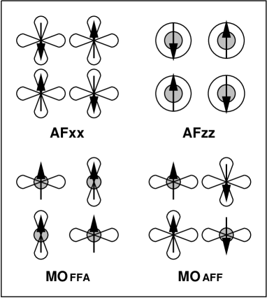
Figure 11: Schematic representation of magnetic and orbital long-range orderings in $(a,b)$ planes for the classical phases: AFxx, AFzz, MOFFA and MOAFF phases. Grey parts of different $e_{g}$ orbitals are oriented along the $c$-axis (after Ref. Ole00 ).

It is clear that at large positive $E_{z}$, where the crystal field strongly favors $|x\rangle$-occupancy over $|z\rangle$-occupancy, one expects that $\theta_{i}=\pi/2$ in Eq. (65), and the holes occupy $|x\rangle$ orbitals at every site. In this case the spins do not interact in the $c$-direction (see Fig. 10), and there is also no orbital energy contribution. Hence, the $(a,b)$ planes will decouple magnetically, while within each plane the superexchange is AF and equal to $9J/4$ along $a$ and $b$. These interactions stabilize a 2D antiferromagnet, called further AFxx phase. On the contrary, if $E_{z}<0$ and $|E_{z}|$ is large, then the holes occupy $|z\rangle$ orbitals and $\theta_{i}=0$ in Eq. (65). By means of the expressions (66) – (69), we find that the spin system has then strongly anisotropic AF superexchange, being $4J$ on the bonds $\langle ij\rangle$ along the $c$-axis, and $J/4$ on the bonds within the $(a,b)$ planes, respectively. This 3D Néel state with the holes occupying $|z\rangle$ orbitals is called AFzz phase. The spin and orbital order in both AF phases is shown schematically within the $(a,b)$ planes in Fig. 11. In this case the energies normalized per one site are given by:

$$E_{\rm AFxx} = -3J\left(1-{\eta\over 4}\right)-{1\over 2}E_{z},$$ (70)

$$E_{\rm AFzz} = -J\left(1+{\eta\over 4}\right)-2J\beta\left(1-{\eta\over 2}\right)+{1\over 2}E_{z}.$$ (71)

The AFxx and AFzz phases are degenerate in a cubic system ($\beta=1$) along the line $E_{z}=0$, while decreasing $\beta$ moves the degeneracy point to negative values of $E_{z}$, given by $E_{z}=-2J(1-\beta)(1-{\eta\over 2})$.

However, for intermediate values of $E_{z}$ one may expect to optimize the energy by realizing mixed orbital configurations ($0<\theta<\pi/2$). In this case, guided by the observation that the orbital interaction is AF-like, we look for solutions with alternating orbitals at two sublattices, $A$ and $B$. The alternation is chosen in a way to allow the orbitals being parallel (optimizing the magnetic energy) in one direction, and being (almost) orthogonal in the other two (optimizing the orbital energy). Such states are realized by choosing in Eq. (65) the angles alternating between two sublattices in particular planes: $\theta_{i}=+\theta$ for $i\in A$, and $\theta_{j}=-\theta$ for $j\in B$, respectively,

$$|i\mu\sigma\rangle = \cos\theta|iz\sigma\rangle+\sin\theta|ix\sigma\rangle,$$

$$|j\mu\sigma\rangle = \cos\theta|jz\sigma\rangle-\sin\theta|jx\sigma\rangle.$$ (72)

Let us assume first the G-AF state. By evaluating the orbital operators following Eqs. (66) – (69) for this case, one finds easily the energy as a function of $\theta$ in Eqs. (III.2),

$$E(\theta) = -\frac{J}{4}(1+\frac{\eta}{2})(7-4\cos^{2}2\theta)-\frac{J}{4}(1-\frac{\eta}{2})(1-2\cos 2\theta)^{2}$$ (73)

$$- \frac{J}{2}\beta(1+\frac{\eta}{2})(1-\cos^{2}2\theta)-\frac{J}{2}\beta(1-\frac{\eta}{2})(1+\cos 2\theta)^{2}+\frac{1}{2}E_{z}\cos 2\theta.$$

This expression has a minimum at

$$\cos 2\theta=-{{(1-\frac{\eta}{2})(1-\beta)+\frac{1}{2}\varepsilon_{z}\over(2+\beta)\eta}},$$ (74)

where $\varepsilon_{z}=E_{z}/J$, if $\eta\neq 0$, and provided that $|\cos 2\theta|\leq 1$ (a similar condition applies to all the other states with MO considered below). So, as long as $2J(\beta-1)-3J(\beta+1)\eta\leq E_{z}\leq 2J(\beta-1)+J(5+\beta)\eta$, there is genuine MO order, while upon reaching the smaller (larger) boundary value for $E_{z}$, the orbitals go over smoothly into $|z\rangle$ ($|x\rangle$), i.e., one retrieves the AFzz (AFxx) phase. Taking the magnetic ordering in the three cubic directions $\{a,b,c\}$ as a label to classify the classical phases with MO (III.2), we call the phase obtained in the regime of genuine MO order MOAAA, with classical energy given by

$$E_{\rm MO{\scriptsize AAA}} = -\left(2+\beta+\frac{3}{4}\eta\right)J-J{\left[(2-\eta)(1-\beta)+\varepsilon_{z}\right]^{2}\over 4(2+\beta)\eta}.$$ (75)

In a similar fashion we can get the MF solutions for other possible spin configurations of A-AF type. Consider first the MOFFA phase, with FM order within the $(a,b)$ planes, and AF order along the $c$-axis. The classical energy as a function of $\theta$ is given by:

$$E(\theta) = -\frac{J}{4}(1+\eta)(7-4\cos^{2}2\theta)-\frac{J}{2}\beta(1+\frac{\eta}{2})(1-\cos^{2}2\theta)$$ (76)

$$-\frac{J}{2}\beta(1-\frac{\eta}{2})(1+\cos 2\theta)^{2}+\frac{1}{2}E_{z}\cos 2\theta,$$

with a minimum at

$$\cos 2\theta={\beta(1-\frac{\eta}{2})-\frac{1}{2}\varepsilon_{z}\over 2+(2+\beta)\eta},$$ (77)

where again the MO exist as long as $|\cos 2\theta|\leq 1$. Using Eqs. (76) and (77) one finds that the classical energy of the MOFFA phase is given by

$$E_{\rm MO{\scriptsize FFA}}=-\frac{J}{4}\left(11-7\eta\right)-\frac{J}{2}{[\beta(1-\frac{\eta}{2})-\frac{1}{2}\varepsilon_{z}]^{2}\over 2+(2+\beta)\eta}.$$ (78)

This solution is stable for $E_{z}<0$, while for $E_{z}>0$ the other two degenerate phases: the MOFAF and MOAFF phase have a lower energy, as they are characterized by a lower hole density in $|z\rangle$ orbitals which become unfavorable. In this case, due to the breaking of local symmetry of the magnetic interactions within the $(a,b)$ planes, with one direction AF and the other FM, one is forced to look for solutions with different angles on the two sublattices Ole00 .

Finally, one may consider how the degeneracy of the AFxx phase is removed by the interactions along the $c$-axis. One possibility is the MOAAA phase, with the energy given above by Eq. (75). If the interactions along the $c$-axis are instead FM, one finds the classical energy of the MOAAF phase given by

$$E_{\rm MO{\scriptsize AAF}}=-\left(2+\frac{3}{4}\eta\right)J-\frac{1}{2}\beta(1+\eta)-J{\left(2-\eta+\varepsilon_{z}\right)^{2}\over 2[\beta(1+\eta)+2\eta]},$$ (79)

with the mixing angle

$$\cos 2\theta=-{{1-\frac{\eta}{2}+\frac{1}{2}\varepsilon_{z}\over\beta(1+\eta)+2\eta}}.$$ (80)

This solution turns out to be stable with respect to the MOAAA as long as $1+\cos 2\theta<\eta$. This means that when the hole density in the $|z\rangle$ orbitals $\sim\cos^{2}\theta$ grows smoothly from zero (at $\theta=\pi/2$) with decreasing $E_{z}$, it tends to stabilize first the MOAAF phase by FM terms $\sim J\eta\cos^{2}\theta$, while at higher occupancy of $|z\rangle$ orbitals the AF interactions $\sim J\cos^{4}\theta$ take over.

Thus, one obtains the classical phase diagram of the 3D spin-orbital model (57) by comparing the energies of the six above phases for various values of two parameters, $E_{z}/J$ and $J_{H}/U$: two AF phases with two sublattices and pure orbital character (AFxx and AFzz), three A-AF phases with four sublattices (MOFFA and two degenerate phases: MOAFF and MOFAF), one C-AF phase (MOAAF), and one G-AF phase with MO’s (MOAAA). By looking at the phase diagram one can see that the generic sequence of classical phases at finite $\eta$ and decreasing $E_{z}/J$ is: AFxx, MOAAF, MOAAA, MOAFF, MOFFA, and AFzz, and the magnetic order is tuned together with the gradually increasing $|z\rangle$ character of the occupied orbitals. By making several other choices of orbital mixing and classical magnetic order, it has been verified that no other commensurate ordering with up to four sublattices can be stable in the present situation. Although some other phases have been found, they were degenerate with the above phases only at the $M=(0,0)$ point of the phase diagram, and otherwise had higher energies.

Figure 12: Mean-field phase diagram of the 3D spin-orbital model (57) in the $(E_{z},J_{H})$ plane for $\beta=1$ (after Ref. Ole00 ). The lines separate the classical states shown in Fig. 11; the transition from AFxx to MOAFF phase is second order (dashed line), while all the other transitions are first order (full lines).

The result for cubic symmetry ($\beta=1$) is presented in Fig. 12, where one finds all six phases, but the MOAAA phase does stabilize only in a very restricted range of parameters for $J_{H}/U<0.1$, in between AFxx and MOAFF phases. Only the first of the above transitions is continuous, while the other lines in Fig. 12 are associated with jumps in the magnetic and in orbital patterns. We would like to emphasize that all the considered phases are degenerate at the $M=(0,0)$ point Fei97 . It is a multicritical point, where the orbitals may be rotated freely when the spins are AF, and a few other states with FM planes, and tuned to them orbital order of the MO type gives precisely the same energy.

When $\beta\neq 1$, the phase diagram changes quantitatively but not qualitatively, with either expanded or reduced areas corresponding to the different classical phases Ole00 . In particular, $\beta>1$ stabilizes the MO phases [especially the MOAFF(MOFAF) states]. On the contrary, the MO phases are stable in a reduced range of $E_{z}$ for a fixed value of $J_{H}/U$, if $\beta<1$. It is worth emphasizing that the multicritical point $M$ is a common feature of the classical phase diagram independently of the value of $\beta$. It follows from the degenerate multiplet structure of $d^{8}$ ions, and its coordinate moves along the $\eta=0$ line, according to the following relation: $E_{z}=-2J(1-\beta)$. This is a clear demonstration of the frustrated nature of the spin and orbital superexchange in the model, whereas the crystal field term just compensates the enhanced or suppressed magnetic interactions in the $(a,b)$ planes.

A special role plays the case with $\beta=0$ which corresponds to the 2D spin-orbital model. In this case the MOAFF phase disappears completely while the other two phases with AF order in the $(a,b)$ planes MOAAA and MOAAF collapse into a single MOAA phase. The resulting phase diagram is shown in Fig. 13. The MOFF is still stable in a large region of the parameter space which demonstrates that the strong AF exchange along the $c$ axis in the corresponding 3D MOFFA phase is not instrumental to stabilize this phase, but the orbital energy within the FM planes is a dominating mechanism.

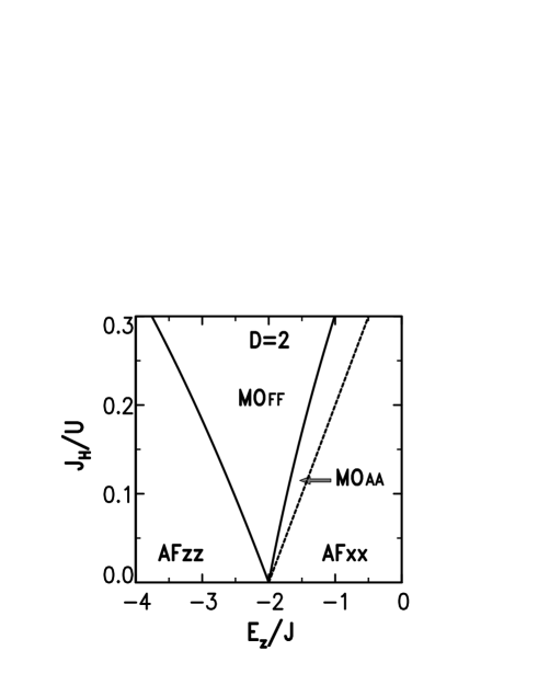
Figure 13: Mean-field phase diagram of the spin-orbital model (57) in the $(E_{z},J_{H})$ plane in two dimensions ($\beta=0$). Full lines separate the classical states AFxx, AFzz, and MOFF shown in Fig. 11, while the spin order in the MOAA phase is AF, and the orbitals are in between those in AFxx and MOFF phase (after Ref. Ole00 )

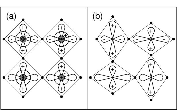
Figure 14: Schematic representation of the mixed orbitals in $(a,b)$ planes of the MOFF phase in a 2D model: (a) the orbitals with their phases, and (b) the resulting distortion in the oxygen lattice, stabilized by the orbital ordering (after Ref. Ole00 )

It is interesting to compare the results obtained on the classical level with some relevant physical systems. For La₂CuO₄ and Nd₂CuO₄ the crystal field splitting is large, $E_{z}\simeq 0.64$ eV Gra92 , so that one falls in the region of the 2D AFxx phase observed in neutron scattering. If on the contrary the orbital splitting is small, the orbital ordering sets in and has to couple strongly to the lattice. The net result is a quadrupolar distortion as indicated in Fig. 14. This lattice instability is again related to the question on the origin of the orbital ordering: is it due to JT and/or to electronic mechanism? The deformations found in KCuF₃ (or LaMnO₃) could in principle be entirely caused by phonon-driven collective JT effects. One might therefore attempt to neglect electron-electron interactions, and focus on the electron-phonon coupling. In case that the ions are characterized by a JT (orbital) degeneracy, one can integrate out the (optical) phonons, and one finds effective Hamiltonians with phonon mediated interactions between the orbitals. In the specific case of $e_{g}$ degenerate ions in a cubic crystal, these look quite similar to the orbital interactions in the $d^{9}$ Hamiltonian, except that the spin dependent term is absent KKphon . Any orbital order resulting from this Hamiltonian is now accompanied by a lattice distortion of the same symmetry.

The size of the quadrupolar deformation in the $(a,b)$ plane of KCuF₃ is actually as large as 4 % of the lattice constant $a_{0}$. It is therefore often argued that the orbital order is clearly phonon-driven, and that the orbital interactions discussed above are less important. Although appealing at first sight, this argument is flawed: large displacements do not necessarily imply that phonons are the driving mechanism. Unfortunately, the deformations of the lattice and the orbital degrees of freedom cannot be disentangled using general principles: they constitute an irreducible subsector of the problem. The issue is therefore a quantitative one, and may be answered by calculating the electronic structure.

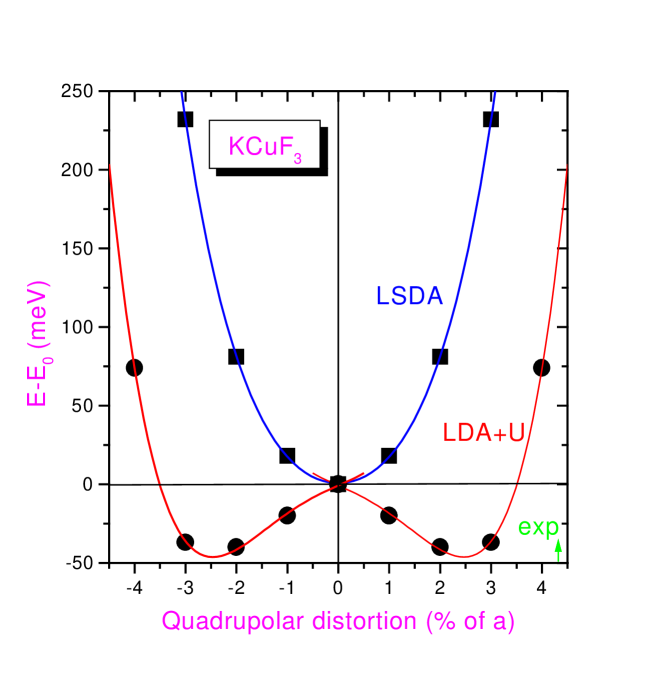
Figure 15: The dependence of the total energy of KCuF₃ on the quadrupolar lattice distortion according to LSDA and LDA+U band structure calculations (after Ref. Lie95 ).

We start out with the observation that according to LDA KCuF₃ would be an undistorted, cubic system: the energy increases if the distortion is switched on (see Fig. 15). The reason is that KCuF₃ would be a band metal according to LDA (the usual Mott-gap problem) with a Fermi-surface which is not susceptible to a band JT instability. Therefore, the effects of strong on-site Coulomb interaction should be included and the LDA+U method Ani91 is a well designed method to serve this purpose. It is constructed to handle the physics of electronic orbital ordering, keeping the accurate treatment of the electron-lattice interaction of LDA intact. According to LDA+U calculations the total energy gained by the deformation of the lattice is only a small contribution of $\sim 50$ meV (Fig. 15) to the energies involved in the electronic orbital ordering Lie95 . Therefore, the coupling to the lattice is here not a driving force for the orbital and magnetic ordering, but the lattice follows the orbital state.

Although the energy gained in the deformation of the lattice is rather small, the electron-phonon coupling is quite effective in keeping KCuF₃ away from the frustrated interactions associated with the origin of the phase diagram (Fig. 12). Since the FM interactions in the $(a,b)$ plane of KCuF₃ are quite small ($J_{(a,b)}=-0.2$ meV, as compared to the ‘1D’ AF exchange $J_{c}=17.5$ meV Ten95 ; Ten95a ; Ten95b ), one might argue that the effective Hund’s rule coupling $J\eta$ as of relevance to the low energy theory is quite small. Such a strong anisotropy of magnetic interactions $J_{(a,b)}$ and $J_{c}$ has been reproduced recently within the ab initio method, but not in unrestricted HF, demonstrating the importance of electron correlation effects. Although this still needs further study, it might well be that in the absence of the electron-phonon coupling KCuF₃ would be close to the origin of Fig. 12. Therefore, although further work is needed to clarify the role played by electron-phonon coupling, it might be that phonons are to a large extent responsible for the stability of KCuF₃’s classical ground state. In any case, one cannot rely just on the size of the lattice deformations to resolve this issue.

III.3 Elementary excitations in the $d^{9}$ model

The presence of the orbital degrees of freedom in the Hamiltonian (57) yields excitation spectra that are qualitatively different from those of the quantum antiferromagnet with a single spin-wave mode. In the present case one gets two transverse excitations: spin waves and spin-and-orbital waves Fei98 ; and also longitudinal excitations – orbital waves, thus producing three elementary excitations for the present spin-orbital model (57) Fei97 ; Ole00 ; Fei98 ; Bri98 . This gives therefore the same number of modes as found in a 1D SU(4) symmetric spin-orbital model (see Sec. IV.A) in the Bethe ansatz method Sut75 ; Fri99 . We emphasize that this feature is a consequence of the dimension (equal to 15) of the $so(4)$ Lie algebra of the local operators, as explained below, and is not related to the global symmetry of the Hamiltonian. In this chapter, we report the analysis of the realistic $d^{9}$ spin-orbital model for the 3D simple cubic (i.e., perovskite-like) lattice (57), using linear spin-wave (LSW) theory Aue94 ; Tak89 , generalized in such a way that makes it applicable to the present situation.

Before we introduce the excitation operators, it is convenient to rewrite the spin-orbital model (57) in a different representation which uses a four-dimensional space: $\{|x\!\uparrow\rangle$, $|x\!\downarrow\rangle$, $|x\!\downarrow\rangle\}$, $|z\!\uparrow\rangle$, instead of a direct product of the spin and orbital subspaces. This will demonstrate explicitly that three different elementary excitations appear in a natural way. Hence, we introduce operators which define purely spin excitations in individual orbitals,

$$S^{+}_{ixx}=d^{\dagger}_{ix\uparrow}d_{ix\downarrow},\hskip 34.14322ptS^{+}_{izz}=d^{\dagger}_{iz\uparrow}d_{iz\downarrow},$$ (81)

and operators for simultaneous spin-flip and transfer between the orbitals, spin-and-orbital excitations,

$$K^{+}_{ixz}=d^{\dagger}_{ix\uparrow}d_{iz\downarrow},\hskip 28.45274ptK^{+}_{izx}=d^{\dagger}_{iz\uparrow}d_{ix\downarrow}.$$ (82)

The corresponding operators $S^{z}_{i\alpha\alpha}$ and $K^{z}_{i\alpha\beta}$ are defined as follows,

$$S^{z}_{ixx} = \frac{1}{2}(n_{ix\uparrow}-n_{ix\downarrow}),\hskip 65.44142ptS^{z}_{izz}=\frac{1}{2}(n_{iz\uparrow}-n_{iz\downarrow}),$$ (83)

$$K^{z}_{ixz} = \frac{1}{2}(d^{\dagger}_{ix\uparrow}d_{iz\uparrow}-d^{\dagger}_{ix\downarrow}d_{iz\downarrow}),\hskip 28.45274ptK^{z}_{izx}=\frac{1}{2}(d^{\dagger}_{iz\uparrow}d_{ix\uparrow}-d^{\dagger}_{iz\downarrow}d_{ix\downarrow}).$$ (84)

The Hamiltonian (57) contains also purely orbital interactions which can be expressed using the following orbital excitation operators,

$$T_{ixz} = \frac{1}{2}(d^{\dagger}_{ix\uparrow}d_{iz\uparrow}+d^{\dagger}_{ix\downarrow}d_{iz\downarrow}),\hskip 28.45274ptT_{izx}=\frac{1}{2}(d^{\dagger}_{iz\uparrow}d_{ix\uparrow}+d^{\dagger}_{iz\downarrow}d_{ix\downarrow}),$$ (85)

while the anisotropy in the orbital space is expressed by orbital-polarization operators,

$$n_{i-}=\frac{1}{2}(d^{\dagger}_{ix\uparrow}d_{ix\uparrow}\!+d^{\dagger}_{ix\downarrow}d_{ix\downarrow}\!-\!d^{\dagger}_{iz\uparrow}d_{iz\uparrow}\!-\!d^{\dagger}_{iz\downarrow}d_{iz\downarrow}).$$ (86)

In order to simplify the notation, we also introduce global operators for the spin, spin-and-orbital and orbital excitations,

$$S^{+}_{i} = S^{+}_{ixx}+S^{+}_{izz},\hskip 28.45274ptS^{z}_{i}=S^{z}_{ixx}+S^{z}_{izz},$$ (87)

$$K^{+}_{i} = K^{+}_{ixz}+K^{+}_{izx},\hskip 28.45274ptK^{z}_{i}=K^{z}_{ixz}+K^{z}_{izx},$$ (88)

$$T_{i} = T_{ixz}+T_{izx}.$$ (89)

The number of collective modes in a particular phase may be determined as follows. The $so(4)$ Lie algebra consists of three Cartan operators, i.e., operators diagonal on the local basis of the symmetry-broken phase under consideration (e.g. $S^{z}_{ixx}$, $S^{z}_{izz}$, and $n_{i-}$ in the AFxx phase), plus twelve nondiagonal operators turning the eigenstates into one another (like $S^{+}_{ixx}$ and $S^{+}_{izz}$ in the AFxx phase). Out of those twelve operators, six connect two excited states (like $S^{+}_{izz}$ in the AFxx phase), and are physically irrelevant (in the lowest order), because they give only rise to the so-called ’ghost’ modes, the modes for which the spectral function vanishes identically at $T=0$. The remaining six operators connect the local ground state with excited states, three of them describing an excitation and three a deexcitation, and only these six operators are physically relevant. Out of the three excitations (deexcitations), two are transverse, i.e., change the spin, and one is longitudinal, i.e., does not affect the spin. For a classical phase with $L$ sublattices one therefore expects $4L$ transverse and $2L$ longitudinal modes. Because of time-reversal invariance they all occur in pairs with opposite frequencies, $\pm\omega^{(n)}_{\vec{k}}$.

Finally, the SU(2) spin invariance of the Hamiltonian guarantees that the transverse operators raising the spin are decoupled from those lowering the spin, and that both sets of operators are described by equivalent equations of motion, so that the transverse modes are pairwise degenerate. Such a simplification does not occur in the longitudinal sector. So, in conclusion, in an $L$-sublattice phase there are $L$ doubly-degenerate positive-frequency transverse modes and $L$ nondegenerate positive-frequency longitudinal modes, accompanied by the same number of negative-frequency modes. This may be compared with the well-known situation in the quantum antiferromagnet Aue94 , where there is, with only spin excitation operators involved, only one (not two) doubly-degenerate positive-frequency (transverse) mode and the corresponding negative-frequency mode in the two-sublattice Néel state.

For the actual evaluation it is convenient to decompose the superexchange terms (58) in the spin-orbital Hamiltonian (57),

$${\cal H}_{J}={\cal H}_{\parallel}+{\cal H}_{\perp},$$ (90)

into two parts which depend on the bond direction:

(i) for the bonds $\langle ij\rangle\parallel(a,b)$,

$${\cal H}_{\parallel} = \frac{1}{4}J\sum_{\langle ij\rangle{\parallel}}\left[(1-\frac{1}{2}\eta)(3{\vec{S}}_{ixx}+{\vec{S}}_{izz}+\lambda_{ij}\sqrt{3}{\vec{K}}_{i})\cdot(3{\vec{S}}_{jxx}+{\vec{S}}_{jzz}+\lambda_{ij}\sqrt{3}{\vec{K}}_{j})\right.$$ (91)

$$\left.\hskip 31.2982pt-2\eta{\vec{S}}_{i}\cdot{\vec{S}}_{j}+(1+2\eta)(n_{i-}+\pm\sqrt{3}T_{i})(n_{j-}+\pm\sqrt{3}T_{j})-(3+\eta)\right],$$

(ii) for the bonds $\langle ij\rangle\perp(a,b)$, i.e., along the $c$-axis,

$${\cal H}_{\perp} = J\sum_{\langle ij\rangle{\perp}}[(4-2\eta){\vec{S}}_{izz}\cdot{\vec{S}}_{jzz}-\eta({\vec{S}}_{ixx}\cdot{\vec{S}}_{jzz}+{\vec{S}}_{izz}\cdot{\vec{S}}_{jxx})$$ (92)

$$\hskip 28.45274pt+(1+2\eta)n_{i-}n_{j-}-\frac{1}{4}(3+\eta)].$$

Here and in the following paragraphs we consider a 3D cubic model with $\beta=1$. We note that the orbital interactions (82) are quite different in $H_{\parallel}$ and $H_{\perp}$; propagating composite spin-and-orbital excitations are possible only within the $(a,b)$ planes, where they are coupled to the spin excitations, while in the $c$-direction only pure spin excitations and pure spin-and-orbital excitations occur, which are decoupled from one another. This apparent breaking of symmetry between $H_{\parallel}$ and $H_{\perp}$ is a consequence of the choice of basis as $|x\rangle$ and $|z\rangle$ orbitals.

In the following, we report briefly the results obtained for transverse and longitudinal excitations in the various symmetry-broken classical states of the spin-orbital model (57). The transverse excitations, i.e., spin-waves and spin-and-orbital-waves, are calculated using the spin-rising operators which make a transition to a state realized in a classical phase at a given site $i$. As an example we use the AFxx phase to illustrate the formalism and calculation method with the excitation operators:

$$S^{+}_{ixx}=d^{\dagger}_{ix\uparrow}d_{ix\downarrow},\hskip 28.45274ptK^{+}_{ixz}=d^{\dagger}_{ix\uparrow}d_{iz\downarrow}.$$ (93)

The longitudinal excitations (without spin-flip) are most conveniently obtained starting from spin-dependent orbital excitation operators,

$$T_{ixz\sigma}=d^{\dagger}_{ix\sigma}d_{iz\sigma},\hskip 28.45274ptT_{izx\sigma}=d^{\dagger}_{iz\sigma}d_{ix\sigma},$$ (94)

as these excitations conserve the spin component and we ask a question whether such a longitudinal excitation may propagate coherently in a given symmetry-broken classical state.

The nature and dispersion of elementary excitations in the spin-orbital model (57) can be conveniently studied in the leading order of the $1/S$ expansion using the Green function formalism. The starting point are the equations of motion for the Green functions generated by the excitation operators (93) written in the energy representation Zub60 ; Hal72 ,

$$E\langle\langle S_{ixx}^{+}|...\rangle\rangle = {1\over 2\pi}\langle[S_{ixx}^{+},...]\rangle+\langle\langle[S_{ixx}^{+},H]|...\rangle\rangle,$$ (95)

$$E\langle\langle K_{ixz}^{+}|...\rangle\rangle = {1\over 2\pi}\langle[K_{ixz}^{+},...]\rangle+\langle\langle[K_{ixz}^{+},H]|...\rangle\rangle,$$ (96)

where the average of the commutator on the right hand side, e.g. $\langle[S_{ixx}^{+},S_{jxx}^{-}]\rangle$, is evaluated in the classical ground state. We note, however, that equivalent results for the AFxx and AFzz phases can be obtained using instead an expansion around a classical saddle point with Schwinger bosons Aue94 .

The equations of motion have been derived for the Green functions generated by the set of operators $\{S_{ixx}^{+},K_{ixz}^{+},S_{jxx}^{+},K_{jxz}^{+}\}$, where $i\in A$ and $j\in B$, and used the random-phase approximation (RPA) for spinlike operators which linearizes the equations of motion by a decoupling procedure Zub60 ; Hal72 . Thereby, the operators which have nonzero expectation values in the considered classical state give finite contributions, e.g. for the first spin-flip Green function one uses,

$$\langle\langle S_{ixx}^{+}S_{mxx}^{z}|...\rangle\rangle\simeq\langle S_{mxx}^{z}\rangle\langle\langle S_{ixx}^{+}|...\rangle\rangle,$$ (97)

and a similar formula for the mixed spin-and-orbital excitation described by $\langle\langle K_{ixz}^{+}|...\rangle\rangle$,

$$\langle\langle K_{ixz}^{+}S_{mxx}^{z}|...\rangle\rangle\simeq\langle S_{mxx}^{z}\rangle\langle\langle K_{ixz}^{+}|...\rangle\rangle.$$ (98)

In the present case of the AFxx phase one uses the respective Néel state average values,

$$\langle S_{ixx}^{z}\rangle = -\langle S_{jxx}^{z}\rangle=\frac{1}{2},$$ (99)

$$\langle n_{i-}\rangle = \langle n_{j-}\rangle=\frac{1}{2},$$ (100)

where $i\in A$ and $j\in B$, and $A$ and $B$ are the two sublattices in a 2D lattice of the AFxx phase, and all the remaining averages vanish. It is crucial that the decoupled operators have different site indices, and thus the decoupling procedure preserves the local commutation rules. Instead, if one uses products of spin and orbital operators, e.g., $K_{ixz}^{+}=S_{ixx}^{+}\sigma_{i}^{+}$, one is tempted to decouple these operators locally Cas78 ; Kha97 which would violate the algebraic structure of the $so(4)$ Lie algebra.

The translational invariance of the Néel state implies that the transformed Green functions are diagonal in the reduced Brillouin zone (BZ). As in the Heisenberg antiferromagnet, the Fourier transformed functions are defined for the Green functions which describe the spin dynamics on a given sublattice, either $A$ or $B$. For instance, the pure spin-flip Green functions are transformed as follows,

$$\langle\langle S_{{\vec{k}}xx}^{+}|...\rangle\rangle_{A} = \frac{1}{\sqrt{N}}\sum_{i\in A}e^{i{\vec{k}}{\vec{R}}_{i}}\langle\langle S_{ixx}^{+}|...\rangle\rangle_{A},$$

$$\langle\langle S_{{\vec{k}}xx}^{+}|...\rangle\rangle_{B} = \frac{1}{\sqrt{N}}\sum_{j\in B}e^{i{\vec{k}}{\vec{R}}_{j}}\langle\langle S_{jxx}^{+}|...\rangle\rangle_{B},$$ (101)

where $N$ is the number of sites in one sublattice. Hence, the problem of finding the elementary excitations of the considered spin-orbital model (57) reduces to the diagonalization of the following $4\times 4$ dynamical matrix at each ${\vec{k}}$-point:

$$\left(\begin{array}[]{cccc}\lambda_{\alpha}-\overline{\omega}_{\vec{k}}&0&Q_{\alpha\vec{k}}&P_{\alpha\vec{k}}\\ 0&\tau_{\alpha}-\overline{\omega}_{\vec{k}}&P_{\alpha\vec{k}}&R_{\vec{k}}\\ -Q_{\alpha\vec{k}}&-P_{\alpha\vec{k}}&-\lambda_{\alpha}-\overline{\omega}_{\vec{k}}&0\\ -P_{\alpha\vec{k}}&-R_{\vec{k}}&0&-\tau_{\alpha}-\overline{\omega}_{\vec{k}}\end{array}\right)\left(\begin{array}[]{c}\langle\langle S^{+}_{{\vec{k}}xx}|\cdots\rangle\rangle_{A}\\ \langle\langle K^{+}_{{\vec{k}}xz}|\cdots\rangle\rangle_{A}\\ \langle\langle S^{-}_{{\vec{k}}xx}|\cdots\rangle\rangle_{B}\\ \langle\langle K^{-}_{{\vec{k}}xz}|\cdots\rangle\rangle_{B}\end{array}\right)=0,$$ (102)

The symmetric positive and negative eigenvalues $\pm\omega_{\vec{k}}^{(n)}$, with $n=1,2$, solved from the matrix in Eq. (102) may be written in the following form for the AFxx phase,

$$[\omega_{\vec{k}}^{(n)}]^{2} = J^{2}\left(\lambda_{x}^{2}+\tau_{x}^{2}-Q_{x\vec{k}}^{2}-R_{\vec{k}}^{2}-2P_{x\vec{k}}^{2}\right)\pm J^{2}\left[(\lambda_{x}^{2}-\tau_{x}^{2})^{2}-2(\lambda_{x}^{2}-\tau_{x}^{2})(Q_{x\vec{k}}^{2}-R_{\vec{k}}^{2})\right.$$ (103)

$$- \left.4(\lambda_{x}-\tau_{x})^{2}P_{x\vec{k}}^{2}+(Q_{x\vec{k}}^{2}+R_{\vec{k}}^{2}+2P_{x\vec{k}}^{2})^{2}-4(Q_{x\vec{k}}R_{\vec{k}}-P_{x\vec{k}}^{2})^{2}\right]^{1/2}.$$

Here the quantities $\lambda_{x}$ and $\tau_{x}$ play the role of local potentials and follow from the model parameters, $E_{z}$ and $J_{H}$,

$$\lambda_{x} = \frac{9}{2}-3\eta,$$ (104)

$$\tau_{x} = \frac{7}{2}-4\eta-2-\eta+\varepsilon_{z}.$$ (105)

The remaining terms are ${\vec{k}}$-dependent, and depend on

$$\gamma_{+}(\vec{k}) = \frac{1}{2}(\cos k_{x}+\cos k_{y}),$$ (106)

$$\gamma_{-}(\vec{k}) = \frac{1}{2}(\cos k_{x}-\cos k_{y}),$$ (107)

$$\gamma_{z}(\vec{k}) = \cos k_{z}.$$ (108)

The quantities $Q_{x\vec{k}}$ and $P_{x\vec{k}}$ for the AFxx phase take the form,

$$Q_{x\vec{k}} = (\frac{9}{2}-3\eta)\gamma_{+}(\vec{k}),$$ (109)

$$P_{x\vec{k}} = \frac{1}{2}\sqrt{3}(3-\eta)\gamma_{-}(\vec{k}),$$ (110)

while the last dispersive term,

$$R_{\vec{k}}=\frac{3}{2}\gamma_{+}(\vec{k}),$$ (111)

carries no index and remains identical for both G-AF phases (AFxx and AFzz). We emphasize that the coupling between the spin-wave and spin-and-orbital-wave excitations occurs due to the terms $\propto P_{x\vec{k}}$, as seen from Eq. (102). It vanishes in the planes of $k_{x}=\pm k_{y}$, but otherwise plays an important role, as discussed in Sec. III. In the limit of large $E_{z}\to\infty$, Eq. (103) reproduces the spin-wave excitations for a 2D antiferromagnet with an AF superexchange interaction of $J(\frac{9}{4}-\frac{3}{2}\eta)$, as given between the occupied $|x\rangle$ orbitals,

$$\omega_{\vec{k}}^{(1)}=J\left(\frac{9}{2}-3\eta\right)[1-\gamma_{+}^{2}(\vec{k})]^{1/2},$$ (112)

while the dispersion of the high-energy spin-and-orbital excitation, $\omega_{\vec{k}}^{(2)}\simeq E_{z}$, becomes negligible. As explained above, both modes are doubly degenerate.

Consider now the orbital (excitonic) excitations generated by the orbital-flip operators (85). They are found by considering the equations of motion,

$$E\langle\langle T_{i\alpha\beta\sigma}|...\rangle\rangle={1\over 2\pi}\langle[T_{i\alpha\beta\sigma},...]\rangle+\langle\langle[T_{i\alpha\beta\sigma},H]|...\rangle\rangle,$$ (113)

where spin $\sigma$ corresponds to the occupied state in the symmetry-broken Néel state. By making a Fourier transformations as for the transverse operators (101), one may show that only two operators per sublattice suffice to describe the modes in an antiferromagnet. The structure of the respective RPA dynamical matrix is given by

$$\left(\begin{array}[]{cccc}u_{\alpha}-\overline{\zeta}_{\vec{k}}&0&+\rho_{\alpha\vec{k}}&+\rho_{\alpha\vec{k}}\\ 0&-u_{\alpha}-\overline{\zeta}_{\vec{k}}&-\rho_{\alpha\vec{k}}&-\rho_{\alpha\vec{k}}\\ -\rho_{\alpha\vec{k}}&-\rho_{\alpha\vec{k}}&-u_{\alpha}-\overline{\zeta}_{\vec{k}}&0\\ +\rho_{\alpha\vec{k}}&+\rho_{\alpha\vec{k}}&0&u_{\alpha}-\overline{\zeta}_{\vec{k}}\end{array}\right)\left(\begin{array}[]{c}\langle\langle T_{{\vec{k}}xz\uparrow}|\cdots\rangle\rangle_{A}\\ \langle\langle T_{{\vec{k}}zx\uparrow}|\cdots\rangle\rangle_{A}\\ \langle\langle T_{{\vec{k}}xz\downarrow}|\cdots\rangle\rangle_{B}\\ \langle\langle T_{{\vec{k}}zx\downarrow}|\cdots\rangle\rangle_{B}\end{array}\right)=0,$$ (114)

with

$$u_{x} = \varepsilon_{z}-3\eta,$$ (115)

$$\rho_{x\vec{k}} = \frac{3}{2}\eta\gamma_{+}(\vec{k}),$$ (116)

and one finds two, in general nondegenerate, positive-frequency modes,

$$\zeta_{\vec{k}}=J\;\left[u_{\alpha}(u_{\alpha}\pm 2\rho_{\alpha\vec{k}})\right]^{1/2}.$$ (117)

It is important to realize that the propagation of longitudinal excitations, being equivalent to a finite dispersion of longitudinal modes, becomes possible only at $\eta>0$. This follows from the multiplet structure of the excited $d^{8}$ states, which allows a spin-flip between the orbitals in the $|^{1}E_{\theta}\rangle$ and in the $S^{z}=0$ component of the $|^{3}A_{2}\rangle$-state only if $J_{H}\neq 0$, as illustrated in Fig. 16. The processes $\sim t_{xz}$ are not shown, as they would also lead to a final state given in Fig. 16(b), i.e., to a propagation of a spin-and-orbital excitation which was already considered above. In contrast, the relevant longitudinal orbital excitation in the symmetry-broken state implies that the exciton has the same spin as imposed by the Néel state of the background; this state is shown in Fig. 16(c). Therefore, in a perfect Néel state without FM interactions due to $\eta\neq 0$, only local orbital excitations are possible. These local excitations cost no energy in the limit of $\varepsilon_{z}\to 0$ which demonstrates again the frustration of magnetic interactions at the classical degeneracy point, $\varepsilon_{z}=\eta=0$.

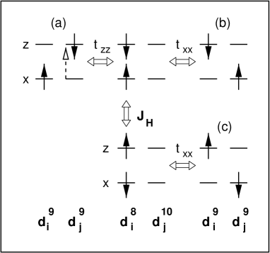
Figure 16: Schematic propagation of the orbital (excitonic) excitation (a). If $J_{H}=0$, an orbital excitation can propagate only to state (b) and is accompanied by a spin-flip (top), while $J_{H}>0$ allows also the spin-flip in the intermediate $d_{i}^{8}$ state, and thus the propagation without spin-flip (c) becomes possible (bottom) (after Ref. Ole00 ).

Figure 17: Spin-wave and spin-and-orbital-wave transverse excitations (full lines) and longitudinal excitations (dashed lines) in AFxx phase (bottom), and neutron intensities of the transverse excitations (top). Parameters: $E_{z}/J=3.0$ and $J_{H}/U=0.3$ (after Ref. Ole00 ).

An example of the excitation spectra is presented in Fig. 17 for the main directions in the 2D BZ, with $X=(\pi,0)$ and $S=(\pi/2,\pi/2)$. Near the $\Gamma$ point one finds a (doubly-degenerate) Goldstone mode $\omega_{\vec{k}}^{(1)}$ with dispersion $\sim k$ at ${\vec{k}}\to 0$, as in the Heisenberg antiferromagnet, and a second (doubly-degenerate) transverse mode at higher energy, $\omega_{\vec{k}}^{(2)}\simeq\omega_{0}+ak^{2}$. Near the $\Gamma$ point the Goldstone mode is essentially purely spin-wave, the second mode is purely spin-and-orbital wave. With increasing ${\vec{k}}$ these modes start to mix due to the $P_{x{\vec{k}}}$ term along the $\Gamma-X$ direction. This is best illustrated by the intensity measured in the neutron scattering experiments, which see only the spin-wave component in each transverse mode. Indeed, the intensity $\chi({\vec{q}})$ is transferred from one mode to the other along the $\Gamma-X$ direction in the 2D BZ (Fig. 17), demonstrating that indeed the lowest (highest) mode is predominantly spin-wave-like (spin-and-orbital-wave-like) before the anticrossing point, while this is reversed after the anticrossing of the two modes. Thus, we make here a specific prediction that two spin-wave-like modes could be measurable in certain parts of the 2D BZ, in particular in the vicinity of the anticrossing, if only an AFxx phase was realized for parameters not too distant from the classical degeneracy point.

Unfortunately, for the realistic parameters for the cuprates Gra92 , one finds $E_{z}/J\simeq 10$ which makes the spin-and-orbital excitation and the changes of the spin-wave dispersion hardly visible in neutron spectroscopy. The orbital (longitudinal) excitations are found for the parameters of Fig. 17 at a finite energy, being of the same order of magnitude as the energy of the spin-and-orbital excitation, $\omega^{(2)}_{\vec{k}}$. The weak dispersion of these modes follows from the spin-flip processes in the excited states, as explained in Fig. 16 and discussed above. We emphasize that the orbital mode has a gap and does not couple to any spin excitation. At the classical degeneracy point $M$ the orbital mode falls to zero energy and is dispersionless, expressing that the orbital can be changed locally without any cost in energy.

The transverse excitations in the AFzz phase are determined by considering the complementary set of Green functions to that given by Eqs. (95) and (96), with the excitation operators $S_{izz}^{+}$ and $K_{izx}^{+}$. After deriving the RPA equations, one finds the final form of the equations of motion by performing a Fourier transformation and using the following nonvanishing expectation values,

$$\langle S_{izz}^{z}\rangle = -\langle S_{jzz}^{z}\rangle=\frac{1}{2},$$ (118)

$$\langle n_{i-}\rangle = \langle n_{j-}\rangle=-\frac{1}{2},$$ (119)

in the AFzz phase, with $i\in A$ and $j\in B$. This leads again to the general form (102), with the elements $\lambda_{x}$, $\tau_{x}$, $Q_{x\vec{k}}$, and $P_{x\vec{k}}$ now replaced by,

$$\lambda_{z} = \frac{1}{2}-\eta+2(2-\eta),$$ (120)

$$\tau_{z} = -\frac{1}{2}-\eta+2(1-2\eta)-\varepsilon_{z},$$ (121)

$$Q_{z\vec{k}} = (\frac{1}{2}-\eta)\gamma_{+}(\vec{k})+2(2-\eta)\gamma_{z}(\vec{k}),$$ (122)

$$P_{z\vec{k}} = \frac{1}{2}\sqrt{3}(1-\eta)\gamma_{-}(\vec{k}).$$ (123)

Thus, the transverse excitations have the same form (103) as in the AFxx phase, but the above quantities (120)–(123) have to be used.

In the limit of large $E_{z}\to-\infty$ one finds the spin-wave for a 3D anisotropic antiferromagnet with strong superexchange equal to $2J(2-\eta)$ along the $c$-axis, and weak superexchange $\frac{1}{4}J(1-2\eta)$ within the $(a,b)$-planes,

$$\omega_{\vec{k}}^{(1)}=J\left\{\left[(\frac{1}{2}-\eta)+2(2-\eta)\right]^{2}-\left[(\frac{1}{2}-\eta)\gamma_{+}(\vec{k})+2(2-\eta)\gamma_{z}\right]^{2}\right\}^{1/2},$$ (124)

while the spin-and-orbital excitation, $\omega_{\vec{k}}^{(2)}\simeq-E_{z}$, is dispersionless. Again, both these transverse modes are doubly degenerate.

The representative excitation spectrum for the AFzz phase may be found in Ref. Ole00 . One finds again a Goldstone mode $\omega_{\vec{k}}^{(1)}$ at the $\Gamma$ point which is spin-wave-like, accompanied by a finite energy spin-and-orbital mode $\omega_{\vec{k}}^{(2)}$. The first one is linear, while the second changes quadratically with increasing ${\vec{k}}$. The dispersion in the $\Gamma-X$ direction is, however, only $\sim 0.7J$, while in the AFxx phase a large dispersion of $\sim 2.5J$ was found. This demonstrates the large difference between the superexchange in the $(a,b)$-planes in these two AF phases. Here one should bear in mind, that in a strongly anisotropic antiferromagnet, such as the AFzz phase, the dispersion of the spin-wave mode in the $(k_{x},k_{y})$ plane is roughly given by $(zJ_{ab}J_{c})^{1/2}S$, so actually enhanced by $(J_{c}/zJ_{ab})^{1/2}$ compared with the planar exchange constant.

The (longitudinal) orbital excitations in the AFzz phase are found using the equations of motion of the form (113) which lead to Eq. (114) with,

$$u_{z} = -\varepsilon_{z}-3\eta,$$ (125)

$$\rho_{z\vec{k}} = -\frac{3}{2}\eta\gamma_{+}(\vec{k}),$$ (126)

and we find again zero-energy nondispersive modes at $\varepsilon_{z}=\eta=0$. The orbital excitation is found at the $X=(\pi,0,0)$ and $L=(\pi/2,\pi/2,\pi/2)$ points at the same energy as that of a local excitation from $|z\rangle$ to $|x\rangle$ orbital. It depends only on the energy difference between the orbitals, and has a weak dispersion $\sim J\eta$ due to the same mechanism as described above for the AFxx phase (Fig. 16).

The excitation operators which couple to the local states in the MOFFA phase with mixed orbitals are linear combinations of the operators considered above. It is therefore convenient to make a unitary transformation of the Hamiltonian (57) to new orbitals defined as follows for $i\in A$ or $i\in D$ sublattice,

$$\left(\begin{array}[]{c}|i\mu\rangle\\ |i\nu\rangle\end{array}\right)=\left(\begin{array}[]{cc}\cos\theta&\sin\theta\\ -\sin\theta&\cos\theta\end{array}\right)\left(\begin{array}[]{c}|iz\rangle\\ |ix\rangle\end{array}\right),$$ (127)

and for $j\in B$ or $j\in C$ sublattice,

$$\left(\begin{array}[]{c}|j\mu\rangle\\ |j\nu\rangle\end{array}\right)=\left(\begin{array}[]{cc}\cos\theta&-\sin\theta\\ \sin\theta&\cos\theta\end{array}\right)\left(\begin{array}[]{c}|jz\rangle\\ |jx\rangle\end{array}\right).$$ (128)

With these definitions and by choosing the angle $\theta$ at the value which minimizes the classical energy (77), we guarantee that $|i\mu\rangle$ and $|j\mu\rangle$, respectively, are the orbital states realized in the classical MOFFA phase at each site, which is G-type with respect to the orbital ordering, while $|i\nu\rangle$ and $|j\nu\rangle$ are the excited states, so that one can readily define the excitation operators pertinent to the symmetry-broken ground state of this phase.

Figure 18: The same as in Fig. 17, but for the MOFFA phase, as obtained for $E_{z}/J=-1.0$ and $J_{H}/U=0.3$. Different modes are labelled by the increasing indices $i=1,\dots,4$ with increasing energy (after Ref. Ole00 ).

Thus the spin ${\cal S}_{i\mu\mu}^{+}$, spin-and-orbital ${\cal K}_{i\mu\nu}^{+}$, and orbital ${\cal T}_{i\mu\nu\sigma}$ operators are defined in terms of the new reference orbital states $\{|\mu\rangle,|\nu\rangle\}$, and fulfill the same commutation rules as the non-transformed operators: $S_{i\alpha\alpha}^{+}$ $K_{i\alpha\beta}^{+}$, and $T_{i\alpha\beta\sigma}$, respectively. To simplify the notation we also introduce total spin ${\cal S}_{i}^{+}$ and spin-and-orbital ${\cal K}_{i}^{+}$ operators, as explained above. The Hamiltonian (57) has to be transformed by the inverse transformations to those given by Eqs. (127) and (128) Ole00 . Hence, the transverse excitations may be found starting from the relevant raising operators that lead to the local state $|i\mu\uparrow\rangle$ realized in one of the sublattices, analogous to those introduced for the AFxx phase (93), i.e., the set $\{{\cal S}_{i\mu\mu}^{+},{\cal K}_{i\mu\nu}^{+},{\cal S}_{j\mu\mu}^{+},{\cal K}_{j\mu\nu}^{+},{\cal S}_{k\mu\mu}^{+},{\cal K}_{k\mu\nu}^{+},{\cal S}_{l\mu\mu}^{+},{\cal K}_{l\mu\nu}^{+}\}$, where $i\in A$, $j\in B$, $k\in C$, and $l\in D$; they lead as usual to the orbitals $\{|i\mu\rangle,|j\mu\rangle\}$ (III.2) realized in the MOFFA phase. We applied the same RPA procedure as explained above for the AFxx and AFzz phase in order to determine the Green function equations in the ${\vec{k}}$-space. The longitudinal excitations can be obtained from operators ${\cal T}_{i\mu\nu\sigma}$ similar to those used in the AFxx and AFzz phases (94), taking $\sigma=\uparrow$ for the $(a,b)$ planes occupied with $\uparrow$-spins, and $\sigma=\downarrow$ for the $(a,b)$ planes occupied with $\downarrow$-spins. As expected, there are four doubly-degenerate positive-frequency transverse modes, and four non-degenerate positive-frequency longitudinal modes, consistent with the MOFFA phase having four sublattices.

An example of the transverse and longitudinal modes in the MOFFA phase is presented in Fig. 18. The modes are shown in the respective BZ which corresponds to the magnetic unit cell of the MOFFA phase: The 2D part along $\Gamma-X-S-\Gamma$ resembles the modes in the AFxx phase (compare Fig. 17), reflecting the orbital alternation, while the AF coupling along the $c$-axis results in the folding of the zone along the $\Gamma-Z$ direction, with $Z^{\prime}=(0,0,\pi/2)$ and $S^{\prime}=(\pi/2,\pi/2,\pi/2)$. One finds one Goldstone mode, and three other finite-energy modes at the $\Gamma$ point. If no AF coupling along the $c$-axis is present, similar positive-energy modes describe the excitation spectrum in the MOFF phase in the 2D part of the BZ (in the region of stability shown in Fig. 13), and the symmetric negative-frequency modes carry then no weight. In contrast, due to the strong AF interactions in the MOFFA phase, the negative modes give a large energy renormalization due to quantum fluctuations, as discussed in more detail in Sec. IV.B.

The spin-wave and spin-and-orbital-wave excitations are well separated along the $\Gamma-X-S-\Gamma$ path, with a gap of $\sim 0.5J$, as the FM interactions $\propto J\eta$ are considerably weaker than the orbital interactions which are $\propto J$. Therefore, the neutron intensity $\chi({\vec{q}})$ is found mainly as originating from the lowest energy mode, $\omega_{\vec{k}}^{(1)}$, with a small admixture of the higher-energy spin-and-orbital excitation, $\omega_{\vec{k}}^{(3)}$. The magnetic interactions are considerably stronger along the $c$-axis; the modes mix and the higher-energy excitations, $\omega_{\vec{k}}^{(n)}$ with $n=3,4$, have a larger dispersion in the remaining directions with $k_{z}\neq 0$. Strong mixing of the modes in this part of the BZ is also visible in the intensity distribution, with the modes $n=1$ and $n=3$ contributing with comparable intensities (Fig. 18). The fact that modes labeled as 2 and 4 have zero intensity is due to the path $\Gamma-Z^{\prime}-S^{\prime}-\Gamma$ being in the high-symmetry BZ plane where $k_{x}=k_{y}$ so that $\gamma_{-}(\vec{k})=0$. Then modes 2 and 4 have equal amplitude but are exactly out-of-phase between $A$ and $B$ sites as well as between $C$ and $D$ sites, and so their neutron intensities vanish, and only the companion in-phase modes 1 and 3 are observable by neutrons. Unlike in the AF phases, the purely orbital excitation is here energetically separated from the spin wave and spin-and-orbital wave. The dispersion is quite small and decreases with $\eta$.

Interestingly, although the order in the $(a,b)$ planes is FM, the energy of the Goldstone mode increases linearly in all three directions with increasing ${\vec{k}}$, and the slopes are proportional to the respective exchange interactions. This behavior is a manifestation of the A-AF spin order; a qualitatively similar spectrum is found experimentally in LaMnO₃ Hir96 ; Hir96a , where, however, the excitation spectra correspond to large spins $S=2$ of Mn³⁺ ions. The rather small dispersion of the spin-wave part at low energies is due to small values of the exchange constants for the actual optimal orientation of orbitals found at $J_{H}/U=0.3$. We note, however, that the AF interactions along the $c$-axis are much stronger at $J_{H}\to 0$ than in the present case. The AF structure along the $c$-axis may be easily recognized from the symmetric spin-wave mode in the $\Gamma-Z$ direction with respect to $Z^{\prime}=(0,0,\pi/2)$, while this mode increases all the way from the $\Gamma$ to the $X$ point. Unfortunately, no experimental verification of these spectra is possible at present, as the spin excitations measured in neutron scattering for KCuF₃ are consistent with the Bethe ansatz and thus suggest a spin-liquid ground state with strong 1D AF correlations instead of the A-AF phase with magnetic LRO Ten95 ; Ten95a ; Ten95b .

The elementary excitations in the MOAFF phase may be obtained using a similar scheme to that described here for the MOFFA phase. In this case, the transverse excitations have a similar dependence on the ${\vec{k}}$-vector to those found in the MOFFA phase, but the value of the crystal-field $E_{z}$ is effectively smaller by a factor of two in comparison with the MOFFA phase. This asymmetry is a consequence of the choice of $|x\rangle$ and $|z\rangle$ states as orbital basis to which $E_{z}$ refers. Most importantly, one finds that the classical phases are all stable on the RPA level in the regions of their stability in the phase diagram of Fig. 12. However, there are characteristic low-frequency modes which follow from the mixing between the spin wave and spin-and-orbital wave modes, and these modes are responsible for enhanced quantum fluctuations (sec. IV.B).

IV Spin liquid due to orbital fluctuations

IV.1 Idealized case: $SU(4)$ model

Motivated by the recent studies of the strongly correlated systems with orbital degeneracy, and by the role played by the orbital degree of freedom in spin systems, the SU(4) symmetric spin-orbital model has attracted a lot of interest Fri99 ; Yam98 ; Li98 ; Li98a ; Li98b ; Jos99 ; Mil99 . It describes the localized electrons in the twofold degenerate Hubbard model with the diagonal isotropic hopping $t$ between the same type of orbitals for the filling of one electron per site (the filling by one hole is equivalent by the particle-hole transformation). As the off-diagonal hopping elements are absent, the $z$th component of pseudospin is conserved, unlike in the $d^{9}$ model of Sec. III. If the Coulomb interaction $U$ is large compared with $t$, $U\gg t$, the effective Hamiltonian may be derived in a similar way as shown in Secs. II.A and III.A, and one finds anisotropic orbital interactions with extra terms $\propto T_{i}^{z}T_{j}^{z}$, while the spin interactions are as usually SU(2) symmetric Yam98 . The highly symmetric SU(4) model follows in the limit of vanishing Hund’s rule exchange, $J_{H}\to 0$, when the spectrum of the excited states collapses into a spin triplet multiplied by orbital singlets, and an orbital triplet multiplied by three spin singlets, all at the same energy $U$. Taking the projection operators on the spin triplet and spin singlet (21), and introducing similar operators for the orbital pseudospin states, one finds the Hamiltonian of the form,

$$H=2J\sum_{\langle ij\rangle}\left[\left(\vec{S}_{i}\cdot\vec{S}_{j}+\frac{3}{4}\right)\left(\vec{T}_{i}\cdot\vec{T}_{j}-\frac{1}{4}\right)+\left(\vec{S}_{i}\cdot\vec{S}_{j}-\frac{1}{4}\right)\left(\vec{T}_{i}\cdot\vec{T}_{j}+\frac{3}{4}\right)\right],$$ (129)

where $\vec{S}_{i}$ and $\vec{T}_{i}$ are spin $S=1/2$ and pseudospin $T=1/2$, corresponding to spin and orbital degrees of freedom, respectively, and we defined the energy unit for the superexchange interaction $J=2t^{2}/U$. An interesting observation is that a pure spin $\sim\vec{S}_{i}\cdot\vec{S}_{j}$ interaction has here a prefactor $J=2t^{2}/U$ which is by a factor of two smaller than in the $t$-$J$ model (see Sec. II.A). This reduction follows from the competition between the orbital triplet and orbital singlets in the present case. The derived expression (129) explains the physical origin of a fully symmetric Hamiltonian in spin and pseudospin (orbital) space, usually written as,

$$H=J\sum_{\langle ij\rangle}\left(2\vec{S}_{i}\cdot\vec{S}_{j}+\frac{1}{2}\right)\left(2\vec{T}_{i}\cdot\vec{T}_{j}+\frac{1}{2}\right).$$ (130)

It was noticed out only very recently Yam98 ; Li98 ; Li98a ; Li98b , that the Hamiltonian (130) has not only the obvious SU(2)$\times$SU(2) symmetry, but the full symmetry of Eq. (130) obeys even the higher symmetry group SU(4). It is worth pointing out that SU($N$) symmetric models in one dimension were studied by Affleck, using conformal field theory Aff86 . He showed that any 1D system of SU($N$) symmetry is critical. In this case, the critical exponents and zero temperature correlations at the very low energy scale are equivalent to $N-1$ free massless bosons. These general results naturally also applies to the case with $N=4$. We note also that a different SU(4) symmetric model has been introduced by Santoro et al. San99 , which has a different low-energy physics from the present Hamiltonian (130). In realistic materials, however, this high SU(4) symmetry is practically always broken by an anisotropic hybridization Zaa93 , or by the JT effect Kug82 , as we have emphasized in other Sections.

The advantage of the high SU(4) symmetry is that the rigorous analysis of this model is possible in one dimension. The SU(4) model (130) belongs to a class of models which are exactly soluble in one dimension by the Bethe ansatz Bet31 . The Bethe ansatz solution obtained by Sutherland gives the exact ground state energy and three branches of low-energy gapless excitations Sut75 , having all a common velocity $v=\pi J/2$. The physical interpretation of these branches is not straightforward though.

The essential complexity comes from the large local degeneracy. For a single bond, the ground state is six-fold degenerate: either spin triplet multiplied by any of the three orbital singlets, or any of spin singlets multiplied by the orbital triplet. It is rotationally invariant not only in $\vec{S}$-space, but also in $\vec{T}$-space. Furthermore, it has an interchange symmetry between spin and orbital operators. In such a case, the standard mean-field approach Cas78 that leads to FM correlations for one type of variables and AF correlations for the others, is not reliable and more powerful methods have to be applied. The first investigation of the thermodynamic properties of the SU(4) model (130) has been performed by Frischmuth, Mila, and Troyer Fri99 by means of the continuous time quantum Monte Carlo (QMC) loop algorithm Eve93 ; Bea96 , adapted to spin-orbital models. The ground state energy for a chain of $L=100$ with periodic boundary condition amounts to $\epsilon_{0}(L=100)=-0.8253(1)J$, and is in perfect agreement with the Bethe Ansatz result for the infinite chain, $-0.8251189\ldots J$ Sut75 . In contrast, if the MF decoupling is made, one finds the energy of $-0.3863J$ Fri99 which demonstrates that the MF method cannot be used even for qualitative insight into the nature of the ground state.

The structure of the ground state becomes more transparent when the correlation functions are investigated. The QMC study of Frischmuth et al. Fri99 gives the zero-temperature correlation function $w_{ij}(T=0)\equiv\langle S_{i}^{z}S_{j}^{z}\rangle(T=0)$ as a function of distance $|i-j|$ along a 1D chain (for $L=100$). We reproduce their results in Fig. 19. Due to the SU(4) symmetry, all the following correlations are equal:

$$w_{ij}=\langle S_{i}^{\alpha}S_{j}^{\alpha}\rangle=\langle T_{i}^{\alpha}T_{j}^{\alpha}\rangle=\langle 4S_{i}^{\alpha}S_{j}^{\alpha}T_{i}^{\beta}T_{j}^{\beta}\rangle,$$ (131)

independent of the indices $\alpha,\,\beta=x,y,z$. This relation is valid for zero as well as for finite temperatures, and is easily violated by any MF decoupling. While the first equality also holds for an arbitrary SU(2)$\times$SU(2) symmetric model with exchange symmetry of the $\vec{S}$ and $\vec{T}$-variable, the second one is a special property of the SU(4) symmetric model. We observe that the correlation function $w_{ij}$ exhibits a clear four-site periodicity (Fig. 19). Its sign is positive if $|i-j|=4N$ with $N$ integer, and negative otherwise. The reason for this behavior is the tendency for every four neighboring sites to form an SU(4) singlet Bos00 .

Figure 19: (a) QMC results for the correlation function $w_{ij}\equiv\langle S_{i}^{z}S_{j}^{z}\rangle$ (131) (solid points) as a function of $|i-j|$ for a SU(4) chain of length $L=100$ with PBC which is predominantly in the ground state. The correlations for $|i-j|=1,\,2$ and 4 (which are out of the plot range) are -0.07168(1), -0.04011(1) and 0.008261(4), respectively. Part. (b) shows the correlations $w_{ij}$ at large distances $|i-j|$ and the fit to the QMC data (open diamonds). The statistical error bars of the QMC calculations are much smaller than the symbols. Parts (c) and (d) show the Fourier transform ${\cal S}^{z}(k)$ of $w_{ij}$ on two different scales (after Ref. Fri99 ).

Looking at the results for $w_{ij}$, it can be concluded that they correspond to a disordered state and the two dominant modes are those with $k=\pi/2$ (positive prefactor) and $k=0$ (negative prefactor) Fri99 . This is also reflected in the Fourier transform ${\cal S}^{z}(k)$ of the correlation function $w_{ij}$, having a characteristic cusp structure at $k=0,\,\pi/2$ and $\pi$ (see Fig. 19). While the cusps at $k=0$ and $\pi/2$ are quite sharp, the one at $k=\pi$, however, is not so pronounced, indicating that the $k=\pi$ mode is the least dominant mode in the correlation function of all the three modes.

The large degeneracy of the SU(4) invariant model (130) becomes transparent in the entropy $s(T)$ per site determined by the QMC loop algorithm Fri99 ; its $T$-dependence is shown in Fig. 20. With increasing $T$, the entropy $s$ increases monotonically from zero towards the high temperature value $k_{B}\ln 4$. This shows that the short-range correlations are gradually lost, and the spins and orbitals are fluctuating individually at every site at high temperatures, in some similarity with the spin fluctuations in the spin model which gives the high temperature value of entropy $k_{B}\ln 2$. At low temperatures the entropy varies linearly in both models. However, the slope of $s(T)$ in the spin-orbital model (130) is about a factor three bigger than that in the Heisenberg antiferromagnet, as shown in the inset of Fig. 20. This is consistent with the statement of Affleck Aff86 that the AF Heisenberg model is equivalent to one free massless boson, while the SU(4) invariant spin-orbital model is equivalent to three massless bosons. The velocity of these bosons are all equal to $\pi J/2$ Sut75 . Therefore we expect the low energy density of states (and hence the entropy) of these two models to differ just by a factor of three. This analysis, however, does not give a clear indication on the nature of the ground state and of the corresponding excitations, and this problem is still open.

Figure 20: Temperature dependence of the entropy $s$ per site for the 1D SU(4) spin-orbital model (130) (solid line). In the inset the entropy per site is shown on larger temperature scale together with the entropy $s_{\rm HB}$ per site of a SU(2) spin-1/2 AF Heisenberg chain (dotted line). For comparison also $3s_{\rm HB}$ is shown (dashed line) (after Ref. Fri99 ).

Modifications of the SU(4) Hamiltonian in one dimension give also interesting physics. If the anisotropy in the orbital sector is introduced, either gapless or gaped phases are found depending on the balance of excitations; in the gaped phase an alternation of spin and orbital singlets gives the lowest energy Pat98 . The ground state is known exactly and can be written as a product of the fully polarized FM ground state for the spins and the Jordan-Wigner Fermi sea for the local states Pat00 . On addition to this phase, one finds two different dimerized phases, where the spin and orbital variables are dimerized in a correlated pattern. In one phase spin singlets and orbital singlets arise on alternating rungs, whereas in the other phase spin singlet and orbital triplet share the same rungs. In spite of AF interactions, no gapless AF spin phase is found Pat00 . These results show that spin-gap phases of this type survive anisotropies in the orbital space and are quite generic in spin-orbital models.

Furthermore, the 1D model has also been studied in two limiting cases: the pure XY model both in spin and in orbital space Mil99 , and the dimerized XXZ model Mil99 . In the pure XY case, a phase separation takes place between two phases with free – fermion like, gapless excitations, while in the dimerized case the low-energy effective Hamiltonian reduces to the 1D Ising model with gaped excitations. In both cases, all the elementary excitations involve simultaneous flips of the spin and orbital degrees of freedom, which gives a clear indication of the breakdown of the traditional MF theory.

The SU(4) symmetric model represents an idealized case for investigating a spin and orbital disordered ground state in higher dimensions. Unfortunately, the QMC method of Frischmuth et al. cannot be used Fri99 , as it suffers from a severe minus sign problem in 2D lattices. Hence, unbiased results may be obtained only by an exact diagonalization technique. As pointed out by Li et al. Li98 ; Li98a ; Li98b , the SU(4) symmetric model (130) is characterized by a strong tendency towards a liquid ground state with resonating plaquette singlets. This follows from a particular stability of a (spin and orbital) singlet on a square, with the energy of $-4J$, while the first excited state of energy $-2J$ has a degeneracy of fifty Bos00 . The diagonalization of larger (8-site and 16-site) clusters provides a good evidence that the spin-liquid ground state is realized in fully symmetric SU(4) model in two dimensions. The nature of the disordered ground state is not completely understood, but the results obtained so far indicate that a singlet-multiplet gap survives in the thermodynamic limit, and low-lying SU(4) singlets might exist within this gap Bos00 . In the view of these results it is interesting to search for a spin-liquid ground state as well in a more realistic situation described by the $d^{9}$ model. As a matter of fact, the spin-liquid ground state as resulting from the orbital quantum fluctuations has been predicted first in the $d^{9}$ model Fei97 .

IV.2 Quantum corrections in the $d^{9}$ model

The size of quantum fluctuation corrections to the classical order parameter determines the stability of the classical phases. The frustration of magnetic interactions might lead in spin models to divergent quantum corrections within the LSW theory Cha88 ; Cha88a ; Cha88b ; Cha88c ; Cha88d ; Chu91 ; Mil94 ; San94 ; Chu95 . Before calculating these corrections in the present situation, a generalization of the usual RPA procedure to a system with several excitations is necessary. Here we present only the relations needed to calculate the quantum corrections to the LRO parameter and to the ground state energy Ole00 .

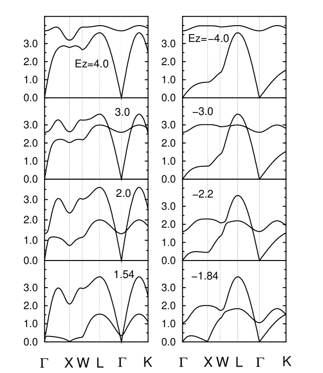
Figure 21: Spin-wave and spin-and-orbital-wave excitations in the G-AF phases: AFxx (left) and AFzz (right), in the main directions of the 3D BZ for a few values of $E_{z}$ (in the units of $J$), and for $J_{H}/U=0.3$. The lower-energy mode becomes soft for $E_{z}/J<1.54$ ($E_{z}/J>-1.84$) in the AFxx (AFzz) phase. To allow a direct comparison, both phases are shown using the 3D BZ for a $bcc$ lattice with the standard notation of high symmetry points: $\Gamma=(0,0,0)$, $X=(\pi,0,0)$, $W=(\pi,\pi/2,0)$, $L=(\pi/2,\pi/2,\pi/2)$ and $K=(3\pi/4,3\pi/4,0)$ (after Ref. Ole00 ).

For that purpose, let us introduce here the local operators constituting the $so(4)$ Lie algebra at site $i$ as Hubbard operators, $X_{i}^{\alpha\beta}=|i\alpha\rangle\langle i\beta|$. Using the unity operator, $\sum_{\beta}X_{i}^{\beta\beta}={\cal{I}}$, the diagonal operator $X_{i}^{\alpha\beta}$ that refers to the state $|i\alpha\rangle$ realized at site $i$ in the classical ground state of the phase under consideration may be expanded in terms of the excitation operators,

$$X_{i}^{\alpha\alpha}={\cal{I}}-\sum_{\beta\neq\alpha}X_{i}^{\beta\alpha}X_{i}^{\alpha\beta},$$ (132)

while the diagonal operators referring to excited states $|i\beta\rangle$ are expressed as

$$X_{i}^{\beta\beta}=X_{i}^{\beta\alpha}X_{i}^{\alpha\beta}.$$ (133)

Applying these equations to the $z$-th spin component $S^{z}_{i}=S^{z}_{ixx}+S^{z}_{izz}$ of the total spin at site $i$ in one of the G-AF phases with pure orbital character (say AFxx for definiteness), one finds, for $i$ in the spin-up sublattice Ole00 ,

$$S_{i}^{z} = \frac{1}{2}(X_{i}^{x\uparrow,x\uparrow}-X_{i}^{x\downarrow,x\downarrow}+X_{i}^{z\uparrow,z\uparrow}-X_{i}^{z\downarrow,z\downarrow})$$ (134)

$$= \frac{1}{2}{\cal{I}}-X_{i}^{x\downarrow,x\uparrow}X_{i}^{x\uparrow,x\downarrow}-X_{i}^{z\downarrow,x\uparrow}X_{i}^{x\uparrow,z\downarrow}=\frac{1}{2}{\cal{I}}-S_{ixx}^{-}S_{ixx}^{+}-K_{izx}^{-}K_{ixz}^{+}.$$

Taking the average of Eq. (134) one obtains, with the MF value $\langle S_{i}^{z}\rangle_{\rm MF}=\frac{1}{2}$,

$$\langle S_{i}^{z}\rangle_{\rm RPA}=\frac{1}{2}-\langle S_{i}^{-}S_{i}^{+}\rangle-\langle K_{i}^{-}K_{i}^{+}\rangle=\langle S_{i}^{z}\rangle-\delta\langle S_{i}^{z}\rangle,$$ (135)

where the averages like $\langle S_{ixx}^{-}S_{izz}^{+}\rangle$ are zero since they involve ‘ghost’ modes, so that one may formally replace $S_{ixx}^{+}$ by $S_{ixx}^{+}+S_{izz}^{+}=S_{i}^{+}$, etcetera. The first contribution $\propto\langle S_{i}^{-}S_{i}^{+}\rangle$ is the usual renormalization due to spin waves, while the second term $\propto\langle K_{i}^{-}K_{i}^{+}\rangle$ stands for the reduction of $\langle S_{i}^{z}\rangle_{\rm RPA}$ due to spin-and-orbital excitations. Both terms involve a local excitation preceded by a deexcitation which reproduces the initial local state. As expected, only transverse excitations contribute to the spin renormalization. Note that, since Eq. (134) is an exact operator relation, the present procedure guarantees that Eq. (135) is a conserving approximation which respects the sum rule for the occupancies of all states, $\sum_{\beta}\langle X_{i}^{\beta\beta}\rangle=1$. The generalization of Eq. (135) to the MO phases using the operators ${\cal S}_{i}^{\pm}$ and ${\cal K}_{i}^{\pm}$ in the expansion of ${\cal S}_{i}^{z}$, or to other order parameters, like the orbital polarization (86), is straightforward.

The local correlation functions which renormalize the order parameter in Eq. (132) are determined in the standard way Hal72 ,

$$\langle B_{i}^{\dagger}A_{i}\rangle=\frac{1}{N}\sum_{\vec{k}}\int_{-\infty}^{+\infty}d\omega{\cal A}_{AB^{\dagger}}({\vec{k}},\omega)\frac{1}{\exp(\beta\omega)-1},$$ (136)

where $\beta=1/k_{B}T$, and

$${\cal A}_{AB^{\dagger}}({\vec{k}},\omega<0)=2{\rm Im}\langle\langle A_{\vec{k}}|B^{\dagger}_{\vec{k}}\rangle\rangle_{\omega-i\epsilon}=\sum_{\nu<0}{\cal A}_{AB^{\dagger}}^{(\nu)}({\vec{k}})\delta(\omega-\omega_{\vec{k}}^{(\nu)})$$ (137)

is the respective spectral density for the negative frequencies ($\nu<0$), and ${\cal A}_{AB^{\dagger}}^{(\nu)}({\vec{k}})$ are the respective spectral weights. Therefore, the correlation functions at $T=0$ are found by summing up the total spectral weight at the negative frequencies,

$$\langle B_{i}^{\dagger}A_{i}\rangle=\frac{1}{N}\sum_{\vec{k}}\sum_{\nu<0}{\cal A}_{AB^{\dagger}}^{(\nu)}({\vec{k}}).$$ (138)

Before discussing the renormalization of the order parameter and the corresponding energies in RPA, we concentrate ourselves on the behavior of the transverse excitations when the crossover lines between the classical phases are approached. As already emphasized in Sec. III.C, the spin-wave and spin-and-orbital-wave excitations couple. As a consequence, the modes in all considered phases soften when the transition lines between different classical phases, or classical degeneracy point are approached. This softening is shown for a representative value of $J_{H}/U=0.3$ in Fig. 21 for the two AF phases with either $|x\rangle$ or $|z\rangle$ orbitals occupied. In the AFxx phase the energy scales of both excitations are separated for $E_{z}>4J$, while the spin-and-orbital mode moves towards zero energy with decreasing $E_{z}$, and finally becomes soft at the $X$ point, along $\vec{k}=(\pi,0,k_{z})$ and along equivalent lines in the BZ for $E_{z}\simeq 1.54J$. A similar mode softening is found for the AFzz phase at $E_{z}<0$, with the soft mode along $\Gamma-X$ and equivalent directions in the BZ at $E_{z}\simeq-1.84J$. This peculiar softening along lines and not at points in the BZ shows that the modes behave 2D-like instead of 3D-like: constant-frequency surfaces are cylinders contracting towards lines, not spheres contracting towards a point.

By making an expansion of Eq. (103) around the soft-mode lines, one finds that the (positive) excitation energies are characterized by finite masses in the perpendicular directions:

$$\omega_{\rm AFxx}(\vec{k})\rightarrow\Delta_{x}+B_{x}\left({\bar{k}}_{x}^{4}+14{\bar{k}}_{x}^{2}k_{y}^{2}+k_{y}^{4}\right)^{1/2},$$ (139)

independently of $k_{z}$ (here ${\bar{k}}_{x}=k_{x}-\pi$) for the AFxx phase, and

$$\omega_{\rm AFzz}(\vec{k})\rightarrow\Delta_{z}+B_{z}\left(k_{y}^{2}+4k_{z}^{2}\right),$$ (140)

independently of $k_{x}$, and similarly along the $\Gamma-Y$ direction with $k_{y}$ replaced by $k_{x}$ for the AFzz phase. As an example we give explicit expressions for the AFxx phase at $\eta=0$,

$$\Delta_{x}=\frac{9}{2}\frac{\varepsilon_{z}}{\varepsilon_{z}+3},\hskip 34.14322ptB_{x}=\frac{27}{16}\frac{1}{\varepsilon_{z}+3},$$ (141)

where one finds that the gap $\Delta_{x}\to 0$ when $\varepsilon_{z}\to 0$, i.e., upon approaching the $M=(E_{z},J_{H})=(0,0)$ point at which the AF order is changed to the AFzz phase. This illustrates a general principle: $\Delta_{i}\to 0$ when the crossover line to another phase is approached, and $B_{i}\neq 0$ when the modes (139) and (140) soften, making quantum fluctuation corrections to the order parameter to diverge logarithmically, $\langle\delta S\rangle\sim\int d^{3}k/\omega(\vec{k})\sim\int d^{2}k/(\Delta_{i}+B_{i}k^{2})\sim\ln\Delta_{i}$. We emphasize that for the occurrence of this divergence not only the finiteness of the mass, but also the 2D-like nature of the dispersion is essential. It enables a 3D system to destabilize LRO by what are essentially 2D fluctuations. So the divergence of the order parameter near the crossover lines in the phase diagram and the associated instability of the classical phases, may be regarded as another manifestation of the effective reduction of the dimensionality occurring in the spin-orbital model. We do not present explicitly the softening of the longitudinal modes which also happens at the transition lines, but has no direct relation to the stability of classical phases.

Figure 22: The same as in Fig. 21, but for decoupled spin-wave and spin-and-orbital-wave excitations in the G-AF phases (after Ref. Ole00 ).

A seemingly attractive way to simplify the calculation of the transverse excitations would be to make a decoupling of the spin-waves and spin-and-orbital-waves. However, this is equivalent to violating the commutation rules between the spin and spin-and-orbital operators Fei98 , and this changes the physics. It gives the same excitation energies as Eq. (103), but with $P_{\alpha\vec{k}}=0$; the numerical result is given in Fig. 22. Of course, the spin-wave excitation does not depend then on the orbital splitting $E_{z}$, and the spin-and-orbital-wave excitation gradually approaches the line $\omega_{\vec{k}}=0$ with decreasing $|E_{z}|$. It has a weak dispersion which depends on $J_{H}$ and on the value of $|E_{z}|$, and gives an instability at the $\Gamma$ point only, not at certain lines in the BZ. The instability occurs well beyond the transition lines in the phase diagram of Fig. 12, i.e., within the MOFFA and MOAFF phase for $E_{z}<0$ and $E_{z}>0$, respectively. Such spin-wave and spin-and-orbital-wave modes give, of course, much smaller quantum corrections of the order parameter and energy than the correct RPA spectra of Fig. 21 Fei98 ; Ole00 .

Figure 23: Transverse (full lines) and longitudinal (dashed lines) excitations in MOFFA phase in the main directions of the 3D BZ for a few values of $J_{H}/U$, and for $E_{z}/J=-0.5$. The lower-energy mode becomes soft for $J_{H}/U<0.06$ (after Ref. Ole00 ).

The spin waves in the MOFFA phase, stable at $E_{z}<0$, soften with decreasing $\eta$ (53), as shown in Fig. 23. At large $\eta$ the spin-and-orbital waves at high energies are well separated from the spin-wave modes. The latter have a rather small dispersion at $J_{H}/U=0.3$ which follows from relatively weak FM interactions in the $(a,b)$ planes, and AF interactions along the $c$-axis. The modes start to mix stronger with decreasing $\eta$, and finally the gap in the spectrum closes below $\eta=0.1$. The mode softening occurs again along lines in the BZ, namely along the $\Gamma-X$ direction. Unfortunately, an analogous analytic expansion of the energies near the softening point to those in the AFxx and AFzz phases could not be performed, but the reported numerical results suggest a qualitatively similar behavior to these two phases. The MOAFF phase gives an analogous instability for $E_{z}>0$.

The soft modes in the excitation spectra give a very strong renormalization of the order parameter $\langle S^{z}\rangle_{\rm RPA}$ in RPA (135) near the mode softening, as shown in Fig. 24. The quantum corrections exceed the MF values of the order parameter in the AFxx and AFzz phases in a region which separates these two types of LRO. Although one might expect that another classical phase with mixed orbitals and FM planes sets in instead, and the actual instabilities where $\delta\langle S_{z}\rangle\to\infty$ are found indeed beyond the transition lines to another phase, the lines where $\delta\langle S^{z}\rangle=\langle S^{z}\rangle$ occur still before the phase boundaries in the phase diagram of Fig. 12 (see Fig. 1 of Ref. Fei97, ). This leaves a window where no classical order is stable in between the G-AF and A-AF spin structures.

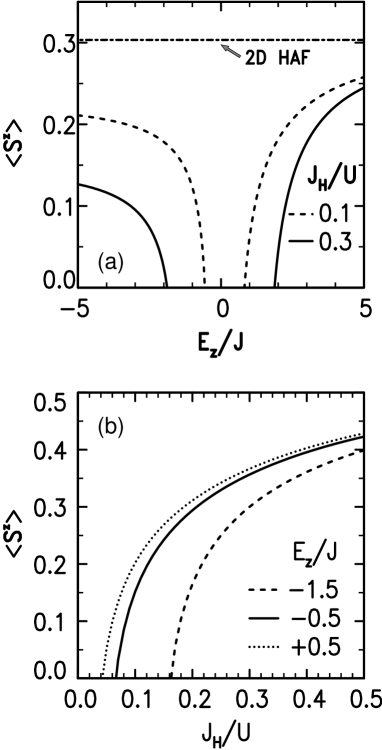
Figure 24: Renormalization of the magnetic LRO parameter $\langle S^{z}_{i}\rangle$ by quantum fluctuations as obtained in RPA in: (a) AFzz (left) and AFxx (right) phases as functions of $E_{z}/J$ for $J_{H}/U=0.1$ and $0.3$; (b) MOFFA phase as function of $J_{H}/U$ for $E_{z}/J=0.5$, -0.5 and -1.5 (after Ref. Ole00 ).

The origin of such a strong renormalization of $\langle S^{z}\rangle$ may be better understood by decomposing the quantum corrections into individual contributions as given in Eq. (135). The leading correction comes from the local spin fluctuation expressed by $\langle S^{-}_{i}S^{+}_{i}\rangle$ and enhanced with respect to the pure spin model, while the spin-and-orbital fluctuation, $\langle K^{-}_{i}K^{+}_{i}\rangle$, increases rapidly when the instability lines $\langle S^{z}\rangle_{\rm RPA}=0$ are approached. Interestingly, the latter fluctuation is stronger in the AFxx than in the AFzz phase for the same values of $J_{H}$ and $|E_{z}|$ which demonstrates that the AFzz phase is more robust due to the directionality of the $|z\rangle$ orbitals and the strong AF bonds along the $c$-axis. This asymmetry is also visible in Fig. 24, where $\langle S^{z}\rangle_{\rm RPA}$ decreases somewhat faster towards zero for $E_{z}>0$.

In both G-AF phases (AFxx and AFzz) the leading contribution to the renormalization of $\langle S^{z}\rangle_{\rm RPA}$ comes from the lower-energy mode, especially at larger values of $J_{H}$. In the case of $J_{H}=0$ one finds, however, that the contribution from the lower mode either stays approximately constant (in the AFxx phase), or even decreases (in the AFzz phase) when the line of the collapsing LRO is approached at $|E_{z}|\to 0$. This latter behavior shows again that the coupling between the spin-wave and spin-and-orbital-wave excitations is of crucial importance Fei98 . This is further illustrated by Fig. 25, which shows the renormalization of $\langle S_{z}\rangle$ as obtained when spin waves and spin-and-orbital waves are decoupled in the manner discussed above. One observes that significant reduction of $\langle S_{z}\rangle$ then sets in only very close to the actual divergence.

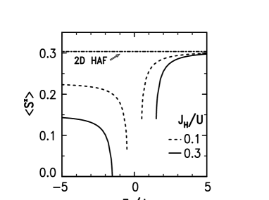
Figure 25: Renormalization of the magnetic LRO parameter $\langle S^{z}_{i}\rangle$ by quantum fluctuations as obtained in RPA in: (a) AFzz (left) and AFxx (right) phases as functions of $E_{z}/J$ for $J_{H}/U=0.1$ (dashed lines) and $0.3$ (solid lines); (b) MOFFA phase as functions of $J_{H}/U$ for $E_{z}/J=0.5$, -0.5 and -1.5 (after Ref. Ole00 ).

The reduction of $\langle S^{z}\rangle_{\rm RPA}$ in the MOFFA/MOAFF phases, described by a relation similar to Eq. (135), is in general weaker than that in the G-AF phases. This is understandable, as the quantum fluctuations contribute here only from a single AF direction, while the FM order in the planes does not allow for excitations which involve spin flips and stabilizes the LRO of A-AF type. For fixed $J_{H}$ one finds increasing quantum corrections $\delta\langle S^{z}\rangle$ when the lines of phase transitions towards the AF phases are approached. These corrections increase faster with increasing $|E_{z}|$ in the MOFFA phase, as the increasing occupancy of the $|z\rangle$-orbital makes the AF interaction stronger there than in the MOAFF phase, where the occupancy of the $|x\rangle$ orbital increases slower roughly by a factor of two. It may be again concluded Ole00 that the collapse of the LRO in the A-AF (MO) phases is primarily due to increasing spin fluctuations, $\langle{\cal S}^{-}_{i}{\cal S}^{+}_{i}\rangle$, while the spin-and-orbital $\langle{\cal K}^{-}_{i}{\cal K}^{+}_{i}\rangle$ fluctuations become of equal importance only when the multicritical point of the Kugel-Khomskii model $M=(E_{z},J_{H})=(0,0)$ is approached.

The orbital polarization (86) is also renormalized by the quantum fluctuations, but this is a rather mild effect not showing any instability (Fig. 26). In fact, this renormalization involves only the spin-and-orbital and the orbital excitation but not the spin excitation, which gives the largest weight in the lowest transverse mode that goes soft. The value determined in RPA is calculated from an expression similar to Eq. (135), e.g. in the AFxx phase from

$$\langle n_{ix}\rangle_{\rm RPA}=1-4\,\langle T_{izx}T_{ixz}\rangle-\langle K^{-}_{i}K^{+}_{i}\rangle.$$ (142)

The density $\langle n_{ix}\rangle_{\rm RPA}$ decreases gradually with decreasing $E_{z}$, with somewhat increased quantum corrections close to the transition lines between different classical phases. In the MOAFF phase one finds nonequivalent sublattices, with enhanced/reduced $\langle n_{ix}\rangle_{\rm RPA}$ from its average value, reflecting the shape of the occupied orbital on a given sublattice.

Figure 26: Average density of $|x\rangle$-holes $\langle n_{x}\rangle$ as obtained in RPA for $J_{H}/U=0.3$ in MF approximation (dashed lines) and with the quantum corrections calculated in RPA (full lines). The splitting of lines for $E_{z}/J>0$ corresponds to the MOAFF phase with two different hole densities $\langle n_{x}\rangle_{A}\neq\langle n_{x}\rangle_{B}$ on the ions belonging to two sublattices shown in Fig. 11 (after Ref. Ole00 ).

Finally, we note that the dominating contribution to the quantum corrections to the energy comes from the transverse excitations. The longitudinal excitations do not contribute at all at $J_{H}/U=0$, where these modes are dispersionless. Otherwise, the orbital excitations have always a significantly smaller dispersion than the value of the orbital gap in the spectrum, and the resulting quantum corrections are therefore almost negligible.

Summarizing, we have reported the case that a generic (Kugel-Khomskii) model for the dynamics of an orbitally degenerate MHI is characterized by a number of peculiar features. Assuming that the ground state exhibits some particular classical spin- and orbital order, the stability of this order can be investigated by considering the Gaussian fluctuations around this state. In this way we find that in various regimes of the zero-temperature phase-diagram, classical order is defeated by the quantum fluctuations, and we expect a qualitative phase diagram with a region of disordered phases Fei97 . These disordered phases with short-range spin and orbital correlations are discussed in the next Section.

IV.3 Spin disorder: VB and RVB states

Generally speaking, the ground state is unknown for most systems described by the Heisenberg model with nonferromagnetic interactions. Even those that are known in analytical form, such as the Bethe solution in one dimension Bet31 , require numerical computations to determine the spin correlations. Under these circumstances, variational wave functions can give good guesses for the ground state. In this respect, the valence bond (VB) states and/or plaquettes valence bond (PVB) states are variational wave functions which play a prominent role in approximating the leading spin-spin correlations for the AF Heisenberg model. They have been studied largely in the context of quantum magnetism, especially in recent years when new motivation occurred due to the research aimed at a better understanding of the magnetic states realized in high temperature superconductors.

Their general form can be written in the following way Faz99 ; Aue94 :

$$|c_{\alpha},S\rangle=\sum_{\alpha}c_{\alpha}|\alpha\rangle,$$ (143)

where $c_{\alpha}$ are variational parameters and

$$|\alpha\rangle=\prod_{\langle ij\rangle\epsilon\Lambda_{\alpha}}(a^{\dagger}_{i}b^{\dagger}_{j}-b^{\dagger}_{i}a^{\dagger}_{j})|0\rangle,$$ (144)

with $a_{i}$ and $b_{i}$ being the Schwinger bosons on site $i$ Aue94 . $\Lambda_{\alpha}$ is a particular configuration of bonds $\langle ij\rangle$ which cover the whole lattice and are occupied by spin singlets. The essence of a VB state is that there are no magnetic correlations between different singlets. The condition on $\Lambda_{\alpha}$ is that precisely $2S$ bonds will emanate from each site. In some cases there will be only few configurations to contribute in the large lattice limit. The case were there are macroscopically many configurations and VB states resonate between them has been called resonating valence bond (RVB) states and was introduced by Anderson And87 . Considering the expression given in Eq. (143), it is easy to verify that all bond operators are invariant under SU(2) transformations. Therefore, the VB wave function $|c_{\alpha},S\rangle$ is a singlet in the total spin. It provides an example of spin-disordered state, the so-called spin liquid.

There exists a class of special Hamiltonians for which the VB states are the exact ground states. Majumdar and Ghosh introduced the Hamiltonian for spin $S=1/2$ Maj69 :

$$H_{\rm MG}=\frac{4K}{3}\sum_{i=1}^{N}\left({\vec{S}}_{i}\cdot{\vec{S}}_{i+1}+\frac{1}{2}{\vec{S}}_{i}\cdot{\vec{S}}_{i+2}\right)+\frac{1}{2}N,$$ (145)

where $i$ stands for the sites of a 1D chain with an even number of sites $N$, $K>0$ and one assumes periodic boundary conditions, with ${\vec{S}}_{N+1}={\vec{S}}_{1}$ and ${\vec{S}}_{N+2}={\vec{S}}_{2}$. It is straightforward to show that the dimer state,

$$|d\rangle_{\pm}=\prod_{n=1}^{N/2}\left(|\uparrow_{2n}\rangle|\downarrow_{2n\pm 1}\rangle-|\downarrow_{2n}\rangle|\uparrow_{2n\pm 1}\rangle\right)/\sqrt{2},$$ (146)

has energy zero, that is $H_{\rm MG}|d\rangle_{\pm}=0$, and all the other eigenenergies are positive. As one can see the Hamiltonian $H_{\rm MG}$ includes AF interactions between next-nearest neighbors which frustrates the nearest neighbor correlations. Thus, one expects the ground state to be more disordered than that in the usual Heisenberg model. Indeed, for the antiferromagnet with only nearest neighbor interactions the spin-spin correlations decay as an inverse of a power of distance, while the wave function $|d\rangle_{\pm}$ has state dimer correlations that is they vanish beyond the nearest neighbors. The proof is interesting since it provides a method for constructing a more general family of Hamiltonians whose ground states are VB states Aue94 .

The basic idea is to express $H_{MG}$ in terms of projection operators. If we consider three spins $S=1/2$ on an arbitrary triad of sites, the total spin $J$ may be either equal to $3/2$ or to $1/2$. The total spin of three sites $(i-1,i,i+1)$ is given by

$${\vec{J}}_{i}={\vec{S}}_{i-1}+{\vec{S}}_{i}+{\vec{S}}_{i+1}$$ (147)

and its square is connected to the $H_{MG}$ via the projection operator on a configuration of spin $1/2$ on three sites in the following way:

$$Q_{3/2}(i-1,i,i+1) = \frac{1}{3}\left(J_{i}^{2}-\frac{3}{4}\right)=\frac{1}{2}+\frac{2}{3}\left({\vec{S}}_{i}\cdot{\vec{S}}_{i-1}+{\vec{S}}_{i-1}\cdot{\vec{S}}_{i+1}+{\vec{S}}_{i}\cdot{\vec{S}}_{i+1}\right),$$ (148)

so that the Hamiltonian can be rewritten as

$$H_{\rm MG}=K\sum_{i}Q_{3/2}(i-1,i,i+1).$$ (149)

Of course, $Q_{3/2}(i-1,i,i+1)$ annihilates any state with $J=1/2$ at the three sites $\{i-1,i,i+1\}$. Since the dimer states $|d\rangle_{\pm}$ (146) do not contain states with total $J_{z}>1/2$ on any three sites and due to the rotational invariance of the state $|d\rangle_{\pm}$ there cannot be any $J>1/2$ component in it. Therefore, each operator $Q_{3/2}(i-1,i,i+1)$ annihilates $|d\rangle_{\pm}$. Moreover, since the $Q_{3/2}(i-1,i,i+1)$ have only positive eigenvalues, $|d\rangle_{\pm}$ is the ground state of $H_{\rm MG}$.

In a similar fashion Affleck, Kennedy, Lieb, and Tasaki Aff87 have constructed the Hamiltonians for the VB solids as ground states which cover the whole lattice,

$$H_{\rm AKLT}=\sum_{\langle ij\rangle}\sum_{J=2S-M+1}^{2S}K_{J}Q_{J}(ij),$$ (150)

where the bond projector $Q_{J}(ij)$ projects the total bond spin of magnitude $J$. In this case it can be proven as before, that the ground state is

$$|\Omega_{\rm VBS}\rangle=\prod_{\langle ij\rangle}\left(a^{\dagger}_{i}b^{\dagger}_{j}-b^{\dagger}_{i}a^{\dagger}_{j}\right)^{M}|0\rangle,$$ (151)

where all the nearest neighbor bonds $\langle ij\rangle$ are included in the product, and $M=2S/z$ is an integer which is related to the spin $S$ and to the coordination number $z$ of the considered lattice. By construction, the smallest $S$ which allows to construct such states is $S=1$ for a 1D lattice.

Spontaneous spin liquid states occur in 2D lattices due to frustrating spin interactions. The basic model which shows such a behavior is the 2D AF $J_{1}-J_{2}$ Heisenberg model on a square lattice Cha88 ; Cha88a ; Cha88b ; Cha88c ; Cha88d ; Chu91 . There are two main reasons why this model holds a special place in the physics of spin systems. It is one of the simplest models which exhibits quantum transitions between long-range ordered phases and a quantum disordered phase – a topic of fundamental interest Sac99 . Moreover, even though the $J_{1}-J_{2}$ model (Fig. 27) does not deal with charge dynamics, it can represent a good starting point for the understanding of how translational symmetry is broken in a purely insulating spin background for approaching this question in spin systems with finite doping. The $J_{1}-J_{2}$ model has been discussed in numerous works over the last ten years and some of the important issues that have been addressed are: (i) how is the Néel order, present for small frustration ($J_{2}$), destroyed as frustration increases, and (ii) is a quantum disordered phase present in a finite window of frustration, and what is the structure of this phase?

Figure 27: Disordered magnetic states for a 2D square lattice with AF interactions $J_{1}$ and $J_{2}$: (a) plaquette-RVB, and (b) columnar (VB) dimer ground states. The bold lines indicate the bonds occupied by spin singlets.

Spin-wave calculations, both at the non-interacting level as well as including interactions perturbatively in powers of $1/S$ ($S$ is the spin value), have found that the magnetization decreases with increasing frustration, ultimately vanishing at a critical value Iga93 . These calculations however cannot predict the structure of the phase beyond the instability point, or the location of the phase boundary with high accuracy, since as the magnetization decreases more and more powers of $1/S$ have to be included (strong spin-wave interactions). Exact diagonalization (ED) of clusters as large as $N=36$ Sch94 ; Sch96 have found a finite region of quantum disordered (gaped) phase, but have failed to determine accurately the dominant short-range correlations or type of order (e.g. dimer, plaquette, etcetera) characterize this phase. The ED calculations also suffer from large finite-size corrections, especially for strong frustration. An insight into the structure of the disordered phase was possible with the help of the large $N$ expansion technique Sac90 ; Cha88b . These authors predicted the quantum disordered phase to be spontaneously dimerized in a particular (columnar) configuration (Fig. 27). High order dimer series expansions around this configuration were performed Gel89 ; Kot99 , all confirming its stability in a window of frustration. Thus the spontaneously dimerized state has emerged as the most probable candidate for a disordered ground state. Let us mention in this connection that in 1D systems the Lieb-Schultz-Mattis (LSM) theorem guarantees that a gaped phase in a quantum spin system breaks translational symmetry Lieb61 . Extension of the LSM theorem to two-dimensions was proposed Aff88 but not yet proven in the most general case. The large $N$ and dimer series results, however, seem to confirm the validity of the LSM theorem in two dimensions as well, including, in fact, the case of finite doping Sac99a .

The previous case is a classical example that inclusion of additional interactions, such as dimerization and/or frustration, leads to increased quantum fluctuations, and ultimately to vanishing LRO at a critical coupling. In this context, further examples of transitions caused by local alternation of the exchange couplings are the dimerized Heisenberg antiferromagnets Kat93 , the two-layer Heisenberg model Mil94 ; San94 ; Chu95 and the CaV₄O₉ lattice (1/5- depleted square lattice) Ued96 ; Ued96a ; Tro96 ; Whi96 . For these situations, the local dimer or plaquette correlations eventually win over the long-range Néel order, leading to a disordered ground state.

An important issue concerning the quantum transitions mentioned above is their universality class. It is generally accepted that the effective low-energy theory for the 2D Heisenberg systems with a collinear (Néel) order parameter is the O(3) non-linear sigma model (NLSM) in 2+1 dimensions Fra91 . This field theory contains a single effective coupling constant $g$ and, at $T=0$, describes the ordered Néel phase for $g<g_{c}$. For $g>g_{c}$ the NLSM is in a quantum disordered phase with a finite correlation length. However the determination of $g_{c}$ and the nature of the disordered phase are beyond the field theory formulation and depend on the specific details of the model. In addition, Berry phases associated with instanton tunneling between topologically different configurations are present in the NLSM Hal88 . In one dimension the Berry phase effects are known to be important, essentially leading to the difference between the excitations in the integer and half odd-integer spin chains Aff88 (Haldane conjecture). In two dimensions Berry phases are also present, but their role is less clear. If one neglects these purely quantum effects, the universality class of the quantum transitions in the 2D Heisenberg antiferromagnet should be the same as that of the classical O(3) vector model in three dimensions. QMC simulations performed on the two-layer antiferromagnet Sand95 , and on the CaV₄O₉ lattice Tro96 confirm with high accuracy that the quantum transitions in the above two models happen in the O(3) universality class.

Furthermore, the $J_{1}-J_{2}$ model, which exhibits a quantum transition due to frustration, could represent a case of difference from the O(3) universality class. Read and Sachdev showed that there are two correlation lengths close to the criticality Cha88b , suggesting to think that there are deviations in the universality class. On the other hand, they showed that only one of the two is relevant implying that even though the Berry phases are relevant in the disordered phase, ultimately, near the critical point, their effect disappears.

As we have discussed, the main characters in this topic are low-dimensional quantum spin systems (spin chains Whi94 and ladders Dag96 ; Dag96a ; Dag96b ), and it proves difficult to achieve quantum melting of magnetic LRO in empirically relevant systems in higher dimensions. It is therefore worth pointing out that there is a class of systems in which quantum-melting occurs due to a unique mechanism which operates in three dimensions: small spin, orbital degenerate MHI, the so-called Kugel-Khomskii systems Kug82 . There might exist already a physical realization of such a 3D quantum spin-orbital liquid: spin disorder in LiNiO₂Hir85 ; Hir85a .

Here, we report how the orbital degeneracy operates through the same basic mechanisms known from spin systems, to produce quantum melting in the spin-orbital $d^{9}$ systems. The novelty is that these systems tend to ”self-tune” to (critical) points of high classical degeneracy. There are interactions which may lift the classical degeneracy, but they are usually weak. An interaction of this kind is the electron-phonon coupling – the degeneracy is lifted by a change in crystal structure, the conventional collective JT instability. As we have discussed in Sec. III.C, the lattice has to react to the symmetry lowering in the orbital sector, but it was recently convincingly shown, at least in the archetypical compound KCuF₃, that the structural distortion is a side effect Lie95 . The fundamental question which arises in this context is what happens when the classical order becomes unstable against quantum fluctuations. Although the subject is much more general (singlet-triplet models in rare earth compounds Hsi72 , V₂O₃ Cas78 , LaMnO₃ Miz96 , heavy fermions Ful91 ; Faz99 ; Cox87 ), we focus here on the simplest situation encountered in KCuF₃ and related systems, described by the $d^{9}$ model Fei97 .

If the classical limit is as sick as explained in Sec. IV.B, what is happening instead? A priori it is not easy to give an answer to this question. There are no ‘off the shelf’ methods to treat quantum spin problems characterized by classical frustration, and the situation is similar to what is found in, e.g. $J_{1}-J_{2}-J_{3}$ problems Cha88 ; Cha88a ; Cha88b ; Cha88c ; Cha88d . A first possibility is quantum order-out-of-disorder Chu91 : quantum fluctuations can stabilize a particular classical state over other classically degenerate states, if this particular state is characterized by softer excitations than any of the other candidates. Khaliullin and Oudovenko Kha97 have suggested that this mechanism is operative in the present spin-orbital model, where the 3D anisotropic AFzz antiferromagnet is the one becoming stable. Their original argument was flawed because of the decoupling procedure they used which violates the so(4) dynamical algebra constraints Fei98 . Nevertheless, there is yet another possibility: VB singlet (or spin-Peierls) order, which at the least appears in a more natural way in the present context than is the case of higher dimensional spin-only problems, because it is favored by the directional nature of the orbitals.

In similarity to the purely spin systems, in the presence of orbital interactions either one particular covering of the lattice with these ‘spin-dimers’ might be favored (VB or spin-Peierls state), or the ground state might become a coherent superposition of many of such coverings (RVB state). On a cubic lattice the difficulty is that although much energy is gained in the formation of the singlet pairs, the bonds between the singlets are treated poorly. Nevertheless, both in 1D spin systems (Majumdar-Ghosh Maj69 , AKLT-systems Aff87 ) and in the large $N$ limit of $SU(N)$ magnets in two dimensions Sac99 , ground states are found characterized by spin-Peierls/VB order Cha88b .

Figure 28: A variety of VB (VBa and VBc) and PVB (PVBA and PVBIc) solids discussed in the text for the $d^{9}$ model (after Ref. Zaa99 ).

In principle, various topologically different coverings of the 3D lattice may be considered, in analogy with the square lattice Kiv87 . Two obvious choices, defined by the sets $\Lambda_{\alpha}$ of parallel singlets in Eq. (144), and suggested by the tendency towards particular directional orbitals for positive (negative) $E_{z}$ are: ($i$) singlets along the $a$-axis with orbitals close to $3x^{2}-1$ (VBa), expected to be favored for $E_{z}>0$, and ($ii$) singlets along the $c$-axis with orbitals $\sim|z\rangle$ (VBc), preferred if $E_{z}<0$ (see Fig. 28). Interestingly, the immanent frustration of the magnetic interactions in the spin-orbital model (57) causes that these phases have lower energies than the classical phases in a broad parameter regime. This result is already quite spectacular when one realizes that such VB phases thus appear to be better approximations to the exact ground state than the classical phases with magnetic LRO in three dimensions. An example is shown in Fig. 29 for $J_{H}/U=0.2$; as expected, VBa (VBc) has a lower energy for $E_{z}>0$ ($E_{z}<0$), and both phases are degenerate at $E_{z}=0$. We have recognized that the exceptional stability of these (nonresonating) VB states is due to a unique mechanism involving the orbital sector. Unlike in the spin system with a simple Heisenberg exchange, the bonds not occupied by the singlets contribute orbital energy and this is optimized when singlets in orthogonal directions are connected (which is not the case in the VBa and VBc phases; see further below).

Figure 29: Energies of the various ordered and disordered phases for the $d^{9}$ model (57)–(59) as functions of $E_{z}/J$, for $J_{H}/U=0.2$. The energies of classical phases were calculated within MF (short-dashed lines) and RPA approach (full lines), while the energies of VBa and VBc states (see Fig. 28) are given by dashed-dotted lines. The energies of disordered states (RVBc, PVBI, and PVBA) stable close to the orbital degeneracy are given by the long-dashed lines (after Ref. Foz00 ).

Further improvement of energy may be expected by including the leading quantum fluctuations in the VB (VBa and VBc) states. In the case of the VBa phase this leads directly to constructing the PRVB states, with the plaquette wave functions of the type,

$$|\Psi_{\Box}\rangle={1\over\sqrt{2|1+S|}}(|\Psi_{a}\rangle+e^{i\phi}|\Psi_{b}\rangle),$$ (152)

where the two components are composed of the singlet pairs along $a$ and $b$-axis, $|\Psi_{a}\rangle$ and $|\Psi_{b}\rangle$, respectively, and $S=e^{i\phi}\langle\Psi_{a}|\Psi_{b}\rangle$ is the overlap. It is straightforward to show that this Ansatz gives an exact energy $E_{0}=-2J_{0}$ for a plaquette occupied by spins $S=1/2$, assuming the AF interaction $J_{0}$. The wave function $|\Psi_{\Box}\rangle$ turns out to be identical with the exact wave function of an isolated plaquette Isk87 , if we make the choice $\phi=0$ in Eq. (152). When averaged over the square lattice, this gives an energy of $-J_{0}/2$ per site, the same energy as that of the classical Néel state. However, in the present case the resonance between the two singlet structures is much weaker, as the optimized orbitals are either $\parallel a$, or $\parallel b$ in the two components of the plaquette wave function (152). This results in a much smaller overlap $S=1/32$ and typically very small offdiagonal energy elements, $\langle\Psi_{a}|H|\Psi_{b}\rangle$. As a result, the improvement due to this resonance is marginal, and it turns out to be better to optimize the singlet distribution over the lattice with respect to the energy contributions which originate from the bonds not occupied by the singlets.

There are three different possible energy contributions for these bonds depending on whether they connect: ($i$) two singlets along a single ($a$, $b$, or $c$) line, ($ii$) two singlets oriented along two different lines with an angle of $\pi/2$, or ($iii$) two parallel singlets, with the bond making itself an angle of $\pi/2$ to both of them. As the second type of the non-singlet bonds is energetically the most favorable, more energy than in the PRVB state (152) is gained if the plaquette wave functions $|\Psi_{a}\rangle$ and $|\Psi_{b}\rangle$ alternate and form a superlattice (see Fig. 30). This results in a plaquette VB (PVB) state for each $(a,b)$ plane. As also the energy of the vertical ($\parallel c$) bonds is optimized when these bonds connect one singlet $\parallel a$ and another $\parallel b$, the optimal phase with a lower energy that the quantum-corrected MOAFF phase found for $E_{z}>0$ (Fig. 29) is given by a PVB alternating (PVBA) state, with the alternation of two along the $c$-axis (see Figs. 28 and 30). We note that the energy comparison between the AFxx state and the PVBA state resembles qualitatively the situation in a 2D 1/5-depleted lattice Ued96 ; Ued96a , but the spin-disordered state is remarkably more stable in our case, and provides an approximate Ansatz for the ground state in three dimensions.

Figure 30: Schematic representation of the PVBA state, stable in a range of $J_{H}/U$ and for $E_{z}/J>0$. The open and full circles refer to the directional $|\zeta\rangle$ orbitals parallel to the bonds occupied by the singlets along $a$ and $b$ axis, respectively (after Ref. Foz00 ).

In contrast, the energy of the VBc phase can be improved by considering the resonance between the singlets along the vertical ($\parallel c$) direction. The energy of the resulting resonating VBc (RVBc) state could be obtained using the Bethe ansatz result for the 1D Heisenberg antiferromagnet Bet31 , and adding the orbital energy contributions due to the bonds $\perp c$. This qualitatively different behavior has to do with the symmetry breaking in the orbital space between $E_{z}>0$ and $E_{z}<0$, as the system has to choose between two equally favorable directional orbitals $\zeta\rangle$ ($\parallel a$ and $\parallel b$) if $E_{z}>0$, which makes the PVBA phase optimal due to the intersinglet contributions, while a single possibility ($|z\rangle$ orbitals) remains if $E_{z}<0$. As shown in Fig. 29, the energy of the RVBc phase is lower than the energy of the MOFFA phase corrected by quantum fluctuations.

In the crossover regime between the RVBc and PVBA phases one may expect that some other arrangment of singlets in the cubic lattice gives still a better energy that the two above magnetically disordered phases. In fact, we have found a PVB interlayered (PVBI) state, composed of single planes of the PVBA phase (Fig. 30) interlayered with two planes of VBc phase along the $c$-direction (Fig. 28), to be more stable in the crossover regime, as shown in Fig. 29. The energy in the PVBI state is gained both from more $|z\rangle$ orbital character in the singlets $\parallel c$, and from the orbital energy contributions due to the bonds not occupied by the singlets, connecting a single layer of the PVBA phase with the singlets $\parallel c$ in the neighboring planes. Of course, this phase is destabilized for $E_{z}>0$, where the holes occupying $|z\rangle$ orbitals have higher energy.

It is straightforward to understand that the interplay of orbital- and spin degrees of freedom tends to stabilize VB order. Since the orbital sector is governed by a discrete symmetry, the orbitals tend to condense in some classical orbital order. It is precisely for this reason that the best ground state wave functions do not resemble the AKLT models (150) with alternating spin and orbital singlets Pat00 , but form instead composite spin-and-orbital singlets on the same bonds, as for instance in the PVBA phase (Fig. 30). Different from the fully classical phases, one now looks for orbital configurations optimizing the energy of the spin VB configurations. The spin energy is optimized by having directional orbitals $|\zeta\rangle$ parallel to the bond $\langle ij\rangle$ at both sites $i$ and $j$ at which the VB spin-pair also lives. This choice maximizes the overlap between the wave functions, and thereby the binding energy of the singlet. At the same time, this choice of orbitals minimizes the unfavorable overlaps with spin pairs located in directions orthogonal to $|\zeta\rangle$. The net result is that VB states are much better variational solutions for the $d^{9}$ model (57), than in the standard spin systems.

Addressing the problem of spin-liquid in the $d^{9}$ model systematically, it has been found Fei97 that two families of VB states are most stable: (i) The ‘staggered’ VB states like the PVBA and PVBIc states of Fig. 28. These states have in common that the overlap between neighboring VB pairs is minimized: the large lobes of the $|\zeta\rangle$ orbitals of different pairs are never pointing to each other. (ii) The ‘columnar’ VB states like the VBc (or VBa) state of Fig. 28. In the orbital sector, this is nothing else than the AFzz state of Fig. 11 ($3z^{2}-r^{2}$ orbitals on every site). Different from the AFzz state, the spin system living on this orbital backbone is condensed in a 1D spin-Peierls state along the $c$-direction which is characterized by strong exchange couplings. The spins in the $a(b)$-directions stay uncorrelated, due to the weakness of the respective exchange couplings as compared to the VB mass gap. These considerations lead to a phase diagram of the $d^{9}$ model (57)–(59) shown in Fig. 31. If $\eta<0.30$, the PVBA state is stable at $E_{z}>0$, while a similar PVBIc interlayered state with alternating layers of $(a,b)$-plane/$c$-axis bonds (Fig. 28), and the RVBc state are stable at $E_{z}<0$. Thus, a spin liquid is stabilized by the orbital degeneracy over the ordered MO phases with RPA fluctuations in a broad regime. This resembles the situation in a 2D 1/5-depleted lattice Ued96 ; Ued96a , but the present instability is much stronger and happens in three dimensions.

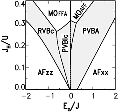
Figure 31: The same as in Fig. 12, but including quantum fluctuations as determined in RPA. The spin liquid (RVBc, PVBIc, PVBIa, and PVBA) takes over in the shaded region between G-AF and A-AF phases (after Ref. Fei97 ).

Summarizing, there is a strong theoretical arguments supporting the conjecture that quantum-melting might occur in orbital degenerate MHI. Why does it not occur always (e.g., in KCuF₃)? Next to the Hund’s rule coupling, the electron-phonon coupling $\lambda$ (7) may destroy quantum disorder. The lattice will react to the orbital fluctuations, dressing them up in analogy with polaron physics, and thereby reducing the coupling constant. In order to quantum melt KCuF₃-like states, one should therefore look for ways to reduce both the effective $J_{H}$ and $\lambda$. It was first suggested in Ref. Fei97 that this situation might occur in LiNiO₂: although the spin-spin interactions in the (111) planes should be very weakly FM according to the Goodenough-Kanamori rules, magnetic LRO is absent Hir85 and the system might represent the spin-orbital liquid. More strikingly, LiNiO₂ is cubic and should undergo a collective JT transition, which absence is actually an old chemistry mystery! Upon electron-hole transformation, $d^{7}$ low-spin Ni³⁺ maps on $d^{9}$ Cu²⁺ in KCuF₃, but with a difference in chemistry. While the $e_{g}$ hole in KCuF₃ is nearly entirely localized on the Cu, the $e_{g}$ electron in LiNiO₂ is rather strongly delocalized over the Ni and surrounding O ions which reduces both $J_{H}$ and $\lambda$, and explains the absence of classical ordering. A more precise experimental characterization of LiNiO₂ is needed to decide whether it provides an example for a quantum disorder of the kind discussed here.

Comparing with spin models, the understanding of the disordered ground states in spin-orbital models is much less developed. We have discussed in this Section only these results which could be obtained so far using simple methods based on variational wave functions of the VB and RVB type. There are a few questions which deserve a future study. For instance, by deriving similar rules to those known for the spin systems Sut88 , for calculating the overlaps between different VB-type configurations on the lattice would simplify the analysis of these situations in which the resonance of different configurations might play a role in spin-orbital systems. Formulating the problem on the abstract level, one might attempt to find parent Hamiltonians similar to the AKLT models (150) to particular dimerized states with alternating spin and orbital singlets. However, the $e_{g}$ orbitals are more classical than the pseudospins in the symmetric SU(4) model of Sec. IV.A. Further studies should clarify to what extent the $e_{g}$ orbitals exhibit really quantum behavior in realistic situations, such as described by the $d^{9}$ model (57)–(59). However, we believe that even if the orbitals are more classical than the spins, they amplify the quantum effects just by their fluctuations which couple to spin fluctuations.

V Spin-orbital model in manganites

V.1 Superexchange and orbital interactions in LaMnO₃

As we have shown in Fig. 4, the phase diagrams of manganites are very rich and one would like to understand the microscopic origin of the experimentally observed A-AF order in LaMnO₃ Wol55 in first place, and next why the magnetic interactions change so drastically that the system becomes FM at larger doping. Naively, the FM order follows just from the DE model as presented in Sec. II.B. However, we have presented arguments in Sec. I that this qualitative argument does not explain the physics of manganites and the realistic approach has to include the double degeneracy of $e_{g}$ orbitals occupied by one or less electron per Mn ion.

As we already know from the earlier studies Kug82 ; Goo55 and from Sec. III of the present paper, the magnetic order is coupled to the orbital one. Therefore, one possible explanation of the observed A-AF phase might be that it follows from a cooperative JT effect Mil96 which stabilizes a particular order of the singly occupied $e_{g}$ orbitals Kug73 . Although this might sound quite attractive and attempts were made to understand the superexchange constants observed in the A-AF phase of LaMnO₃ in ab initio calculations Sol96 ; Mry97 , these studies did not give the superexchange constants close to their experimental values. A model of degenerate $e_{g}$ orbitals Marco is more successful, but only when the orbital ordering is not calculated but fitted to the experiment. Here we argue that the leading mechanism comes instead from strong Coulomb interaction $U$ is the dominating energy scale in late transition metal oxides which gives superexchange induced by the hopping of $e_{g}$ electrons Fei99 . At the same time the coupling to the lattice is much smaller than the Coulomb interactions which is consistent with the existence of the insulating phase above the JT transition Pat99 . Of course, the JT effect has to be included in a complete model, as we will also show below, as it leads to particular orbital interactions and stabilizes the orbital ordering well before (when the temperature is decreased) the magnetism sets in. Therefore, we believe that the JT effect is of crucial importance in the doped regime where it drives the transition from the insulating polaronic regime to a metal MMS96 .

If transition metal ions have partly filled $e_{g}$ orbitals close to orbital degeneracy, as we have discussed for the KCuF₃, the strong Coulomb interactions lead to an effective low energy Hamiltonian, where the spin and orbital degrees of freedom are coupled Kug73 ; Fei97 ; Ole00 . As an important difference with respect to the d⁹ configuration (Sec. III.A), one has to construct superexchange between total spins $S=2$ of Mn³⁺ ions in LaMnO₃ compound Fei99 . A simpler approach in which the superexchange is considered separately for the $e_{g}$ electrons with spins $s=1/2$ and for $t_{2g}$ electrons with spins $S_{t}=3/2$ Ish97 ; Ish00 is not realistic as the spin dynamics of $e_{g}$ and $t_{2g}$ spins does not occur independently of each other and the spin waves measured by neutrons correspond to the spin excitations of spins $S=2$ Hir96 ; Hir96a . This simplified approach proposed recently by Ishihara, Inoue and Maekawa Ish97 emphasizes correctly the role of orbitals, but violates the SU(2) spin symmetry and involves a Kondo coupling $K$ between $e_{g}$ and $t_{2g}$ spins, which by itself is not a faithful approximation to the multiplet structure, as we explain below. The complete effective model of the undoped LaMnO₃ has to include also the $t_{2g}$-part of superexchange and the orbital interactions induced by the JT effect Fei99 . We will show that these terms, while unessential qualitatively, are very important for a quantitative understanding.

The superexchange between the $d^{4}$ Mn³⁺ ions originates in the large-$U$ regime from virtual ($e_{g}$ or $t_{2g}$) excitations, $d_{i}^{4}d_{j}^{4}\rightleftharpoons d_{i}^{3}d_{j}^{5}$. The spin-orbital model presented below follows from the full multiplet structure of the manganese ions in octahedral symmetry, both in the $d^{4}$ ($t_{2g}^{3}e_{g}$) configuration of the Mn³⁺ ground state, and in the $d^{3}$ ($t_{2g}^{3}$) and $d^{5}$ ($t_{2g}^{3}e_{g}^{2}$) virtually excited states of Mn⁴⁺ and Mn²⁺ ions, respectively. Our starting point is that each Mn³⁺ ($d^{4}$) ion is in the high-spin ($t_{2g}^{3}e_{g}$) ground state in agreement with large Hund’s rule interaction $J_{H}$, i.e., the high-spin ($S=2$) orbital doublet ${}^{5}\!E$.

Figure 32: Virtual $d_{i}^{4}d_{j}^{4}\rightarrow d_{i}^{3}d_{j}^{5}$ excitations which generate effective interactions for a bond $(ij)\parallel c$-axis: (a) for one $|x\rangle$ and one $|z\rangle$ electron, and (b) for two $|z\rangle$ electrons (after Ref. Fei99 ).

First, we analyze the strongest channel of superexchange, which follows from the hopping of $e_{g}$ electrons between nearest neighbor sites $i$ and $j$. The derivation is similar to that analyzed in detail for the $d^{9}$ configuration in Sec. III.A, but the important difference is found in the spin sector, where the derived effective interactions have to be represented by the superexchange terms between total spins $S=2$ per site Fei99 . When we consider a bond oriented along the cubic $c$-axis, only a $3z^{2}-r^{2}$ electron can hop as in the $d^{9}$ case (Sec. III.A), and four $d^{5}$ states may be reached: the high-spin ${}^{6}\!A_{1}$ state ($S=5/2$), and the lower-spin ($S=3/2$) ${}^{4}\!A_{1}$, ${}^{4}\!E$, and ${}^{4}\!A_{2}$ states (Fig. 32). The $d_{i}^{4}d_{j}^{4}\rightleftharpoons d_{i}^{3}(t_{2g}^{3})d_{j}^{5}(t_{2g}^{3}e_{g}^{2})$ excitation energies require for their description in principle all three Racah parameters, $A$, $B$ and $C$ Gri71 : $\varepsilon(^{6}\!A_{1})=A-8B$, $\varepsilon(^{4}\!A_{1})=A+2B+5C$, $\varepsilon(^{4}\!E)\simeq A+6B+5C$, $\varepsilon(^{4}\!A_{2})=A+14B+7C$. In view of the realistic values of $B=0.107$ and $C=0.477$ eV for Mn²⁺ ($d^{5}$) ions Boc92 , one may use an approximate relation $C\simeq 4B$, and write the excitation energies in terms of Coulomb, $U\equiv A+2B+5C$, and Hund’s exchange, $J_{H}\equiv 2B+C\simeq 0.69$ eV, parameters:

$$\varepsilon(^{6}\!A_{1}) = U-5J_{H},$$ (153)

$$\varepsilon(^{4}\!A_{1}) = U,$$ (154)

$$\varepsilon(^{4}\!E\,) = U+\frac{2}{3}J_{H},$$ (155)

$$\varepsilon(^{4}\!A_{2}) = U+\frac{10}{3}J_{H}.$$ (156)

We emphasize that $U$ is here by definition not the Coulomb matrix element, but the reference energy of the $|^{4}\!A_{1}\rangle$ state; this definition is different from some other conventions Boc92 ; Miz95 . A value of $U=7.3$ eV was deduced for LaMnO₃ by Feiner and Oleś Fei99 from the available spectroscopic data Zaa90 ; Boc92 ; Miz95 .

Using the spin algebra (Clebsch-Gordon coefficients), the reduction of product representations in cubic site symmetry Gri71 for the intermediate states, and making a rotation of the terms derived for a bond $\langle ij\rangle\parallel c$ to the bonds $\rangle ij\langle\parallel a$ and $\rangle ij\langle\parallel b$ as in Sec. III.A, one finds a compact expression,

$$H_{J}(e_{g}) = \frac{1}{16}\sum_{\langle ij\rangle}\left\{-\frac{8}{5}\frac{t^{2}}{\varepsilon(^{6}\!A_{1})}\left(\vec{S}_{i}\cdot\vec{S}_{j}+6\right){\cal P}_{\langle ij\rangle}^{\zeta\xi}\right.$$ (157)

$$\hskip 28.45274pt\left.+\left[\frac{t^{2}}{\varepsilon(^{4}\!E)}+\frac{3}{5}\frac{t^{2}}{\varepsilon(^{4}\!A_{1})}\right]\left(\vec{S}_{i}\cdot\vec{S}_{j}-4\right){\cal P}_{\langle ij\rangle}^{\zeta\xi}\right.$$

$$\hskip 28.45274pt\left.+\left[\frac{t^{2}}{\varepsilon(^{4}\!E)}+\frac{t^{2}}{\varepsilon(^{4}\!A_{2})}\right]\left(\vec{S}_{i}\cdot\vec{S}_{j}-4\right){\cal P}_{\langle ij\rangle}^{\zeta\zeta}\right\},$$

where $t$ is the hopping element along the $c$-axis, while ${\cal P}_{\langle ij\rangle}^{\zeta\xi}$ and ${\cal P}_{\langle ij\rangle}^{\zeta\zeta}$ are the projection operators introduced in Eqs. (60) and (61). A similar expression was derived by Shiina, Nishitani and Shiba using the group theory arguments Shi97 . However, this method does not allow to determine accurately the coefficients of different terms, and thus the balance between AF and FM interactions is different.

The terms in the first line of Eq. (157) are obtained from the virtual processes which involve different occupancies at the sites $i$ and $j$ – at one site the orbital along the bond $|\zeta\rangle$ is occupied by an $e_{g}$ electron, while an orthogonal orbital $|\xi\rangle$ is occupied at the other [Fig. 32(a)]. In agreement with the general rule as presented in Secs. I and III.A, the processes which involve the high-spin state $|^{6}\!A_{1}\rangle$ lead to FM superexchange, while the low-spin state $|^{4}\!A_{1}\rangle$ gives an AF interaction. The terms in the second line arise from the configurations with occupied directional orbitals $|\zeta\rangle$ at both sites which give the excited states with a double occupancy in one of the $|\zeta\rangle$ orbitals [Fig. 32(b)]. After projecting this double occupancy onto the eigenstates $|^{4}\!E\rangle$ and $|^{4}\!A_{2}\rangle$ one finds the AF interactions. Thus, the structure is similar to that of Eq. (58), but the coefficients are different and follow from the multiplet structure of the excited $d^{5}$ states and from the spin algebra.

A similar derivation gives the $t_{2g}$ superexchange Fei99 ,

$$H_{J}(t_{2g})=\frac{1}{4}J_{t}\sum_{\langle ij\rangle}\left(\vec{S}_{i}\cdot\vec{S}_{j}-4\right),$$ (158)

where $J_{t}$ is an average of the processes which couple different low-spin $d^{5}$ ($t_{2g}^{4}e_{g}$) and $d^{3}$ ($t_{2g}^{3}$) excited states ${}^{4}T_{1}$ and ${}^{4}T_{2}$ of Mn²⁺ and Mn⁴⁺ ions, respectively, $J_{t}=(J_{11}+J_{22}+J_{12}+J_{21})/4$. The individual exchange elements, $J_{mn}=t_{\pi}^{2}/\varepsilon(^{4}T_{m},^{4}\!T_{n})$, result from different local $d_{i}^{4}d_{j}^{4}\rightleftharpoons d_{i}^{5}(t_{2g}^{4}e_{g})d_{j}^{3}(t_{2g}^{2}e_{g})$ excitations within an $\langle ij\rangle$ bond, with energies $\varepsilon(^{4}T_{1},^{4}\!T_{1})\simeq U+8J_{H}/3$, $\varepsilon(^{4}T_{1},^{4}\!T_{2})\simeq U+2J_{H}/3$, $\varepsilon(^{4}T_{2},^{4}\!T_{1})\simeq U+4J_{H}$, $\varepsilon(^{4}T_{2},^{4}\!T_{2})\simeq U+2J_{H}$, expressed by the same elements $U$ and $J_{H}$ as above, where the states ${}^{4}T_{m}$ (${}^{4}T_{n}$) label the symmetry of $d_{i}^{5}$ ($d_{j}^{3}$) excited configurations, respectively. The hopping element between the $t_{2g}$ orbitals involves two-step processes via the oxygen orbitals in bridge positions (see Fig. 1), and thus one finds that $t_{\pi}=t/3$. We neglected the correction terms which describe the anisotropy of $t_{2g}$ superexchange depending on the actual configuration of $e_{g}$ electrons.

As we already pointed out, the complete spin-orbital model for the undoped manganites Fei99 ,

$${\cal H}=H_{J}(e_{g})+H_{J}(t_{2g})+H_{\rm JT}+H_{\tau},$$ (159)

includes both above superexchange terms due to $e_{g}$ and $t_{2g}$ excitations [$H_{J}(e_{g})$ and $H_{J}(t_{2g})$], the effective interactions between orbital degrees of freedom which follow from the JT effect ($H_{\rm JT}$), and a low-symmetry crystal field ($H_{\tau}$). The JT term may be derived from the general energy expression (15) for the cooperative JT effect Mil96 . The operator form of the intersite orbital interaction $\propto\kappa$ (15),

$$H_{\rm JT}=\kappa\sum_{\langle ij\rangle}\left({\cal P}_{\langle ij\rangle}^{\zeta\zeta}-2{\cal P}_{\langle ij\rangle}^{\zeta\xi}+{\cal P}_{\langle ij\rangle}^{\xi\xi}\right)=2\kappa\sum_{\langle ij\rangle}\left(1-2{\cal P}_{\langle ij\rangle}^{\zeta\xi}\right),$$ (160)

favors orbital alternation, i.e., one $|\zeta\rangle$ and one $|\xi\rangle$ as occupied orbitals at two ends of the same bond $\langle ij\rangle$. In analogy to Eqs. (60) and (61) we define ${\cal P}_{\langle ij\rangle}^{\xi\xi}=2P_{i}^{\xi}P_{j}^{\xi}$. The second equality in Eq. (160) follows from the completeness relation, ${\cal P}_{\langle ij\rangle}^{\zeta\zeta}+2{\cal P}_{\langle ij\rangle}^{\zeta\xi}+{\cal P}_{\langle ij\rangle}^{\xi\xi}=2$. The coefficient $\kappa$ is a parameter which was estimated in Ref. Fei99 from the experimental temperature of the structural phase transition $T_{s}$. Eq. (160) gives therefore the same energetically favored orbital configurations as those involved in the superexchange terms in Eq. (157) which occur due to the $|^{6}\!A_{1}\rangle$ and $|^{4}\!A_{1}\rangle$ excited states. The last term is the crystal-field splitting of the $e_{g}$ orbitals (59) which we reproduce here for completeness,

$$H_{\tau}=-E_{z}\sum_{i}\tau_{i}^{c}.$$ (161)

The strength of $e_{g}$ and $t_{g}$ superexchange can be estimated fairly accurately from the basic electronic parameters for the Mn ion as determined from spectroscopy Zaa90 ; Boc92 ; Miz95 , with an estimated accuracy of $\sim 20\%$. Using $U=7.3$ eV and $J_{H}=0.69$ eV, and taking into account that the Mn-Mn hopping occurs in effective processes via the bridging oxygen, one finds $t=0.41$ eV which follows from $t=t_{pd}^{2}/\Delta$, with Mn-O hopping $t_{pd}=1.5$ eV and charge transfer energy $\Delta=5.5$ eV. This yields $J=t^{2}/U=23$ meV which we take as a measure of the $e_{g}$-part of superexchange, and $J_{t}=2.1$ meV. The accuracy of these parameters may be appreciated from the resulting prediction for the Néel temperature of CaMnO₃, where a similar derivation gives for spin $S=3/2$,

$$\hat{H}_{t}=\hat{J}_{t}\sum_{\langle ij\rangle}\left(\frac{4}{9}\vec{S}_{i}\cdot\vec{S}_{j}-1\right),$$ (162)

where $\hat{J}_{t}\simeq J_{t}(1+J_{H}/U)$. Using the estimates from spectroscopy, one obtains $\hat{J}_{t}=4.6$ meV and thus $T_{N}=124$ K Fei99 , in excellent agreement with the experimental value $T_{N}=110$ K Wol55 .

Here it is worthwhile to discuss the difference between the present approach and the popular simplified model introduced by Ishihara, Inoue, and Maekawa Ish97 . These authors also emphasized the role of orbital variables in the $e_{g}$-superexchange, but assumed that the total spin is conserved within the $e_{g}$-subband, and one can thus use the same derivation as presented in Sec. III.A, with the excitation energies adopted to the new situation when the $e_{g}$ electrons interact also with the $t_{2g}$ core states by the Hund’s rule interaction $K$ between one $e_{g}$ and one $t_{2g}$ electron defined in the same way as in Eq. (23). Although the original notation was somewhat more involved Ish97 , using our projection operators (60) and (61), and the spin projection operators (21), their result may be rewritten as follows,

$${H}_{\rm IIM} = \sum_{\langle ij\rangle}\left\{-\frac{t^{2}}{\bar{U}^{\prime}-\bar{J}_{H}}\left(\vec{S}_{i}\cdot\vec{S}_{j}+\frac{3}{4}\right){\cal P}_{\langle ij\rangle}^{\zeta\xi}+\frac{t^{2}}{\bar{U}^{\prime}+\bar{J}_{H}+K}\left(\vec{S}_{i}\cdot\vec{S}_{j}-\frac{1}{4}\right){\cal P}_{\langle ij\rangle}^{\zeta\xi}\right.$$ (163)

$$\hskip 22.76228pt\left.+\frac{2t^{2}}{\bar{U}+K}\left(\vec{S}_{i}\cdot\vec{S}_{j}-\frac{1}{4}\right){\cal P}_{\langle ij\rangle}^{\zeta\zeta}\right\},$$

Therefore, the multiplet structure given by Eqs. (153)–(156) is now replaced by:

$$\varepsilon(^{6}\!A_{1}) \simeq \bar{U}^{\prime}-\bar{J}_{H},$$ (164)

$$\varepsilon(^{4}\!E\,) \simeq \bar{U}^{\prime}+\bar{J}_{H}+K,$$ (165)

$$\varepsilon(^{4}\!A_{2}) \simeq \bar{U}+K.$$ (166)

It is evident that the Hamiltonian (163) is not equivalent to the expression derived using the correct multiplet structure as given by Eq. (157) Fei99 . First of all, note that $\bar{J}_{H}$ has here the same meaning as the Hund’s rule element used to describe the exchange interactions between a pair of $d$ electrons. Then the excitation spectrum (164)–(166) should be equivalent to the excitation spectrum given by Eqs. (42)–(45) in the absence of $t_{2g}$ spins at $K=0$. The correspondence between the Coulomb and exchange elements in Eqs. (163) and (1) is given by $\bar{U}^{\prime}=U-J_{H}$ and $\bar{J}_{H}=J_{H}$, and the first two energies of the $|e_{g}^{2}\rangle$ excited state agree, but the highest energy does not. The reason is that the intraorbital Coulomb interaction $\bar{U}$ is not an independent parameter, but $\bar{U}=\bar{U}^{\prime}+2\bar{J}_{H}$ Ole83 . Second, the state $|^{4}\!A_{2}\rangle$ comes out to be doubly degenerate in Eq. (163) as the processes $\propto\bar{J}_{H}$ which transfer a pair of electrons with opposite spins between different orbitals in Eq. (1) were not included and thus the doublet occurs as the highest-energy state rather than the state in the middle. Furthermore, for the choice of parameters of Ref. Ish97 with $\bar{U}^{\prime}=5$, $\bar{U}=7$ and $\bar{J}_{H}=2$ eV, not only the structure of levels is incorrect, but even the $|^{4}\!E\rangle$ and $|^{4}\!A_{2}\rangle$ states have accidental degeneracy. Third, the parameter $K$ in the case of $d_{i}^{4}d_{j}^{4}\rightleftharpoons d_{i}^{3}(t_{2g}^{3})d_{j}^{5}(t_{2g}^{3}e_{g}^{2})$ excitations is not a free parameter, but $K=3\bar{J}_{H}$ (the factor of three comes about due to three $t_{2g}$ electrons which form a large spin $S=3/2$ interacting with an $e_{g}$ electron by the Kondo term). This last condition is obeyed by the actual choice of parameters in Ref. Ish97 . Finally, the state $|^{4}\!A_{1}\rangle$ has been completely missed in Eqs. (164)–(166). Therefore, we conclude that the Hamiltonian (163): (i) violates the SU(2) invariance of superexchange interactions in spin space, and (ii) does not correspond to the correct multiplet structure of $d^{5}$ ions in any nontrivial limit. A common feature with Eq. (157) is that FM interactions are enhanced due to the lowest excited $|^{6}\!A_{1}\rangle$ state, but the dependence of the magnetic interactions on ${\bar{J}}_{H}$ is quite different, and it gives a different answer concerning the stability of the A-AF phase.

The model of Ishihara et al. Ish97 contains also a superexchange term between core spins $t_{2g}$ which takes the same form as that given in Eq. (162). In contrast to the present derivation of Ref. Fei99 , no formula for the interaction $\hat{J}_{t}$ was derived in Ref. Ish97 , but instead the value of $\hat{J}_{t}$ was fitted in order to reproduce the stable A-AF ordering, as observed in LaMnO₃. This results in a value of $\hat{J}_{t}$ overestimated by a factor close to seven and having no relation to the experimental value of the Néel temperature for CaMnO₃.

A comparison between Eqs. (157) and (163) is possible only when the magnetic interactions concern the same spins $S=2$. Therefore, we have renormalized the terms $\sim t^{2}/\varepsilon_{n}$, where $\varepsilon_{n}$ is the excitation energy, and $\hat{J}_{t}$ in the model of Ishihara, Inoue and Maekawa Ish97 to act on the total spins $S=2$. After this modification, the superexchange terms obtained from both models may be written in the same form:

$${\cal H}_{SE}=\sum_{\langle ij\rangle}\left(-J_{1}{\cal P}_{\langle ij\rangle}^{\zeta\xi}+J_{2}{\cal P}_{\langle ij\rangle}^{\zeta\xi}+J_{3}{\cal P}_{\langle ij\rangle}^{\zeta\zeta}+J_{AF}\right)\vec{S}_{i}\cdot\vec{S}_{j},$$ (167)

where the first interaction $\propto J_{1}$ is FM, and the remaining interactions are AF. We present the values of different constants in Table 2. First of all, the superexchange terms are much smaller than the hopping integral $t$ which justifies a posteriori the perturbative approach. Second, taking the multiplet structure of Mn²⁺ ions one finds a competition between the FM and AF contributions to the $e_{g}$-promoted superexchange (157), with the AF terms being roughly half of the largest FM term Fei99 . As we show below, this ratio between the FM and AF interactions gives automatically the A-AF order as observed in LaMnO₃.

In contrast, the (effective) interactions $J_{n}$ found from Eq. (163) are not balanced due to overestimated excitation energies $\varepsilon_{n}\simeq 13.0$ eV to the low-spin states ($n=2,3$). On one hand, one finds a dominating FM term $J_{1}=3.48$ meV, not far from $J_{1}=4.40$ meV found from Eq. (157), while on the other hand the AF terms are smaller by a factor close to two. Therefore, the $e_{g}$ part of the superexchange alone gives a FM state in all three directions, and one is forced to simulate the missing AF interactions by a large superexchange term coming from the hopping of $t_{2g}$ electrons Ish97 (see Table 2). Another consequence of too low values of $J_{2}$ and $J_{3}$ is a rather narrow parameter regime for the stable A-AF order, much narrower than in the approach using the correct multiplets, where the A-AF order is generic Fei99 .

Table 2: Magnetic interactions $J_{n}$ in Eq. (167), and the excitation energies $\varepsilon_{n}$ used in perturbation theory, as obtained from the $d^{4}$ spin-orbital model (157) Fei99 and from the model of Ishihara, Inoue and Maekawa (163) Ish97 . The excitation energies $\varepsilon_{2}$ and $\varepsilon_{3}$ in the case of Eq. (157) were averaged over two states which contribute to $J_{n}$.

		model (157) Fei99			model (163) Ish97
superexchange	orbital operator	$\varepsilon_{n}$ (eV)	$J_{n}$ (meV)	$J_{i}/t$ ($10^{-2}$)	$\varepsilon_{n}$ (eV)	$J_{n}$ (meV)
$J_{1}$	${\cal P}^{\zeta\xi}_{\langle ij\rangle}$	3.80	4.40	1.07	3.0	3.48
$J_{2}$	${\cal P}^{\zeta\xi}_{\langle ij\rangle}$	7.53	2.21	0.54	13.0	0.81
$J_{3}$	${\cal P}^{\zeta\zeta}_{\langle ij\rangle}$	8.68	2.44	0.60	13.0	1.62
$J_{AF}$	–	8.91	0.53	0.13	–	3.50

The classical phases found in the present $d^{4}$ model (Fig. 33) are similar to those shown before in Fig. 11, but at present the spins of $e_{g}$ and $t_{2g}$ electrons are aligned and form total spins $S=2$. Due to the identical interactions in the orbital sector, the MF phase diagram of the $e_{g}$-part of the manganese $d^{4}$ model (159), $H=H_{J}(e_{g})+H_{\tau}$, at $T=0$ is similar to that of the cuprate $d^{9}$ spin-orbital model (57) Fei97 ; Ole00 analyzed in Sec. III.B: at large positive (negative) $E_{z}$, one finds AF phases with either $|x\rangle$ (AFxx) or $|z\rangle$ (AFzz) orbitals occupied, while MO phases with occupied orbitals given as linear combinations (65) of the basis states $|x\rangle$ and $|z\rangle$ are favored by increasing $J_{H}$. As in the $d^{9}$ case, the $e_{g}$ part of superexchange (157) is frustrated at $J_{H}=0$ and $E_{z}=0$. However, due to the large value of total spin $S=2$, the quantum corrections are expected to be much smaller and we may assume that the classical order is robust, at least certainly at finite $J_{H}$ and in the presence of $t_{2g}$ AF superexchange (158).

Figure 33: Classical phase diagram of the manganite model (159): (a) no JT effect ($\kappa=0$): $J_{t}=0$ (full lines) and $J_{t}=0.092J$ (dashed lines), with the AFxx and AFzz phases separated by a MOAAA phase; (b) including JT effect ($\kappa=0.5J$): $J_{t}=0$ (dashed lines) and $J_{t}=0.092J$ (full lines) (after Ref. Fei99 ).

The A-AF order is found at finite $J_{H}/U\simeq 0.1$ [Fig. 33(a)]. If $E_{z}<0$ the spin order is FM (AF) in the $(a,b)$ planes (along the $c$-axis) in the MOFFA phase, while at $E_{z}>0$ two similar phases, MOAFF and MOFAF, are degenerate. For the parameters appropriate for LaMnO₃, with $J_{H}/U\simeq 0.095$, one finds a MOFFA/MOAFF ground state, i.e., A-AF magnetic order, while a FM (MOFFF) phase is stable only at $J_{H}/U>0.12$. The result is therefore qualitatively similar to the classical phase diagram of the $d^{9}$ model (Fig. 12). We emphasize again that the region of stability of the A-AF phase is somewhat modified by $t_{2g}$-superexchange [Fig. 33(a)], but this change is small as $J_{t}\ll J$.

The value of $\kappa$ in Eq. (160) is the only parameter of the manganite model (159) which had to be determined from experiment Fei99 . First of all, the $e_{g}$ part of superexchange alone favors the alternation of orbitals, i.e., maximizes the average $\langle{\cal P}_{\langle ij\rangle}^{\zeta\xi}\rangle$ and one can verify that a structural transition follows already from this term. However, the transition temperature obtained in this way amounts to $T_{s}^{e}\simeq 440$ K (see Fig. 34) and is far below the experimental value of $T_{s}^{exp}\simeq 750$ K. Therefore, the structural phase transition is induced to a larger extent by the orbital interactions generated by the JT effect included via the H_JT term (160). Their contribution to the mean-field value of the transition temperature is equal $T_{s}^{\kappa}=6\kappa$. Using the typical ratio between the MF value $T_{s}$ and the experimental transition temperature $T_{s}^{exp}$ for pseudospins 1/2, $T_{s}/T_{s}^{exp}=1.6$, it follows from $T_{s}=T_{s}^{e}+T_{s}^{\kappa}=1200$ K that $6\kappa\simeq 760$ K. Thus $\kappa\simeq 11$ meV which agrees with the estimate of Millis that $\kappa>10$ meV (where he did not separate the orbital interactions into those originating from the JT effect and from superexchange). Therefore, the representative value $\kappa/J=0.5$ was considered in Ref. Fei99 .

Figure 34: Magnetic transition temperatures $T_{c}$ ($J=23$ meV, $E_{z}=0$, $J_{t}=0.092J$, $\kappa=0.5J$) for: MOAAA (dashed line), MOFFF (long-dashed line), and MOFFA (full line) phases, and $T_{s}$ for the structural (MO) phase transition at $\kappa=0$ (squares). The dotted line indicates realistic $J_{H}/U=0.095$ for LaMnO₃ (after Ref. Fei99 ).

Due to the structural transition which occurs in LaMnO₃ at $T_{s}\simeq 750$ K, one has to use a MF theory for the phases with coupled order parameters, assuming that the order parameters corresponding to $\langle{\vec{S}}\rangle$, $\langle{\vec{\tau}}\rangle$, and $\langle{\vec{S}}{\vec{\tau}}\rangle$ are independent variables Dit80 . When the orbital interactions induced by the JT effect are included via H_JT term (160), one gets with decreasing temperature first a transition due to the largest orbital interactions to the phase with $\langle{\vec{\tau}}\rangle\neq 0$. This induces significant changes in the phase diagram close to the origin $(E_{z},J_{H})=(0,0)$ [Fig. 33(b)]. In fact, the JT coupling $\kappa$ enforces alternating orbitals with $\theta=\pi/4$ in Eqs. (III.2) which stabilizes G-AF spin order in the MOAAA phase at small $J_{H}/U$, while the pure AFxx and AFzz phases are suppressed. However, in the physically interesting regime of larger $J_{H}/U$ the orbital order is mainly driven by the $e_{g}$-superexchange interactions (157). Besides, from Fig. 33 one can see that the A-AF phase is not affected by the JT coupling in the physical regime of parameters for the LaMnO₃.

At finite temperature one may study the competition of different magnetic phases. One finds that the same magnetic phases develop in the presence of orbital ordering at finite temperature (Fig. 34) as those found independently at $T=0$. For the experimental value of $J_{H}/U\simeq 0.095$ the magnetic transition into the A-AF phase is obtained at $T_{N}^{\rm MF}\simeq 148$ K which after reduction gives a prediction for the experimental transition temperature of $T_{N}\simeq 106$ K, in reasonable agreement with the actually observed value of 136 K Kaw96 .

Figure 35: Exchange interactions $J_{(a,b)}$ and $J_{c}$ in the ground state for increasing $J_{H}/U$, for $J=23$ meV and: $J_{t}=0$, $\kappa=0$ (dashed lines), $J_{t}=0.092J$, $\kappa=0$ (long-dashed lines), and $J_{t}=0.092J$, $\kappa=0.5J$ (full lines). The jumps in $J_{(a,b)}$ and $J_{c}$ correspond to phase transitions of Fig. 33. The inset gives the values of $\cos 2\theta$ defined as in Eqs. (III.2), in the same range of $J_{H}/U$ for the optimal orbital state (after Ref. Fei99 ).

As a remarkable success of the model (159), the magnetic interactions obtained for the A-AF phase are close to the experimental values. The FM interactions in the $(a,b)$ planes $J_{(a,b)}$, and the AF interactions along the $c$-axis $J_{c}$ are found from Eqs. (157) and (158) by averaging over the orbital operators in the actual classical ground state (Fig. 35). The values obtained at $J_{H}/U=0.095$: $J_{(a,b)}=-1.15$ meV and $J_{c}=0.88$ meV Fei99 are somewhat larger than the experimental values of -0.83 and 0.58 meV Hir96 ; Hir96a , respectively. It is interesting to realize that although the observed A-AF phase would be obtained from the $e_{g}$ superexchange alone, the ratio of the above exchange constants is then $J_{c}/|J_{(a,b)}|=2.25$. Instead, if the $t_{2g}$ superexchange and the JT term are included in the present model, the value $J_{c}/|J_{(a,b)}|=0.77$ is found which agrees very well with the experimental ratio of 0.7 Hir96 ; Hir96a . The $t_{2g}$ term alone enhances the AF interactions, but does modify the orbital ordering, and gives thus a different ratio $J_{c}/|J_{(a,b)}|=1.04$. Therefore, we conclude that all the interaction terms in Eq. (159) are important in order to explain the experimentally observed exchange interactions in LaMnO₃. These values could not be reproduced up to now by ab initio calculations performed in LSDA which fails even to give the correct sign of $J_{c}$ Sol96 , while the values somewhat closer to experiment and to those of Ref. Fei99 were obtained recently in the HF approximation: $J_{(a,b)}=-0.44$ meV and $J_{c}=0.11$ meV Kap00 .

V.2 Polaronic regime at low hole doping

The spin-orbital model (159) which includes the complete superexchange and the orbital interactions which follow from the JT effect provides a good starting point to describe the interplay between magnetic and orbital interactions in doped manganites. It reproduces very well the spin and orbital pattern observed in the ground state of LaMnO₃ Fei99 which can be well understood as mainly due to the spin and orbital interactions contained in the $e_{g}$ superexchange (157), with small corrections given by the JT effect. Thus, the undoped case involves spin, orbital and lattice degrees of freedom. When the holes are doped into this ordered ground state, the charge degrees of freedom occur in addition and modify the ground state properties. Their understanding represents one of the most challenging and complex problems in the physics of CMR compounds Ima98 ; Ram97 .

We need to generalize the interaction terms which appeared in the undoped case to the present situation, taking into account the constraint which follows from large $U$ that prevents the occupancy of any Mn ion by more that one $e_{g}$ electron. Therefore, we restrict the space to Mn³⁺ and Mn⁴⁺ configurations. Furthermore, at low hole concentrations the doped holes are trapped and form polarons, as follows from the insulating magnetic phases found at low doping in the phase diagrams of Fig. 4. Therefore, a polaronic model was developed in Ref. Sces99 , with the low-energy effective model Hamiltonian given by:

$${\cal H}=H_{J}(e_{g})+H_{J}(t_{2g})+H_{\rm JT}+H_{\tau}+H_{pol}.$$ (168)

It includes superexchange terms due to $e_{g}$ and $t_{2g}$ electrons [$H_{J}(e_{g})$ and $H_{J}(t_{2g})$], orbital interactions ($H_{\rm JT}$), the crystal-field splitting ($H_{\tau}$) induced by the JT effect, and the polaronic energy ($H_{pol}$) which contributes at finite doping with new FM interactions due to the effective processes involving the excitations around a Mn⁴⁺ ion created by a hole.

The superexchange between total spins $S=2$ is generalized with respect to the undoped case by including the constraint on the $e_{g}$ occupation to,

$$H_{J}(e_{g}) = \frac{1}{4}J\sum_{\langle ij\rangle}f_{i}f_{i}^{\dagger}\left\{-\frac{8}{5}\frac{U}{\varepsilon(^{6}\!A_{1})}\left(\frac{1}{4}\vec{S}_{i}\cdot\vec{S}_{j}+\frac{3}{2}\right){\cal P}_{\langle ij\rangle}^{\zeta\xi}\right.$$ (169)

$$\left.\hskip 28.45274pt+\left[\frac{U}{\varepsilon(^{4}\!E)}+\frac{3}{5}\frac{U}{\varepsilon(^{4}\!A_{1})}\right]\left(\frac{1}{4}\vec{S}_{i}\cdot\vec{S}_{j}-1\right){\cal P}_{\langle ij\rangle}^{\zeta\xi}\right.$$

$$\left.\hskip 28.45274pt+\left[\frac{U}{\varepsilon(^{4}\!E)}+\frac{U}{\varepsilon(^{4}\!A_{2})}\right]\left(\frac{1}{4}\vec{S}_{i}\cdot\vec{S}_{j}-1\right){\cal P}_{\langle ij\rangle}^{\zeta\zeta}\right\}f_{j}f_{j}^{\dagger},$$

where $J=t^{2}/U$, and $t$ is the hopping between $3z^{2}-r^{2}$ orbitals along the $c$-axis. The excitation energies are given by Eqs. (153)–(156), and the orbital projection operators have been introduced in Sec. III. The hole operators $f_{i}^{\dagger}$ and $f_{i}$ guarantee that this superexchange term contributes only if both sites carry a single $e_{g}$ electron ($f_{i}f_{i}^{\dagger}=1$), and the orbital operators ${\cal P}_{\langle ij\rangle}^{\zeta\xi}$ and ${\cal P}_{\langle ij\rangle}^{\zeta\zeta}$ decide about the strength of a particular superexchange contribution.

The $t_{2g}$-superexchange is isotropic in leading order,

$$H_{J}(t_{2g}) = \sum_{\langle ij\rangle}\left\{J_{t}\left(\frac{1}{4}\vec{S}_{i}\cdot\vec{S}_{j}-1\right)f_{i}f_{i}^{\dagger}f_{j}f_{j}^{\dagger}+{\hat{J}}_{t}\left(\frac{4}{9}\vec{S}_{i}\cdot\vec{S}_{j}-1\right)f_{i}^{\dagger}f_{i}f_{j}^{\dagger}f_{j}\right.$$ (170)

$$\left.\hskip 14.22636pt+{\bar{J}}_{t}\left(\frac{1}{3}\vec{S}_{i}\cdot\vec{S}_{j}-1\right)\left(f_{i}^{\dagger}f_{i}f_{j}f_{j}^{\dagger}+f_{i}f_{i}^{\dagger}f_{j}^{\dagger}f_{j}\right)\right\},$$

with the AF superexchange constants $J_{t}$, ${\hat{J}}_{t}$, and ${\bar{J}}_{t}$ obtained from the hopping of $t_{2g}$ electrons for the pairs of Mn³⁺–Mn³⁺, Mn⁴⁺–Mn⁴⁺, and Mn³⁺–Mn⁴⁺ ions, respectively. The spin operators $\vec{S}_{i}$ correspond to spins $S=2$ and $S=3/2$ of Mn³⁺ and Mn⁴⁺ ions, when the number of holes at site $i$ is either $f_{i}^{\dagger}f_{i}=0$ or $f_{i}^{\dagger}f_{i}=1$, respectively. The JT term (160) leads to static distortions Mil96 which induce intersite orbital interactions ($\propto\kappa$) between the $e_{g}$ orbitals and is rewritten in a similar way,

$$H_{\rm JT}=\kappa\sum_{\langle ij\rangle}f_{i}f_{i}^{\dagger}\left({\cal P}_{\langle ij\rangle}^{\zeta\zeta}-2{\cal P}_{\langle ij\rangle}^{\zeta\xi}+{\cal P}_{\langle ij\rangle}^{\xi\xi}\right)f_{j}f_{j}^{\dagger}.$$ (171)

The problem of a Mott insulator doped by a low number of holes is one of the fascinating problems in the field of strongly correlated electrons. In the $t$-$J$ model the motion of a hole added to an AF background is hindered by the string effect Shr88 , and the free propagation disappears. In manganites the situation is even more complex due to the presence of lattice and orbital degrees of freedom, which are in first place responsible for hole localization at lower doping concentrations. In fact, in an orbitally degenerate Mott-Hubbard system there exists a direct coupling between holes and orbitals due to the polarization of $e_{g}$ orbitals in the neighborhood of a hole Kil99 . This coupling might be strong enough to form a bound state of a hole with the surrounding orbitals, leading to a dressing of hole by orbital excitations vdB00 (Sec. VII.B), and yielding a strong reduction of the bandwidth. Such orbital-hole bound states lead to an exponential suppression of the bandwidth which makes the system unstable towards hole localization. Here we assume that the holes loose most of their kinetic energy due to the lattice distortions of the breathing mode type (Fig. 3), and only the effective processes survive which excite a hole to its nearest neighbors Sces99 .

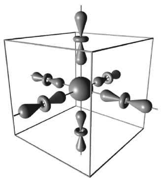
Figure 36: Orbital polaron in the strong coupling limit. Six $|\zeta\rangle$ occupied $e_{g}$ orbitals at Mn³⁺ ions point towards a central hole at a Mn⁴⁺ site (after Ref. Kil99 ).

The cubic symmetry of perovskite manganites is locally broken close to a hole which appears as the removal of the $e_{g}$ degeneracy on the sites adjacent to a doped hole. The origin of this splitting is in the distortions of the oxygen ions that point towards the empty site, and by the electrostatic potential between positive hole and negative electrons. The occupied $e_{g}$ orbitals around a hole are likely to be modified, and if any other orbital interactions were absent, an orbital polaron bound state would be formed around a hole, with occupied $|\zeta\rangle$ orbitals oriented along the bonds towards the hole site (Fig. 36).

In the insulating regime, the localized holes are randomly distributed and form locally lattice polarons with energy $E_{p}$. The new interactions originate from the DE mechanism which induces a FM superexchange for Mn⁴⁺–Mn³⁺ pairs $\propto J_{p}=\bar{J}_{p}/(1+E_{p}/2J_{H})$ (with $\bar{J}_{p}=t^{2}/2E_{p}$) Sces99 ,

$$H_{pol}=-E_{p}\sum_{i}f_{i}^{\dagger}f_{i}-\sum_{\langle ij\rangle}f_{i}^{\dagger}f_{i}\left[\bar{J}_{p}+\frac{1}{8}J_{p}\left(\vec{S}_{i}\cdot\vec{S}_{j}-3\right)\right]P_{j\zeta}f_{j}f_{j}^{\dagger}.$$ (172)

Similar to the undoped case, the exchange terms do depend now on the orientation of the occupied $e_{g}$ orbital on the Mn³⁺ ion by the projection operator $P_{j\zeta}$ (62), with the largest FM contribution when $\langle P_{j\zeta}\rangle=1$, i.e., for the directional $3z^{2}-r^{2}$-type orbitals $|\zeta\rangle$ oriented along the bonds towards the Mn⁴⁺ ion (Fig. 36). The classical phase diagram can be now investigated in a similar fashion as in Sec III.B, assuming that the holes are localized and randomly distributed over the lattice. This assumption corresponds to the dilute limit and describes well the features of polaronic phase in the low doping regime $x=1-n<0.16$.

We have seen that for realistic parameters taken from spectroscopy the A-AF observed in LaMnO₃ at $x=0$ is reproduced (Sec. V.A). Instead of studying the phase diagram as a function of parameters, we address here a simpler question: How the anisotropic exchange constants $J_{(a,b)}=-1.15$ and $J_{c}=0.88$ meV found in LaMnO₃ Fei99 change as a function of doping. Localized polarons in doped systems stabilize locally FM order around Mn⁴⁺ defects as $J_{p}$ is the largest (FM) exchange element, with $J_{p}\simeq 4J$ taking $E_{p}\simeq 0.67$ eV Sces99 , which might provide a natural explanation of a gradual magnetic transition within the insulating phase by the DE mechanism. Indeed, if one assumes that the Mn⁴⁺ are randomly distributed and that the orbital ordering on the Mn³⁺–Mn³⁺ bonds remains unchanged, one finds that the AF coupling $J_{c}$ is gradually weakened with increasing doping $x$, while the FM interaction $|J_{(a,b)}|$ increases much slower (Fig. 37), in good agreement with recent experiments Mou99 . However, a good agreement with the experimental points was obtained assuming that the occupied orbitals around a hole are not modified to $|\zeta\rangle$ orbitals shown in Fig. 36. In contrast, if the directional orbitals $|\zeta\rangle$ are assumed, a much faster transition to the FM phase follows (Fig. 37) which does not agree with experiment. This suggests that the structure of polaron is rather rigid and determined primarily by lattice distortions and local JT effect rather than by the electronic interactions. It might be that some corrections to the perturbative treatment which leads to Eq. (172) are needed, but the present result suggests that the polarons realized in La_1-xSr_xMnO₃ are not orbital polarons of Fig. 36.

Figure 37: Exchange interactions $J_{(a,b)}$ and $J_{c}$ in the A-AF and FMI ground state of La_1-xCa_xMnO₃ ($J_{H}/U=0.095$, $\kappa=0.5J$, $E_{p}=0.67$ eV) for rigid orbital order (full lines) and with $|\zeta\rangle$-type occupied $e_{g}$ orbitals around Mn⁴⁺ ions as in Fig. 36 (dashed lines). The experimental data points Mou99 are shown by filled circles (after Ref. Sces99 ).

A better understanding of polarons is very important in order to get more insight into the observed insulator-metal transition from the insulating to metallic FM phase with increasing doping. It is experimentally observed that La_1-xCa_xMnO₃ is metallic with FM LRO for hole concentrations in the range of $0.17<x<0.5$. This metallic state can be turned into an insulating one by increasing the temperature above the Curie temperature T_C, or by decreasing the hole concentration below x${}_{crit}\simeq 0.17$.

The character of the first transition, from a metallic ferromagnet to an insulating paramagnetic state, can be addressed at first sight in the framework of the interplay between the DE mechanism and the lattice-polaron formation Mil99 . Indeed, in this case the crossover from metallic to insulating state is controlled by the ratio $\lambda=E_{b}/E_{kin}$ of polaron binding energy $E_{b}$ to the average kinetic energy $E_{kin}$ of the charge carriers. The formation of a bound state with the lattice distortion is favored only if the loss in kinetic energy is balanced by a gain in the binding energy. This condition can be reached by raising the temperature in the DE system, since the loss of FM correlations is accompanied by a shrinking of the bandwidth, so that it eventually increases the value of $\lambda$ and induces a carrier localization.

A different situation is represented by the metal-insulator transition induced by the varying hole concentration within the FM phase at low temperature. The total Hamiltonian in the metallic phase has to include explicitly the kinetic energy of $e_{g}$ electrons determined by the symmetry of allowed hopping processes, as presented in Sec. VI. One arrives at the effective $t$-$J$ like model which is characterized by two energy scales for orbital and charge excitations: $W_{orb}$ and $W_{ch}$. Assuming that the orbitals are disordered, i.e., in an orbital liquid state Nag97 , the former quantity describes the orbital fluctuations determined by the value of $J$, and a fraction of the hopping amplitude proportional to the hole density $\propto xt$ which follows from strong correlations (see Sec. VI.B). The quantity $W_{ch}$ determines the rate of the charge fluctuations and the amount of free kinetic energy, determined the bandwidth of $6t$, which corresponds to the uncorrelated electrons.

If the orbitals order, the charge fluctuations are reduced, i.e., the kinetic energy is lowered below its value in a correlated metal. Since the holes can move coherently even within an antiferro-type orbital arrangement vdB00 , it has been argued Kil99 that the reduction of the kinetic energy is only of $\sim 5\%$ including the incoherent processes, while it amounts to $\sim 30\%$ without these contributions. This suggests that orbital ordering cannot suffice to explain the observed localization and one might expect that a more plausible mechanism of localization involves either the formation of orbital polarons, as proposed recently by Kilian and Khaliullin Kil99 , or the lattice deformations.

In summary, the crossover from a free-carrier to a small-polaron picture can be triggered in a DE system either by a reduction of the doping concentration, or by an increase in temperature; the former acts via an enhancement of the polaron binding energy, while the latter by constraining the motion of holes via the DE mechanism. An interesting suggestion that orbital polarons play a major role in both transitions was put forward recently Kil99 . It seems, however, that lattice contribution to localization is more important and the question about the possible role of orbital polarons remains open.

VI Electronic structure and excitations in doped manganites

VI.1 Double exchange in uncorrelated $e_{g}$ orbitals

As we have already shown, the orbital degeneracy gives a rich structure of superexchange which contains competing FM and AF terms, and allows thus for the formation of anisotropic magnetic structures, both in cuprates (Sec. III.A) and in manganites (Sec. V.A). In this Section we will discuss a problem of double-exchange via degenerate orbitals in doped manganites. It is easier to consider first a simpler situation with only few electrons in the $e_{g}$ band that is realistic, for example, for Ca_1-ySm_yMnO₃ Mai98 , where $y\ll 1$ ($y=1-x$ for conventional notation as used in La_1-xA_xMnO₃). For $y=0$ this system is a Mott insulator, with high-spin states $S=3/2$ per site due to the $t_{2g}$ orbitals filled by three electrons, while $e_{g}$ states are empty. Upon doping electrons enter into the doubly degenerate $e_{g}$ orbitals ($E_{z}=0$). In Ca_1-ySm_yMnO₃ a canted spin structure was observed for $0.07<x<0.12$ Mai98 . Other data show that C-AF order is realized in Nd_1-xSr_xMnO₃ for $0.6<x<0.8$, while A-AF phase is stable for $0.5<x<0.6$ Aki98 . In Pr_1-xSr_xMnO₃ the A-AF order exists for $0.5<x<0.7$ Kaw97 .

The effective Hamiltonian which describes the low energy properties of electron doped manganites and represents a generalization of the DE model to degenerate orbitals may be written in the form suggested by van den Brink and Khomskii Bri99 ,

$$H=-\sum_{\langle ij\rangle\alpha\beta\sigma}t_{ij}^{\alpha\beta}(c_{i\alpha\sigma}^{\dagger}c_{j\beta\sigma}+H.c.)-J_{H}\sum_{i\alpha\sigma\sigma{{}^{\prime}}}{\vec{S}}_{i}\cdot c_{i\alpha\sigma}^{\dagger}\vec{\sigma}_{\sigma\sigma{{}^{\prime}}}c_{i\alpha\sigma{{}^{\prime}}}+J_{AF}\sum_{\langle ij\rangle}{\vec{S}}_{i}\cdot{\vec{S}}_{j}.$$ (173)

The first term describes the kinetic energy of $e_{g}$ electrons which are labeled by the site index $i$, spin index $\sigma$, and also by the orbital index $\alpha(\beta)=1,2$, corresponding to the local basis, e.g., to the $|x\rangle$ and $|z\rangle$ orbitals. As in the DE model, $e_{g}$ electrons interact by Hund’s rule exchange $\propto J_{H}$ with core $t_{2g}$ spins, and the model is made more realistic by adding the superexchange between $t_{2g}$ spins $\propto J_{AF}$ which might be determined as in Sec. V.A. However, for the present purpose it was treated as a parameter Bri99 . The presence of the orbital degeneracy, together with the very particular relations between the hopping matrix elements $t_{ij}^{\alpha\beta}$ Sla54 ; Zaa93 , makes this problem and its outcome very different from the usual DE model (Sec. II.B).

The quasiclassical approach to study the model (173) follows the standard route as for the DE mechanism for electrons which move in a nondegenerate band And55 . In the first step we have to determine the spectrum of the $e_{g}$-electrons ignoring their interaction with the localized spins. This spectrum is given by the solution of the matrix equation Tak98 ,

$$||t_{\mu\nu}-\epsilon\delta_{\mu\nu}||=0,$$ (174)

where

$$t_{11} = -2t_{ab}(\cos k_{x}+\cos k_{y}),$$ (175)

$$t_{12} = t_{21}=-\frac{2}{\sqrt{3}}t_{ab}(\cos k_{x}-\cos k_{y}),$$ (176)

$$t_{22} = -\frac{2}{3}t_{ab}(\cos k_{x}+\cos k_{y})-\frac{8}{3}t_{c}\cos k_{z}.$$ (177)

Here $t_{11}$ is the dispersion due to an overlap between two $|x\rangle$ orbitals, $t_{12}$ — between a pair of different orbitals, one $|x\rangle$ and one $|z\rangle$ orbital, and $t_{22}$ between two $|z\rangle$ orbitals on neighboring sites. In writing Eqs. (175)–(177) we have taken into account the ratios of different hopping integrals Sla54 ; Zaa93 , which are determined by the symmetry of the $e_{g}$ wave functions, and introduced the notation $t_{ab}$ and $t_{c}$, to be defined further on. The solutions $\epsilon_{\pm}({\vec{k}})$ of Eq. (174) are:

$$\epsilon_{\pm}({\vec{k}}) = -\frac{4t_{ab}}{3}(\cos k_{x}+\cos k_{y})-\frac{4t_{c}}{3}\cos k_{z}$$ (178)

$$\pm \left\{\left[\frac{2t_{ab}}{3}(\cos k_{x}+\cos k_{y})-\frac{4t_{c}}{3}\cos k_{z}\right]^{2}+\frac{4t_{ab}^{2}}{3}(\cos k_{x}-\cos k_{y})^{2}\right\}^{1/2},$$

These bands were obtained in Refs. Tak98 and Bri99 .

Following van den Brink and Khomskii Bri99 , we now take into account the interaction of the $e_{g}$ electrons with the magnetic background. We assume that the underlying magnetic structure is characterized by two sublattices, with a possible canting, so that the angle between neighboring spins in the $(a,b)$-plane is $\theta_{ab}$ and along the $c$-direction is $\theta_{c}$. This rather general assumption covers all magnetic phases shown in Fig. 5 –AF phases: G-type (two-sublattice structure, $\theta_{ab}=\theta_{c}=\pi$), A-type (FM planes coupled antiferromagnetically, $\theta_{ab}=0$ and $\theta_{c}=\pi$), and C-type structures (FM chains coupled antiferromagnetically, $\theta_{ab}=\pi$ and $\theta_{c}=0$), and the FM phase with $\theta_{ab}=\theta_{c}=0$. As assumed in the nondegenerate DE model And55 , we then have the effective hopping matrix elements determined by the spin background: $t_{ab}=t\cos(\theta_{ab}/2)$ and $t_{c}=t\cos(\theta_{c}/2)$. Note that here $t$ is chosen as the hopping element between two $|x\rangle$ orbitals in $(a,b)$ planes, unlike in the other Sections. We show below that solving this problem in the quasiclassical approximation introduced for the nondegenerate DE model (Sec. II.B), the energy spectrum (178) is renormalized by the magnetic order and, because of the orbital-dependent hopping matrix elements in a degenerate system, this results in an anisotropic magnetic structure.

When we dope the system by adding electrons, these go first into states with minimal energy, in our case into the states close to the $\Gamma$-point at ${\vec{k}}=0$. Let us first assume that all doped charges go into the state with the lowest energy, which is strictly speaking only the case for very small doping ($y\simeq 0$), and neglect for the moment the effects promoted by a finite filling of the bands. At the $\Gamma$-point the energies are $\epsilon_{\pm}(0)=-\frac{4}{3}(2t_{ab}+t_{c})\pm\frac{4}{3}|t_{ab}-t_{c}|$. Using this simplifying assumption which overestimates the kinetic energy, the total energy per site of the system containing $y$ electrons reads:

$$E(\theta_{ab},\theta_{c}) = \frac{J}{2}(\cos\theta_{c}+2\cos\theta_{ab})+y\epsilon_{-}({\vec{k}}=0)$$ (179)

$$= -\frac{3J}{2}+2J\cos^{2}(\theta_{ab}/2)+J\cos^{2}(\theta_{c}/2)$$

$$- \frac{4}{3}yt\left[2\cos(\theta_{ab}/2)+\cos(\theta_{c}/2)+|\cos(\theta_{ab}/2)-\cos(\theta_{c}/2)|\right].$$

Minimizing the energy of the doped state (179) over two angles $\theta_{ab}$ and $\theta_{c}$, one encounters two possible situations Bri99 . If $\cos(\theta_{ab}/2)>\cos(\theta_{c}/2)$, then the magnetic structure is A-type-like; in this case the minimization of the energy with respect to the angles $\theta_{ab}$ and $\theta_{c}$ gives

$$\cos\left({\theta_{ab}\over 2}\right)=\frac{t}{J}y,\hskip 28.45274pt\cos\left({\theta_{c}\over 2}\right)=0,$$ (180)

and the energy of the corresponding state amounts to

$$E^{(1)}=-\frac{3}{2}J-\frac{2t^{2}}{J}y^{2}.$$ (181)

Physically this state corresponds to an $(a,b)$-plane with a canted structure, with the spins in neighboring planes being antiparallel. If instead $\cos(\theta_{ab}/2)<\cos(\theta_{c}/2)$, then the magnetic structure is C-type-like and one finds for $\theta_{ab}$ and $\theta_{c}$:

$$\cos\left({\theta_{ab}\over 2}\right)=\frac{t}{3J}y,\hskip 28.45274pt\cos\left({\theta_{c}\over 2}\right)=\frac{4t}{3J}y.$$ (182)

The energy $E^{(2)}$ of this state is exactly equal to that of the A-type state $E^{(1)}$. In this situation we have a canted structure in all three directions, with the spin correlations in the $c$-direction being closer to the FM state. Thus, in the lowest-order approximation in $J$, the two solutions (180) and (182) are degenerate. We note that these phases have in general canted spin structures, and are therefore different from the magnetic structures shown in Fig. 5 in a broad range of parameters. One can easily show that in this approximation we would have degenerate solutions up to a concentration $y_{c}=3J/4t$, beyond which the A-type solution becomes energetically favorable. In fact, this solution never evolves into a FM state – for $y>J/t$ the canting angle $\theta_{ab}=0$ in Eq. (180) and the basal plane becomes FM, while the moments of the neighboring planes are opposite to each other, i.e., one finds pure A-type antiferromagnetism. In contrast to that, the C-type-like solution (182) would give with increasing $y$ first the state with completely polarized FM chains, but with the magnetic moments of neighboring chains pointing in the directions which differ by a certain angle $\theta_{ab}$, and finally, at $y=3J/t$, also the angle $\theta_{ab}=0$ and one finds an isotropic FM state. However, the A-type solution has a lower energy in this regime of parameters; thus one never finds a FM state in this approximation, contrary to experiment.

With increasing electron doping the higher lying band states will be filled which will modify the above picture. We report the same calculation as above, but taking into account that the $e_{g}$ electrons gradually fill the available band states Bri99 . One finds that at very low doping concentrations the A-type solution given by Eq. (180) and the C-type solution given by Eq. (182) are indeed the magnetic structures of lowest energy, but the degeneracy of these states is lifted and the A-type solution has always a somewhat lower energy than the C-type solution. This has a simple physical reason. In the A-type structure the dispersion of the bands is strictly 2D, so that the density of states (DOS) at the band edge is finite. For the C-type solution of Eq. (182), the bands have a highly anisotropic but already 3D character, leading typically to a vanishing DOS at the band edge. Therefore, the A-type magnetic structure is stabilized as it has a larger DOS at the band edge. At a somewhat higher doping level, however, the quasi-1D peak in the DOS close to the band edge starts to play a role and can cause the transition to a C-type state.

The complete phase diagram of DE model with degenerate $e_{g}$ orbitals (173) is presented in Fig. 38. As we have discussed above, the sequence of phases follows from the modulation of the DOS by the DE mechanism. The phase diagram has some similarity to that obtained by Maezono, Ishihara and Nagaosa Mae98 , and qualitatively reproduces a transition from the FM to C-AF phase, as obtained in Nd_1-xSr_xMnO₃ for $x>0.5$ ($y<0.5$) Aki98 . Experimentally, the phases found for $y<0.5$ are insulating (Fig. 4), and the present model gives a C-phase which is susceptible to disorder and likely to become insulating in this range of parameters for $t/J_{AF}\simeq 0.25$. However, for realistic values of parameters $t/J_{AF}\simeq 0.01$ (Table 2), it would give a FM phase except for a narrow range of low doping $y<0.1$ (Fig. 38). Thus, the model (173) is not complete and we believe that lattice distortions play an important role, changing the balance between the kinetic energy and magnetic interactions and leading to a different phase diagram.

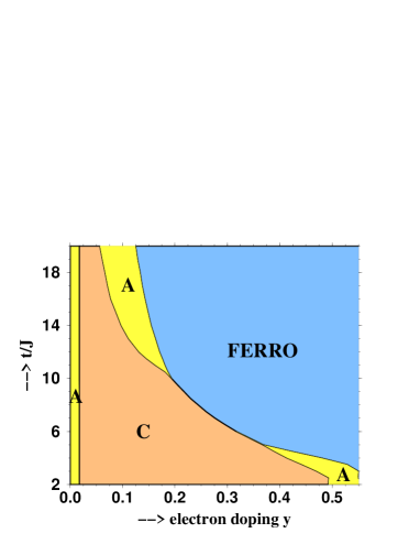
Figure 38: Phase diagram of the DE model with degenerate $e_{g}$ bands. Depending on the electron doping concentration and the ratio of the $e_{g}$ bandwidth and the $t_{2g}$ superexchange one finds either AF A-type (A), or C-type (C), or FM (FERRO) order (after Ref. Kho99 ).

VI.2 Spin-waves in a metallic phase

Unfortunately, the phase diagram shown in Fig. 38 does not allow to conclude anything about the favored magnetic phases near the filling of one $e_{g}$ electron per atom, i.e., in hole doped La_1-xSr_xMnO₃ with $x<0.5$, and other related compounds. In this case the $e_{g}$ electrons are strongly correlated and one cannot use the DE for degenerate orbitals as discussed in the previous Section. Due to strong on-site Coulomb interactions, the motion of $e_{g}$ electrons is then allowed only in the restricted space, without creating double occupancies which leads to the superexchange as explained in Sec. V.A. If a half-filled system is doped, the motion of holes in the $e_{g}$ band becomes possible when it is accompanied by a backflow of electrons which carry spin and orbital index. Thus, one has to consider a hopping problem which resembles the $t$-$J$ model. In order to make such a model realistic for doped manganites, the degeneracy of $e_{g}$ orbitals and the previously derived form of superexchange in the doped system (169) and (170) have to be included.

The problem of DE and the resulting phase diagram in the regime of hole doping belongs to the unsolved problems. The approximate solutions were presented by several groups Mae98 ; Kil99 ; Ish00 , but either the models were oversimplified, or only certain aspects of the phase diagram were treated. We shall discuss this problem in Sec. VIII; here we analyse only the FM metallic phase and show how the spin-waves follow from DE and superexchange magnetic interactions. Thus we consider an effective $t$-$J$ model for doped La_1-xA_xMnO₃ compounds in the FM regime Ole99 ,

$${\cal H}=H_{t}+H_{J}(e_{g})+H_{J}(t_{2g}),$$ (183)

where $H_{t}$ describes the correlated hopping in the $e_{g}$-band (38), with the operators $\hat{c}_{i\alpha\sigma}^{\dagger}$ which act in the projected space without double occupancies in $e_{g}$ orbitals, and $H_{J}(e_{g})$ and $H_{J}(t_{2g})$ stand for the SE terms (157) and (158), respectively.

The spectrum of magnetic excitations in FM phase is very important for a better understanding of the physics of manganites. Experimentally the spin-waves were measured by Perring et al. in La_0.7Pb_0.3MnO₃ Per96 along the main high-symmetry directions, and an isotropic dispersion was found. Similar observation were made by Endoh et al. in La_1-xSr_xMnO₃ End97 . They found out that unlike in localized FM systems, the energy of the spin-wave near the zone boundary is not approximately equal to $k_{B}T_{C}$, where $T_{C}$ is the Curie temperature, but is significantly larger. This can be interpreted as an experimental proof that the ferromagnetism in doped manganites is itinerant. However, the stiffness constant $D$ at low momenta is almost constant for different compounds at $x\simeq 0.3$ doping Fer98 . This universality is puzzling and suggests that a common mechanism is responsible in first place for the Goldstone modes and the spin dynamics at low momenta ${\vec{q}}$, while some other processes might be responsible for a much broader spectrum of the observed Curie temperatures $T_{C}$. First we will address the origin of spin-waves and show that the stiffness constant is approximately determined by the DE mechanism in a correlated $e_{g}$ band, $D\simeq J_{\text{DE}}S$, where $J_{\text{DE}}$ is the effective exchange constant which couples spins $S\simeq 2$. The corrections will come from superexchange which operates as well in doped systems and counteracts the DE mechanism.

In order to construct the spin excitations, we separate first the spin dynamics from charge and orbital dynamics. In reality all these processes which involve different degrees of freedom are coupled and are described by fermion operators $\hat{c}_{i\alpha\sigma}^{\dagger}$ in $H_{t}$. We represent such electron operators by fermion operators $\{f_{ix}^{\dagger},f_{iz}^{\dagger}\}$ which carry an orbital index, and by a Schwinger boson operator, either $a_{i\uparrow}^{\dagger}$ or $a_{i\downarrow}^{\dagger}$, depending on the spin $\sigma$ of the moving electron,

$$\hat{c}_{i\alpha\sigma}^{\dagger}=f_{i\alpha}^{\dagger}a_{i\sigma}^{\dagger}.$$ (184)

As in Sec. V.A, we use a local basis for the occupied $e_{g}$ orbitals: $|x\rangle\equiv|x^{2}-y^{2}\rangle$ and $|z\rangle\equiv|3z^{2}-r^{2}\rangle$. The decomposition (184) allows to simplify the MF analysis in the large-$U$ limit, where the Hilbert space contains only two kind of stated: Mn³⁺ $(d^{4})$ ions if a single $e_{g}$ electron is present, and Mn⁴⁺ $(d^{3})$ ions if an $e_{g}$ electron was removed. Formally this can be written using the configurations pm99 :

$$|i\theta,M\rangle_{4}=f_{ix}^{\dagger}b_{ix}^{\dagger}|M\rangle,\hskip 19.91684pt|i\epsilon,M\rangle_{4}=f_{iz}^{\dagger}b_{iz}^{\dagger}|M\rangle,\hskip 19.91684pt|i,m\rangle_{3}=b_{i0}^{\dagger}|m\rangle,$$ (185)

with $M$ being the component of spin $S=2$ for Mn³⁺ sites, and $m$ being the component of the core $t_{2g}$-spin $S=3/2$ for Mn⁴⁺ sites. The spin part is described by Schwinger bosons in a standard way Aue94 : $|M\rangle=(a_{i\uparrow}^{\dagger})^{S+M}(a_{i\downarrow})^{S-M}|0)$, where $|0)$ is the vacuum state, and similar for $|m\rangle$. The operators $b_{ix}^{\dagger}$ and $b_{iz}^{\dagger}$ in Eqs. (185) are slave boson operators which carry the orbital index and are introduced in order to restrict the physical space in analogy to the Kotliar-Ruckenstein bosons in the Hubbard model Kot86 . The empty boson $b_{i0}^{\dagger}$ counts Mn⁴⁺ ions and has a similar meaning. Using these boson operators we implement the local constraints,

$$a_{i\uparrow}^{\dagger}a_{i\uparrow}+a_{i\downarrow}^{\dagger}a_{i\downarrow}+b_{i0}^{\dagger}b_{i0} = 2S,$$ (186)

$$b_{ix}^{\dagger}b_{ix}+b_{iz}^{\dagger}b_{iz}+b_{i0}^{\dagger}b_{i0} = 1.$$ (187)

They restrict the physical space to contain no double occupancy in the $e_{g}$ orbitals. In addition, the number of fermions is equal to the number of bosons for each orbital, $f_{i\alpha}^{\dagger}f_{i\alpha}=b_{i\alpha}^{\dagger}b_{i\alpha}$, $\alpha=x,z$.

As a next step, we rewrite the hopping Hamiltonian $H_{t}$ assuming the FM metallic phase and derive the effective fermion problem with the constraints replaced by the operator expressions $z_{i\alpha}$ which contain the bosons used in Eq. (187) that accompany individual hopping processes in Eq. (38) pm99 ,

$$H_{t} = -\tilde{t}\sum_{\langle ij\rangle\perp,\sigma}a_{i\sigma}^{\dagger}z_{iz}^{\dagger}f_{iz}^{\dagger}f_{jz}z_{jz}a_{j\sigma}$$ (188)

$$- \frac{1}{4}\tilde{t}\sum_{\langle ij\rangle\parallel,\sigma}a_{i\sigma}^{\dagger}\left[3z_{ix}^{\dagger}f_{ix}^{\dagger}f_{jx}z_{jx}+z_{iz}^{\dagger}f_{iz}^{\dagger}f_{jz}z_{jz}\right.$$

$$\hskip 42.67912pt\left.\pm\sqrt{3}\left(z_{ix}^{\dagger}f_{ix}^{\dagger}f_{jz}z_{jz}+z_{iz}^{\dagger}f_{iz}^{\dagger}f_{jx}z_{jx}\right)\right]a_{j\sigma},$$

where the renormalized hopping $\tilde{t}$ is introduced in order to compensate for the extra factors resulting from the Schwinger boson operators, $\sim a_{i\sigma}^{\dagger}a_{j\sigma}$, when the kinetic energy is determined from $H_{t}$. The terms $z_{i\alpha}$ contain the orbital bosons $b_{i\alpha}^{\dagger}$ and an empty boson $b_{i0}^{\dagger}$, and are similar to the respective factors $z_{i\sigma}$ used in the spin problem Kot86 . The first sum includes the bonds $\langle ij\rangle\perp$ along the $c$-axis, while the second sum includes the bonds $\langle ij\rangle\parallel$ within the $(a,b)$ planes. The MF theory is constructed by averaging over the orbital and empty bosons, and one finds the simpler form of the hopping Hamiltonian,

$$H_{t} = -\tilde{t}\sum_{\langle ij\rangle\perp,\sigma}a_{i\sigma}^{\dagger}q_{iz}^{*}f_{iz}^{\dagger}f_{jz}q_{jz}a_{j\sigma}$$ (189)

$$-\frac{1}{4}\tilde{t}\sum_{\langle ij\rangle\parallel,\sigma}a_{i\sigma}^{\dagger}\left[3q_{ix}^{*}f_{ix}^{\dagger}f_{jx}q_{jx}+q_{iz}^{*}f_{iz}^{\dagger}f_{jz}q_{jz}\right.$$

$$\hskip 42.67912pt\left.\pm\sqrt{3}\left(q_{ix}^{*}f_{ix}^{\dagger}f_{jz}q_{jz}+q_{iz}^{*}f_{iz}^{\dagger}f_{jx}q_{jx}\right)\right]a_{j\sigma},$$

where the renormalization factors at site $i$ ($x=1-n$),

$$q_{ix}=\left(\frac{2x}{1+x+(1-x)\cos 2\theta_{i}}\right)^{1/2},\hskip 19.91684ptq_{iz}=\left(\frac{2x}{1+x-(1-x)\cos 2\theta_{i}}\right)^{1/2},$$ (190)

depend on the angle $\theta_{i}$ which defines the occupied orbital state (65). In the FM state we assume that the orbitals are homogeneous, and the angles correspond to an average orbital state, $\theta_{i}=\theta$.

Now we consider the Schwinger boson operators in Eq. (189). At low temperatures the magnetic moment of FM metallic manganites is almost fully saturated. It is therefore reasonable to expand Eq. (189) around a FM ground state. Technically this is done by condensing the spin-up Schwinger bosons $a_{i\uparrow}\simeq\sqrt{2\bar{S}}$ (if the magnetic moments point upwards), and by treating the spin-down Schwinger bosons in leading order of $1/\bar{S}$ expansion to describe spin-wave excitations around this ground state. Assuming that the spins are pointing upwards in the MF state, we derive from the constraint (186) the following expansion of the $a_{i\uparrow}^{\dagger}$-bosons pm99 ,

$$a_{i\uparrow}=\sqrt{2\bar{S}-a_{i\downarrow}^{\dagger}a_{i\downarrow}}\simeq\sqrt{2\bar{S}}\left(1-\frac{1}{4\bar{S}}a^{\dagger}_{i\downarrow}a_{i\downarrow}\right),$$ (191)

where the effective spin $2\bar{S}=2S-x$ is defined using the MF state in Eq. (186), with $\langle b_{i0}^{\dagger}b_{i0}\rangle=x$. We see that the extra factor generated by Schwinger bosons is equal $2\bar{S}$, and thus one has to use $\tilde{t}=t/2\bar{S}$ in Eq. (188). The final form of the hopping Hamiltonian in the correlated $e_{g}$ band is obtained after replacing the Schwinger bosons by Holstein-Primakoff boson operators $a_{i}$. As the expansion (191) is performed around the FM state, we use therefore $a_{i\downarrow}\equiv a_{i}$ to study the fluctuations,

$$\sum_{\sigma}a_{i\sigma}^{\dagger}a_{j\sigma}\simeq 2\bar{S}-\frac{1}{2}\left(a_{i}^{\dagger}a_{i}+a_{j}^{\dagger}a_{j}-2a_{i}^{\dagger}a_{j}\right).$$ (192)

This expansion leads to the following form of the kinetic energy term,

$$H_{t}=-\sum_{\langle ij\rangle\alpha\beta}t_{ij}^{\alpha\beta}q_{i\alpha}q_{j\beta}f_{i\alpha}^{\dagger}f_{j\beta}+\frac{1}{4\bar{S}}\sum_{\langle ij\rangle\alpha\beta}t_{ij}^{\alpha\beta}q_{i\alpha}q_{j\beta}f_{i\alpha}^{\dagger}f_{j\beta}\Big{(}a_{i}^{\dagger}a_{i}+a_{i}^{\dagger}a_{i}-2a_{i}^{\dagger}a_{j}\Big{)}.$$ (193)

Consider first the zeroth-order Hamiltonian,

$$H_{t}^{(0)}=-\sum_{\langle ij\rangle\alpha\beta}t_{ij}^{\alpha\beta}q_{i\alpha}q_{j\beta}f_{i\alpha}^{\dagger}f_{j\beta}.$$ (194)

It describes the orbital model with correlated fermions; the hopping amplitudes $\propto t_{ij}^{\alpha\beta}q_{i\alpha}q_{j\beta}$ depend on the actual shape of occupied $e_{g}$ orbitals Fei00 . This problem was studied qualitatively by van Veenendaal and Fedro Vee99 who pointed out that the asymmetry in the magnetic phase diagrams of doped manganites between $x>0.5$ and $x<0.5$ doping follows from the essentially uncorrelated electrons in the former, and strongly correlated electrons that avoid each other in the latter case. The correlations cause strong band narrowing in the regime of $x\to 0$ due to the reduction of the hopping elements by the $q_{ix}$ and $q_{iz}$ factors in Eq. (190). One finds that the correlated band structure is drastically reduced in the disordered states with $\cos 2\theta=0$, while smaller reductions are found when the occupied orbitals are close to either $|x\rangle$ or $|z\rangle$ states (Fig. 39). By this mechanism one finds a tendency towards an orbital liquid state as observed by Ishihara, Yamanaka and Nagaosa Nag97 . Such a symmetry breaking in the orbital space happens easily in a 2D case, where the kinetic energy drives the system into the phase with $|x\rangle$ orbitals occupied Mac99 , while there are also other possibilities to stabilize a disordered state in three dimensions Fei00 , and thus the orbital liquid of this type is unlikely.

The orbital model (194) in the limit of $U\to\infty$ is equivalent to the spinless fermion problem. The band structure collapses at $n=1$ to a line at $\omega=0$, and the kinetic energy vanishes. In analogy to the Hubbard model in $U\to\infty$ limit, the kinetic energy, $E_{\rm kin}=\langle H_{t}^{(0)}\rangle$, is symmetric with respect to the filling of $n=0.5$, i.e., the system gains kinetic energy at increasing hole concentration in the regime of $0<x<0.5$ ($1.0>n>0.5$) (Fig. 40). In contrast, free $e_{g}$ electrons would give a metallic behavior with the largest kinetic energy near $n=1$. This demonstrates that the correlations due to the orbital degree of freedom have to be explicitly included in order to reproduce the insulating state in the limit of $x\to 0$.

Figure 39: Correlated band structure as obtained for two densities of $e_{g}$ electrons: (a) $n=0.99$, and (b) $n=0.70$, in the FM disordered state with the same electron density in both $e_{g}$ orbitals, $\langle n_{x}\rangle=\langle n_{z}\rangle=n/2$ (full lines), and for the fully polarized orbital liquid state Nag97 with $\langle n_{x}\rangle=n$ (dashed lines) (after Ref. Fei00 ).

Figure 40: Kinetic energy as a function of $e_{g}$ band filling $n$ for the correlated (194) (solid line) and uncorrelated (173) electrons (dashed line) (after Ref. Fei00 ).

After studying DE in degenerate $e_{g}$ orbitals (Sec. VI.A), it might be expected that this mechanism produces in first instance anisotropic magnetic phases, such as A-AF and C-AF states. However, these solutions are de facto stabilized really by the superexchange interactions in Ref. Bri99 . However, we have shown in Sec. V.A (see Table 2) that the realistic superexchange constants are much smaller that the hopping element $t$, and thus the magnetic properties in the highly doped regime are determined primarily by the DE term (194). Consequently, it is allowed to assume that the ground state is FM, and to expand around this state which leads to the DE part of the spin dynamics described by the first order term in Eq. (193) when the orbital and charge dynamics are averaged out,

$$H_{t}^{(1)}\simeq\frac{1}{4\bar{S}}\sum_{\langle ij\rangle\alpha\beta}t_{ij}^{\alpha\beta}q_{i\alpha}q_{j\beta}\langle f_{i\alpha}^{\dagger}f_{j\beta}\rangle\Big{(}a_{i}^{\dagger}a_{i}+a_{i}^{\dagger}a_{i}-2a_{i}^{\dagger}a_{j}\Big{)}.$$ (195)

Using the renormalization factors for the correlated band structure (190), this averaging yields the magnon dispersion due to the DE mechanism pm99 ,

$$\omega_{\vec{q}}=\frac{t}{2\bar{S}}\left(2[1-\gamma_{+}({\vec{q}})]R_{ab}+[1-\gamma_{z}({\vec{q}})]R_{c}\right),$$ (196)

where $\gamma_{+}({\vec{q}})$ and $\gamma_{z}({\vec{q}})$ are defined by Eqs. (106) and (108), respectively, and $t=0.40$ eV is the largest local hopping element between two $3z^{2}-r^{2}$ orbitals along the $c$-axis Fei99 . The lattice sums $R_{ab}$ and $R_{c}$ can be easily derived and depend on the average occupancy of $|x\rangle$ and $|z\rangle$ orbitals, $n_{x}$ and $n_{z}$.

For a disordered state represented by the orbitals with complex coefficients Fei00 , and $\cos 2\theta=n_{x}-n_{z}=0$, the Gutzwiller renormalization factors (190) become equal, $q_{ix}=q_{iz}=q$, and it is convenient to express the result as,

$$\omega_{\vec{q}}=zJ_{\rm DE}\bar{S}(1-\gamma_{\vec{q}}),$$ (197)

with $\gamma_{\vec{q}}$ defined as in Eq. (32), $z=6$, and the effective FM exchange constant determined by the kinetic energy of correlated electrons,

$$J_{\rm DE}=\frac{tq^{2}}{2\bar{S}^{2}}\,\frac{1}{N}\sum_{{\vec{k}}\nu}\langle f_{{\vec{k}}\nu}^{\dagger}f_{{\vec{k}}\nu}\rangle\cos k_{\alpha}.$$ (198)

The summation in Eq. (198) runs over the occupied band states in each subband $\nu$, and the band structure of degenerate $e_{g}$ orbitals (178) is renormalized by $q^{2}=2x/(1+x)$. It gives the same result for any cubic direction $\alpha=a,b,c$, so only one component $\propto\cos k_{\alpha}$ was included. Thus, one finds isotropic spin-waves with the spin-wave stiffness constant $D=J_{\rm DE}\bar{S}$. The qualitative result of the Kondo lattice model with a nondegenerate band Fur96 is therefore reproduced in the correlated $e_{g}$ band. The advantage is that the present approach pm99 is more straightforward and may be directly used to study the corrections of the DE result due to the superexchange terms (169) and (170). Both superexchange terms may be expanded using Schwinger bosons around the FM state and lead to an isotropic reduction of the effective FM DE interactions, if a disordered orbital state with $\langle{\cal P}_{\langle ij\rangle}^{\zeta\xi}\rangle=1/2$ and $\langle{\cal P}_{\langle ij\rangle}^{\zeta\zeta}\rangle=1/2$ is considered. Under these circumstances, the $e_{g}$ superexchange (169) is isotropic and weakly AF, taking the parameters $U=7.3$ eV and $J_{H}=0.69$ eV, as given in Sec. V.A. The second AF term comes from the $t_{2g}$ superexchange (170), with the constants $J_{t}=2.1$ meV, ${\hat{J}}_{t}=4.6$ meV, and ${\bar{J}}_{t}=5.5$ meV for the pairs of Mn³⁺–Mn³⁺, Mn⁴⁺–Mn⁴⁺, and Mn³⁺–Mn⁴⁺ ions, respectively (see Sec. V.B).

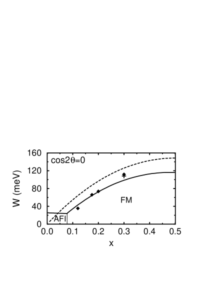
Figure 41: Width $W$ of the magnon dispersion in FM manganites La_1-xA_xMnO₃ as a function of doping $x$, as obtained including only the DE mechanism (197) (dashed line), and both DE and superexchange contributions (full line). In the AF insulating (AFI) phase at $x<0.08$ only the anisotropic superexchange interactions contribute. Experimental points correspond to: La_1-xSr_xMnO₃ End97 (diamonds) and La_0.7Pb_0.3MnO₃ Per96 (cross) (after Ref. pm99 ).

If hole doping $x$ increases, first the A-AF insulating (AFI) state is modified as reported in Sec. V.B. In this regime the superexchange dominates over the DE term, and a different expansion around the A-AF phase with the polaronic FM superexchange (172) has to be used to derive the spin-waves (Sec. V.B). We present the numerical result for the total magnon width $W$ obtained by these different approaches for the AFI and FM phases in Fig. 41. The theory predicts an observed increase of the magnon width $W$ with increasing doping $x$ pm99 due to the DE which dominates in the metallic regime of $x>0.08$. The DE contribution to $W$ vanishes in the $x\to 0$ limit, in contrast to the unphysical result of band structure calculations that ignore electron correlations, and give the largest FM interactions at $x=0$ Sol99 , precisely at the point where the A-AF ordering in insulating LaMnO₃ is observed.

The magnon dispersion is isotropic if the orbitals are disordered. We emphasize that orbital ordering leads instead to anisotropic magnon dispersion, and therefore such states as obtained recently by Okamoto, Ishihara and Maekawa Ish00 would lead to anisotropic spin-wave dispersions not only in the A-AF phase, but also in the FM regime. The quality of the model may be best appreciated by an excellent agreement with the experimental results for $x=0.3$ doped manganite La_0.7Pb_0.3MnO₃ Per96 . The exchange interactions found in Ref. pm99 at $x=0.3$: $J_{ab}\bar{S}=J_{c}\bar{S}=8.24$ meV are isotropic and reproduce very well the experimental points (Fig. 42). In conclusion, the magnon dispersion derived from DE for degenerate $e_{g}$ orbitals supplemented by smaller superexchange terms agrees well with the experimental findings in FM metallic manganites Per96 ; End97 .

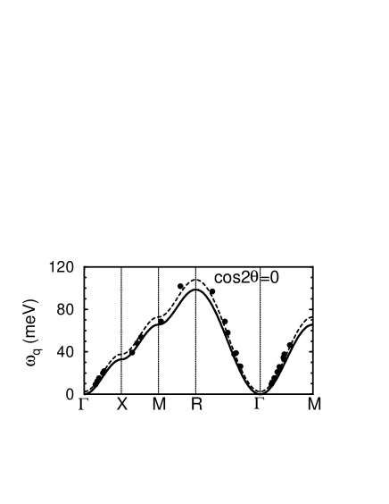
Figure 42: Magnon dispersion $\omega_{\bf q}$ as obtained at $x=0.3$ doping using DE and superexchange contributions (heavy line); parameters as in Ref. Fei99 . Experimental data for La_0.7Pb_0.3MnO₃ (circles and dashed line) are reproduced from Ref. Per96 (after Ref. pm99 ).

VI.3 Magnon softening in ferromagnetic manganites

One of the puzzling features is nonuniversality of the magnetic and transport properties of FM manganites at doping $x\simeq 0.30$ End97 . As we have shown in Sec. VI.B, the spin-wave dispersion which follows from the DE model for correlated $e_{g}$ electrons (197) is isotropic in all three cubic directions and of the nearest-neighbor Heisenberg type. Recently, unexpected deviations from this dispersion with a peculiar softening of the magnon spectrum close to the magnetic zone boundary has experimentally been observed in compounds with low values of $T_{C}$. Quite prominent in this respect are measurements of the spin dynamics of the FM manganese oxide Pr_0.63Sr_0.37MnO₃ Hwa98 . While exhibiting conventional Heisenberg behavior at small momenta, the magnetic excitations soften at the boundary of the BZ. Assuming the magnon dispersion to be of Heisenberg type with an exchange constant $J_{eff}$, the dispersion is quadratic in the regime of ${\vec{q}}\simeq 0$, $\omega_{\vec{q}}\simeq Dq^{2}$, with the spin-wave stiffness $D\propto J_{eff}$. Since the latter also controls the Curie temperature $T_{C}\propto J_{eff}$, the ratio of $D$ and $T_{C}$ is expected to be a universal constant. Manganites, however, exhibit a pronounced deviation from this behavior: $D/T_{C}$ increases significantly as one goes from compounds with high to compounds with low values of $T_{C}$ Fer98 . This feature together with the above magnon softening at the magnetic zone boundary indicate that the DE model does not suffice and some specific feature of magnetism in manganites has not yet been identified.

Here we report shortly an interesting recent proposal by Khaliullin and Kilian Kha00 that charge and coupled orbital-lattice fluctuations are responsible for the unusual magnon softening. The starting point is not the $t$-$J$ model for manganites (183), but a Kondo lattice model with orbital degeneracy which is a generalization of the DE model (23) and takes into account the correlated nature of $e_{g}$ electrons. We begin by analyzing the DE part,

$$H=-\sum_{\langle ij\rangle\alpha\beta\sigma}t_{ij}^{\alpha\beta}\Big{(}\hat{c}^{\dagger}_{i\alpha\sigma}\hat{c}_{j\beta\sigma}+H.c.\Big{)}-J_{H}\sum_{i\alpha\sigma\sigma{{}^{\prime}}}{\vec{S}}_{i}\cdot c_{i\alpha\sigma}^{\dagger}\vec{\sigma}_{\sigma\sigma{{}^{\prime}}}c_{i\alpha\sigma{{}^{\prime}}},$$ (199)

where the constrained operators $\hat{c}^{\dagger}_{i\alpha\sigma}$ act in the projected space without double occupancies in the $e_{g}$ orbitals, as in Eq. (183). Due to the strong Hund’s coupling $\propto J_{H}$, core spins ${\vec{S}}_{i}$ and itinerant $e_{g}$ spins ${\vec{s}}_{i}$ are not independent of each other; rather a high-spin state with total on-site spin $S=S_{t}+\frac{1}{2}$, where $S_{t}=3/2$, is formed. This unification of band and local spin subspaces suggests to decompose the $e_{g}$ electron into its spin and orbital/charge components. As we have shown in Sec. VI.B following Ref. pm99 , the $e_{g}$ spin can then be absorbed into the total spin, allowing an independent treatment of spin and orbital/charge degrees of freedom. The formal procedure which allows for this separation scheme is realized by introducing Schwinger bosons $d_{i\uparrow}$ and $d_{i\downarrow}$ to describe the $e_{g}$ spin subspace,

$$s_{i}^{+}=d^{\dagger}_{i\uparrow}d_{i\downarrow},\hskip 19.91684pts_{i}^{-}=d^{\dagger}_{i\downarrow}d_{i\uparrow},\hskip 19.91684pts_{i}^{z}=\frac{1}{2}(d^{\dagger}_{i\uparrow}d_{i\uparrow}-d^{\dagger}_{i\downarrow}d_{i\downarrow}),$$ (200)

as well as Schwinger bosons $a^{\dagger}_{i\uparrow}$ and $a^{\dagger}_{i\downarrow}$ to model the total on-site spin $S=2$,

$$S_{i}^{+}=a^{\dagger}_{i\uparrow}a_{i\downarrow},\hskip 19.91684ptS_{i}^{-}=a^{\dagger}_{i\downarrow}a_{i\uparrow},\hskip 19.91684ptS_{i}^{z}=\frac{1}{2}(a^{\dagger}_{i\uparrow}a_{i\uparrow}-a^{\dagger}_{i\downarrow}a_{i\downarrow}).$$ (201)

These auxiliary particles are subject to the following constraints that depend on the $e_{g}$ occupation number $n_{i}$:

$$d^{\dagger}_{i\uparrow}d_{i\uparrow}+d^{\dagger}_{i\downarrow}d_{i\downarrow} = n_{i},$$ (202)

$$a^{\dagger}_{i\uparrow}a_{i\uparrow}+a^{\dagger}_{i\downarrow}a_{i\downarrow} = 2S-1+n_{i}.$$ (203)

This is in fact a different way of writing the constraints (186) and (187). By construction, one assumes in both approaches that high-spin states $S=2$ are realized at the sites occupied by $e_{g}$ electrons which corresponds to the large $J_{H}$ limit. The creation and annihilation operators for $e_{g}$ electrons can then be expressed in terms of spinless fermions $f_{i\alpha}^{\dagger}$ which carry charge and orbital pseudospin and Schwinger bosons which carry spin in analogy to Eq. (184),

$$\hat{c}_{i\alpha\sigma}^{\dagger}=\hat{c}_{i\alpha}^{\dagger}d_{i\sigma}^{\dagger}.$$ (204)

The Bose operators are subject to the constraint (202) that enforces the operators $d_{i\sigma}$ and $d^{\dagger}_{i\sigma}$ to act only in the projected Hilbert space with one or zero Schwinger bosons, respectively. Our aim is to absorb the $e_{g}$ spin into the total spin, which requires to map the $e_{g}$ operators $d_{i\sigma}$ onto the operators $a_{i\sigma}$ for the total spin. It is easy to obtain the following mapping

$$d_{i\sigma}=\frac{1}{\sqrt{2S}}a_{i\sigma}.$$ (205)

The kinetic energy in Hamiltonian (199) now describes the simultaneous transfer of pairs of spinless fermions and Schwinger bosons, and can be rewritten in the form analogous to Eq. (189). However, one can still use the fermion operators which carry the orbital index, unlike in Sec. VI.B, where orbital bosons were introduced as well in Eq. (189). One finds,

$$H_{t}=-\frac{1}{2S}\sum_{\langle ij\rangle\alpha\beta\sigma}t_{ij}^{\alpha\beta}\left(\hat{c}^{\dagger}_{i\alpha}\hat{c}_{j\beta}a^{\dagger}_{i\sigma}a_{j\sigma}+H.c.\right),$$ (206)

Thus, the above consideration provides a formal proof that the above construction with two Schwinger bosons $d_{i\sigma}$ and $a_{i\sigma}$ Kha00 is completely equivalent to introducing only one type of Schwinger bosons referring to the total spins $S=2$ Ole00 , as shown in Sec. V.B. One finds therefore the same expansion of the kinetic energy as given by Eq. (193), except that the Kotliar-Ruckenstein bosons have not yet been introduced in the present case (206), and one may therefore study the renormalization of magnons by quantum fluctuations beyond the MF theory.

To study the propagation of the magnetic excitations in hole-doped DE systems, we now derive first the correct spin operator taking into account the fact that the total on-site spin depends on whether a hole or an $e_{g}$ electron is present at that site. The spin quantum number is $S-\frac{1}{2}$ in the former and $S$ in the latter case. In general, a spin excitation is created by the operator $S_{i}^{+}$. Expressing this operator in terms of Schwinger bosons $S^{+}_{i}=a^{\dagger}_{i\uparrow}a_{i\downarrow}$, and next condensing $a_{i\uparrow}$ and mapping $a_{i\downarrow}$ onto the magnon annihilation operator $a_{i}$ as in Sec. V.B, the following representation is obtained,

$$S^{+}_{i}=\left\{\begin{array}[]{ll}\displaystyle\sqrt{2S}\;a_{i},&\text{for sites with $e_{g}$ electron},\\ \displaystyle\sqrt{2S-1}\;a_{i},&\text{for sites with hole}.\end{array}\right.$$

Assuming $S$ to be the “natural” spin number of the system, the magnon operator $a_{i}$ hence has to be rescaled by a factor $[(2S-1)/(2S)]^{1/2}$ when being applied to hole sites,

$$A_{i}=\left\{\begin{array}[]{ll}\displaystyle a_{i},&\text{for sites with $e_{g}$ electron},\\ \displaystyle\sqrt{(2S-1)/(2S)}\;a_{i},&\text{for sites with hole}.\end{array}\right.$$

The general magnon operator $A_{i}$ that automatically probes the presence of an $e_{g}$ electron can finally be written as

$$A_{i}=a_{i}\Bigg{[}n_{i}+\sqrt{\frac{2S-1}{2S}}(1-n_{i})\Bigg{]}\approx a_{i}-\frac{1}{4S}(1-n_{i})\;b_{i},$$ (207)

where $n_{i}$ is the number operator of $e_{g}$ electrons at site $i$. It turns out that $A_{i}$ represents the true Goldstone operator of hole-doped DE systems. Its composite character comprises local and itinerant spin features which is a consequence of the fact that static core and mobile $e_{g}$ electrons together build the total on-site spin. While the itinerant part of $A_{i}$ is of order $1/S$ only, it nevertheless is of crucial importance to ensure consistency of the spin dynamics with the Goldstone theorem, i.e., to yield an excitation mode whose energy vanishes at zero momentum Kha00 .

Having derived the correct magnon operators $A_{i}$ for doped DE systems (207) allows to study the energies of magnetic excitations, and their renormalization caused by the coupling of magnons to other quasiparticles present in the correlated $e_{g}$ band, and the coupling to the lattice. If such processes are neglected, one finds the magnon dispersion determined primarily by the DE in a strongly correlated $e_{g}$ band, as shown in Sec. VI.B. If, however, the fermion and orbital variables are not averaged out, dynamical processes become possible which dress the magnons and result in finite selfenergy $\Sigma(\omega,{\vec{q}})$. Therefore, the magnon spectrum in an interacting system $\tilde{\omega}_{\vec{p}}$ contains the many-body correction expressed by the magnon selfenergy,

$$\tilde{\omega}_{\vec{q}}=\omega_{\vec{q}}+\text{Re}[\Sigma(\omega_{\vec{q}},{\vec{q}})].$$ (208)

The MF magnon dispersion $\omega_{\vec{q}}$ is of conventional nearest-neighbor Heisenberg form (197), and we have seen in Sec. VI.B that it gives the spin-wave stiffness constant $D=J_{\text{DE}}S$.

Apart from electron dynamics in the correlated $e_{g}$ orbitals which is treated by the projected operators $\hat{c}^{\dagger}_{i\alpha}$, virtual charge-transfer processes across the Hubbard gap contribute to the superexchange. At low and intermediate doping levels the superexchange due to the hopping of $e_{g}$ electrons is of importance, and this contributes with a FM component as the high-spin state gives the only nonvanishing magnetic term, if electrons are polarized. These superexchange processes $\propto J_{\text{SE}}$ establish an intersite interaction, which in the limit of a strong Hund’s coupling could be written in the form Kha00 ,

$$H_{J}=-J_{\text{SE}}\sum_{\langle ij\rangle}\left(\frac{1}{4}-\tau_{i}^{\alpha}\tau_{j}^{\alpha}\right)\left[{\vec{S}}_{i}{\vec{S}}_{j}+S(S+1)\right]n_{i}n_{j}.$$ (209)

Thus one might naively expect that the stiffness constant $D$ is increased by the superexchange $J_{\text{SE}}$ which thus amplifies the DE effect $\propto J_{\text{DE}}$ in the correlated $e_{g}$ band, resulting in $D\propto J_{\text{DE}}+J_{\text{SE}}$ Kha00 . While the FM term is the only term which contributes in the ground state, the situation is different in the excited states and the above simplified picture is incorrect. It has been shown in Sec. VI.B that the DE effect is reduced by superexchange interactions. The reason is twofold: (i) a few AF interactions are generated by the effective processes which involve $e_{g}$ electrons (157), and they have to be included for the realistic parameters with finite $J_{H}$ (and not using $J_{H}=\infty$), and (ii) the processes which involve $t_{2g}$ electrons contribute as well with AF superexchange terms (170). Therefore, the AF superexchange due to both $e_{g}$ and $t_{2g}$ electrons always dominates over a single FM $e_{g}$ contribution, and thus the total superexchange decreases the stiffness constant and de facto counteracts the DE in the FM manganites.

Fortunately, the above incorrect interpretation of Ref. Kha00 is of quantitative nature and one may still use the same expansion of the DE processes around the FM state in order to study the consequences of magnon interactions with orbital excitations and with the lattice. Using the slave formalism similar to that introduced in Sec. VI.B, Khaliullin and Kilian derived the effective processes which describe the coupling of magnons to charge and orbital fluctuations separately Kha00 . These processes involve always scattering of either charge (fermionic) or orbital (bosonic) states on the magnons, and lead in lowest order to the contributions to the magnon selfenergy $\Sigma(\omega,{\vec{q}})$ shown in Figs. 43(a) and 43(b).

The softening of magnons at the zone boundary was observed in Pr_0.63Sr_0.37MnO₃, the compound which has a lower value of $T_{C}$ Hwa98 , while no softening was found earlier in metallic La_0.7Pb_0.3MnO₃ Per96 . The compounds with lower values of $T_{C}$ are worse metals and become in some cases insulating Fer98 , as for instance Pr_1-xCa_xMnO₃. This suggests that the lattice degrees of freedom are likely to play an important role in the magnon softening. The crystal dynamics is given by the Hamiltonian,

$$H_{\rm ph}=\frac{1}{2}K\sum_{i}{\vec{Q}}_{i}^{2}+K_{1}\sum_{\langle ij\rangle}Q_{i}^{\alpha}Q_{j}^{\alpha}+\frac{1}{2M}\sum_{i}{\vec{P}}_{i}^{2},$$ (210)

where ${\vec{Q}}_{i}=(Q_{2i},Q_{3i})$, $Q_{i}^{a(b)}=(Q_{3i}\pm\sqrt{3}Q_{2i})/2$, $Q_{i}^{c}=Q_{3i}$, and $Q_{2i}$ and $Q_{3i}$ are JT phonons of Fig. 3. The coupling of the spin-waves to phonons depends on the ratio $k_{1}=K_{1}/K$.

One of the central results of Ref. Kha00 is that the coupling between spins and phonons is indirect – it is mediated via the orbital channel. Orbital fluctuations couple to the spins be the DE term (206), while the coupling of orbitals to phonons (7) admixes low phononic frequencies into orbital fluctuations. The corresponding effective spin-phonon interaction is of the form,

$$H_{\rm s-ph}=\sum_{{\vec{p}}{\vec{q}}\lambda}g_{{\vec{p}}{\vec{q}}}^{\lambda}(b_{{\vec{q}}\lambda}^{\dagger}+b_{-{\vec{q}}\lambda})A_{\vec{p}}^{\dagger}A_{{\vec{p}}+{\vec{q}}},$$ (211)

where $b_{{\vec{q}}\lambda}^{\dagger}$ are the phonon creation operators for the mode $\lambda=1,2$ with momentum ${\vec{q}}$, $A_{\vec{p}}^{\dagger}$ are the Fourier transforms of the boson operators $A_{i}$ (207), and $g_{{\vec{p}}{\vec{q}}}^{\lambda}$ are the respective coupling constants which depend on the frequency of the involved phonon mode.

(a)

(b)

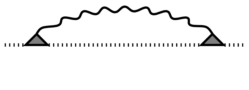
(c)

Figure 43: Magnon selfenergies describing the effect of magnon scattering on (a) orbital fluctuations, (b) charge fluctuations, and (c) phonons. Solid, dashed, dotted, and wiggled lines denote orbiton, holon, magnon, and phonon propagators, respectively (after Ref. Kha00 ).

The corresponding diagram which contributes to the magnon selfenergy is shown in Fig. 43(c). Using perturbation theory, different processes shown in Fig. 43 lead to the expressions which contain summations over internal momenta. Such summations were performed numerically using a Monte-Carlo algorithm in Ref. Kha00 and give the result shown by solid lines in Fig. 44. We note that the bare MF dispersion $\omega_{\vec{p}}$ is somewhat overestimated for the chosen parameters, as the contributions coming from the AF superexchange were neglected Kha00 . Therefore, the good agreement with experiment claimed for the stiffness constant $D$ using the spectroscopic value of $t=0.4$ eV Boc96 is fortuitous; in fact it implies that the value of $t$ is somewhat different in Pr_0.63Sr_0.37MnO₃ from the above value which gives a very good agreement for the stiffness constant in La_0.7Pb_0.3MnO₃ when the superexchange contributions are correctly included pm99 . It is clear, however, that the experimental magnon dispersion can be reproduced by Eq. (208) in the parameter space of the model which includes the coupling to the lattice (211). In the actual calculation, with the result shown in Fig. 44 Kha00 , the phonon contribution was determined using: $E_{\text{JT}}a_{0}^{2}\equiv(g_{2}a_{0})^{2}/2K=0.004$ eV, $\omega_{0}=0.08$ eV Oki95 , and $\Gamma=0.04$ eV. More details may be found in Ref. Kha00 .

As the main result, a pronounced softening of magnons at large momenta can be reproduced in the theory which treats the coupling of spin waves to the fluctuations of the orbital and lattice degrees of freedom Kha00 . Interestingly, charge fluctuations are found to play only a minor role. This follows qualitatively from the energy scales – the spectral density of charge fluctuations $\propto U$ lies well above the magnon band. In contrast, orbital and lattice fluctuations have rather low characteristic frequencies ($\propto xt$ and $\propto\omega_{0}$, respectively) and hence may couple stronger to spin-waves. The precise mechanism of this coupling is not yet completely understood, however. The numerical study of Ref. Kha00 suggests that the presence of JT phonons amplifies the magnon softening which follows in first instance from orbital fluctuations. The softening at the zone boundary, which occurs simultaneously with practically unaffected spin dynamics at small momenta that enters the spin-wave stiffness $D$ Fer98 , indicates that the instability towards an orbital-lattice ordered state is responsible for this phenomenon. The unusual magnon dispersion experimentally observed in low-$T_{C}$ manganites Hwa98 can hence be understood as a precursor effect of orbital-lattice ordering.

Figure 44: Magnon dispersion along $(0,0,\xi)$, $(\xi,\xi,0)$, and $(\xi,\xi,\xi)$ directions, where $\xi=0.5$ is at the cubic zone boundary. Experimental data from Ref. Hwa98 are indicated by circles, the MF dispersion $\omega_{\vec{q}}$ is marked by dashed lines. Solid lines represent the theoretical result for the dispersion $\tilde{\omega}_{\vec{q}}$ defined by Eq. (208); it includes charge, orbital, and lattice effects. The upper curve is obtained for dispersionless phonons with $k_{1}=0$, the lower one is a fit to the experimental data with $k_{1}=-0.33$ corresponding to ferrotype orbital-lattice correlations (after Ref. Kha00 ).

VII Orbital degrees of freedom in a ferromagnet

VII.1 Orbital excitations

While the electronic interactions in cuprates might stabilize a spin liquid in particular situations (Sec. IV), the spin-orbital model in manganites is in the opposite limit. Large Hund’s rule interactions $\propto J_{H}$ stabilize the orbital ordered states at the filling of one $e_{g}$ electron per site and at low doping, and FM planes stagger in the A-AF phase. Thus, the spin degree of freedom can be integrated out and one is left with orbital dynamics. In the undoped case one finds an anisotropic pseudospin model with an interesting behavior, as the pseudospin quantum number is not conserved vdB99 .

The proper understanding of pure orbital excitations is very important, both for fundamental reasons, and as a starting point to consider weakly doped FM $(a,b)$ planes of La_1-xA_xMnO₃. Therefore, we consider an idealized uniform FM phase. In this case the only superexchange channel which contributes is the effective interaction via the high-spin state, and one finds the effective Hamiltonian which describes $e_{g}$ electrons in a cubic crystal at strong-coupling Fei97 ; Ish97 ; Shi97 ,

$${\cal H}=H_{J}(e_{g})+H_{\tau}.$$ (212)

It consists of the superexchange part $H_{J}(e_{g})$, and the orbital splitting term due to crystal-field term $H_{\tau}$ (59) which is connected with the uniaxial pressure and was introduced before in Sec. III.A. An example of such a model is the superexchange interaction in the FM state of LaMnO₃ which originates from $d_{i}^{4}d_{j}^{4}\rightleftharpoons d_{i}^{3}d_{j}^{5}$ excitations into a high-spin $d_{j}^{5}$ state $|^{6}\!A_{1}\rangle$ (with $d_{i}^{4}\equiv t_{2g}^{3}e_{g}$, $d_{i}^{3}\equiv t_{2g}^{3}$, and $d_{i}^{5}\equiv t_{2g}^{3}e_{g}^{2}$). It gives the effective Hamiltonian with orbital interactions,

$$H_{J}(e_{g})=-\frac{t^{2}}{\varepsilon(^{6}\!A_{1})}\sum_{\langle ij\rangle}{\cal P}_{\langle ij\rangle}^{\zeta\xi},$$ (213)

where $t$ is the hopping element between the directional $3z^{2}-r^{2}$ orbitals along the $c$-axis, and $\varepsilon(^{6}\!A_{1})$ is the excitation energy Fei99 . The orbital degrees of freedom are described by the projection operators ${\cal P}_{\langle ij\rangle}^{\zeta\xi}$ (61) which select a pair of orbitals $|\zeta\rangle$ and $|\xi\rangle$, being parallel and orthogonal to the directions of the considered bond $\langle ij\rangle$ in a cubic lattice.

The Hamiltonian (213) has cubic symmetry and may be written using any reference basis in the $e_{g}$ subspace. For the conventional choice of $|x\rangle$ and $|z\rangle$ orbitals, the above projection operators ${\cal P}_{\langle ij\rangle}^{\zeta\xi}$ are represented by the orbital operators $\tau_{i}^{\alpha}$, with $\alpha=a,b,c$ for three cubic axes, defined by Eqs. (49) and (50). We replace them by pseudospin operators $T^{x}_{i}=\frac{1}{2}\sigma^{x}_{i}$ and $T^{z}_{i}=\frac{1}{2}\sigma^{z}_{i}$, where $\sigma^{x}_{i}$ and $\sigma^{z}_{i}$ are the Pauli matrices. It is convenient to use the prefactor $J=t^{2}/\varepsilon(^{6}\!A_{1})$ in Eq. (213) as the energy unit for the superexchange interaction [note that this definition of $J$ is different from that used in Sec. V.A by a factor of $U/(U-5J_{H})\simeq 2$]. Thus, one finds a pseudospin Hamiltonian,

$$H_{J}(e_{g})=\frac{1}{2}J\sum_{\langle ij\rangle\parallel}\left[T^{z}_{i}T^{z}_{j}+3T^{x}_{i}T^{x}_{i}\mp\sqrt{3}(T^{x}_{i}T^{z}_{j}+T^{z}_{i}T^{x}_{j})\right]\\ +2J\sum_{\langle ij\rangle\perp}T^{z}_{i}T^{z}_{j},$$ (214)

where the prefactor of the mixed term $\propto\sqrt{3}$ is negative in the $a$-direction and positive in the $b$-direction, and the meaning of the pseudospin components $\mid\uparrow\rangle=|x\rangle$ and $\mid\downarrow\rangle=|z\rangle$ is the same as in Sec. III.A. We choose the same convention as in Eqs. (91) and (92) that the bonds labeled as $\langle ij\rangle\!\!\parallel$ ($\langle ij\rangle\!\!\perp$) connect nearest-neighbor sites within $(a,b)$ planes (along the $c$-axis). By construction, the superexchange interaction occurs only between the pairs of ions with singly occupied orthogonal $e_{g}$ orbitals $|\zeta\rangle$ and $|\xi\rangle$ at two nearest-neighbor sites (two orthogonal $e_{g}$ orbitals are then singly occupied in the intermediate high-spin excited states). The virtual excitations which lead to the interactions described by Eq. (214) are shown in Fig. 45. Here we neglected a trivial constant term which gives the energy of $-J/2$ per bond, i.e., $-3J/2$ per site in a 3D system. We emphasize that the SU(2) symmetry is explicitly broken in $H_{J}$, and the interaction depends only on two pseudospin operators, $T^{x}_{i}$ and $T^{z}_{i}$. Moreover, there is an interesting balance of symmetry-breaking $\sim T^{z}_{i}T^{z}_{j}$ and fluctuating $\sim T^{x}_{i}T^{x}_{j}$ terms, with Ising-like $c$-bonds, and more quantum fluctuations on the bonds within the $(a,b)$ planes, assuming the symmetry breaking with $\langle T^{z}_{i}\rangle\neq 0$. However, the overall coefficients of both types of terms are equal to $3J$ which shows that the symmetry breaking may happen in any spatial direction and will give the same classical energy. However, the models in lower dimension will have different properties and will be more classical. In fact, the 1D model has only Ising interactions, if the orbitals $|\xi\rangle$ and $|\zeta\rangle$ are chosen as a basis.

Figure 45: Schematic representation of the virtual $d_{i}^{4}d_{j}^{4}\rightarrow d_{i}^{3}d_{j}^{5}$ excitations in LaMnO₃ for the starting FM configuration $d_{iz\uparrow}^{\dagger}d_{jx\uparrow}^{\dagger}|0\rangle$ which involve the high-spin $|^{6}\!A_{1}\rangle$ state and generate effective orbital superexchange interactions (214): (a) for a bond along the $c$-axis, $(ij)\perp$; (b) for a bond within the $(a,b)$ plane, $(ij)\parallel$ (after Ref. vdB99 ).

Before analyzing the excitation spectra of the Hamiltonian (214), one has to determine first the classical ground state of the system. The classical configurations which minimize the interaction terms (214) are characterized by the two-sublattice pseudospin order, with two angles describing orientations of pseudospins, one at each sublattice. As usually, the classical ground state is obtained by minimizing the energy with respect to these two rotation angles, i.e., by choosing the optimal orbitals.

Let us consider first the 3D case at orbital degeneracy $E_{z}=0$. The superexchange interaction (213) seems to induce the alternation of orthogonal orbitals in the ground state in all three directions, which would be equivalent to the two-sublattice G-AF order in the pseudospin space. Indeed, this configuration gives the lowest energy on the MF level for individual directions, as the virtual transitions represented in Fig. 45 give the largest contribution, if the hopping involves one occupied and one unoccupied orbital of the same type (e.g., either directional or planar with respect to the direction of the bond $\langle ij\rangle$). However, it is not possible to realize a G-AF state in a 3D lattice, as the orbitals that are orthogonal in $(a,b)$ planes are not orthogonal along the $c$-direction.

In order to investigate the ground state on the classical level, we perform a uniform rotation of $\{|z\rangle,|x\rangle\}$ orbitals at each site,

$$\left(\begin{array}[]{c}|i\bar{\mu}\rangle\\ |i\bar{\nu}\rangle\end{array}\right)=\left(\begin{array}[]{cc}\ \ \cos\theta&\sin\theta\\ -\sin\theta&\cos\theta\end{array}\right)\left(\begin{array}[]{c}|iz\rangle\\ |ix\rangle\end{array}\right),$$ (215)

and generate the new orthogonal orbitals, $|i\bar{\mu}\rangle$ and $|i\bar{\nu}\rangle$, which are used to determine the energy as a function of $\theta$. The rotation (215) leads to the following transformation of the pseudospin operators,

$$T^{x}_{i} \rightarrow T^{x}_{i}\cos 2\theta-T^{z}_{i}\sin 2\theta,$$

$$T^{z}_{i} \rightarrow T^{x}_{i}\sin 2\theta+T^{z}_{i}\cos 2\theta,$$ (216)

and the interaction Hamiltonian $H_{J}$ is then transformed into,

$${\cal H}^{\theta}=H_{\parallel}^{\theta}+H_{\perp}^{\theta},$$ (217)

$$H_{\parallel}^{\theta} = \frac{1}{2}J\sum_{\langle ij\rangle\parallel}\left[\right.(2+\cos 4\theta\mp\sqrt{3}\sin 4\theta)T^{x}_{i}T^{x}_{j}+(2-\cos 4\theta\pm\sqrt{3}\sin 4\theta)T^{z}_{i}T^{z}_{j}$$ (218)

$$\hskip 31.2982pt-(\sin 4\theta\pm\sqrt{3}\cos 4\theta)(T^{x}_{i}T^{z}_{j}+T^{z}_{i}T^{x}_{j})\left.\right],$$

$$H_{\perp}^{\theta} = J\sum_{\langle ij\rangle\perp}\left[\right.(1-\cos 4\theta)\ T^{x}_{i}T^{x}_{j}+(1+\cos 4\theta)\ T^{z}_{i}T^{z}_{j}+\sin 4\theta(T^{x}_{i}T^{z}_{j}+T^{x}_{i}T^{z}_{j})\left.\right].$$ (219)

The Hamiltonian given by Eqs. (218) and (219) has the symmetry of the cubic lattice, but surprisingly one finds the full rotational symmetry of the present interacting problem on the classical level at orbital degeneracy. The occupied orbitals are $|i\bar{\mu}\rangle$ and $|i\bar{\nu}\rangle$ on $A$ and $B$ sublattice, respectively, and classically the lowest energy is $E_{\rm MF}=-3J/4$ per site, independent of the rotation angle $\theta$, as long as the occupied orbitals are staggered.

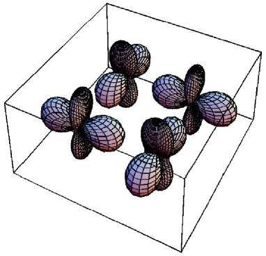
Figure 46: Alternating orbital order in FM cubic LaMnO₃ and in a 2D model of a FM $(a,b)$ plane in LaMnO₃: $(|x\rangle+|z\rangle)/\sqrt{2}$ an $(|x\rangle-|z\rangle)/\sqrt{2}$ as found at $E_{z}\to 0$ (after Ref. vdB99 ).

A finite orbital field $E_{z}\neq 0$ breaks the rotational symmetry on the classical level. It acts along the $c$-axis, and it is therefore easy to show that the ground state in the limit of $E_{z}\to 0$ is realized by the alternating occupied orbitals being symmetric/antisymmetric linear combinations of $|z\rangle$ and $|x\rangle$ orbitals, i.e., the occupied states correspond to the rotated orbitals (215) $|i\bar{\mu}\rangle$ and $|i\bar{\nu}\rangle$ on the two sublattices with an angle $\theta=\pi/4$, shown in Fig. 46. In particular, this state is different from the alternating directional orbitals, $3x^{2}-r^{2}$ and $3y^{2}-r^{2}$, which might have been naively expected. It follows in the limit of degenerate orbitals from the ’orbital-flop’ phase, in analogy to a spin-flop phase for the Heisenberg antiferromagnet at finite magnetic field. With increasing (decreasing) $E_{z}$ the orbitals tilt out of the state shown in Fig. 46, and approach $|x\rangle$ $(|z\rangle)$ orbitals, respectively, which may be interpreted as an increasing FM component of the orbital polarization in the pseudospin model.

To describe the tilting of pseudospins due to the crystal-field $\propto E_{z}$ we make two different transformations (215) at both sublattices, rotating the orbitals by an angle $\theta=\frac{\pi}{4}-\phi$ on sublattice $A$,

$$\left(\begin{array}[]{c}|i\mu\rangle\\ |i\nu\rangle\end{array}\right)\!=\!\left(\begin{array}[]{cc}\ \ \cos(\frac{\pi}{4}-\phi)&\sin(\frac{\pi}{4}-\phi)\\ -\sin(\frac{\pi}{4}-\phi)&\cos(\frac{\pi}{4}-\phi)\end{array}\right)\!\left(\begin{array}[]{c}|iz\rangle\\ |ix\rangle\end{array}\right),$$ (220)

and using a similar transformation to Eq. (220) with an angle $\theta=\frac{\pi}{4}+\phi$ on sublattice $B$, so that the relative angle between the occupied orbitals $|i\mu\rangle$ ($i\in A$) and $|j\nu\rangle$ ($j\in B$) is $\frac{\pi}{2}-2\phi$, and decreases with increasing $\phi$. The operators $T^{x}_{i}$ and $T^{z}_{i}$ may be now transformed as in Eqs. (216) using the actual rotations by $\theta=\frac{\pi}{4}\pm\phi$, as given in Eq. (220). As before, the orbitals $|i\mu\rangle$ and $|j\nu\rangle$ are occupied on two sublattices, $i\in A$ and $j\in B$, respectively, and the orbital order in the classical state is described by the transformed operators $\langle T^{z}_{i}\rangle=-1/2$ and $\langle T^{z}_{j}\rangle=+1/2$, respectively.

Using the new operators $T^{x}_{i}$ and $T^{z}_{i}$, the transformed Hamiltonian (212) takes the form,

$${\cal H}^{\phi}=H_{\parallel}^{\phi}+H_{\perp}^{\phi}+H_{\tau}^{\phi},$$ (221)

$$H_{\parallel}^{\phi} = \frac{1}{2}J\sum_{\langle ij\rangle\parallel}\left[(2\cos 4\phi-1)T^{x}_{i}T^{x}_{j}+(2\cos 4\phi+1)T^{z}_{i}T^{z}_{j}\right.$$ (222)

$$\hskip 31.2982pt+2\sin 4\phi(T^{x}_{i}T^{z}_{j}-T^{z}_{i}T^{x}_{j})\pm\!\sqrt{3}(T^{x}_{i}T^{z}_{j}+T^{z}_{i}T^{x}_{j})\left.\right],$$

$$H_{\perp}^{\phi}=J\sum_{\langle ij\rangle\perp}\left[\right.(\cos 4\phi+1)T^{x}_{i}T^{x}_{j}+(\cos 4\phi-1)T^{z}_{i}T^{z}_{j}-\sin 4\phi(T^{x}_{i}T^{z}_{j}-T^{z}_{i}T^{x}_{j})\left.\right],$$ (223)

$$H_{\tau}^{\phi}=E_{z}\sum_{i}(\lambda_{i}\sin 2\phi T^{z}_{i}-\cos 2\phi T^{x}_{i}),$$ (224)

where $\lambda_{i}=-1$ for $i\in A$ and $\lambda_{i}=1$ for $i\in B$. The energy of the classical ground state is given by,

$$E_{\rm 3D}^{\rm MF}=-\frac{3}{4}J\cos 4\phi+\frac{1}{2}E_{z}\sin 2\phi,$$ (225)

and is minimized by,

$$\sin 2\phi=-\frac{E_{z}}{6J}.$$ (226)

The above result (226) is valid for $|E_{z}|\leq 6J$; otherwise one of the initial orbitals (either $|x\rangle$ or $|z\rangle$) is occupied at each site, and the state is fully polarized ($\sin 2\phi=\pm 1$).

In contrast, in the 2D case the cubic symmetry is explicitly broken, and the classical state is of a spin-flop type (Fig. 46). It corresponds to alternatingly occupied orbitals on the two sublattices in the plane, with the orbitals given by $\theta=\pi/4$ in Eq. (215) at $E_{z}=0$. A finite value of $E_{z}$ tilts the orbitals out of the planar $|x\rangle$ orbitals by an angle $\phi$, and the Hamiltonian reduces to

$${\cal H}^{\phi}_{2D}=H_{\parallel}^{\phi}+H_{\tau}^{\phi},$$ (227)

as there is no bond in the $c$-direction. The classical energy is

$$E_{\rm 2D}^{\rm MF}=-\frac{1}{4}J(2\cos 4\phi+1)+\frac{1}{2}E_{z}\sin 2\phi.$$ (228)

Therefore, one finds the same energy of $-3J/4$ as in a 3D model at orbital degeneracy. This demonstrates a particular frustration of orbital superexchange interactions, where the orbital energy cannot be gained from the third direction once the orbitals have been optimized with respect to the other two. The bonds along the third direction only allow for restoring the rotational symmetry in the 3D model on the classical level by rotating the orthogonal orbitals in an arbitrary way. The energy (228) is minimized by,

$$\sin 2\phi=-\frac{E_{z}}{4J},$$ (229)

if $|E_{z}|\leq 4J$; otherwise $\sin 2\phi=\pm 1$. Interestingly, the value of the field at which the orbitals are fully polarized is reduced by one third from the value obtained in three dimensions (226). This shows that although the orbital exchange energy can be gained in a 3D model only on the bonds along two directions in the alternating (orbital-flop) phase either at or close to $E_{z}=0$, one has to counteract the superexchange on the bonds in all three directions when the field is applied.

The superexchange in the orbital subspace is AF and one may map the orbital terms in the Hamiltonian (221) onto a spin problem in order to treat the elementary excitations within the LSW theory. It is convenient to derive the excitations for the spin-flop phase induced by an orbital-field starting from the rotated Hamiltonian (221). Here we choose the Holstein-Primakoff transformation Faz99 ; Aue94 for localized pseudospin operators ($T=1/2$),

$$T_{i}^{+}=\bar{a}^{{\dagger}}_{i}(1-\bar{a}_{i}^{{\dagger}}\bar{a}_{i})^{1/2},\hskip 19.91684ptT_{i}^{-}=(1-\bar{a}_{i}^{{\dagger}}\bar{a}_{i})^{1/2}\bar{a}_{i},\hskip 19.91684ptT_{i}^{z}=\bar{a}^{{\dagger}}_{i}\bar{a}_{i}-\frac{1}{2},$$ (230)

for $i\in A$ sublattice and

$$T_{j}^{+}=(1-\bar{b}_{j}^{{\dagger}}\bar{b}_{j})^{1/2}\bar{b}_{j},\hskip 19.91684ptT_{j}^{-}=\bar{b}^{{\dagger}}_{j}(1-\bar{b}_{j}^{{\dagger}}\bar{b}_{j})^{1/2},\hskip 19.91684ptT_{j}^{z}=\frac{1}{2}-\bar{b}^{{\dagger}}_{j}\bar{b}_{j},$$ (231)

for $j\in B$ sublattice. In the harmonic approximation the terms $\sim T_{i}^{z}T_{j}^{x}$ do not contribute to the boson Hamiltonian as they give only odd numbers of boson operators. Therefore, the phase dependence in the terms $\propto\pm\sqrt{3}$ is lost in the LSW approximation.

After performing a Fourier transformation to $\{\bar{a}^{{\dagger}}_{\vec{k}},\bar{b}^{{\dagger}}_{\vec{k}}\}$ operators, the Hamiltonian may be further simplified by using the symmetry in ${\vec{k}}$-space and introducing new boson operators,

$$a_{\vec{k}}=\frac{1}{\sqrt{2}}(\bar{a}_{\vec{k}}-\bar{b}_{\vec{k}}),\hskip 28.45274ptb_{\vec{k}}=\frac{1}{\sqrt{2}}(\bar{a}_{\vec{k}}+\bar{b}_{\vec{k}}).$$ (232)

which leads to the effective orbital Hamiltonian of the form,

$$H_{\rm LSW} = J\sum_{\vec{k}}\left[A_{\vec{k}}a^{{\dagger}}_{\vec{k}}a_{\vec{k}}+\frac{1}{2}B_{\vec{k}}(a^{{\dagger}}_{\vec{k}}a^{{\dagger}}_{-{\vec{k}}}+a_{-{\vec{k}}}a_{\vec{k}})\right]$$ (233)

$$+J\sum_{\vec{k}}\left[A_{\vec{k}}b^{{\dagger}}_{\vec{k}}b_{\vec{k}}-\frac{1}{2}B_{\vec{k}}(b^{{\dagger}}_{\vec{k}}b^{{\dagger}}_{-{\vec{k}}}+b_{-{\vec{k}}}b_{\vec{k}})\right],$$

where the coefficients $A_{\vec{k}}$ and $B_{\vec{k}}$ depend on angle $\phi$,

$$A_{\vec{k}} = 3-B_{\vec{k}},$$ (234)

$$B_{\vec{k}} = \frac{1}{2}\left[(2\cos 4\phi-1)\gamma_{+}({\vec{k}})+(\cos 4\phi+1)\gamma_{z}({\vec{k}})\right],$$ (235)

and the ${\vec{k}}$-dependence is given by $\gamma_{+}({\vec{k}})$, and by $\gamma_{z}({\vec{k}})$, defined by Eqs. (106) and (108), respectively. After a Bogoliubov transformation,

$$a_{\vec{k}}=u_{\vec{k}}\alpha_{\vec{k}}+v_{\vec{k}}\alpha^{\dagger}_{-{\vec{k}}},\hskip 28.45274ptb_{\vec{k}}=u_{\vec{k}}\beta_{\vec{k}}+v_{\vec{k}}\beta^{\dagger}_{-{\vec{k}}},$$ (236)

with the coefficients

$$u_{\vec{k}}=\sqrt{\frac{A_{\vec{k}}}{2\zeta_{\vec{k}}}+\frac{1}{2}},\ \ \ v_{\vec{k}}=-{\rm sgn}(B_{\vec{k}})\sqrt{\frac{A_{\vec{k}}}{2\zeta_{\vec{k}}}-\frac{1}{2}},$$ (237)

where $\zeta_{\vec{k}}=\sqrt{A_{\vec{k}}^{2}-B_{\vec{k}}^{2}}$, the Hamiltonian (233) is diagonalized and takes the following form,

$$H_{\rm LSW}=\sum_{\vec{k}}\left[\omega^{-}_{\vec{k}}(\phi)\alpha^{{\dagger}}_{\vec{k}}\alpha_{\vec{k}}+\omega^{+}_{\vec{k}}(\phi)\beta^{{\dagger}}_{\vec{k}}\beta_{\vec{k}}\right].$$ (238)

The orbital-wave dispersion is given by

$$\omega_{\vec{k}}^{\pm}(\phi)=3J\left\{1\pm\frac{1}{3}\left[(2\cos 4\phi-1)\gamma_{+}({\vec{k}})+(\cos 4\phi+1)\gamma_{z}({\vec{k}})\right]\right\}^{1/2}.$$ (239)

The orbital excitation spectrum consists of two branches like, for instance, in an anisotropic Heisenberg model Faz99 .

Figure 47: Orbital-wave excitations as obtained for different values of the crystal-field splitting $E_{z}$ for a 3D (left) and 2D (right) orbital superexchange model (212). The result shown for a 3D system at $E_{z}=0$ was obtained for the orbitals rotated by $\theta=\pi/4$ in Eqs. (215), and corresponds to the $E_{z}\to 0$ limit of the orbital-flop phase (after Ref. vdB99 ).

The dependence on the field $E_{z}$ is implicitly contained in the above relations via the angle $\phi$, as determined by Eq. (226) and for the 3D model. The orbital-wave dispersion for a 2D system, can easily be obtained from Eq. (239) by setting $\gamma_{z}({\vec{k}})=0$ and selecting $\phi$ according to Eq. (229). First we discuss the excitation spectra given by Eq. (239) shown in Fig. 47 for different crystal-field splittings $E_{z}$ for the 3D system, along different high-symmetry directions of the $fcc$ BZ appropriate for the alternating orbital order. Most interestingly, a gapless orbital-wave excitation is found for the 3D system at orbital degeneracy. Obviously, this is due to the fact that the classical ground state energy is independent of the rotation angle $\theta$ at $E_{z}=0$. At first glance, however, one does not expect such a gapless mode, as the Hamiltonian (214) does not obey a continuous SU(2) symmetry. The cubic symmetry of the model, however, is restored if one includes the quantum fluctuations, as shown in Fig. 48. Note that the quantum corrections found in the 3D orbital model (214) are somewhat smaller than those for the 3D Heisenberg antiferromagnet. They do depend on the rotation angle $\theta$, as the orbital-wave dispersion does.

As a special case, the orbital-wave dispersion for a quasi-2D situation in a 3D case can easily be obtained from Eq. (239) by eliminating the term $\propto\gamma_{z}({\vec{k}})$ and assuming $\phi=\pi/4$,

$$\omega_{\vec{k}}^{\pm}(\phi=\pi/4)=3J\sqrt{1\pm\gamma_{+}(\vec{k})}.$$ (240)

In a 3D system it applies to the ground state given by alternating $|x\rangle$ and $|z\rangle$ orbitals on the two sublattices, and one finds the largest quantum corrections, as this dispersion has a line of nodes along the $\Gamma-Z$ direction, i.e., $\omega^{-}_{(0,0,q)}=0$ for $0<q<\pi$. In higher order spin-wave theory, however, it might very well be that a gap opens in the excitation spectrum. We expect, however, that this gap, if it arises, is small, with its size being self-consistently determined by quantum fluctuations.

For the 2D system the situation at orbital degeneracy is quite different (see Fig. 47). The lack of interactions along the $c$-axis breaks the symmetry of the model already at $E_{z}=0$, opens a gap in the excitation spectrum,

$$\omega_{\vec{k}}^{\pm}(\phi=0)=3J\sqrt{1\pm\frac{1}{3}\gamma_{+}(\vec{k})},$$ (241)

and suppresses quantum fluctuations. Thus, one encounters an interesting example of a more classical behavior in lower dimension. In fact, the 1D model (214) is classical as only Ising interactions are left and the modes are dispersionless (local mode at $\omega_{k}=2J$).

At increasing the orbital field $|E_{z}|$, the 2D and 3D system resemble each other, with a large gap in the excitation spectrum at $|E_{z}|=2J$ ($|E_{z}|=3J$) in the 2D (3D) system (Fig. 47). At larger $|E_{z}|$ the gap gradually closes when an orbital field which compensates the energy loss due to the orbital superexchange between identical (FM) orbitals is approached. At this value of the field ($E_{z}=4J$ and $E_{z}=6J$ in a 2D and 3D model, respectively), the full dispersion of the orbital waves is recovered, the spectrum is gapless (Fig. 47), and the quantum fluctuations reach a maximal value. We would like to emphasize that this behavior is qualitatively different from the Heisenberg antiferromagnet, both in two and three dimensions, where the anomalous terms $\propto T_{i}^{+}T_{j}^{+}$ and $\propto T_{i}^{-}T_{j}^{-}$ are absent which results in the conserved total spin $T^{z}=\sum_{i}T_{i}^{z}$, and quantum fluctuations vanish at the crossover from the spin-flop to FM phase.

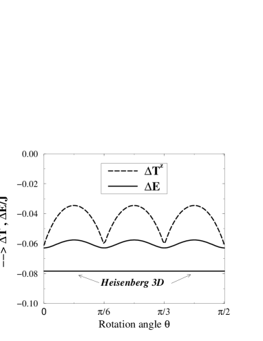
Figure 48: Quantum corrections for the 3D orbital model (212) as functions of rotation angle $\theta$ (215) for: the order parameter $\Delta T^{z}$ (full lines), and the ground-state energy $\Delta E/J$ (dashed lines) (after Ref. vdB99 ).

It is instructive to make a comparison between the analytic approximations of the LSW theory and the exact diagonalization (ED) of 2D finite clusters using the finite temperature diagonalization method Jak94 ; Jak00 . As in the mean-field approach, one finds also a unique ground state for finite clusters at $E_{z}=0$ by ED. Making the rotation of basis (215) is however still useful in the ED method as it gives more physical insight into the obtained correlation functions which become simpler and more transparent when calculated within an optimized basis. Moreover, they offer a simple tool to compare the results obtained by ED with those of the analytic approach. We shall present below the results obtained with $4\times 4$ clusters; similar results were also found for 10-site clusters Hor99 .

Let us look at nearest-neighbor correlation function in the ground state $\langle\tilde{T}^{z}_{i}\tilde{T}^{z}_{i+R}\rangle$, where the operators with a tilde refer to a rotated basis,

$$\tilde{T}^{z}_{i} = \cos 2\phi T^{z}_{i}+\sin 2\phi T^{x}_{i}$$

$$\tilde{T}^{z}_{i+R} = \cos 2\psi T^{z}_{i+R}+\sin 2\psi T^{x}_{i+R},$$ (242)

so that the correlation function depends on two angles: $\phi$ and $\psi$. In Fig. 49 the intersite orbital correlation in the ground state is shown as a contour-plot. The intensity of the grey scale changes from positive to negative values of the correlation function, $\langle\tilde{T}^{z}_{i}\tilde{T}^{z}_{i+R}\rangle$. One finds that the neighbor correlations have their largest value if the orbitals are rotated by $\phi=\pi/4$ and $\psi=3\pi/4$ (or $\phi=3\pi/4$ and $\psi=\pi/4$), i.e., under this rotation of the basis states the system looks like a ferromagnet, indicating that the occupied $(|x\rangle+|z\rangle)/\sqrt{2}$ and $(|x\rangle-|z\rangle)/\sqrt{2}$ orbitals are staggered in a 2D model, as shown in Fig. 46. Note that quantum fluctuations are small as in the ground state and one finds $\langle\tilde{T}^{z}_{i}\tilde{T}^{z}_{i+R}\rangle\simeq 0.246$. One finds that although the symmetry is not globally broken in a finite system, the short-range order resembles that found in the symmetry-broken state with orbital LRO. This demonstrates at the same time the advantage of the rotated basis in the ED study, because in the original unrotated basis one finds instead $\langle T^{z}_{i}T^{z}_{i+R}\rangle\simeq 0$, which might lead in a naive interpretation to a large overestimation of quantum fluctuations.

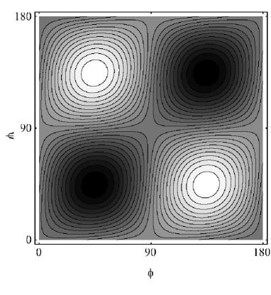
Figure 49: Contour plot of the rotated nearest-neighbor orbital correlation function $\langle{\tilde{T}}^{z}_{i}{\tilde{T}}^{z}_{i+R}\rangle$ as function of the angles $\phi$ and $\psi$ for a 16-site planar cluster with $E_{z}=0$ and $T=0.1J$. White regions correspond to positive (FM) and black areas to negative (AF) orbital correlations, i.e., $\langle{\tilde{T}}^{z}_{i}{\tilde{T}}^{z}_{i+R}\rangle>0.24$ ($<-0.24$), respectively. They are separated by 25 contour lines chosen with the step of 0.02 in the interval [-0.24,0.24] (after Ref. vdB99 .

Figure 50: Transverse response function ${\tilde{T}}^{+-}_{\bf q}(\omega)$ for the rotated orbitals as a function of frequency $\omega$ for different momenta at low temperature. Calculations were performed for a 16-site 2D cluster at $E_{z}=0$ and $T=0.1J$ for: (a) the 2D orbital model given by Eq. (214) ($H_{\rm full}$, full lines), and (b) neglecting the mixed terms $\propto T^{x}_{i}T^{z}_{j}$ ($H_{\rm trunc}$, dashed lines). The spectra are broadened by $\Gamma=0.1J$ (after Ref. vdB99 ).

The ground-state correlations $\langle\tilde{T}^{z}_{i}\tilde{T}^{z}_{i+R}\rangle$ found by ED are in excellent agreement with the results of LSW theory. By comparing the results obtained at $T=0.1J$, $0.2J$ and $0.5J$, it has been found in Ref. vdB99 that the calculated low-temperature correlation functions are almost identical in this temperature range, and thus the values shown in Fig. 49 for $T=0.1J$ are representative for the ground state. They demonstrate an instability of the system towards the symmetry-broken state.

In order to verify the accuracy of the LSW approach for finding the excitation spectrum, we discuss the results for the dynamical orbital response functions in the case of orbital degeneracy. The transverse response function for the orbital excitations evaluated with respect to the rotated local quantization axes (242) is defined as follows,

$${\tilde{T}}^{+-}_{\vec{q}}(\omega)=\frac{1}{2\pi}\int^{\infty}_{-\infty}dt\;\langle{\tilde{T}}^{+}_{\vec{q}}{\tilde{T}}^{-}_{-{\vec{q}}}(t)\rangle\;\exp(-i\omega t).$$ (243)

As we have already mentioned, the LSW approximation does not allow to investigate the consequences of the coupling of single excitonic excitations to the order parameter, represented by the terms $\propto T^{x}_{i}T^{z}_{j}$. Therefore, strictly speaking the LSW approach corresponds to the truncated Hamiltonian when such terms are not included. The ED gives then a double-peak structure in the response function ${\tilde{T}}^{+-}_{\vec{q}}(\omega)$ which agrees well with the dispersion of two modes found in the LSW approach (Fig. 50). However, if the terms $\propto T^{x}_{i}T^{z}_{j}$ are included, one finds different structures – the lowest energy excitation moves to lower energies, and satellite structures appear which describe the incoherent processes in orbital dynamics.

In spite of some additional incoherent processes in the spectra, the first moment of ${\tilde{T}}^{+-}_{\vec{q}}(\omega)$ determined by ED agrees very well with the dispersion found within the LSW theory [as determined from Eq. (241)] (Fig. 51). The values of the first moments are only slightly changed when instead the truncated Hamiltonian (without the processes $\propto T^{x}_{i}T^{z}_{j}$) is used in a numerical approach. This comparison demonstrates that the LSW approach captures the leading term in the orbital dynamics and may be thus used to investigate the consequences of orbital excitations on the hole dynamics, as presented in the next Section.

Figure 51: Dispersion of orbital waves along the main directions in the 2D BZ. Results for the first moment calculated for a $4\times 4$ cluster with the full ($H_{\rm full}$ and truncated ($H_{\rm trunc}$ Hamiltonian (empty and full symbols) are compared with the dispersions for the two modes found using the LSW theory (solid and dashed line) (after Ref. vdB99 ).

VII.2 Hole propagation in an orbital ordered state

As an interesting example of the consequence of orbital degrees of freedom in the hole excitation spectra, the problem of hole propagation in an orbital ordered 2D FM planes, as found in LaMnO₃, has been considered recently by van den Brink, Horsch and Oleś vdB00 . The main idea is that the hole which moves in an orbital ordered plane [Fig. 53(a)] dresses by orbital excitations, and a polaron is formed. Its properties will depend on the actual parameters and it is interesting to investigate: (i) whether a quasiparticle (QP) state will form under these circumstances in analogy with the spin problem – a hole moving in a quantum antiferromagnet Mar91 , and (ii) how much the spectral function changes when the orbital degeneracy is removed.

Let us consider the simplest situation and assume that the $e_{g}$ orbitals are degenerate, $E_{z}=0$. If only few holes are doped to a FM plane as in the A-AF phase of La_1-xCa_xMnO₃ with $x\ll 1$, the ground state is determined in first instance by a 2D version of the orbital model (214),

$$H_{J}=\frac{1}{2}J\sum_{\langle ij\rangle}\left[T^{z}_{i}T^{z}_{j}+3T^{x}_{i}T^{x}_{j}\mp\sqrt{3}(T^{x}_{i}T^{z}_{j}+T^{z}_{i}T^{x}_{j})\right],$$ (244)

where the bonds $\langle ij\rangle$ connect nearest neighbors in a single $(a,b)$ plane, and the AF superexchange $J$ implies that the orbitals order. In order to see the consequences of this ordered state for the kinetic energy of doped holes, it is convenient to transform the hopping term (38) along the bonds $\langle ij\rangle$ in the $(a,b)$ FM planes to the basis defined by Eqs. (220) at $\phi=0$ which corresponds to the symmetry-broken ground state with the orthogonal orbitals $|i\mu\rangle$ and $|j\nu\rangle$ occupied on the two sublattices (Fig. 46). Let us introduce the new fermion (hole) operators which correspond to the occupied orbitals $|i0\rangle$ as $f_{i0}^{\dagger}$, and the operators which correspond to the excited states $|i1\rangle$ as $f_{i1}^{\dagger}$. Thus, the operator $f_{i0}^{\dagger}$ create a hole in the orbital $|i\mu\rangle$ for $i\in A$ and $|i\nu\rangle$ for $i\in B$, respectively. The transformed kinetic energy is vdB00 ,

$$H_{t} = \frac{1}{4}t\!\sum_{\langle ij\rangle}\left[f_{i0}^{\dagger}f_{j0}+f_{i1}^{\dagger}f_{j1}+2(f_{i1}^{\dagger}f_{j0}+f_{i0}^{\dagger}f_{j1})\right.$$ (245)

$$\hskip 22.76228pt\left.\pm\sqrt{3}\left(f_{i1}^{\dagger}f_{j0}-f_{i0}^{\dagger}f_{j1}\right)+H.c.\right].$$

Together with the usual crystal-field splitting term $H_{\tau}$ (59), Eqs. (244) and (245) define the orbital $t$-$J$ model,

$${\cal H}=H_{t}+H_{J}+H_{\tau}.$$ (246)

The first interesting observation is that the hole motion is not completely suppressed by the orbital ordering, unlike in the spin $t$-$J$ model. The processes $\propto f_{i0}^{\dagger}f_{j0}$ concern the occupied orbitals and thus a hole may always interchange with an electron without disturbing the orbital ordering [Fig. 53(b)]. These processes lead to a band in the limit of $U\to\infty$, where the constraint of no double occupancy is implemented with the slave-boson operators $b_{i0}$ and $b_{i1}$, standing for the orbital flavors which accompany the hole operators $h_{i}^{\dagger}$ according to the prescription:

$$f_{i0}^{\dagger}=b_{i0}h_{i}^{\dagger},\hskip 28.45274ptf_{i1}^{\dagger}=b_{i1}h_{i}^{\dagger}.$$ (247)

In the orbital ordered state the $b_{i0}$ bosons are condensed, $b_{i0}=1$, which leads after a Fourier transformation from the hole operators $h_{i}^{\dagger}$ to $h_{\vec{k}}^{\dagger}$ to a free hole propagation in the lower Hubbard band,

$$H_{h}=\sum_{\vec{k}}\varepsilon^{0}_{\vec{k}}(\phi)h_{\vec{k}}^{\dagger}h_{\vec{k}},$$ (248)

with a dispersion determined by the orbital order via

$$\varepsilon^{0}_{\vec{k}}(\phi)=(-2\sin 2\phi+1)t\gamma_{+}({\vec{k}}),$$ (249)

where $\gamma_{+}({\vec{k}})$ is defined by Eq. (106). The angle $\phi$ (220) depends on the optimal orbitals (229): $\phi=0$ at the orbital degeneracy ($E_{z}=0$), while $\phi\neq 0$ if the orbital degeneracy is removed by a finite field $E_{z}\neq 0$. Note that the largest dispersion is found for $|x\rangle$ orbitals at $\phi=-\pi/4$, while the dispersion vanishes at $\phi=\pi/8$ due to the conflicting phases of $|x\rangle$ and $|z\rangle$ orbitals.

Figure 52: Dispersion relations in the reduced BZ [$X=(\pi,0)$, $S=(\pi/2,\pi/2)$] in the mean-field approximation which simulates the treatment of Coulomb repulsion in LDA+U as obtained for: $U=t$ (left), and in the lower Hubbard band centered at $\omega=0$ for $U=10t$ (right, full lines). In the right panel the dispersion obtained in the $U\rightarrow\infty$ limit is shown by dashed lines for comparison (after Ref. vdB00 ).

If the other processes which couple the moving hole to the orbital excitations could be neglected, the band (248) would give a coherent spectral function of a hole. Furthermore, an electron doped at $n=1$ would propagate in the upper Hubbard band by a similar dispersion, i.e., due to the term $\propto f_{i1}^{\dagger}f_{i1}$ in Eq. (245). These subbands are separated by the Coulomb interaction $U$ which acts between two $e_{g}$ states, in this case between the occupied and unoccupied orbital states,

$$H_{U}=U\sum_{i}f_{i0}^{\dagger}f_{i0}f_{i1}^{\dagger}f_{i1}.$$ (250)

We recall, however, that the interorbital Coulomb interaction is invariant with respect to the choice of orbital basis only if the pair-hopping terms in Eq. (39) are included Ole83 . In the present case with the occupied $|i0\rangle$ orbitals at $n=1$, we may take $f_{i0}^{\dagger}f_{i0}=1$, and the Coulomb term reduces to a local potential which acts on the unoccupied states $|i1\rangle$. When the hopping Hamiltonian (245) is supplemented by this potential $\propto U$, one finds that the bands are separated by a gap which opens at $U=0$ (Fig. 52). The bands change drastically as a function of $U$ vdB00 : if $U$ is small, the bands resemble the uncorrelated problem (178) of Sec. VI.A, while the shape of the lower Hubbard band becomes close to the $U\to\infty$ limit (248) already at $U/t\approx 10$ which may be taken a representative value for manganites Fei99 . These changes of the bands between the small and large $U$ regime simulate the effect of the local potentials which act on the unoccupied states in the LDA+U method Ani91 .

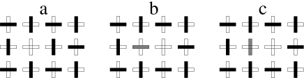
Figure 53: A single hole added in an orbital-ordered ground state (a); the occupied (empty) orbitals $|\mu\rangle$ and $|\nu\rangle$ are shown as filled (empty) rectangles. The hole can move either without disturbing the orbital order (b), or by creating orbital excitations (c) (after Ref. vdB00 ).

Thus, one finds a free hole band shown in Fig. 52 and the question is how this band changes when the hole starts to dress by orbital excitations of Sec.VII.A [Fig. 53(c)]. It may be expected that the free hole dispersion (248) is drastically modified by the hole-orbiton coupling which allows the hole propagation by frustrating the orbital order, just as the AF order is locally disturbed in the $t$-$J$ model, and the ’string’ of excited bonds is created on the path of the hole Shr88 . This problem was recently investigated in the orbital model by van den Brink, Horsch, and Oleś vdB00 who have shown that the interaction between the hole and the orbitals is so strong in the manganites that propagating holes are dressed with many orbital excitations and form polarons that have large mass, small bandwidth and low QP weight.

The orbital background is described by a local constraint for $T=1/2$ pseudospins,

$$b_{i0}^{\dagger}b_{i0}+b_{i1}^{\dagger}b_{i1}=2T,$$ (251)

where $b_{i0}^{\dagger}$ and $b_{i1}^{\dagger}$ are boson operators which refer to the occupied and empty state at site $i$ (247). By making the lowest order expansion of the constraint around the ground state with orbital ordering, one recovers the linear orbital-wave (LOW) approximation analyzed in Sec. VII.A. Having chosen the occupied orbitals as $b_{i0}^{\dagger}b_{i0}\simeq 1$ bosons at every site, the expansion is the same for both sublattices and reads,

$$T_{i}^{x}=\frac{1}{2}(b_{i}+b_{i}^{\dagger}),\hskip 28.45274ptT_{i}^{z}=T-b_{i}^{\dagger}b_{i},$$ (252)

with $b_{i}\equiv b_{i1}$ playing the role of a Holstein-Primakoff boson. It corresponds to the spin problem with the spins rotated by $\pi$ at one of the sublattices Faz99 ; Aue94 . The resulting effective boson Hamiltonian is diagonalized by a Fourier and Bogoliubov transformation (Sec. VII.A). One finds therefore an interacting problem in LOW approximation,

$${\cal H}_{\rm LOW}=H_{h}+H_{o}+H_{ho},$$ (253)

where the orbital waves (orbitons) for a 2D model are given by,

$$H_{o}=\sum_{\vec{k}}\omega_{\vec{k}}(\phi)\alpha^{{\dagger}}_{\vec{k}}\alpha_{\vec{k}},$$ (254)

with

$$\omega_{\vec{k}}(\phi)=3J\left[1+\frac{1}{3}(2\cos 4\phi-1)\gamma_{+}({\vec{k}})\right]^{1/2},$$ (255)

standing for the orbiton dispersion. The single mode written now for convenience in the full BZ in Eq. (254) is equivalent to two branches of orbital excitations obtained in the folded zone in Sec. VII.A vdB99 . The orbital excitations depend sensitively on the orbital splitting $E_{z}$. At orbital degeneracy ($E_{z}=0$) one finds a maximum of $\omega_{\vec{k}}(\phi)$ at the $\Gamma=(0,0)$ point and a weak dispersion $\sim J$ [see also Eq. (241)]. In contrast, for $E_{z}=\pm 2J$ orbital excitations are dispersionless, and $\omega_{\vec{k}}=3J$. The remaining part of Eq. (253) describes the hole-orbiton interaction [Fig. 53(c)],

$$H_{ho}=t\sum_{{\vec{k}},{\vec{q}}}h_{{\vec{k}}-{\vec{q}}}^{\dagger}h_{\vec{k}}\left[M_{{\vec{k}},{\vec{q}}}\alpha_{\vec{q}}^{\dagger}\right.+\left.N_{{\vec{k}},{\vec{q}}}\alpha_{{\vec{q}}+{\vec{Q}}}^{\dagger}+H.c.\right],$$ (256)

where ${\vec{Q}}=(\pi,\pi)$, the vertex functions are:

$$M_{{\vec{k}},{\vec{q}}} = 2\cos 2\phi\left[u_{\vec{q}}\gamma_{+}({\vec{k}}-{\vec{q}})+v_{\vec{q}}\gamma_{+}({\vec{k}})\right],$$ (257)

$$N_{{\vec{k}},{\vec{q}}} = -\sqrt{3}\left[u_{\vec{q}}\gamma_{-}({\vec{k}}-{\vec{q}})-v_{\vec{q}}\gamma_{-}({\vec{k}})\right],$$ (258)

and $\gamma_{-}({\vec{k}})=\gamma_{+}({k_{x},k_{y}+\pi})$ is defined by Eq. (107).

In this way, the orbital $t$-$J$ model (246) leads to an effective Hamiltonian (253), describing a many-body problem due to the hole-orbiton coupling term $H_{ho}$. Although the analytic structure and the form of Eq. (253) resembles the usual $t$-$J$ model written in the slave fermion formalism Mar91 , there are important differences. First of all, a hole may propagate freely in the orbital model by the term (249), as it would be also the case in the quantum antiferromagnet with further-neighbor hopping. Second, the orbital waves do not obey the nesting symmetry, i.e., $\omega_{{\vec{k}}+{\vec{Q}}}(\phi)\neq\omega_{\vec{k}}(\phi)$, where ${\vec{Q}}=(\pi,\pi)$, and are more classical than the spin waves, with a finite gap in the excitation spectrum (255). Furthermore, the hole-orbiton interaction (256) has a richer analytic structure than that of the $t$-$J$ model, as the scattering processes which conserve the momentum modulo ${\vec{Q}}$ due to a new vertex $\propto N_{{\vec{k}},{\vec{q}}}$ (258). Finally, an important feature is also that both hole dispersion $\varepsilon^{0}_{\vec{k}}(\phi)$ and orbiton dispersion $\omega_{\vec{k}}(\phi)$ depend on the crystal-field splitting $E_{z}$, and thus the analytic structure is richer. As a special case, at $E_{z}=-2J$ both modes are dispersionless, and the model orbital becomes equivalent to a hole which moves in a classical antiferromagnet described by the Ising model, with no quantum fluctuations Kan89 .

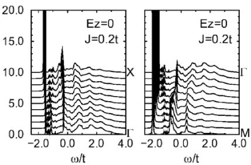
Figure 54: Spectral functions for the orbital $t$-$J$ model as obtained in two high-symmetry directions of the 2D BZ: $\Gamma-X$ (left) and $M-\Gamma$ (right) for $J=0.2t$ and $E_{z}=0$ [$\Gamma=(0,0)$, $X=(\pi,0)$, $M=(\pi,\pi)$] (after Ref. vdB00 ).

The many-body problem obtained for a hole propagating in an orbital ordered background (253) may be solved using the self-consistent Born approximation (SCBA) Sch89 ; Kane89 . This method gives results of high quality and compares favorably with ED for the hole which moves in a quantum antiferromagnet Mar91 . Treating ${\cal H}_{\rm LOW}$ in the SCBA, one finds the selfenergy vdB00 ,

$$\Sigma({\vec{k}},\omega) = t^{2}\sum_{\vec{q}}\left[M^{2}_{{\vec{k}},{\vec{k}}-{\vec{q}}}G({\vec{k}}-{\vec{q}},\omega-\omega_{\vec{q}})+N^{2}_{{\vec{k}},{\vec{k}}-{\vec{q}}}G({\vec{k}}-{\vec{q}},\omega-\omega_{{\vec{q}}+{\vec{Q}}})\right].$$ (259)

Here $G({\vec{k}},\omega)$ stands for the hole Green function which obeys the Dyson equation,

$$G^{-1}({\vec{k}},\omega)=\omega-\varepsilon^{0}_{\vec{k}}(\phi)-\Sigma({\vec{k}},\omega).$$ (260)

Eqs. (259) and (260) represent a closed set of equations which has to be solved numerically by iteration on a lattice. We discuss below some representative results obtained recently by van den Brink et al. vdB00 .

Figure 55: Ladder spectrum for the orbital $t$-$J$ model obtained for $E_{z}=-2J$ and $J=0.2t$ (after Ref. vdB00 ).

First of all, the hole spectral function is drastically changed by the coupling processes to the orbital excitations which is particularly strong when the orbital superexchange $J$ is much lower than the hopping $t$. Examples of rather complex spectra are shown in Figs. 54–56 for $J/t=0.1$ which corresponds to the realistic parameters for manganites Fei99 . As in the $t$-$J$ model, a QP state appears at the threshold, and this results from a strong dressing of a hole by a cloud of orbital excitations. The incoherent part extends over the scale of $\sim 6t$ which corresponds to the full dispersion in the $e_{g}$ band (178).

The energy and momentum dependence of the incoherent spectra is markedly different from the spin $t$-$J$ problem. At orbital degeneracy (Fig. 54) particular satellite structures are obtained with a rather weak ${\vec{k}}$-dependence. Their origin may be understood by looking at the hole spectrum found at $E_{z}=-2J$ which corresponds to the dispersionless orbiton spectrum (255) and to the vanishing hole dispersion (249) due to the conflicting phases in the $e_{g}$ electron hopping. In this case a ladder spectrum of the $t$-$J^{z}$ model is reproduced Kan89 ; Mar91 (Fig. 55), but the values of $t$ and $J^{z}$ have to scaled for the orbital model and the present case corresponds to a larger ratio $J^{z}/t\simeq 0.3$ in the spin problem vdB00 . Such ladder features at decreasing distances result in the pronounced satellites observed still in the spectra at orbital degeneracy. In contrast, with increasing value of $E_{z}$, the incoherent part changes to a rather smooth curve dominated by a broad maximum that corresponds to the free dispersion which is still visible but strongly damped by the hole scattering on the orbital excitations. An example of such spectra is shown in Fig. 56.

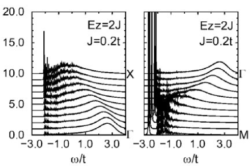
Figure 56: The same as in Fig. 54, but for $E_{z}=+2J$ (after Ref. vdB00 ).

The QP states have a narrow dispersion $\propto J$, as in the $t$-$J$ model (Fig. 57). Note that the QP’s are well defined and have a large weight $a_{M}$ close to the minimum of the QP band at the $M=(\pi,\pi)$ point, while they are weaker at higher energies. As in the $t$-$J$ model Mar91 , at the maximum of the QP band, found here at the $\Gamma=(0,0)$ point, the QP has the lowest spectral weight $a_{\Gamma}$. Note that the QP minimum is here determined by the minimum of free dispersion (Fig. 52) rather than by the enhanced quantum fluctuations at the boundary of the folded BZ, as encountered in the spin $t$-$J$ model.

The effective mass $m^{*}$ which may be defined be the momentum dependence of the QP energy vdB00 , and the QP bandwidth $W^{*}$ increase first linearly with increasing $J$ in the range of $J/t<0.3$, while they approach the free values in the weak-coupling regime of $J/t>1$. However, an additional dependence on the orbital splitting makes the QP dispersion rather narrow close to the orbital degeneracy ($E_{z}=0$) and at $E_{z}<0$, while it broadens up when $E_{z}>0$ and the uniform phase with $|x\rangle$ orbitals occupied is approached. This has interesting consequences for the experimental situation and suggests that the photoemission spectra of manganites should have a strong dependence on the deviations from the cubic symmetry which remove the orbital degeneracy $(E_{z}\neq 0$). Furthermore, the dependence on the doping might be very interesting in these situations when the orbital ordering changes, as for instance in the layered compounds Mac99 .

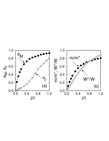
Figure 57: Quasiparticle properties at $E_{z}=0$ as functions of $J/t$: (a) weights of the two QP bands at the $\Gamma$ point: $a_{M}$ (filled circles), and $a_{\Gamma}$ (open squares); (b) inverse effective mass $m/m^{*}$ (full circles) and the width of QP band $W^{*}/W$ (empty circles), normalized by the LDA+U values $m$ and $W$, respectively (after Ref. vdB00 ).

VIII Phase diagrams of manganites – open problems

VIII.1 Magnetic, orbital, and charge ordering in CE-phase

Over the last few years much attention has been focused on the interplay between charge and orbital ordering occurring in half-doped manganites ($x=0.5$). A direct evidence of the charge ordered (CO) state in half-doped manganite has been provided by the electron diffraction for La_0.5Ca_0.5MnO₃ Cheo96 . Similar observations have also been reported for Pr_0.5Sr_0.5MnO₃ Tom95 Nd_0.5Sr_0.5MnO₃ Kuw95 , and for Pr_1-xCa_xMnO₃ with $x=0.4$ and 0.5 Zim99 . This CO state is characterized by an alternating arrangement of Mn³⁺ and Mn⁴⁺ ions in $(a,b)$ planes and the charge stacking in $c$-direction. In CO state these systems show an insulating behavior with a very peculiar form of AF spin ordering. The observed magnetic structure is the so-called magnetic CE phase and consists of quasi-1D FM zigzag chains coupled antiferromagnetically in both directions. In addition, the occupied orbitals at Mn³⁺ positions show in these systems $d_{3x^{2}-r^{2}}$/$d_{3y^{2}-r^{2}}$ orbital ordering, staggered along the FM chains.

The insulating CO state can be transformed into a metallic FM state either by doping, or by applying an external magnetic field Ima98 . Other interesting observations were done by studying Pr_1-x(Ca_1-ySr_y)_xMnO₃ crystals with controlled one-electron bandwidth. As already mentioned above, at half-doping Pr_0.5Ca_0.5MnO₃ has a CO CE-type insulating state. However, by substitution Ca with Sr leading to the increase of the carrier bandwidth, one induces the collapse of the CO insulating state, and the A-type metallic state with $d_{x^{2}-y^{2}}$ orbital ordering is realized in Pr_0.5Sr_0.5MnO₃ Kaw97 . The coexistence of the A-type spin ordered and CE-type spin/charge ordered states has been detected in the bilayer LaSr₂Mn₂O₇ Kub98 and in 3D Nd_0.5Sr_0.5MnO₃ Kuw95 . These results indicate the competition between the metallic A-type (uniform) $d_{x^{2}-y^{2}}$ orbital ordering, and the insulating CE-type $d_{3x^{2}-r^{2}}/d_{3y^{2}-r^{2}}$ orbital ordering at half-doping and demonstrate the importance of the coupling between magnetic, charge and orbital ordering in these compounds.

Figure 58: View of the CE phase in the $(a,b)$ plane. The $x^{2}-y^{2}$ orbitals at corner sites have positive (white) and negative (grey) lobes, while the phases of the other orbitals are positive. The grey dots at the bridge sites represent a charge surplus (after Ref. Kho99 ).

Being experimentally well established, theoretically, however, the nature of the CO state in half-doped manganites and the origin of the unconventional zigzag magnetic structure remain challenging open problems. As shown in Fig. 58, the CE-phase unit cell contains two geometrically inequivalent sites Kho99 , so-called bridge and corner sites. Note that the specific choice of basis orbitals shown in Fig. 58 is motivated by the convenience of this basis for the calculation of electronic structure. The expectation values of actual observables such as the charge distribution and the type of occupied orbitals are, of course, independent of the choice of basis Wannier orbitals.

It is straightforward to solve the band structure problem at no electron interactions Solce . The hopping elements follow from the Slater-Koster rules Zaa93 , and are shown in Fig. 59. The kinetic energy $H_{t}$ is given by the same expression as in Eq. (38), with the hopping integrals connecting now the orbitals along a single FM chain of the CE phase. We note that the unit cell consists of four atoms, but the electronic problem is simplified by a particular choice of orbital phases Kho99 . The orbitals perpendicular to the chain direction at the bridge positions $|\xi\rangle$ are decoupled from the directional $|\zeta\rangle$ orbitals and from $|x\rangle$ and $|z\rangle$ orbitals at corner sites – hence the bands are obtained by the solution of a $3\times 3$ matrix. One finds two bands with energies $\epsilon_{\pm}(k)=\pm t\sqrt{2-\cos 2k}$, where $k$ is the wave vector ($0<k\leq\pi/2$), and two nondispersive bands at zero energy. In Fig. 59 we reproduce the bands reported in Ref. Kho99 , where a different convention was used and the gap was found at $k=\pi/2$; the conventional definition of momentum $k$, however, leads with the alternating phases of $x^{2}-y^{2}$ orbitals at corner sites to the gap at $k=0$.

At $x=0.5$ the $\epsilon_{-}(k)$ band is fully occupied, and all other bands are empty. The system is insulating as the occupied and empty bands are separated by a gap $\Delta=t$ at $k=0$. In the C and CE phase the FM chains are decoupled due to the DE mechanism (Sec. II.B), and the kinetic energy is supplemented by the magnetic energy, equal for both structures. However, the opening of the gap at the Fermi-energy in the CE phase lowers its kinetic energy if the lowest band is filled, i.e., the system is half-doped. This mechanism is equivalent to the situation known from the lattice-Peierls problem, where the opening of a gap stabilizes the ground state with a lattice deformation. In the half-doped manganites, however, the gap is a direct consequence of the symmetry of the $e_{g}$ wave functions and is therefore a very robust feature.

Figure 59: Top: topology of the hopping in a zigzag chain, where $t_{1}=t/2$, $t_{2}=t\sqrt{3}/2$, and $U$ is the Coulomb interaction (261). Bottom left: electron dispersion in the zigzag chain of the CE phase for $U=0$, and electron dispersion in a C phase (dashed line). Bottom right: total energy per site for the CE, C and FM phase for $t/J=5$. The Maxwell construction in the phase separated (PS) region is shown by the thin dashed line (after Ref. Kho99 ).

In the insulating state at $x=0.5$ the average occupancy of the $|\zeta\rangle$ orbital at the bridge site ($3x^{2}-r^{2}$ or $3y^{2}-r^{2}$) is $n_{b}=\langle n_{m\zeta}\rangle=1/2$, while the orthogonal $|\xi\rangle$ orbitals at bridge positions are empty. The charge is thus uniformly distributed, with the average occupancy at the corner sites equal to $n_{c}=\langle n_{ix}+n_{iz}\rangle=1/2$, and the ratio between $|x\rangle$ and $|z\rangle$ occupancy of $n_{x}:n_{z}=\sqrt{3}:1$. This ratio reflects simply the ratio of hopping amplitudes between the bridge $|\zeta\rangle$ orbital and both orbitals at the corner positions. This symmetry in charge distribution is removed when the Coulomb interaction $U$ between $e_{g}$ electrons occupying different orbitals at the same site is taken into account. Using the above notation we write the Coulomb interaction as follows,

$$H_{U}=U\left(\sum_{m\in B}n_{m\zeta}n_{m\xi}+\sum_{i\in C}n_{ix}n_{iz}\right),$$ (261)

where $n_{i\alpha}=c^{\dagger}_{i\alpha}c_{i\alpha}$ are the respective electron number operators, and the summations run over bridge ($m\in B$) and corner ($i\in C$) positions of zigzag chains. For the $e_{g}$ electrons in the manganites $U\approx 10t$, so that the system is strongly correlated. We have verified using a HF approximation Cuo00 that the interactions have a very different effect on the corner and bridge-sites. On the bridge positions the $|\xi\rangle$ orbitals are always empty, so that the Coulomb repulsion is ineffective. In contrast, both orbitals ($|x\rangle$ and $|z\rangle$) are partially occupied on the corner sites, and thus the total electron density $n_{c}$ decreases with increasing $U$. The same effect was found by ED of finite clusters and with the Gutzwiller projection method by van den Brink, Khaliullin, and Khomskii Kho99 .

The phase diagram at different doping and $U=0$ in depicted in Fig. 59. We observe that CE-phase is stable only in the nearest vicinity of half-doping. For $x>1/2$ the holes that are doped into the lower $\epsilon_{-}$-band efficiently suppress the CO state. In this doping range the CE phase becomes unstable with respect to the C phase, and the kinetic energy of the C phase is lower for $x>0.57$ (Fig. 59). For $x<1/2$ the energy per site of the CE phase is constant because the extra electrons are doped in the nondispersive bands at zero energy; this is reflected by a kink obtained in the energy as a function of doping at $x=1/2$. For lower hole-doping (higher electron concentration) the homogeneous FM phase is more stable, as expected.

The interest in the origin of CO is also motivated by recent experimental data. The charge order functions are markedly stronger than the orbital fluctuations, both below and above the magnetic transition Zim99 . Thus it appears that the transition is driven by CO fluctuations, and the orbital state follows. Recognizing that the on-site Coulomb interaction between the orbitals at corner sites (261) leads to the CO state, we point out that another possibility to stabilize this state follows from the long-range Coulomb repulsion. Thus we consider the two-orbital FM Kondo lattice model (173) filled by $n=0.5$ electron per site,

$$H=-\sum_{ij\alpha\beta\sigma}t_{ij}^{\alpha\beta}c_{i\alpha\sigma}^{\dagger}c_{j\beta\sigma}-J_{H}\sum_{i\alpha\sigma\sigma{{}^{\prime}}}{\vec{S}}_{i}\cdot c_{i\alpha\sigma}^{\dagger}\vec{\sigma}_{\sigma\sigma{{}^{\prime}}}c_{i\alpha\sigma{{}^{\prime}}}+J_{AF}\sum_{\langle ij\rangle}{\vec{S}}_{i}\cdot{\vec{S}}_{j}+V\sum_{\langle ij\rangle}n_{i}n_{j},$$ (262)

which is extended by the intersite Coulomb repulsion $V$. On-site Coulomb interaction is not included, however, so the previous mechanism is absent. Studying the model (262) within the MF approximation, a competition between different types of magnetic ordering was established Jac00 . Let us compare the phase diagrams obtained for a nondegenerate Kondo lattice model (23) extended by a similar intersite Coulomb interaction term $\propto V$, and for the two-orbital model (262). In the case of the one-orbital model the MF theory predicts a ’continuous increase of the CO due to the intersite Coulomb interaction $V$. Depending on the value of the intersite Coulomb interaction $V$ and on superexchange coupling $J_{AF}$, different types of spin ordering shown in Fig. 60 (A-AF, C-AF, G-AF, and FM) coexist with the CO in the ground state of the one-orbital model. In contrast, in the two-orbital model the transition to the CO states occurs only at a finite critical value of $V$; thus magnetic states are obtained either with or without CO, depending on the value of $V$.

Figure 60: Phase diagram of the one-orbital model (left) two-orbital model (262) (right) for different values of $JS^{2}/t$ ($J=J_{AF}$) and $V/t$ parameters. Here A, C, and G stand for different magnetic ordering: A-AF, C-AF, G-AF and FM, respectively, and CO is charge ordering. The dashed line in the two-orbital case separates the uniform phase from the CO states in corresponding magnetic phases (after Ref. Jac00 ).

The presence of orbital degeneracy with the peculiar anisotropic hopping amplitudes between $e_{g}$ orbitals introduces a new magnetic state which was absent in the nondegenerate model, CE-type spin ordering (Fig. 60). In contrast to the nondegenerate case, the C-AF ordering is never found within the model (262) due to its instability against the effective ”dimerization” and the onset of the zigzag FM order. The alternation of the FM bonds in $a(b)$ directions leads to the alternation of the hopping amplitude. As a result the bare band is split into bonding and antibonding states and the ”dimerization” gap opens on the Fermi surface at half-doping. The CE-type spin ordered state is accompanied with $d_{3x^{2}-r^{2}}/d_{3y^{2}-r^{2}}$ orbital ordering that fits naturally to the topology of the zigzag structure as it was discussed above. The CE phase with magnetic and charge ordering as shown in Fig. 58 also wins over the charge disordered A-AF ordering in the regime of intermediate parameters. One may speculate that the competition between A-AF charge disordered and CE CO states indicates that parameters of the system are close to the critical values. Therefore, the small change of the bandwidth or the coupling to the lattice might stabilize one or the other state.

We have to conclude that these answers concerning the stability and the properties of the CE phase have to be treated as rather preliminary. The insulating behavior which follows from a topological phase factor in the hopping is certainly an interesting observation, and the CE phase seems to be indeed a particular type of order driven by the degeneracy of $e_{g}$ orbitals. The on-site and intersite Coulomb interactions are likely to help each other in stabilizing the CO states Mut99 . Although the intersite interaction stabilizes the CO state in a 2D lattice, it favors the same charge alternation in the third direction, contrary to the structure of the CE phase. This qualitative trend may by reversed only by other interactions. However, the precise role of different Coulomb interactions and of the JT effect in the stability of the CE phase Miz97 are not understood at present and have to be established by future studies.

VIII.2 Stripes in manganites

As we have discussed above, one of the unique aspects of physics of manganites is the unusually strong interaction between charge carriers and lattice degrees of freedom, due to which markedly distinct types of charge, orbital and magnetic ordering are observed in different doping regimes. The strong electron-phonon coupling, which can be tuned by varying the electronic doping, electronic bandwidth and disorder, gives rise to a complex phenomenology, in which crystallographic structure, magnetic structure and transport properties are intimately interrelated. Below a certain temperature $T_{CO}$, electronic carriers become localized onto specific sites, which display LRO throughout the crystal structure (CO states). Moreover, the filled $e_{g}$ ($3z^{2}-r^{2}$-like) orbitals at Mn³⁺ ions and the associated lattice distortions (elongated Mn–O bonds) also develop LRO (orbital ordering). Finally, the magnetic exchange interactions between neighboring Mn ions, mediated by oxygen ions, become strongly anisotropic which gives rise to complex magnetic ordering in the stable structures. Historically, magnetic ordering was the first to be experimentally investigated in manganites Wol55 , where the magnetic structures of a series of manganese perovskites with general formula La_1-xCa_xMnO₃ were studied using neutron powder diffraction. It was not until recently, however, that the crystallographic superstructure of this compound was experimentally observed by electron diffraction Rad97 . The curious static patterns in the spin, charge, and orbital densities observed in manganites are currently attracting much attention Che98 ; Che99 .

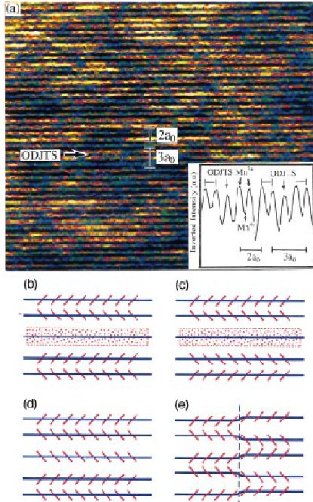
Figure 61: (a) High resolution lattice image in the FM phase at 206 K showing a mixture of incommensurate charge-ordered and FM charge disordered microdomains. The arrow stands for an unpaired JT stripes (JTS) between paired ones. An inverted intensity profile of this configuration is plotted in the inset of (a). (b) and (c) show in-phase and out-of-phase configurations, respectively, of the paired JTS surrounding the orbital disordered JTS. The lines represent Mn³⁺ JTS while the slanted slashes (random dotted strip) stand for $d_{z^{2}}$ orbital ordering (disordering). (b) and (c) go into residual discommensuration (d) and antiphase boundary (e), respectively, in the incommensurate phase when complete orbital order is realized (after Ref. Che98 ).

It is very interesting, that the charge and orbital ordering (COO) observed experimentally is always concomitant with the stripe-AF (S-AF) phase. At $x=1/2$, the COO, known as a CE phase (Sec. VII.B), has been confirmed by the synchrotron X-ray diffraction experiment Murce98 . At $x=2/3$, however, two different COO patterns have been reported: (i) the bistripe (BS) structure Che98 (Fig. 61), in which the main building block of the COO pattern at $x=1/2$ persists even at $x=2/3$, and (ii) the Wigner-crystal (WC) structure Rad99 , in which the COO occurs with the maximized distance between $e_{g}$ electrons. The appearance of these two different structures suggests that: (i) the corresponding energies are very close to each other and the ground state has (quasi-)degeneracy, and (ii) the conversion between them is prohibited by a large energy barrier. Under these circumstances, it is of limited relevance to investigate which of the two states has a lower energy using some model Hamiltonian. Rather than attempt to investigate which one gives the ground state for particular parameters, we present in extenso the recent ideas of Hotta et al. Hot00 on the origin of the near BS-WC degeneracy.

Let us discuss the importance of the role of the 1D conducting zigzag paths in the $(a,b)$ basal plane, and considered parallel-transport of an $e_{g}$ electron along these paths through the JT centers composed of MnO₆ octahedra. The transport invokes the Berry-phase connection and we can introduce the “winding number” $w$ as a direct consequence of topological invariance which should be conserved irrespective of the details of $H$. Consider $e_{g}$ electrons coupled both to localized $t_{2g}$ spins with the Hund’s rule coupling $J_{H}$, and to JT distortions of the MnO₆ octahedra. Since $J_{H}$ is the largest characteristic energy among those considered here, it is taken to be infinite for simplicity. This implies that the spin of each $e_{g}$ electron at a Mn site aligns completely in parallel with the direction of the $t_{2g}$ spin $S=3/2$ at the same site. Thus, the spin degrees of freedom are effectively lost for the $e_{g}$ electrons, and the spin index will be dropped hereafter. Since it is known experimentally that the $t_{2g}$ spins are antiparallel along the $c$-axis, we can assume that the $e_{g}$ electrons can move only in the $(a,b)$ plane due to the DE mechanism.

The above situation is well described by the Hamiltonian Hot00 ,

$$H = -\!\sum_{ij\alpha\beta}t^{\alpha\beta}_{ij}c_{i\alpha}^{{\dagger}}c_{j\beta}\!+\!J_{AF}\sum_{\langle ij\rangle}{\vec{S}}_{i}\cdot{\vec{S}}_{j}$$ (263)

$$+ \!E_{\rm JT}\!\sum_{i}\Bigl{[}2\sum_{\alpha\beta}c_{i\alpha}^{\dagger}(Q_{2i}\sigma_{i}^{x}+Q_{3i}\sigma_{i}^{z})_{\alpha\beta}c_{i\beta}+(Q_{2i}^{2}+Q_{3i}^{2})\Bigr{]},$$

with the same notation as used in Eq. (15). The second term $\propto J_{AF}$ represents the AF coupling between nearest-neighbor classical $t_{2g}$ spins which are normalized for convenience to $|{\vec{S}}_{i}|=1$. The third term is controlled by the JT energy $E_{\rm JT}$ and describes the coupling of an $e_{g}$ electron with the $(x^{2}$$-$$y^{2})$- and $(3z^{2}$$-$$r^{2})$-type (dimensionless) JT modes, given by $Q_{2i}$ and $Q_{3i}$ (Fig. 3), respectively.

Intuitively, it can be understood that the competition between kinetic and magnetic energies can produce an S-AF state. The ground state of the system described by Eq. (263) with $J_{AF}=0$ is a 2D FM metal and optimizes the kinetic energy of $e_{g}$ electrons, while it becomes a 2D AF insulator at $J_{AF}\geq t$ to exploit the magnetic energy of the $t_{2g}$ spins. For smaller but nonzero values of $J_{AF}$, a competition between these states occurs which results in a mixture of FM and AF states. In this S-AF state, a 1D conducting path can be defined by connecting nearest-neighbor sites with parallel $t_{2g}$ spins. A path with a large stabilization energy is needed to construct a stable 2D structure. Thus, Hotta et al. Hot00 concentrated themselves on specifying the shapes of (quasi-)stable 1D paths in the S-AF manifold.

Let us start with the case of $E_{\rm JT}$=$0$ and no electron correlation, which allows us to illustrate the importance of topology in the present problem. In a 2D FM metal, the kinetic-energy gain is reduced by $2J_{AF}$, due to the loss of magnetic energy per site. In contrast, in a 2D AF insulator, the magnetic energy gain per site is $2J_{AF}$. In S-AF states, the optimized periodicity $M$ for a 1D path along the $a$-axis direction is numerically found to be given by $M$=$2/n$ Hot00 , in agreement with Ref. Koi98 , where $n(=1-x)$ is the $e_{g}$-electron number per site. The S-AF structure with zigzag path is nothing but the well-known CE phase, and the analysis of Ref. Hot00 predicts that this state is very stable at $x$=1/2. However, the same analysis for $x\geq 2/3$ does not lead to a zigzag path but instead to a straight line as the optimized structure, which disagrees with experiment. Thus, it is necessary to find a quantity other than the energy to discuss the possible preferred paths that may arise from a full calculation, including nonzero $E_{\rm JT}$ and Coulomb interactions. Reconsidering the results at $x$=$1/2$ led Hotta et al. Hot00 to the idea that the number of vertices along the path, $N_{\rm v}$, may provide the key difference among paths. A confirmation of this idea is provided by the calculation of energies for the $2^{6}$ and $2^{8}$ paths at $x=2/3$ ($M$=6) and $3/4$ ($M$=8), respectively.

In the next step one may include the JT distortions, $E_{\rm JT}\neq 0$ in Eq. (263). By writing the JT modes in polar coordinates as $Q_{2i}=Q_{i}\sin\theta_{i}$ and $Q_{3i}=Q_{i}\cos\theta_{i}$, “phase-dressed” fermion operators, ${\tilde{c}}_{ix}$ and ${\tilde{c}}_{iz}$, are introduced as:

$${\tilde{c}}_{ix} = e^{i\theta_{i}/2}[c_{ix}\cos(\theta_{i}/2)+c_{iz}\sin(\theta_{i}/2)],$$ (264)

$${\tilde{c}}_{iz} = e^{i\theta_{i}/2}[-c_{ix}\sin(\theta_{i}/2)+c_{iz}\cos(\theta_{i}/2)],$$ (265)

with $e^{i\theta_{i}/2}$ representing the molecular Aharonov-Bohm effect. The amplitude $Q_{i}$ is determined by a MF approximation Hot00 , while the phases $\theta_{i}$’s are interrelated through the Berry-phase connection to provide the winding number $w$ along the 1D path as $w=\oint_{c}d{r}\cdot\nabla\theta/(2\pi)$, where $c$ forms a closed loop for the periodic lattice boundary conditions. Mathematically, the winding number $w$ is proven to be an integer Hot98 . In this system, it may be decomposed into two terms as $w=w_{\rm g}+w_{\rm t}$. The former, $w_{\rm g}$, is the geometric term which becomes $w_{\rm g}=0$ or 1, corresponding to the periodic or antiperiodic boundary condition in the $e_{g}$ electron wave function. It may be shown that the kinetic energy is lower with $w_{\rm g}$=$0$ than that with $w_{\rm g}$=$1$ for $x\geq 1/2$. Thus, $w_{\rm g}$ is taken as zero hereafter.

Figure 62: (a) A typical building block for a 1D path for an $e_{g}$ electron with JT distortions. (b) General structure of the lowest-energy-state path and the renormalization scheme for the vertices $\alpha$ and $\beta$. The thick (thin) line denotes the straight-line part with (without) an $e_{g}$ electron localized on it. The solid circle and diamond denote, respectively, the bare vertices, $\alpha$ and $\beta$, while open up-and down-triangles indicate the renormalized vertices, ${\tilde{\alpha}}$ and ${\tilde{\beta}}$. Note that the periodicity of the 1D path is given by $M=2/n=2/(1-x)$. (c) Groups of 1D paths derived from mother states with $m=0$ and 1. Paths in the first column corresponding to the mother WC structures with $w$=$2m$+$1$, which produce daughter states with $w=2m+2,2m+3,\cdots$ (after Ref. Hot00 ).

To show that only the number of vertices $N_{\rm v}$ along a given path determines the topological term $w_{\rm t}$, let us consider the transfer of a single $e_{g}$ electron along the path shown in Fig. 62(a). On the straight line part in either $a$- or $b$-direction, the phase is fixed at $\theta_{a}$=$2\pi/3$ ($\theta_{b}$=$4\pi/3$), because the $e_{g}$-electron orbital is polarized along the direction of the bridge bonds. This effect may be called an orbital double-exchange in the sense that the orbitals align along the actual chain direction to maximize the kinetic energy, similarly as the FM alignment of $t_{2g}$ spins in induced by the usual DE mechanism (Sec. II.B). Thus, $w_{\rm t}$ does not change when one of the bridge positions is passed. In contrast, when the electron passes by one of the vertex positions, the phase changes from $\theta_{a}$ to $\theta_{b}$ (from $\theta_{b}$ to $\theta_{a}$), indicating that the electron picks up a phase change of $2\pi/3$ ($4\pi/3$). Since these two vertices appear in pairs, $w_{\rm t}$(=$w$) is evaluated as $w_{\rm t}=(N_{\rm v}/2)(2\pi/3+4\pi/3)/(2\pi)=N_{\rm v}/2$. The phases at the corner positions are assigned as an average of the phases sandwiching those vertices, $\theta_{\alpha}=\pi$ and $\theta_{\beta}=0$, to keep $w_{\rm g}$ invariant. Then, the phases are determined at all the sites once $\theta_{x}$, $\theta_{y}$, $\theta_{\alpha}$, and $\theta_{\beta}$ are known.

Now we include the cooperative JT effect, important ingredient to determine COO patterns in the actual manganites. Although its microscopic treatment is involved, we can treat it phenomenologically as a constraint for macroscopic distortions Hot00 , energetically penalizing $w=0$ and $M/2$ paths. In fact, it is numerically found that $w=1,2,\cdots,M/2-1$ paths constitute the lowest-energy band and they can be regarded as degenerate, since its bandwidth is about $0.01t$, much smaller than the interband energy difference ($\sim 0.1t$). Summarizing, the cooperative JT effect gives us two rules for the localization of $e_{g}$ electrons Hot00 : (i) electrons never localize at vertices; (ii) electrons localize pairwise – any electron that localizes on one of the segments in the $a$-direction has a partner that localizes on one of the segments in the $b$-direction.

Applying these rules, we obtain a general structure for the lowest-energy path. Important features are the renormalized vertices, ${\tilde{\alpha}}$ and ${\tilde{\beta}}$, abbreviated notations to represent the set of straight-line parts that are not occupied by $e_{g}$ electrons. The winding number assigned to ${\tilde{\alpha}}$ (${\tilde{\beta}}$) is $1/3$+$w_{\alpha}$ ($2/3$+$w_{\beta}$), where the number of vertices included in ${\tilde{\alpha}}$ (${\tilde{\beta}}$) is $1$+$2w_{\alpha}$ ($1$+$2w_{\beta}$). Thus, the lowest-energy path is labeled by the nonnegative integers $w_{\alpha}$ and $w_{\beta}$, leading to a total winding number $w$=$1$+$w_{\alpha}$+$w_{\beta}$. Although the topological argument does not determine the precise position at which an $e_{g}$ electron localizes in space, it is enough to regard a charged straight-line part as a quasi-charge. Since the quasi-charges align at equal distance in the WC structure, the corresponding path is labeled by $w_{\alpha}$=$w_{\beta}=m$, with $m$ a nonnegative integer. By increasing $w_{\beta}$ keeping $w_{\alpha}$ fixed, we can produce any non-WC-structure paths with $w_{\alpha}=m$ and $w_{\beta}=m+1,m+2,\cdots$ [Fig. 62(c)]. In this way, the WC structure with $w=2m+1$ can be considered the mother state for all non-WC-structure paths with $w=2m+2,2m+3,\cdots$, referred to as the daughter states. The states belonging to different $m$’s are labeled by the same $w$, but a large energy barrier exists for the conversion among them, since an $e_{g}$ electron must be moved through a vertex in such a process. Thus, the state characterized by $w$ in the group with $m$, once formed, it cannot decay, even if it is not the lowest-energy state.

Note that the topological argument works irrespective of the details of the Hamiltonian $H$, since $w$ is a conserved quantity. However, it cannot single out the true ground state, since the quantitative discussion on the ground state energy depends on the choice of $H$ and on the approximations employed. In fact, either the BS or WC structure can be stable, but in view of the small energy difference, their relative energy will likely change whenever a new ingredient is added to $H$. It may be expected that these phases are rather sensitive to the Coulomb interactions which will play an important role in stabilizing one of these two structures.

Now we analyze following Hotta et al. Hot00 the charge and orbital arrangement in La_1-xCa_xMnO₃ ($x>0.5$), in which the experimental appearance of the BS structure provides key information to specify the 1D path. Since the quasi-charges exist in a contiguous way in the BS structure, its path is produced from the mother state with $m=0$ [see Fig. 62(c)]. In particular, the COO pattern in the shortest 1D path is uniquely determined as shown in Figs. 63. At $x=1/2$, the path is characterized by $w=1$ which is the basic mother state with $m=0$. The COO pattern shown in Fig. 63(a) leads to the CE-type AF state Murce98 . The other paths with $w=2$ and 3 are nothing but the BS structures experimentally observed at $x=2/3$ and 3/4 Che98 .

It may be assumed that the long-range Coulomb interaction $V$ destabilizes the BS structure and transforms it to the WC structure, but this is not the case; for the BS $\rightarrow$ WC conversion with the help of $V$, an $e_{g}$ electron must be on the vertex in the path with $w$=$2$ or $3$ [see Figs. 63(b) and 63(c)]. This is against rule (i) and thus, the BS structure, once formed, is stable due to the topological condition, even including a weak repulsion $V$. In the group of $m=0$, the WC structure appears only in the path with $w=1$. Thus, the WC-structure paths with $w=1$ at $x=2/3$ and 3/4 are obtained by simple extension of the straight-line part in the path at $x=1/2$ [see Figs. 63(d) and 63(e)]. The detailed charge distribution inside the quasi-charge segment is determined by a self-consistent calculation with the JT effect, leading to the WC structure. Even if the non-WC structure occurs for $w=1$, it is unstable in the sense that it is easily converted to the WC structure, because no energy barrier exists for an $e_{g}$ electron shift along the straight-line part.

Figure 63: (a) Path with $w=1$ at $x=1/2$ for $E_{\rm JT}=2t$. At each site, the orbital shape is shown with its size in proportion to the orbital density. (b) The BS-structure path with $w=2$ at $x=2/3$. (c) The BS-structure path with $w=3$ at $x=3/4$. (d) The WC-structure path with $w=1$ at $x=2/3$. (e) The WC-structure path with $w=1$ at $x=3/4$ (after Ref. Hot00 ).

The above topological analysis shows that: (i) the WC structure is made of $w_{\rm WC}$=$1$ zigzag paths, and (ii) the BS structure contains a shorter-period zigzag path with $w_{\rm BS}=M/2-1=x/(1-x)$. Note that on the BS path, the less-distorted Mn⁴⁺ sites occupy all the vertices ($N_{\rm v}$ equals the number of Mn⁴⁺ ions), while the heavily distorted Mn³⁺ sites appear in pairs (the number of Mn³⁺ ions equal to $2$). Thus, $w_{\rm BS}$ is rewritten as

$$w_{\rm BS}={N_{\rm v}\over 2}={{\rm Number~{}of~{}Mn}^{4+}~{}{\rm ions}\over{\rm Number~{}of~{}Mn}^{3+}~{}{\rm ions}}={x\over 1-x}.$$ (266)

Since $w_{\rm BS}$ is an integer, we can predict that at specific values of $x$[=$w_{\rm BS}$/($1$+$w_{\rm BS}$)], such as $1/2$, $2/3$, $3/4$, etcetera, nontrivial charge and orbital arrangement will be stabilized in agreement with the experimental observation Che98 .

VIII.3 Orbital ordering and phase separation

Finally, we turn to the competition between different magnetic phases in doped manganites. There is no controversy on the fact that ferromagnetism at large doping is promoted by the DE mechanism – the kinetic energy of $e_{g}$ electrons is maximized when the $t_{2g}$ spins and their own spins are aligned. Within this scenario, one gets a natural explanation of the FM metallic phase. When an $e_{g}$ electron moves in some region, it does not pay an energy $J_{H}$ if all the $t_{2g}$ spins in its neighborhood are parallel. The hole-spin scattering is reduced in this way, and one gains the kinetic energy. As the carrier concentration increases, the FM polarization clouds around the holes start to overlap and the ground state becomes metallic, with $e_{g}$ electrons moving in the correlated degenerate band, inducing the saturated FM ordering.

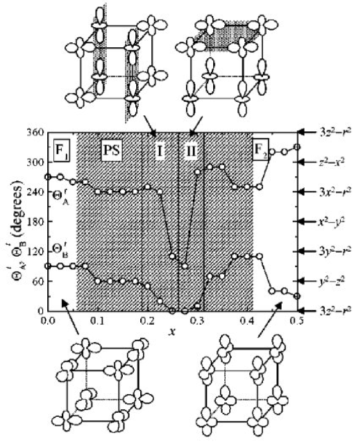
Figure 64: A sequential change of orbital states as a function of hole concentration $x$ (after Ref. Ish00 ). $\Theta_{A(B)}^{t}$ is the angle in the orbital space in the $A(B)$ orbital sublattice. Note that these angles are related to the angle used in Eq. (9) by $\theta_{A(B)}=2\Theta_{A(B)}^{t}$. The schematic orbital states are shown in phase-$I$ and phase-$II$; the dotted areas show the regions where the hole concentration is rich.

The understanding of the role played by the orbital degrees of freedom in the FM metallic phase is not complete, however. As suggested by the studies of DE both in the electron and hole doping regime Bri99 ; Ish00 ; Mae98 , one possibility is that the orbital ordering of some type is stabilized in particular doping regimes. The transitions between different types of orbital ordering are promoted by the kinetic energy which is optimized by either planar $|x\rangle$-type or directional $|z\rangle$-type orbitals, while the kinetic energy in the phases with orbital ordering and occupied orbitals that are linear combinations of $|x\rangle$ and $|z\rangle$ states as in Eqs. (III.2) is lower Kha00 ; Fei00 . This explains the mechanism of an orbital liquid discovered by Nagaosa et al. Nag97 , and confirmed by numerical studies Mac99 .

It has been found that due to a competition between the superexchange which favors orbital ordering and DE which favors a uniform phase, the magnetic phase diagrams obtained from the models which include the degeneracy of $e_{g}$ orbitals have orbital ordering also in the FM phase Ish00 ; Mae98 . An example is shown in Fig. 64, where all FM states have some kind of orbital ordering, modified under increasing doping. Such states are in qualitative agreement with the experimental observations at low doping, where the orbital ordering was observed in La_0.88Sr_0.12MnO₃ End99 , and may be concluded from the anisotropic exchange interactions found in La_0.85Ca_0.15MnO₃ Mou00 . The charge is uniformly distributed in this doping regime, while the orbital ordering occurs only in low temperatures in La_0.88Sr_0.12MnO₃, with a FM phase with disordered orbitals in the intermediate temperatures End99 . At higher doping, the transition to the orbital liquid state is indeed realized in double-layered manganites, where it is consistent with the observed lattice deformation along $c$ axis and allows to explain the observed the observed spin ordering and its anisotropy Nag00

In contrast, two phases (I and II) found for $0.18<x<0.32$ doping (Fig. 64) are characterized by the doped holes concentrated either in the regions of directional (I), or planar (II) orbitals, separated by the 1D or 2D structures with few holes and the orbitals being closer to the undoped situation. Whether or not such a competition between the phases with differently ordered orbitals really happens close to $x\sim 0.25$ is still controversial at the moment – it might be that the phase diagram of Okamoto, Ishihara, and Maekawa Ish00 is closer to the situation found in the insulating rather than metallic FM manganites. In fact, this competition suggests that there are also other ways of gaining the kinetic energy in the metallic phase, as for instance realized in uniform orbital phases with complex coefficients of $e_{g}$ orbitals Fei00 , and such states might be better candidates in the metallic phase.

Figure 65: Spectral functions $A({\vec{k}},\omega)$ at $J_{H}=\infty$ for a 2D one-orbital case with $T=1/30$, $\langle n\rangle\sim 0.92$, on a $12\times 12$ cluster for: (a) along $(\pi,0)$ to $(\pi,\pi)$; (b) along $(0,0)$ to $(\pi,\pi)$. Part (c) shows the results for the 2D two-orbital model with $T=1/10$, $\lambda=1.5$, $\langle n\rangle\sim 0.70$, on a $10\times 10$ cluster along $(0,0)$ to $(\pi,0)$ (after Ref. Mor99 ).

The experimental phase diagrams of manganites (Fig. 4) are typically richer than those obtained from model calculations. For instance, the phase diagram of Fig. 64 shows several different types of orbital ordering, but the magnetic state is FM in the whole range of doping $0<x<0.5$. Instead, the A-AF order is observed at small doping Mou99 , and CE-phase (Sec. VIII.A) at doping $x\simeq 0.5$. It is rather difficult to reproduce this complex behavior in the theoretical models. However, the interplay of charge, spin, lattice and orbital degrees of freedom belongs to the generic features of this class of compounds, and the challenge in the theory is still to describe these various energy contributions with comparable and sufficient accuracy.

The competition between the fully polarized FM state and other types of order which occurs as temperature and electron concentration are varied is a central problem in the physics of manganite perovskites. This problem has attracted a lot of interest recently, especially due to the unusual experimental results obtained in the manganese oxides Ram97 ; cheong . For instance, above the Curie temperature $T_{C}$ and for a wide range of densities, several manganites show an insulating behavior of not completely clear origin that contributes to the large magnetoresistance effects. The low temperature phases have complex structures, not fully understood within the DE scheme, that includes different phases with AF and CO ordering, orbital ordering, FM insulating phase, and tendencies towards the formation of charge inhomogeneities even in the FM phase. Moreover, many experimental results show the occurrence of charge inhomogeneities in macroscopic form or in small clusters of one phase embedded into another. It turns out the metallic FM phase has regions where FM clusters coexist with another phase in a range of temperature and concentration Sch95 ; Ram96 , either in Sr- and Ca-doped manganese oxides.

In this context, De Gennes suggested rather early that the competition between the AF superexchange and the DE results in the canting of the AF state deG60 , that is the angle $\theta$ between the spins from different sublattices becomes smaller than $\pi$. The canting angle grows with the concentration of charge carriers, which might explain the increase of magnetization upon doping observed in La_1-xCa_xMnO₃. Already rather long ago arguments were given against the stability of canted ground state Nag79 ; Nag96 . In the De Gennes approach the local spins were treated classically. It was found that quantum corrections stabilize the AF state and the canted state appears only above a certain concentration of charge carriers Nag96 . By this mechanism the canted state might also disappear – in fact it was not observed in La_1-xCa_xMnO₃ at increasing doping $0<x<0.15$ Mou99 .

A more fundamental problem however is that at partial filling of the conduction band, the homogeneous ground state might be unstable against phase separation (PS). Experimentally the PS was recently observed by Babushkina et al. Bab99 , and it is also obtained in theory. For instance, the phase diagram of Fig. 64 contains several regions with PS, either between different orbital states, or between differently doped phases. Another possibility is the PS between the regions with different magnetic ordering which accompanies differently doped regimes of the sample. This implies that many experimental data on doped manganites should be reinterpreted taking into account the inhomogeneity of the ground state. In particular, the charge transport and the metal-insulator transition should be more appropriately described in terms of percolation rather than by the properties of the pure states.

The problem of the nature of the PS has been studied extensively by means of QMC techniques within the FM Kondo model with one and two orbitals, including the JT effect for taking into account the occurrence of orbital order, though without fully considering the consequences of large Coulomb interactions Yun98 ; Hu98 . Several unexpected results have been found in that study. In particular, either for the one- or two-orbital model, when calculating the density of $e_{g}$ electrons as a function of varying chemical potential, one finds that some densities are unstable Yun98 ; Hu98 ; that is, the density is changing discontinuously at particular values of the chemical potential. Other calculations done in the canonical ensemble where the density is kept fixed, showed that the ground state is not homogeneous, while being constituted by separate regions with values of densities corresponding to the unstable regime. This phenomenon is usually referred to as phase separation, such as the familiar liquid-vapor coexistence in the phase diagram of water where it is known that the compressibility becomes negative negative. It is also similar to the stripe instability in the cuprates Zaa98 , but the present phenomenon is more difficult to study as it happens in a larger space which involves the orbitals and lattice.

In the regime of large Hund’s coupling $J_{H}$ and intermediate values of the JT coupling, PS occurs both for small and large hole densities. In particular at small $e_{g}$ densities, the PS appears between an electron-undoped AF state and a metallic uniform orbital-ordered FM state. At small hole concentrations, the latter phase coexists with an insulating staggered orbital ordered FM phase. In the QMC results Yun98 ; Hu98 , the PS manifests itself as the occurrence of a macroscopic separation of two phases with different charge distribution. Actually, this possibility should be prevented by long-range Coulomb interactions, which is usually neglected. In fact, even taking into account polarization effects and screening, a complete separation would lead to a huge loss of energy. These considerations suggest that two large regions should split into many smaller pieces in order to distribute the charge more uniformly and reduce the energy loss in the Coulomb channel.

If the PS involves just single carriers (doped holes) with their local environment that has been distorted by the presence of a hole, such states are referred to as polarons. The distortion can be either in the magnetic channel (spin polaron), or in the phononic channel (lattice polaron), or in the orbital channel (orbital polaron), or may be even a combination of these effects. Furthermore, the case where such regions of reduced electron density involve more than one carrier are referred to as clusters or droplets. The competition between the long-range Coulomb repulsion and the magnetic interaction would determine the size and the shape of the resulting clusters. The stable state, obtained when the extended Coulomb interactions are included, is considered as a charge inhomogeneous state which has to be distinguished from the metastable state that appears in a standard first order transition.

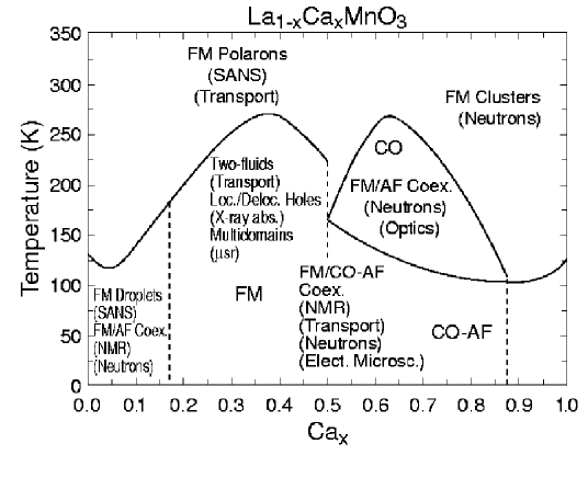
Figure 66: A schematic version of the phase diagram for La_1-xCa_xMnO₃ Sch95 . The abbreviations Coex., Loc., Deloc., abs., $\mu$SR, and Elect. Microsc., stand for coexistence, localized, delocalized, absorption, muon spin relaxation, and electron microscopy, respectively (after Ref. Adriana ).

A large-scale PS is expected if the competing phases have approximately the same density, as it happens experimentally at $x=0.5$ which is a singular point in the phase diagrams (Sec. VII.B). It is of fundamental importance to investigate how the properties of the ordered FM state are influenced by the vicinity of a PS regime, especially in connection to the CMR phenomenon. One of the consequences of this proximity to PS state is observed as an effective increase of the compressibility in the FM phase which implies the occurrence of strong charge fluctuations. This result implies that even within the FM phase, which is uniform when time averaged, there is a dynamical tendency toward cluster formation. This effect is expected to influence the transport property. Calculations done on finite size clusters show that the resistivity behaves as observed experimentally, in other words it is insulating at small $x$ and rapidly decreases when $x$ increases, and a metallic state is approached.

A very interesting observation was made recently by Moreo, Yunoki and Dagotto that the PS is responsible for a pseudogap formation in the spectral function $A({\vec{k}},\omega)$ calculated using Monte-Carlo techniques for the model of manganites which includes the coupling to JT phonons Mor99 . The pseudogaps was found to be a robust feature at all momenta along the Fermi surface and occurs due to the existence of FM clusters coexisting with the AF ordering. A particularly pronounced pseudogap was found in the model with doubly degenerate $e_{g}$ orbitals which demonstrates again that the orbital degrees of freedom play an important role in manganites. The results have striking similarity with the angle resolved photoemission studies of La_1.2Sr_1.8Mn₂O₇ Des98 which suggests that microscopic inhomogeneities exist in this system, both above and below $T_{C}$.

The PS scenario is likely to play an important role in the low and intermediate doping regime, where several mechanisms have been proposed to explain the CMR effects in manganese oxides. It adds to the simple DE idea the possibility of charge inhomogeneities as the main effect competing with ferromagnetism. This picture is different from that proposed by Millis et al. Mil95 , where the interplay between spin disorder and the formation of lattice polarons via JT-coupling is fundamental for explaining the metal-insulator transition. In this respect, though the JT-coupling turns out to be important in both scenarios, in the PS scheme a state given by independent local lattice polarons is a special case of a more general situation where droplets of various shape and size might form. Still, the dynamical fluctuation of charge inhomogeneities increase as T_C decreases, thus explaining the CMR effect at the boundary of the FM phase. Other theories emphasize the electronic localization effect induced by off-diagonal disorder in the spin correlations Mul96 ; Var96 ; Cal98 , or diagonal disorder due to chemical substitution.

Summarizing, the generic phase diagram of manganites shown in Fig. 66 represents still a very challenging and interesting problem in the field of correlated electrons in degenerate $e_{g}$ bands. There are many open questions related to the understanding of the insulating state of manganese oxides, especially in the framework of tendencies towards charge inhomogeneous state. Analytical techniques beyond the local MF approximations are required to reproduce the essential physics of the nonuniform charge phase and to investigate the role of orbital ordering in doped manganites. More detailed analysis is needed to understand the shape and the size of droplets in such inhomogeneous states, and the crossover from the PS regime to polaronic regime which has been observed experimentally Uru95 ; cheong ; Fuj98 .

IX Summary and conclusions

We have reported a systematic analysis of the consequences of orbital degrees of freedom in a class of correlated MHI: copper and manganese oxides. These systems are characterized by several different interactions which involve three different types of degrees of freedom in the undoped compounds: spins, orbitals, and lattice. If such systems are doped, one has to include in addition charge dynamics. The main question we have been dealing with through this report was: What is the role of the orbital degrees of freedom in presence of strong electron correlations and/or lattice effects, and what kind of magnetic and orbital ordering is promoted by them?

The essence of the problem posed by the superexchange interactions at orbital degeneracy is captured by the spin-orbital model (57)–(59) for the cuprates, defined for the $d^{9}$ ions as in KCuF₃. This model is of particular interest as it combines only two aspects of a more complex problem: magnetic (spin) and orbital degrees of freedom, which are discussed at integral filling, i.e., in the absence of doping, and without taking seriously into account the JT effect. The model Hamiltonian has already been proposed long ago Kug73 , but its full consequences have been appreciated only recently Fei97 ; Ole00 .

The Hamiltonian derived for the cuprates from the spectroscopic information about the spectra of excited states has been first considered on the classical level, where we have shown in Sec. III that it gives a particular frustration of spin and orbital interactions. This is best represented by a singular point at the origin of the phase diagram for the $d^{9}$ spin-orbital model (Fig. 12) which is highly degenerate at the classical level, so that many axes separating different classical phases should emerge from it. In this respect the classical phase diagram is incomplete: the quantum mechanics is likely to take over in this regime and decide about the actual ordered or disordered state. As a main result of this part, we have shown that enhanced quantum fluctuations close to the transition lines between different classical phases destroy classical states (Sec. IV). Unlike in the frustrated spin models, the Gaussian fluctuations around classical states involve the orbital sector, probably yielding novel spin-orbital liquids in the form of generalized (R)VB states Fei97 . Such states turn out to be very good variational wave functions, and turn out to be exceptionally stable in the $d^{9}$ model with respect to the classical phases.

Whether the phase diagram presented in Fig. 31 is the qualitatively correct picture of the quantum disorder realized next to the orbital degeneracy, is still an open question. Another possibility would be an ordered state which results by the order-out-of disorder mechanism. Unfortunately, even the physics at the above multicritical point of the phase diagram of the $d^{9}$ model is not captured by the SU(4) model which, instead, turns out to be an idealized generalization of the Kugel-Khomskii model, putting the spin and orbital variables on the same footing. However, this highly symmetric problem is not easier to investigate except for the 1D case, and thus the final answer to the problem of the ground state of the spin-orbital $d^{9}$ model in the vicinity of the multicritical point is still an open issue.

The physical properties of a system described by the spin-orbital model (57)–(59) are mainly determined by the nature of the collective excitations. In addition to the usual magnon dispersion known from the spin systems, we have to consider the pure orbital (or excitonic) excitations, and the mixed modes which involve simultaneously both spin and orbital excitation (spin-and-orbital modes). These modes couple to the magnons and may thus have measurable consequences, predicted as an anomalous spin response detected in neutron scattering experiments. It is thus challenging for the experimentalists to investigate carefully any peculiarities which are expected to arise in the spin spectra of the MHI with orbital degeneracy.

The above ideas on the spin liquid near orbital degeneracy and on the role played by the orbital fluctuations should be verified by future experiments. It is not easy to find compounds whose microscopic parameters live in the region close to this peculiar point in the phase diagram, and a progress in material science in needed. Furthermore, though close to this region in the sector of the electronic interactions, the cooperative and local JT effects convey to remove the orbital degeneracy stabilizing a particular spin pattern, as for example, it is realized in NaNiO₂. In this respect, an interesting situation seems to happen in the case of LiNiO₂, where these competing lattice-induced phenomena that promote ordered states are absent, and a quantum critical state characterized by power-law behavior of the spin correlation functions appears instead.

The spin-orbital model (159) derived for the $d^{4}$ ions as in LaMnO₃ Fei99 has many common features with the simpler model in the $d^{9}$ case (Sec. V). The spin interactions are different as they concern large spins $S=2$ of Mn³⁺ ions, and more excited states of Mn²⁺ ions are involved, even when the $e_{g}$ part of superexchange (157) is considered alone. As a consequence of larger spins, the model is more classical and the disordered states are not likely taking the realistic situation in manganites, with the strong JT effect which drives the system away from the multicritical point of frustrated interactions. The classical phases in the $d^{4}$ case are similar to those found for the $d^{9}$ model, but quantitatively the regions of their stability are different. Therefore, the A-AF phase obtained by a particular interrelation between the magnetic and orbital ordering is obtained in the $d^{4}$ case in a natural way as a consequence of the $e_{g}$ part of superexchange interactions – this phase is robust and agrees with experimentally observed ordering in manganites. An important finding in this respect is that the electronic mechanism alone is responsible of the A-AF ordering, and that the JT interaction is only changing this state quantitatively and tuning a somewhat different orbital ordering. Furthermore, when a FM $(a,b)$ plane of the A-AF phase is considered, the spins are integrated out and one finds the same orbital part of the superexchange Hamiltonian discussed in Sec. VII.

The analysis of the $d^{9}$ and $d^{4}$ models may be treated as the first step on the way towards the understanding of one of the most challenging problems in the modern solid state physics: How the delicate balance of magnetic and orbital interactions is affected by doping in the manganese oxides, and which physical mechanisms are responsible for various types of ordering observed in the CMR materials? We have analyzed this issue in an extensive way in Secs. V-VIII. Firstly, we have discussed the low doping regime of the manganese oxides which is simpler because the lattice helps to restrict the doped holes to particular sites, and the model deals in principle still only with the same degrees of freedom as in undoped LaMnO₃: spin, orbital, and lattice, but they are modified by the added charges. This part of the phase diagram is dominated by many competing effects both in the magnetic and orbital channel. The central issue is the presence of an orbital polaron regime which mediates the crossover from the A-AF to the FM insulating phase. The DE mechanism stabilizes the polarons and their localization by new FM effective interactions that give rise to the transition to the FM insulating phase as the hole concentration is increased (Sec. V.B). The binding energy of these orbital-hole bound state depends on the scale of fluctuations that involve orbitals, and therefore on the concentration of doped holes. Different configurations of the polarons may be stabilized by the lattice effects; the polarons are separated from each other Ahn98 and may induce interesting orbital ordering in their neighborhood Miz00 , but finally start to overlap. Thus, when the hole concentration increases, the orbital fluctuations also do, breaking eventually the localization process and favoring instead a different kind of orbital (ordered or disordered) state in a FM metallic phase. This problem is at heart of the CMR phenomenon.

Naively, the transition to the FM metallic phase occurs due to the DE mechanism. This picture is oversimplified – it ignores the orbital degrees of freedom which are of importance in the doped regime and lead to several types of magnetic ordering when the DE model is generalized to the case of degenerate $e_{g}$ orbitals (Sec. VI). We would like to emphasize that the DE via degenerate orbitals has very interesting special features that are very different from the conventional nondegenerate situation. The orbital degeneracy leads in general to the formation of anisotropic magnetic structures that depend on the actual doping concentration, and include the layered magnetic A-type structures, predominantly the $x^{2}-y^{2}$ orbitals, and chain-like structures of the C-type. The stability of such states will be influenced by lattice distortions – in this case a compression of the MnO₆ octahedra along one of the cubic directions. One can show, however, that due to the anharmonicity the JT distortion always leads to a local elongation. If strong enough along the $c$-axis, this tendency would favor a structure in which the $3z^{2}-r^{2}$ orbitals are occupied, in this case lowering the energy of C-type structures. These considerations demonstrate the importance of the JT effect. Cooperative JT coupling between the individual MnO₆ centers in the crystal leads to the simultaneous ordering of the octahedral distortions and the electronic orbitals. Part of the electronic energy is thereby lost and therefore an accurate description of the orbital state in manganites is possible only when the lattice effects are explicitly included in the model.

Unlike the DE Hamiltonian for nondegenerate orbitals, the realistic DE model which includes the degeneracy of $e_{g}$ electrons cannot be considered without the strong Coulomb correlations. Electronic correlations are very important for the understanding CMR manganites and cannot be neglected. Very different results are obtained when local Coulomb correlations are not included – for instance: the tendency towards the FM metallic phase is strongest at the filling of one $e_{g}$ electron per site Sol99 , and the band gap practically vanishes without JT distortions Pop00 , while in reality the gap is primarily due to large on-site Coulomb interactions Var96 (Sec. VII). The main result of the DE model without Coulomb interactions is that it can explain FM metallic phase only for doping $x>0.5$, where, however, the localized G-AF phases are typically found (Fig. 4). At lower values of $x$, the suppression of double occupations by the local Coulomb repulsion becomes more and more important, and leads to a crossover from DE to superexchange. First it reduces somewhat the effective FM interactions which follow from the DE mechanism, leading to the reduction of the magnon bandwidth pm99 and of the Curie temperature $T_{C}$ Hel00 with decreasing $x$, and eventually the superexchange between the Mn³⁺ ions becomes more important and stabilizes the A-AF ordering coexisting with the orbital ordering.

Recently it became clear that the nature of FM states may be studied by analyzing the spectrum of magnetic excitations. In recent neutron scattering experiments Per96 ; End97 ; Hwa98 the spin wave dispersion throughout the BZ was measured in various manganites in the FM phase. It has been found that the spin waves are clearly resolved at low temperature, and the stiffness constant shows a universal behavior. This universal behavior and also the higher-energy magnons in the metallic phase are well described by the DE model with degenerate $e_{g}$ orbitals, supplemented by smaller SE terms (Sec. VI.B). At higher temperature, however, different charge dynamics in metallic and localized compounds manifest themselves in the heavy damping of high-frequency spin waves even below T_c. Therefore, the simple DE model does not describe well the observed spectra in such situations when the doped holes localize, high-frequency magnons soften, and the value of $T_{C}$ is reduced. We have discussed that orbital and charge fluctuations are responsible for a strong modulation of the exchange bonds, leading to a softening of the magnon excitation spectrum close to the BZ boundary (Sec. VI.C). The presence of JT phonons further enhances this effect. This peculiar interplay between DE physics and orbital-lattice dynamics becomes dominant close to the instability towards an orbital-lattice ordered state. The unusual magnon dispersion experimentally observed in low-$T_{C}$ FM manganites can hence be considered as a precursor effect of orbital-lattice ordering. A complete understanding of these complex phenomena is still an open problem MN00 and may be achieved only by taking into account all relevant degrees of freedom, including the JT effect which is still present in the metallic phase Despi .

The proper understanding of pure orbital excitations is also very important, both in the undoped regime, and for the FM phase where such excitations are responsible for the orbital dynamics. Starting from the uniform FM phase, where the spin operators can be integrated out, we considered the interaction which occurs only between the pairs of ions with singly occupied staggered $e_{g}$ orbitals at nearest neighbor sites (Sec. VII). A gapless orbital-wave excitation is found for the 3D system at orbital degeneracy, a peculiarity related to the invariance of the classical ground state energy with respect to the orbital rotations by angle $\theta$ at $E_{z}=0$. This rotational invariance is broken in the 2D systems by the lack of interactions along the $c$-axis, and the 2D orbital model is more classical, with a gap in the excitation spectrum and suppressed quantum fluctuations, unlike in spin systems which are more quantum when one comes to a lower dimension. At increasing orbital field $E_{z}$, however, the system resembles again the behavior of a 3D system, with finite quantum fluctuations even when the orbitals are aligned which follows from the nonconservation of the orbital quantum number in the subspace of $e_{g}$ orbitals.

Another open problem is the mechanism of stability of the CE phase in half-doped manganites with $x=0.5$. The insulating CO state has been observed in almost all such compounds at half-doping, accompanied by a peculiar magnetic structure: 1D FM zigzag chains coupled antiferromagnetically within the $(a,b)$ planes, and along the $c$-axis. In addition, these systems show $d_{3x^{2}-r^{2}}$/$d_{3y^{2}-r^{2}}$ orbital ordering along the FM chains. The is no doubt that the degeneracy of $e_{g}$ orbitals plays here once again a crucial role. It follows both from a different behavior of the effective DE models with nondegenerate and degenerate orbitals, and from the specific mechanism of an insulating behavior discussed in Sec. VIII.A. The stability of different magnetic states is changed by orbital degeneracy, and for instance the C-type spin ordering is never achieved in the two-orbital case due to its instability against the effective dimerization and formation of the zigzag FM order. The alternating $d_{3x^{2}-r^{2}}/d_{3y^{2}-r^{2}}$ orbital ordering along the FM zigzag chain follows naturally the topology of the hopping in the CE phase. However, the role of the JT effect played in this phase and the magnetic and orbital excitation spectra are not yet understood.

The competition between different phases represents a particularly challenging problem. It results in a PS between AF and FM domains which together with the tendency to form inhomogeneous structures, seems to be a generic property of systems with strongly correlated electrons. Depending on the specific situation tuned by the strength of the coupling to the lattice and the doping level, the instability of homogeneous state and the tendency to PS may result in a formation of different structures: either random, percolation-like networks or regular structures, e.g. stripes, Wigner crystals, and the like (Sec. VIII). Many properties of such phase-separated states differ markedly from those of homogeneous states, and the possibility of PS has to serve as a starting point for the future explanation of certain anomalous phenomena observed experimentally in manganites. The PS scenario should lead to certain extensions of the DE model for degenerate $e_{g}$ orbitals by the ideas of charge inhomogeneities as the main effect competing with ferromagnetism, and by considering the insulating properties above the Curie temperature as a consequence of the formation of dynamical clusters. How the PS scenario occurs is still an open problem and it is related to the understanding of the insulating states in manganites and other materials with strongly correlated electron bands. Analytical techniques beyond the local MF approximations are required to get the essential physics of the non-uniform CO phase under control. In experiment, the photoemission spectroscopy is expected to be of particular importance, as such features as the pseudogap Mor99 , and the changes of the spectra between the compounds with different number of adjacent magnetic layers, lattice distortions, and doping levels, would help to characterize the orbital and magnetic ordering in the underlying phases.

Summarizing, the realistic model for manganites has to include the superexchange of spin-orbital type, the coupling to the lattice due to the cooperative and local JT effect, and some form of the DE in the correlated $e_{g}$ orbitals, either localized or itinerant. Several theoretical models have already been proposed, but in most cases they neglect at least one of the important aspects of the problem (as, for instance, either $e_{g}$ orbital degeneracy, or coupling to the lattice, or electron correlations), and then use some parameters to fit such properties as the type of magnetic ordering, the stiffness constant, or the types of occupied orbitals to the experiment — this is usually successful as the parameter space is large enough. While the model proposed by Feiner and Oleś Fei99 can certainly still be improved, it not only includes all the essential aspects mentioned above, but also takes the parameters from spectroscopy, except for the orbital interaction which follows from the JT effect and was fixed by experiment. In this way, the parameters which determine the magnetic transitions are all fixed and the predictions of this model may by confronted with experiment. The quality of this model may be appreciated by looking at Table 3. The Néel temperatures of the Mott-Hubbard insulators: LaMnO₃ and CaMnO₃, of the weakly doped polaronic La_0.92Ca_0.08MnO₃ compound, as well as the Curie temperature of the metallic FM La_0.7Pb_0.3MnO₃, are all obtained within 30 % to the experimental value. Of course, there is still a lot of room for improvement and the understanding is far from complete, in particular at finite temperature. Future progress may be expected by including the JT effect in a better way, and by a more careful analysis of the orbital ordered and disordered phases in various doping regimes.

We believe that the present report makes the role played by the correlated $e_{g}$ orbitals in the MHI more transparent, and demonstrates that they have to be included to obtain qualitatively correct answers in still open problems, such as: the stability of different phases including the CE phase and stripe phases, the mechanism of PS, the metal-insulator transition at finite temperature, and the mechanism of the CMR itself.

Table 3: Magnetic transition temperatures for the A-AF and G-AF states in undoped compounds: LaMnO₃, CaMnO₃, and in polaronic A-AF phase in La_0.92Ca_0.08MnO₃ ($T_{N}$), and in the metallic FM La_0.7Pb_0.3MnO₃ ($T_{C}$), as obtained from the spin-orbital model in doped manganites presented in Refs. Fei99 ; pm99 , including a reduction factor due to quantum fluctuations (theory), compared with the experimental values (exp). The physical mechanisms which contribute to the stability of these different magnetic phases are indicated by ’+’; DE effect was included either by polaronic (P) or by itinerant (I) mechanism. Orbital ordering stabilized by a superposition of the $e_{g}$-superexchange and the JT effect above $T_{N}$ plays a crucial role in driving the magnetic ordering in LaMnO₃ and in La_0.92Ca_0.08MnO₃ into the A-AF phase.

		superexchange				$T_{N}$ ($T_{C}$)
compound	phase	$e_{g}$ part	$t_{2g}$ part	DE	JT	theory	exp	Ref.
LaMnO3	A-AF	+	+	–	+	106 K	139 K	Mou99
La0.92Ca0.08MnO3	A-AF	+	+	P	+	95 K	122 K	Mou99
La0.7Pb0.3MnO3	FM	+	+	I	–	390 K	355 K	Hwa98
CaMnO3	G-AF	–	+	–	–	124 K	110 K	Wol55

- (1) M. Imada, A. Fujimori, and Y. Tokura, Rev. Mod. Phys. 70, 1039 (1998).
- (2) P. Fulde, Electron Correlation in Molecules and Solids, Springer, Berlin, 1995.
- (3) P. Fazekas, Lecture Notes on Electron Correlations and Magnetism, World Scientific, Singapore, 1999.
- (4) K. A. Chao, J. Spałek, and A. M. Oleś, J. Phys. C 10, L271 (1977).
- (5) K. A. Chao, J. Spałek, and A. M. Oleś, Phys. Rev. B 18, 3453 (1978).
- (6) J. Zaanen, G. A. Sawatzky, and J. W. Allen, Phys. Rev. Lett. 55, 418 (1999).
- (7) J. Zaanen and G. A. Sawatzky, J. Sol. State Chem. 88, 8 (1990).
- (8) M. Meinders, H. Eskes, and G. A. Sawatzky, Phys. Rev. B 48, 3916 (1993).
- (9) F. C. Zhang and T. M. Rice, Phys. Rev. B 37, 3759 (1988).
- (10) L. F. Feiner, J. H. Jefferson, and R. Raimondi, Phys. Rev. B 53, 8751 (1996).
- (11) J. H. Jefferson, H. Eskes, and L. F. Feiner, Phys. Rev. B 45, 7959 (1992).
- (12) R. Raimondi, L. F. Feiner, and J. H. Jefferson, Phys. Rev. B 53, 8774 (1996).
- (13) J. Zaanen and A. M. Oleś, Phys. Rev. B 37, 9423 (1988).
- (14) G. A. Gehring and K. A. Gehring, Rep. Prog. Phys. 38, 1 (1975).
- (15) K. I. Kugel and D. I. Khomskii, Usp. Fiz. Nauk (Sov. Phys. JETP) 136 (25), 621 (1982).
- (16) J. Zaanen and A. M. Oleś, Phys. Rev. B 48, 7197 (1993).
- (17) D. I. Khomskii and G. A. Sawatzky, Sol. State Commun. 102, 87 (1997).
- (18) K. I. Kugel and D. I. Khomskii, Zh. Eksp. Teor. Fiz. (Sov. Phys. JETP) 64 (37), 1429 (1973).
- (19) J. L. García-Munoz, J. Rodriguez-Carvajal, and P. Lacorre, Europhys. Lett. 20, 241 (1992).
- (20) M. L. Medarde, J. Phys.: Condens. Matter 9, 1679 (1997).
- (21) J. Rodriguez-Carvajal, S. Rosenkranz, M. Medarde, P. Lacorre, M. T. Fernandez-D az, F. Fauth, and V. Trounov, Phys. Rev. B 57, 456 (1998).
- (22) A. P. Ramirez, J. Phys. Cond. Matter. 9, 8171 (1997).
- (23) L. F. Feiner and A. M. Oleś, Phys. Rev. B 59, 3295 (1999).
- (24) C. Castellani, C. R. Natoli, and J. Ranninger, Phys. Rev. B 18, 4945 and 4967, and 5001 (1978).
- (25) W. Bao, C. Broholm, G. Aeppli, P. Dai, J. M. Honig, and P. Metcalf, Phys. Rev. Lett. 78, 507 (1997).
- (26) W. Bao, C. Broholm, G. Aeppli, S. A. Carter, P. Dai, T. F. Rosenbaum, J. M. Honig, P. Metcalf, , and S. F. Trevino, Phys. Rev. B 58, 12 727 (1998).
- (27) H. F. Pen, J. van den Brink, D. I. Khomskii, and G. A. Sawatzky, Phys. Rev. Lett. 78, 1323 (1998).
- (28) S. Y. Ezhov, V. I. Anisimov, D. I. Khomskii, and G. A. Sawatzky, Phys. Rev. Lett. 83, 4136 (1999).
- (29) A. I. J. W. L. M. v. Z. J. P. H. D. G. Y. T. B. Keimer, D. Casa and Y. Tokura, Phys. Rev. Lett. 85, 3946 (2000).
- (30) A. E. Bocquet, T. Mizokawa, K. Morikawa, A. Fujimori, S. M. Barman, K. B. Maiti, D. D. Sarma, Y. Tokura, and M. Onoda, Phys. Rev. B 53, 1161 (1996).
- (31) J. S. Griffith, The Theory of Transition Metal Ions, Cambridge University Press, Cambridge, 1971.
- (32) A. M. Oleś, Phys. Rev. B 28, 327 (1983).
- (33) A. M. Oleś and G. Stollhoff, Phys. Rev. B 29, 314 (1984).
- (34) G. Stollhoff, A. M. Oleś, and V. Heine, Phys. Rev. B 41, 7028 (1990).
- (35) V. I. Anisimov, J. Zaanen, and O. K. Andersen, Phys. Rev. B 44, 943 (1991).
- (36) A. I. Liechtenstein, V. I. Anisimov, and J. Zaanen, Phys. Rev. B 52 (1995).
- (37) V. I. Anisimov, I. S. Elfimov, M. A. Korotin, and K. Terakura, Phys. Rev. B 55, 15 494 (1997).
- (38) I. V. Solovyev, N. Hamada, and K. Terakura, Phys. Rev. Lett. 76, 4825 (1996).
- (39) K. Hirota, N. Kaneko, A. Nishizawa, and Y. Endoh, J. Phys. Soc. Jpn. 65, 3736 (1996).
- (40) F. Moussa, H. Henion, J. Rodriguez-Carvajal, H. Moudden, L. Pinsard, and A. Revcolevschi, Phys. Rev. B 54, 15 149 (1996).
- (41) J. Kanamori, J. Appl. Phys. 31, 14S (1960).
- (42) A. J. Millis, Phys. Rev. B 53, 8434 (1996).
- (43) H. Röder, J. Zhang, and A. R. Bishop, Phys. Rev. Lett. 76, 1356 (1996).
- (44) R. von Helmolt, J. Wecker, B. Holzapfel, L. Schultz, and K. Samwer, Phys. Rev. Lett. 71, 2331 (1993).
- (45) C. Zener, Phys. Rev. 82, 403 (1951).
- (46) P. W. Anderson and H. Hasegawa, Phys. Rev. 100, 675 (1955).
- (47) T. Hotta, S. Yunoki, M. Mayr, and E. Dagotto, Phys. Rev. B 60, R15 009 (1999).
- (48) J. C. Slater and G. F. Koster, Phys. Rev. 94, 1498 (1954).
- (49) P. A. Allen and V. Perebeinos, Phys. Rev. B 60, 10 747 (1999).
- (50) S. Yunoki, A. Moreo, and E. Dagotto, Phys. Rev. Lett. 81, 5612 (1998).
- (51) J. C. Slater, Phys. Rev. 49, 537 (1936).
- (52) P. W. Anderson, Phys. Rev. 115, 2 (1959).
- (53) J. Nagaoka, Phys. Rev. 147, 392 (1966).
- (54) J. H. Van Vleck, Rev. Mod. Phys. 25, 220 (1953).
- (55) M. Cyrot and C. Lyon-Caen, J. Phys. (Paris) 36, 253 (1975).
- (56) S. Inagaki, J. Phys. Soc. Jpn. 39, 596 (1975).
- (57) K. A. Chao, J. Spałek, and A. M. Oleś, Phys. Stat. Solidi (b) 84, 747 (1977).
- (58) J. Spałek and K. A. Chao, J. Phys. C 13, 5241 (1980).
- (59) A. J. Millis, P. B. Littlewood, and B. I. Shraiman, Phys. Rev. Lett. 74, 5144 (1995).
- (60) A. Urushibara, Y. Moritomo, T. Arima, A. Asamitsu, G. Kido, and Y. Tokura, Phys. Rev. B 51, 14 103 (1995).
- (61) Y. Okimoto, T. Katsufuji, T. Ishikawa, T. Arima, and Y. Tokura, Phys. Rev. B 55, 4206 (1997).
- (62) Y. Okimoto, T. Katsufuji, T. Ishikawa, A. Urushibara, T. Arima, and Y. Tokura, Phys. Rev. Lett. 75, 109 (1995).
- (63) L. F. Feiner, A. M. Oleś, and J. Zaanen, Phys. Rev. Lett. 78, 2799 (1997).
- (64) A. M. Oleś, L. F. Feiner, and J. Zaanen, Phys. Rev. B 61, 6257 (2000).
- (65) J. van den Brink and D. I. Khomskii, Phys. Rev. Lett. 82, 1016 (1999).
- (66) J. R. Schrieffer and P. A. Wolff, Phys. Rev. 149, 491 (1966).
- (67) G. Baym, Lectures on Quantum Mechanics, Benjiamin, NY, 1974.
- (68) E. Dagotto, Rev. Mod. Phys. 66, 763 (1994).
- (69) A. Georges, G. Kotliar, W. Krauth, and M. J. Rozenberg, Rev. Mod. Phys. 68, 13 (1996).
- (70) N. Furukawa, in Physics of Manganites , edited by T. A. Kaplan and S. D. Mahanti, Kluwer/Plenum, New York, 1999.
- (71) N. Furukawa, J. Phys. Soc. Jpn. 65, 1174 (1996).
- (72) K. Kubo and N. Ohata, J. Phys. Soc. Jpn. 33, 21 (1972).
- (73) J. B. Grant and A. K. McMahan, Phys. Rev. B 46, 8440 (1992).
- (74) A. I. Liechtenstein and D. I. Khomskii, Sov. Phys. JETP 52, 501 (1980).
- (75) D. H. Tennant, T. G. Perring, R. A. Cowley, and S. E. Nagler, Phys. Rev. Lett. 70, 4003 (1993).
- (76) H. Tennant, R. A. Cowley, S. E. Nagler, and A. M. Tsvelik, Phys. Rev. B 52, 13 368 (1995).
- (77) D. H. Tennant, S. E. Nagler, D. Welz, G. Shirane, and K. Yamada, Phys. Rev. B 52, 13 381 (1995).
- (78) L. F. Feiner, A. M. Oleś, and J. Zaanen, J. Phys.: Condens. Matter 10, L555 (1998).
- (79) J. van den Brink, W. Stekelenburg, D. I. Khomskii, G. A. Sawatzky, and K. I. Kugel, Phys. Rev. B 58, 10 276 (1998).
- (80) B. Sutherland, Phys. Rev. B 12, 3795 (1975).
- (81) B. Frischmuth, F. Mila, and M. Troyer, Phys. Rev. Lett. 82, 835 (1999).
- (82) A. Auerbach, Interacting Electrons and Quantum Magnetism, Springer, New York, 1994.
- (83) M. Takahashi, Phys. Rev. B 40, 2494 (1989).
- (84) D. N. Zubarev, Sov. Usp. Phys. 3, 320 (1960).
- (85) S. B. Haley and P. Erdös, Phys. Rev. B 5, 1106 (1972).
- (86) G. Khaliullin and V. Oudovenko, Phys. Rev. B 56, R14 243 (1997).
- (87) Y. Yamashita, N. Shibata, and K. Ueda, Phys. Rev. B 58, 9114 (1998).
- (88) Y. Q. Li, M. Ma, D. N. Shi, and F. C. Zhang, Phys. Rev. Lett. 81, 3527 (1998).
- (89) Y. Q. Li, M. Ma, D. N. Shi, and F. C. Zhang, Phys. Rev. B 60, 12 781 (1999).
- (90) P. Azaria, A. O. Gogolin, P. Lecheminant, and A. A. Nersesyan, Phys. Rev. B 83, 624 (1999).
- (91) A. Joshi, M. Ma, F. Mila, D. N. Shi, and F. C. Zhang, Phys. Rev. B 60, 6584 (1999).
- (92) F. Mila, B. Frischmuth, A. Deppeler, and M. Troyer, Phys. Rev. Lett. 82, 3697 (1999).
- (93) I. Affleck, Nucl. Phys. B265, 409 (1986).
- (94) G. Santoro, S. Sorella, L. Guidoni, A. Parola, and E. Tosatti, Phys. Rev. Lett. 83, 3065 (1999).
- (95) H. Bethe, Z. Phys. B 71, 205 (1930).
- (96) H. Evertz, G. Lana, and M. Marcu, Phys. Rev. Lett. 70, 875 (1993).
- (97) B. Beard and U. Wiese, Phys. Rev. Lett. 77, 5130 (1996).
- (98) M. van den Bossche, F. C. Zhang, and F. Mila, cond-mat/0001051.
- (99) S. K. Pati, R. Singh, and D. I. Khomskii, Phys. Rev. Lett. 81, 5406 (1998).
- (100) S. K. Pati and R. Singh, Phys. Rev. B 61, 5868 (2000).
- (101) P. Chandra and B. Doucot, Phys. Rev. B 38, 9335 (1988).
- (102) A. Moreo, E. Dagotto, T. Jolicoeur, and J. Riera, Phys. Rev. B 42, 6283 (1990).
- (103) N. Read and S. Sachdev, Phys. Rev. Lett. 66, 1773 (1991).
- (104) A. V. Dotsenko and O. P. Sushkov, Phys. Rev. B 50, 13 821 (1994).
- (105) N. B. Ivanov, S. E. Krüger, and J. Richter, Phys. Rev. B 53, 2633 (1996).
- (106) A. Chubukov, Phys. Rev. B 44, 392 (1991).
- (107) A. J. Millis and H. Monien, Phys. Rev. B 50, 16606 (1994).
- (108) A. W. Sandvik and D. J. Scalapino, Phys. Rev. Lett. 72, 2777 (1994).
- (109) A. V. Chubukov and D. K. Morr, Phys. Rev. B 52, 3521 (1995).
- (110) P. Anderson, Science 235, 1196 (1987).
- (111) C. K. Majumdar and D. K. Ghosh, J. Math. Phys. 10, 1388 (1969).
- (112) I. Affleck, T. Kennedy, E. Lieb, and H.Tasaki, Phys. Rev. Lett. 59, 799 (1987).
- (113) S. Sachdev, Quantum Phase Transition, Cambridge University Press, Cambridge, 1999.
- (114) J. Igarashi, J. Phys. Soc. Jpn. 62, 4449 (1993).
- (115) H. Schulz, T. Ziman, and D. Poilblanc, Magnetic systems with competing interactions, World Scientific, Singapore, 1994.
- (116) H. Schulz, T. Ziman, and D. Poilblanc, J. Phys. I (Paris) 6, 675 (1996).
- (117) S. Sachdev and R. Bhatt, Phys. Rev. B 41, 9323 (1990).
- (118) M. Gelfand, R. Singh, and D. Huse, Phys. Rev. B 40, 10 801 (1989).
- (119) V. Kotov, O. Sushkov, and R. Eder, Phys. Rev. B 59, 6266 (1999).
- (120) E. Lieb, T. Schultz, and D. Mattis, Ann. Phys. (N.Y.) 16, 407 (1961).
- (121) I. Affleck, Phys. Rev. B 37, 5186 (1988).
- (122) S. Sachdev and M. Vojta, cond-mat/9908008.
- (123) N. Katoh and M. Imada, J. Phys. Soc. Jpn. 62, 3728 (1993).
- (124) K. Ueda, H. Kontani, M. Sigrist, and P. A. Lee, Phys. Rev. Lett. 76, 1932 (1996).
- (125) O. A. Starykh, M. E. Zhitomirsky, D. I. Khomskii, R. Singh, and K. Ueda, Phys. Rev. Lett. 77, 2558 (1996).
- (126) M. Troyer, H. Kontani, and K. Ueda, Phys. Rev. Lett. 76, 3822 (1996).
- (127) S. R. White, Phys. Rev. Lett. 77, 3633 (1996).
- (128) E. Fradkin, Field theories of condensed matter systems, Addison-Wesley, NY, 1991.
- (129) F. Haldane, Phys. Rev. Lett. 61, 1029 (1988).
- (130) A. Sandvik, A. Chubukov, and S. Sachdev, Phys. Rev. B 51, 16483 (1995).
- (131) S. R. White, R. M. Noack, and D. J. Scalapino, Phys. Rev. Lett. 73, 886 (1994).
- (132) E. Dagotto and T. M. Rice, Science 271, 618 (1996).
- (133) M. Troyer, H. Tsunetsugu, and T. M. Rice, Phys. Rev. B 53, 251 (1996).
- (134) B. Normand and T. M. Rice, Phys. Rev. B 54, 7180 (1996).
- (135) K. Hirakawa, H. Kadowaki, and K. Ubokoshi, J. Phys. Soc. Jpn. 54, 3526 (1985).
- (136) K. Yamaura, M. Takano, A. Hirano, and R. Kanno, J. Solid State Chem. 127, 109 (1997).
- (137) Y. Y. Hsieh and M. Blume, Phys. Rev. B 6, 2684 (1972).
- (138) T. Mizokawa and A. Fujimori, Phys. Rev. B 54, 5368 (1996).
- (139) D. L. Cox, Phys. Rev. Lett. 59, 1240 (1987).
- (140) J. Zaanen, L. F. Feiner, and A. M. Oleś, Mat. Sci. Eng. B 69, 140 (1999).
- (141) S. A. Kivelson, D. S. Rokshar, and J. P. Sethna, Phys. Rev. B 35, 8865 (1987).
- (142) L. F. Feiner, A. M. Oleś, and J. Zaanen, (unpublished).
- (143) P. L. Iske and W. J. Caspers, Physica A 146, 151 (1987).
- (144) B. Sutherland, Phys. Rev. B 37, 3786 (1988).
- (145) E. O. Wollan and W. C. Koehler, Phys. Rev. 100, 545 (1955).
- (146) J. B. Goodenough, Phys. Rev. 100, 564 (1955).
- (147) O. N. Mryasov, R. N. Sabiryanov, A. J. Freeman, and S. S. Jaswal, Phys. Rev. B 56, 7255 (1997).
- (148) D. Feinberg, P. Germain, M. Grilli, and G. Seibold, Phys. Rev. B 57, R5583 (1998).
- (149) P. Benedetti and R. Zeyher, Phys. Rev. B 59, 9923 (1999).
- (150) A. J. Millis, R. Mueller, and B. I. Shraiman, Phys. Rev. B 54, 5389 and 5405 (1996).
- (151) S. Ishihara, J. Inoue, and S. Maekawa, Phys. Rev. B 55, 8280 (1997).
- (152) S. Okamoto, S. Ishihara, and S. Maekawa, Phys. Rev. B 61, 451 (2000).
- (153) A. E. Bocquet, T. Mizokawa, H. N. T. Saitoh, and A. Fujimori, Phys. Rev. B 46, 46 (1992).
- (154) T. Mizokawa and A. Fujimori, Phys. Rev. B 51, 12 880 (1995).
- (155) R. Shiina, T. Nishitani, and H. Shiba, J. Phys. Soc. Jpn. 66, 3159 (1997).
- (156) R. V. Ditzian, J. R. Banavar, G. S. Grest, and L. P. Kadanoff, Phys. Rev. B 22, 2542 (1980).
- (157) H. Kawano, R. Kajimoto, M. Kubota, and H. Yoshizawa, Phys. Rev. B 53, R14709 (1996).
- (158) Y. S. Su, T. A. Kaplan, S. D. Mahanti, and J. F. Harrison, Phys. Rev. B 61, 1324 (2000).
- (159) L. F. Feiner and A. M. Oleś, Physica B 259-261, 796 (1999).
- (160) B. Shraiman and E. Siggia, Phys. Rev. Lett. 61, 467 (1998).
- (161) R. Kilian and G. Khaliullin, Phys. Rev. B 60, 13 458 (1999).
- (162) J. van den Brink, P. Horsch and A. M. Oleś, Phys. Rev. Lett. 85, 5174 (2000).
- (163) F. Moussa, M. Hennion, G. Biotteau, J. Rodríguez-Carvajal, L. Pinsard, and A. Revcolevschi, Phys. Rev. B 60, 12 299 (1999).
- (164) S. Ishihara, M. Yamanaka, and N. Nagaosa, Phys. Rev. B 56, 686 (1997).
- (165) A. Maignan, C. Martin, F. Damay, and B. Raveau, Phys. Rev. B 58, 2758 (1998).
- (166) T. Akimoto, Y. Maruyama, Y. Moritomo, A. Nakamura, K. Hirota, K. Ohoyama, and M. Ohashi, Phys. Rev. B 57, R5594 (1998).
- (167) H. Kawano, R. Kajimoto, H. Yoshizawa, Y. Tomioka, H. Kuwarhara, and Y. Tokura, Phys. Rev. Lett. 78, 4253 (1999).
- (168) A. Takahashi and H. Shiba, Eur. Phys. J. B 5, 413 (1998).
- (169) R. Maezono, S. Ishihara, and N. Nagaosa, Phys. Rev. B 58, 11 583 (1998).
- (170) J. van den Brink, G. Khaliullin, and D. I. Khomskii, Phys. Rev. Lett. 83, 5118 (1999).
- (171) A. M. Oleś and L. F. Feiner, J. Supercond. 12, 299 (1999).
- (172) T. G. Perring, G. Aeppli, S. M. Hayden, S. A. Carter, J. P. Remeika, and S. W. Cheong, Phys. Rev. Lett. 77, 711 (1996).
- (173) Y. Endoh and K. Hirota, J. Phys. Soc. Jpn. 66, 2264 (1997).
- (174) J. A. Fernandez-Baca, P. Dai, H. Hwang, C. Kloc, and S.-W. Cheong, Phys. Rev. Lett. 80, 4012 (1998).
- (175) A. M. Oleś and L. F. Feiner, Acta Phys. Polon. A 97, 193 (2000).
- (176) G. Kotliar and A. E. Ruckenstein, Phys. Rev. Lett. 57, 1362 (1986).
- (177) L. F. Feiner and A. M. Oleś, (unpublished).
- (178) M. van Veenendaal and A. J. Fedro, Phys. Rev. B 59, 1285 (1999).
- (179) F. Mack and P. Horsch, Phys. Rev. Lett. 82, 3160 (1999).
- (180) I. V. Solovyev and K. Terakura, Phys. Rev. Lett. 82, 2959 (1999).
- (181) H. Y. Hwang, P. Dai, S.-W. Cheong, G. Aeppli, D. A. Tennant, and H. A. Mook, Phys. Rev. Lett. 80, 1368 (1998).
- (182) G. Khaliullin and R. Kilian, Phys. Rev. B 61, 3494 (2000).
- (183) J. van den Brink, P. Horsch, F. Mack, and A. M. Oleś, Phys. Rev. B 59, 6795 (1999).
- (184) J. Jaklič and P. Prelovšek, Phys. Rev. B 49, 5065 (1994).
- (185) J. Jaklič and P. Prelovšek, Adv. Phys. 49, 1 (2000).
- (186) P. Horsch, J. Jaklič, and F. Mack, Phys. Rev. B 59, 6217 (1999).
- (187) G. Martínez and P. Horsch, Phys. Rev. B 44, 317 (1991).
- (188) C. L. Kane, P. A. Lee, and N. Read, Phys. Rev. B 39, 6880 (1989).
- (189) S. Schmitt-Rink, C. M. Varma, and A. E. Ruckenstein, Phys. Rev. Lett. 60, 2793 (1989).
- (190) C. L. Kane, P. A. Lee, and N. Read, Phys. Rev. B 39, 6880 (1989).
- (191) C. H. Chen and S.-W. Cheong, Phys. Rev. Lett. 76, 4042 (1996).
- (192) Y. Tomioka, A. Asamitsu, Y. Moritomo, H. Kuwahara, and Y. Tokura, Phys. Rev. Lett. 74, 5108 (1995).
- (193) H. Kuwahara, Y. Tomioka, A. Asamitsu, Y. Moritomo, and Y. Tokura, 270, 961 (1995).
- (194) M. v. Zimmermann, J. P. Hill, D. Gibbs, M. Blume, D. Casa, B. Keimer, Y. Murakami, Y. Tomioka, and Y. Tokura, Phys. Rev. Lett. 83, 4872 (1999).
- (195) M. Kubota, H. Yoshizawa, Y. Moritomo, H. Fujioka, K. Hirota, and Y. Endoh, cond-mat/9811192.
- (196) I. V. Solovyev and K. Terakura, Phys. Rev. Lett. 83, 2825 (1999).
- (197) M. Cuoco, A. M. Oleś, and C. Noce, (unpublished).
- (198) G. Jackeli, N. B. Perkins, and N. M. Plakida, Phys. Rev. B 62 (2000).
- (199) T. Mutou and H. Kontani, Phys. Rev. Lett. 83, 3685 (1999).
- (200) T. Mizokawa and A. Fujimori, Phys. Rev. B 56, R493 (1997).
- (201) P. G. Radaelli, D. E. Cox, M. Marezio, and S.-W. Cheong, Phys. Rev. B 55, 3015 (1997).
- (202) S. Mori and C. H. Chen and S.-W. Cheong, Phys. Rev. Lett. 81, 3972 (1998).
- (203) C. H. Chen, S. Mori, and S.-W. Cheong, Phys. Rev. Lett. 83, 4792 (1997).
- (204) Y. Murakami, H. Kawada, H. Kawata, M. Tanaka, T. Arima, H. Moritomo, and Y. Tokura, Phys. Rev. Lett. 80, 1932 (1998).
- (205) P. G. Radaelli, D. E. Cox, L. Capogna, S.-W. Cheong, and M. Marezio, Phys. Rev. B 59, 14 440 (1999).
- (206) T. Hotta, Y. Takada, H. Koizumi, and E. Dagotto, Phys. Rev. Lett. 84, 2477 (2000).
- (207) H. Koizumi, T. Hotta, and Y. Takada, Phys. Rev. Lett. 80, 4518 (1998).
- (208) T. Hotta, Y. Takada, and H. Koizumi, Int. J. Mod. Phys. B 12, 3437 (1998).
- (209) Y. Endoh, K. Hirota, S. Ishikawa, S. Okamoto, Y. Murakami, A. Nishizawa, T. Fukuda, H. Kimura, H. Nojiri, K. Kaneko, and S. Maekawa, Phys. Rev. Lett. 82, 4328 (1999).
- (210) F. Moussa, private communication (2000).
- (211) R. Maezono and N. Nagaosa, Phys. Rev. B 61, 1825 (2000).
- (212) A. Moreo, S. Yunoki, and E. Dagotto, Phys. Rev. Lett. 83, 2773 (1999).
- (213) S.-W. Cheong and H. Y. Hwang, Colossal Magnetoresistance Oxides, Y. Tokura, Gordon & Breach, Monographs in Cond. Matt. Science.
- (214) P. Schiffer, A. P. Ramirez, W. Bao, and S.-W. Cheong, Phys. Rev. Lett. 75, 3336 (1995).
- (215) A. P. Ramirez, P. Schiffer, S.-W. Cheong, C. H. Chen, W. Bao, T. T. M. Palstra, P. L. Gammel, D. J. Bishop, and B. Zegarski, Phys. Rev. Lett. 76, 3188 (1996).
- (216) P.-G. de Gennes, Phys. Rev. 118, 141 (1960).
- (217) E. Nagaev, Physics of Magnetic Semiconductors, Mir Publ., Moscow, 1979.
- (218) E. Nagaev, Sov. Phys. Uspekhi 166, 833 (1996).
- (219) N. A. Babushkina, L. M. Belova, D. I. Khomskii, K. I. Kugel, O. Y. Gorbenko, and A. R. Kaul, Phys. Rev. B 59, 6994 (1999).
- (220) S. Yunoki, J. Hu, A. L. Malvezzi, A. Moreo, N. Furukawa, and E. Dagotto, Phys. Rev. Lett. 80, 845 (1998).
- (221) J. Zaanen, J. Phys. Chem. Solids 59, 1769 (1998).
- (222) A. Moreo, S. Yunoki, and E. Dagotto, Science 283, 2034 (1999).
- (223) D. S. Dessau, T. Saitoh, C.-H. Park, Z.-X. Shen, P. Villella, N. Hamada, Y. Moritomo, and Y. Tokura, Phys. Rev. Lett. 81, 192 (1998).
- (224) E. Müller-Hartmann and E. Dagotto, Phys. Rev. B 54, R6819 (1996).
- (225) C. M. Varma, Phys. Rev. B 54, 7328 (1996).
- (226) M. Calderon and L. Brey, Phys. Rev. B 58, 3286 (1998).
- (227) H. Fujishiro, M. Ikebe, and Y. Konno, J. Phys. Soc. Jpn. 67, 1799 (1998).
- (228) K. H. Ahn and A. J. Millis, Phys. Rev. B 58, 3697 (1998).
- (229) T. Mizokawa, D. I. Khomskii, and G. A. Sawatzky, Phys. Rev. B 61, R3776 (2000).
- (230) Z. Popovic and S. Sapathy, Phys. Rev. Lett. 84, 1603 (2000).
- (231) K. Held and D. Vollhardt, Phys. Rev. Lett. 84, 5168 (2000).
- (232) R. Maezono and N. Nagaosa, Phys. Rev. B 61, 1189 (2000).
- (233) D. Louca, T. Egami, E. L. Brosha, H. Röder, and A. R. Bishop, Phys. Rev. B 56, R8475 (1997).