Localization-Delocalization Transition in a Quantum Dot

Abstract

A model Hamiltonian is proposed in order to understand the localization-delocalization transition in a quantum dot, where there are two gate voltages: top and side. Considering energetically favorable degrees of freedom only, we achieve a finite dimensional Hilbert space. As a result, exact diagonalization is performed to find the ground state energy of the system. It is the purpose to explain the peculiar pattern of the electron addition energy measured in the dot of two gate voltages.

$PACS$: 73.23.Hk, 73.20.Jc, 73.20.Dx

Many-body effects in low dimensional systems have attracted many interests in both experimental and theoretical point of view. As one of low dimensional systems, quantum dots are fabricated and used in order to investigate notorious problems of electron correlation. Ashoori invented the useful tool called single electron capacitance spectroscopy1 to measure electronic properties of quantum dots. It became possible to measure directly the $N$-electron ground state energies of quantum levels of a dot as a function of magnetic field2 . Further studies on electron addition spectra of quantum dots showed that there are bunches in electron additions3 . This strange electron correlation of bunching was investigated by intensive theoretical efforts4 ; 5 ; 6 .

Recently, Ashoori group observed the localization-delocalization transition7 , using newly designed dots with two kinds of gate voltages: top $V_{\mbox{t}}$ and side $V_{\mbox{s}}$. The side gate voltage plays a crucial role in analyzing the edge state localization. In this seminal experiment, what they measured is the dependence of the capacitance peak on $V_{\mbox{t}}$ and $V_{\mbox{s}}$ in electron additions. They plotted the lines of $V_{\mbox{t}}$ versus $V_{\mbox{s}}$ for each $N$-electron in the dot up to about $N=100$. The features of the plot are summarized as the followings. a)Two kinds of lines are observed: one has a small slope, and the other is steep. b)For the low densities of electrons, the spacings between adjacent lines are irregular. c)However, one observes the general trend of decreasing of the spacings as more electrons are added. d)The small-slope lines gradually become more steep as the number of electrons in the dot is increased. e)The anticrossing takes place when a small-slope line and a steep line are merging. The interesting observation connected with the anticrossing is that there are two kinds of anticrossings: normal and abnormal. The anomalous anticrossing shows that the chemical potential of $N+1$-electron state is lower than that of $N$-electron state. In fact, this striking result shows that the edge localized electrons appear to bind with electrons in the dot center.

It is the purpose of this Letter to explain the localization-delocalization transition with a tractable model Hamiltonian. A reduction of the corresponding Hilbert space is proposed in order for the system to be calculable. This truncation is called single level approximation, which is resemblance of the lowest Landau level approximation in the fractional quantum Hall effect8 ; 9 . Up to the single level approximation, we diagonalize the Hamiltonian exactly, using the Lanczös method. It is found that the spacings between small-slope lines are attributed by Coulomb blockade. It is understood that the steep lines are related with localized states. Furthermore, we notice that the anomalous anticrossings are possible by the quantum interference. In consequence, all features of the plot described in the above, except for b), are explained in this Letter.

In order to study the quantum dot, which is experimentally investigated in Ref. 7, we consider a model Hamiltonian, which is written as a function of the side gate voltage $V_{\mbox{s}}$:

(1) $$H(V_{\mbox{s}})=H_{\mbox{ext}}+H_{\mbox{loc}}+H_{\mbox{int}},$$

where $H_{\mbox{ext}}$ describes the inside of the dot relating with extended states, $H_{\mbox{loc}}$ corresponds to localized states, and $H_{\mbox{int}}$ represents interactions between extended electrons and localized electrons. The measured top gate voltage $V_{\mbox{t}}$ will be a function of $V_{\mbox{s}}$ in relation with the electron addition energies: $\alpha e\Delta V_{\mbox{t}}(N)=E_{\mbox{g}}(N+1)-2E_{\mbox{g}}(N)+E_{\mbox{g}}(N-1)$, where $E_{\mbox{g}}(N)$ is the ground state energy of $H(V_{\mbox{s}})$ for total $N$-electron in the system, and the parameter $\alpha$ is a geometrical coefficient.

While it is difficult to present $H_{\mbox{loc}}$ in terms of position and momentum variables, we write the extended state Hamiltonian $\bar{H}_{\mbox{ext}}$ in the $B$-field as

(2) $$\bar{H}_{\mbox{ext}}=\sum_{i=1}^{N}\{\frac{1}{2m^{\ast}}|\vec{p}_{i}+\frac{e}{c}\vec{A}_{i}|^{2}+\frac{1}{2}m^{\ast}\omega^{2}|\vec{\rho_{i}}|^{2}-g\frac{e}{m^{\ast}c}\vec{S}_{i}\cdot\vec{B}\}+\sum_{1\leq i<j\leq N}\frac{e^{2}}{\kappa|\vec{\rho}_{i}-\vec{\rho}_{j}|},$$

where we adopt a two-dimensional pancake-type dot with a confining potential controlled by $\omega$, and the position of the $i$-th electron is presented by $\vec{\rho}_{i}$. The $g$-factor is usually given by a very small value enough to ignore the spin term. The dielectric constant $\kappa$ is introduced in the Coulomb interaction. The free part of $\bar{H}_{\mbox{ext}}$ was solved by Fock10 . In fact, introducing one-particle creation operators $c_{nm\sigma}^{\dagger}$, we find the corresponding eigenfunctions: $\Psi_{nm\sigma}(\rho,\phi)=$ $<\vec{\rho}|c_{nm\sigma}^{\dagger}|0>=$ $\sqrt{2A/\pi((n-1-|m|)/2)!/((n-1+|m|)/2)!}$ $\exp(-im\phi)\exp(-A\rho^{2})(2A\rho^{2})^{|m|/2}$ $L^{|m|}_{(n-1-|m|)/2}(2A\rho^{2})$ $\chi^{\mbox{spin}}_{\sigma}$, where the principal quantum number $n$ runs as $1$, $2$, $3$, $\cdots$; the corresponding magnetic quantum number $m$ is given by $-(n-1),~{}-(n-3),~{}\cdots,~{}(n-3),~{}(n-1)$; the spin index $\sigma=\uparrow,\downarrow$; and the short hand notation $A=m^{\ast}\bar{\omega}/2\hbar$, $\bar{\omega}=\sqrt{\omega^{2}+\frac{1}{4}\omega_{\mbox{c}}^{2}}$, $\omega_{\mbox{c}}=eB/m^{\ast}c$. Here, following the normalization of Arfken11 , we note the associated Laguerre polynomials: $L_{n}^{k}(x)=$$\sum_{m=0}^{n}(-1)^{m}$ $(n+k)!/\{(n-m)!(k+m)!m!\}x^{m}\equiv$ $\sum_{m=0}^{n}A_{n}^{k}(m)x^{m}$, where the fractional numbers of $A_{n}^{k}(m)$ will be used to present the coefficients for the Coulomb interaction in the formalism of second quantization.

It is a straightforward process to obtain the second quantized Hamiltonian. With complicated coefficients for the Coulomb interaction, the second quantized Hamiltonian will be written as the usual form in terms of $c_{nm\sigma}^{\dagger}$ and $c_{nm\sigma}$. For this full Hamiltonian, the dimension of the corresponding Hilbert space is infinite. It is impossible to calculate an exact ground state energy. Thus, we need truncation. In the case of a small $B$-field, the principal quantum number $n$ plays the role of distinguishing shells. When we consider $N$ electrons in the dot, we note that the electrons occupy from lower energy states. There will be the biggest value of $n$ in this situation. We can divide the number of electrons as $N=N_{\mbox{core}}+N_{\mbox{shell}}$, where $N_{\mbox{core}}=(n-1)n$, and $N_{\mbox{shell}}=0,~{}1,\cdots,~{}2n$. In this Letter, reducing the degrees of freedom, we ignore detailed interactions between principal quantum levels, and also neglect higher energy states. This is called single level approximation. Like the case of Ref. 7, we simply let the $B$-field zero from now on, hence $\omega_{\mbox{c}}=0$ and $\bar{\omega}=\omega$. Roughly taking care of the interaction between the core and the shell electrons, we introduce parameters $C(N_{\mbox{core}})$. In consequence, the truncated extended state Hamiltonian is written as

$$H_{\mbox{ext}} = E(N_{\mbox{core}})+C(N_{\mbox{core}})N_{\mbox{op}}+\hbar\omega nN_{\mbox{op}}$$

$$+ \sum_{-(n-1)\leq k,l+m,l,k+m\leq(n-1)}V_{n}(k,l,m)\sum_{\sigma,\sigma^{\prime}}c_{nk\sigma}^{\dagger}c_{nl+m\sigma^{\prime}}^{\dagger}c_{nl\sigma^{\prime}}c_{nk+m\sigma},$$

where $N_{\mbox{op}}=\sum_{m\sigma}c_{nm\sigma}^{\dagger}c_{nm\sigma}$, and the zero-point energy $E(N_{\mbox{core}})$ effectively describes the interaction among the core electrons. Now, the dimension of the corresponding Hilbert space is finite, in fact, the number of different ways in taking $N_{\mbox{shell}}$ out of $2n$. Thus, it is calculable. The values of $E(N_{\mbox{core}})$ and $C(N_{\mbox{core}})$ will be determined later. Using the simple formula: $1/|\vec{\rho}_{2}-\vec{\rho}_{1}|=\sum_{m\in\mbox{Z}}$ $\exp(im(\phi_{1}-\phi_{2}))\int_{0}^{\infty}dkJ_{m}(k\rho_{1})J_{m}(k\rho_{2})$, where $J_{m}(x)$ is the Bessel function, we calculate the coefficients $V_{n}(k,l,m)$ of the Coulomb interaction in the level of $n$:

(4) $$V_{n}(k,l,m)=\frac{e^{2}}{2\kappa}\sqrt{A}\sqrt{\frac{\frac{n-1-|l+m|}{2}!\frac{n-1-|l|}{2}!\frac{n-1-|k+m|}{2}!\frac{n-1-|k|}{2}!}{\frac{n-1+|l+m|}{2}!\frac{n-1+|l|}{2}!\frac{n-1+|k+m|}{2}!\frac{n-1+|k|}{2}!}}$$

$$\times\sum_{k_{1}=0}^{\frac{n-1-|l+m|}{2}}\sum_{k_{2}=0}^{\frac{n-1-|l|}{2}}\sum_{k_{3}=0}^{\frac{n-1-|k+m|}{2}}\sum_{k_{4}=0}^{\frac{n-1-|k|}{2}}A^{|l+m|}_{\frac{n-1-|l+m|}{2}}(k_{1})A^{|l|}_{\frac{n-1-|l|}{2}}(k_{2})A^{|k+m|}_{\frac{n-1-|k+m|}{2}}(k_{3})A^{|k|}_{\frac{n-1-|k|}{2}}(k_{4})$$

$$\times(k_{1}+k_{2}+\frac{|l+m|+|l|-|m|}{2})!(k_{3}+k_{4}+\frac{|k+m|+|k|-|m|}{2})!$$

$$\times\sum_{l_{1}=0}^{k_{1}+k_{2}+\frac{|l+m|+|l|-|m|}{2}}\sum_{l_{2}=0}^{k_{3}+k_{4}+\frac{|k+m|+|k|-|m|}{2}}A^{|m|}_{k_{1}+k_{2}+\frac{|l+m|+|l|-|m|}{2}}(l_{1})A^{|m|}_{k_{3}+k_{4}+\frac{|k+m|+|k|-|m|}{2}}(l_{2})$$

$$\times\frac{\Gamma(|m|+l_{1}+l_{2}+\frac{1}{2})}{2^{|m|+l_{1}+l_{2}}}.$$

Note that the overall factor is proportional to $\sqrt{\omega}$ as $e^{2}\sqrt{A}/2\kappa\equiv V=V_{0}\sqrt{\hbar\omega/1\mbox{meV}}$. Comparing $\sqrt{\omega}$ with $\hbar\omega$, which is the energy difference between principal quantum levels, we find that our single level approximation is the more valid for the larger value of $\omega$, that is, the stronger confinement.

Turning our attention to localized electrons, we consider only the case of a single localized state without loss of generality. We guess the Hamiltonian $H_{\mbox{loc}}$ with the creation operator $d^{\dagger}_{\sigma}$ for the localized electron as

(5) $$H_{\mbox{loc}}=\epsilon(n_{\uparrow}+n_{\downarrow})+Un_{\uparrow}n_{\downarrow},$$

where $n_{\sigma}=d_{\sigma}^{\dagger}d_{\sigma}$. It seems that two localized electrons at the same site are most likely feel a large effect of repulsion. Thus, the value of $U$ should be large. The energy value of $2\epsilon+U$ is energetically unfavorable. Thus, it is enough to consider only two cases, 0 or $\epsilon$, for the energy of $H_{\mbox{loc}}$.

The interaction Hamiltonian between extended and localized electrons is written as

(6) $$H_{\mbox{int}}=\sum_{n,m,\sigma}\{\lambda_{nm}c_{nm\sigma}^{\dagger}c_{nm\sigma}(n_{\uparrow}+n_{\downarrow})+t_{nm}c_{nm\sigma}^{\dagger}d_{\sigma}+t_{nm}^{\ast}d_{\sigma}^{\dagger}c_{nm\sigma}\}.$$

Here we consider the direct Coulomb interaction and the tunneling effect. Since the localized electron wave function $<\vec{\rho}|d_{\sigma}^{\dagger}|0>$ is not known, we can not calculate $\lambda_{nm}$, nor $t_{nm}$.

We have introduced the Hamiltonian of the system, $H(V_{\mbox{s}})$. Our task is now to find the ground state energy of $H(V_{\mbox{s}})$. The strategy for this is to calculate the ground state energy of $H_{\mbox{ext}}+H_{\mbox{loc}}$ first, and to use the Rayleigh-Schrödinger perturbation theory with respect to $H_{\mbox{int}}$. And then, we make connection between $V_{\mbox{t}}$ and $V_{\mbox{s}}$, using the electron addition energy.

We have already determined the energy of $H_{\mbox{loc}}$ trivially. We consider $H_{\mbox{ext}}$ for a corresponding principal quantum number $n$ with the single level approximation. We write the ground state energy of $H_{\mbox{ext}}$ in Eq. (3) as

(7) $$E(N)=E(N_{\mbox{core}})+C(N_{\mbox{core}})N_{\mbox{shell}}+\hbar\omega nN_{\mbox{shell}}+E_{\mbox{c}}(N),$$

where $E_{\mbox{c}}(N)$ is the Coulomb correlation energy, which plays an essential role in the electron addition energy. In the single level approximation, it is obvious to notice $E_{\mbox{c}}(N_{\mbox{core}}+1)=0$. We calculate the correlation energy $E_{\mbox{c}}(N)$ up to $N=170$ by using the Lanczös method, for instance, $E_{\mbox{c}}(1)=0.0$, $E_{\mbox{c}}(2)=1.77245V$, $E_{\mbox{c}}(3)=0.0$, $E_{\mbox{c}}(4)=0.88622V$, $\cdots$, $E_{\mbox{c}}(156)=129.724V$, $\cdots$, and $E_{\mbox{c}}(170)=39.8113V$.

Using the ground state energy of $H_{\mbox{ext}}$ in Eq. (7), we calculate the electron addition energy $E(N+1)-2E(N)+E(N-1)$ as

(8) $$\begin{cases}\hbar\omega+\Delta(n)&\text{for }N=n(n+1),\\ E_{\mbox{c}}(n(n+1)+2)&\text{for }N=n(n+1)+1,\\ E_{\mbox{c}}(N+1)-2E_{\mbox{c}}(N)+E_{\mbox{c}}(N-1)&\text{otherwise,}\end{cases}$$

where $\Delta(n)=C(n(n+1))-C((n-1)n)-E_{\mbox{c}}(n(n+1))+E_{\mbox{c}}(n(n+1)-1)$. Since it is numerically shown that the value of $E_{\mbox{c}}(n(n+1)-1)-E_{\mbox{c}}(n(n+1))$ contains a negative factor proportional to $n$, the parameter $C(n(n+1))$ must cancel the factor by subtraction so that $\hbar\omega+\Delta(n)$ is positive for all $n$ to follow the concept of Coulomb blockade. The parameters $C(n(n+1))$ are determined by $\Delta(n)$, which should be properly chosen to satisfy experimental data. All values of $E(N_{\mbox{core}})$ and $C(N_{\mbox{core}})$ are determined recursively from $E(0)=C(0)=0$.

We write two candidates $|\Psi_{N+1}>$ and $d^{\dagger}_{\sigma}|\Psi_{N}>$ for the ground state of the Hamiltonian $H_{\mbox{ext}}+H_{\mbox{loc}}$ with $N+1$ electrons as $(H_{\mbox{ext}}+H_{\mbox{loc}})|\Psi_{N+1}>=$ $E(N+1)|\Psi_{N+1}>$, and $(H_{\mbox{ext}}+H_{\mbox{loc}})d^{\dagger}_{\sigma}|\Psi_{N}>=$ $(E(N)+\epsilon)d^{\dagger}_{\sigma}|\Psi_{N}>$. Considering the total Hamiltonian of Eq. (1) now, we calculate the correction energy of the first order perturbation as $<\Psi_{N+1}|H_{\mbox{int}}|\Psi_{N+1}>=0$ and $<\Psi_{N}|d_{\sigma}H_{\mbox{int}}d^{\dagger}_{\sigma}|\Psi_{N}>=$ $<\Psi_{N}|\sum_{n,m,\sigma}\lambda_{nm}c^{\dagger}_{nm\sigma}c_{nm\sigma}|\Psi_{N}>$ $\equiv\lambda(N)$. Note that the ground state energy of the system is $E(N+1)$ or $E(N)+\epsilon+\lambda(N)$. If these two values are almost same, then this is the degenerate case and we should diagonalize a matrix in perturbation. With the two degenerate states $d^{\dagger}_{\sigma}|\Psi_{N}>$ and $|\Psi_{N+1}>$, we find the relevant Hamiltonian $H_{\mbox{cross}}$:

(9) $$H_{\mbox{cross}}=\left(\begin{array}[]{cc}E(N)+\epsilon+\lambda(N)&t^{\ast}(N)\\ t(N)&E(N+1)\end{array}\right),$$

where $<\Psi_{N+1}|\sum_{n,m,\sigma}t_{nm}c^{\dagger}_{nm\sigma}|\Psi_{N}>\equiv t(N)$. We find that the degeneracy is removed by $t(N)$, and the ground state energy is given by $\frac{1}{2}\{E(N+1)+E(N)+\epsilon+\lambda(N)$ $-\sqrt{(E(N+1)-E(N)-\epsilon-\lambda(N))^{2}+4|t(N)|^{2}}\}$ $\equiv$ $E_{\mbox{cross}}(N+1)$. In consequence, the ground state energy of the system $E_{\mbox{g}}(N+1)$ up to the first order perturbation with respect to $H_{\mbox{int}}$ is given by $\mbox{min}\{E(N)+\epsilon+\lambda(N),E(N+1)\}$ or $E_{\mbox{cross}}(N+1)$ if $E(N)+\epsilon+\lambda(N)\approx E(N+1)$. This result of $E_{\mbox{g}}(N+1)$ and also $E_{\mbox{g}}(N)$ will be used in the below.

Since a line measured in the experiment presents the event of single electron oscillation between the dot and the contact, it is appropriate to use the notation of $\frac{1}{2}$ in $eV_{\mbox{t}}(N+\frac{1}{2})$. Introducing the offset value $eV_{\mbox{t}}(\frac{1}{2})$, which is the first line in the plot of $V_{\mbox{t}}$ versus $V_{\mbox{s}}$, we find $eV_{\mbox{t}}(N+\frac{1}{2})=$ $eV_{\mbox{t}}(\frac{1}{2})+$ $\sum_{i=1}^{N}e\Delta V_{\mbox{t}}(i)=$ $eV_{\mbox{t}}(\frac{1}{2})+$ $\frac{1}{\alpha}\{E_{\mbox{g}}(N+1)-E_{\mbox{g}}(N)-$ $E_{\mbox{g}}(1)+E_{\mbox{g}}(0)\}$. Note that the energy differences $D(N+1)\equiv E(N+1)-E(N)-\lambda(N)$ satisfy the inequality of $D(N)<D(N+1)$ for all $N$ with small $\lambda(N)$. We find that $E_{\mbox{g}}(N+1)-E_{\mbox{g}}(N)$ in $eV_{\mbox{t}}(N+\frac{1}{2})$ is given by one of the five expressions according to $\epsilon$:

(10) $$\begin{cases}D(N)+\lambda(N)&\text{for }\epsilon<D(N),\\ E(N)+\epsilon+\lambda(N)-E_{\mbox{cross}}(N)&\text{for }\epsilon\approx D(N),\\ \epsilon+\lambda(N)&\text{for }D(N)<\epsilon<D(N+1),\\ E_{\mbox{cross}}(N+1)-E(N)&\text{for }\epsilon\approx D(N+1),\\ D(N+1)+\lambda(N)&\text{for }\epsilon>D(N+1).\\ \end{cases}$$

As far as parameters in the Hamiltonian are functions of $V_{\mbox{s}}$, $E_{\mbox{g}}(N)$ is also a function of $V_{\mbox{s}}$. Hence, we have connected $V_{\mbox{s}}$ to $V_{\mbox{t}}(N+\frac{1}{2})$. In Ref. 7, observing the large capacitance shows that the localized states exist at the periphery of the dot. The energy value of the localized state $\epsilon$ is much affected by $V_{\mbox{s}}$. Furthermore, the side gate voltage $V_{\mbox{s}}$ effectively changes the dot confining potential. Thus, we assume the dependence of the side gate voltage on the parameters as

(11) $$\epsilon=\epsilon_{0}+\beta e|V_{\mbox{s}}|,~{}~{}\hbar\omega=\hbar\omega_{0}+\gamma e|V_{\mbox{s}}|,~{}~{}eV_{\mbox{t}}(\frac{1}{2})=eV_{\mbox{t}0}+\delta e|V_{\mbox{s}}|.$$

Summing up, we plot $V_{\mbox{t}}(N+\frac{1}{2})$ versus $V_{\mbox{s}}$ in Fig. 1, using Eqs. (7-11). The plot is the main result of this work. We can clearly see the single line of localization-delocalization transition, which has a relatively steep slope. The spacings between the adjacent lines are gradually decreasing. The slopes of lines are gradually increasing. The unexpected relatively large spacings appearing periodically is attributed by our limitation of the single level approximation. The spacings between adjacent lines, the slope of the special single steep line, the change of the slopes of small-slope lines, and the slope of the first line are controlled by the values of $\alpha,~{}\beta,~{}\gamma,~{}\delta$, respectively. The starting points of the steep line and the first line are determined by $\epsilon_{0}$ and $eV_{\mbox{t}0}$, respectively. Our plot of Fig. 1 shows the regular spacings between small-slope lines even for low electron densities. This is not in agreement with experimental results. It seems that the extended state Hamiltonian $H_{\mbox{ext}}$ is only valid for high electron densities.

We can notice the anticrossings between the steep line and the small-slope lines. From the plot and Eq. (10), in order to study the anomaly of anticrossing, we should compare $V_{\mbox{t}}(N+1+\frac{1}{2})$ in the region of $\epsilon<D(N+1)$ with $V_{\mbox{t}}(N+\frac{1}{2})$ in the region of $\epsilon>D(N+1)$. We find that, if $E(N+1)+\lambda(N+1)-E(N)-\lambda(N)$ is equal to or greater than $E(N+1)-E(N)$, it is a normal anticrossing, and if otherwise, it is abnormal. In fact, we note $\lambda(N+1)<\lambda(N)$ for the cases of anomalous anticrossings. In the classical point of view, it is expected that the value of $\lambda(N)$ is always increasing as $N$ becomes bigger. However, because of the quantum interference in the ground state of the system, it seems that the expectation value of $\lambda(N+1)$ can be smaller than $\lambda(N)$.

In conclusion, we have considered a model Hamiltonian containing interactions between extended electrons and localized electrons. Coulomb blockade is found in energy calculation with only the extended state Hamiltonian. The general trends of the plot $V_{\mbox{t}}$ versus $V_{\mbox{s}}$ obtained by our theoretical study coincide with the experimental data. Including the localized state Hamiltonian, we explain the steep line observed in experiment. The possibility of the anomalous anticrossing is due to the interaction between extended and localized electrons. Our single level approximation introduced in this Letter is not applicable to the case of low electron densities. Perhaps, full calculation with more detailed Hamiltonian would be useful to explain the irregular spacings of the addition energies for low electron densities.

The author is grateful to Professor C. K. Kim for introduction to quantum dots.

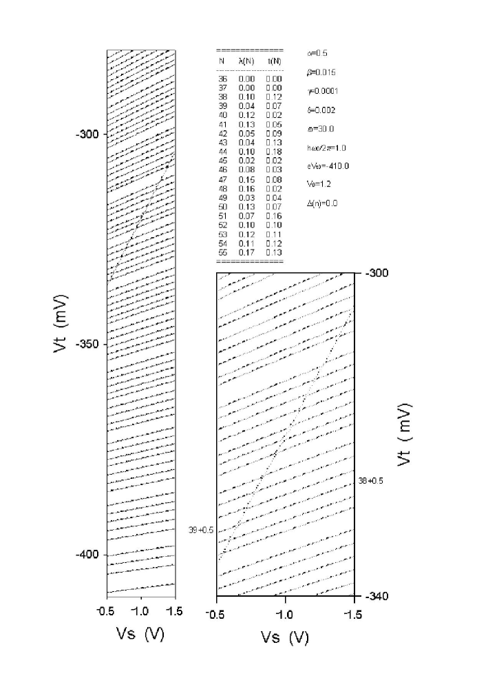
Figure 1: The plot of the electron addition energy versus the side gate voltage is shown. Zoom-in to the part near $V_{\mbox{t}}=-320\mbox{meV}$ is shown in the right. All quantities of energy dimension written in the right-top have the unit of meV. The dimensionless parameters $\alpha,~{}\beta,~{}\gamma,~{}\delta$ are chosen in order to obtain the similar feature of figure 1 (B) presented in Ref. 7. The values of $\Delta(n)$ related with $C(N_{\mbox{core}})$ is chosen simply as zero for all. The values of $\lambda(N)$ and $t(N)$ from $N=36$ to $55$ are arbitrarily given. A typical anomalous anticrossing takes place with $\lambda(39)<\lambda(38)$.

References

(1)R. C. Ashoori, H. L. Stormer, J. S. Weiner, L. N. Pfeiffer,
K. W. Baldwin, and K.W. West,
Phys. Rev. Lett.68, 3088 (1992).
(2)R. C. Ashoori, H. L. Stormer, J. S. Weiner, L. N. Pfeiffer,
K. W. Baldwin, and K.W. West,
Phys. Rev. Lett.71, 613 (1993).
(3)N. B. Zhitenev, R. C. Ashoori, L. N. Pfeiffer, and K.W. West,
Phys. Rev. Lett.79, 2308 (1997).
(4)Y. Wan, G. Ortiz, and P. Phillips, Phys. Rev. Lett.75, 2879 (1995).
(5)M. E. Raikh, and L. I. Glazmane, Phys. Rev. Lett.77, 1354 (1996).
(6)A. A. Koulakov, and B. I. Shklovskii, Phys. Rev.B57,
2352 (1998).
(7)N. B. Zhitenev, M. Brodsky, R. C. Ashoori, L. N. Pfeiffer, and K.W. West,
Science285, 715 (1999).
(8)D. Yoshioka, B. I. Halperin, and P. A. Lee, Phys.
Rev. Lett.50, 1219 (1983).
(9)M. H. Chung, J. Hong, and J. H. Kwon, Phys. Rev.B55,
2249 (1997).
(10)V. Fock, Z. Phys.47, 446 (1928).
(11)G. Arfken, Mathematical Methods for Physicists 2nd Ed.
(Academic Press, New York, 1970), p. 620.