Static Charge Coupling of Intrinsic Josephson Junctions

Abstract

A microscopic theory for the coupling of intrinsic Josephson oscillations due to charge fluctuations on the quasi two-dimensional superconducting layers is presented. Thereby in close analogy to the normal state the effect of the scalar potential on the transport current is taken into account consistently. The dispersion of collective modes is derived and an estimate of the coupling constant is given. It is shown that the correct treatment of the quasiparticle current is essential in order to get the correct position of Shapiro steps. In this case the influence of the coupling on dc-properties like the $I-V$-curve is negligible.

Pacs: 74.72.-h,74.80.Fp,74.50.+r,74.40.+k
Keywords: layered superconductors, intrinsic Josephson effect, SN-junction, Shapiro Steps

(Proceedings of HTS Plasma 2000 Symposion, Sendai August 22-24 2000, to appear in Physica C)

1 INTRODUCTION

Since the discovery of the intrinsic Josephson effect not only the typical properties of conventional junctions were demonstrated [1], but also unique and surprising features like the coupling of Josephson oscillations to phonons [2] have been discovered. There has also been a considerable interest in the influence of nonequilibrium effects on the $I-V$-characteristic and collective modes [3, 4, 5, 6, 7, 8, 9], as the quasi two-dimensional superconducting layers are expected to be more sensitive to external perturbations than bulk materials. Recent measurements of Shapirosteps on the resistive branch [10, 11] suggest to study the role of non-equilibrium effects on these, as the in depth theoretical understanding of this problem is important for any high-precision applications of high temperature superconductors (HTSC) as a voltage standard.

This paper is organized as follows: The microscopic theory for the electronic transport between the superconducting layers is developed and the close analogy of the static case to the normal state is pointed out. Then the consequences for the $I$-$V$-curve, the dispersion of collective modes and the position of Shapiro steps are being discussed. Further technical details can be found in [7, 8] and in a forthcoming publication [12].

2 TUNNELING THEORY

We consider a stack of $N+1$ (superconducting) layers $l=0,1,\dots,N$ forming $N$ intrinsic (Josephson) junctions in the homogeneous case. The normal conducting electrodes attached at the top and bottom of the stack in a 2-point measurement are denoted as $l=-1,N+1$ (cf. Fig. 1).

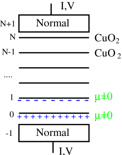
Figure 1: Schematic picture of the mesa of superconducting layers in a 2-point measurement.

As a motivation for the following discussion let us first recall the situation in the normal state. There the electrical current (density)

$$j_{l,l+1}^{NN} = {\sigma_{l,l+1}\over ed}(\mu_{l+1}^{\rm ec}-\mu_{l}^{\rm ec})$$ (1)

$$= \sigma_{l,l+1}E_{l,l+1}+{\sigma_{l,l+1}\over ed}(\mu_{l+1}^{c}-\mu_{l}^{c})$$ (2)

between the layers $l$ and $l+1$ is given by the difference of the electrochemical potentials $\mu_{l}^{ec}=\mu^{c}_{l}-eA_{0,l}$ (Fermi energy) in neighbouring layers ($d$ distance of layers, $e=|e|$). This can be separated in a diffusion term driven by the difference $\Delta^{(1)}\mu^{c}_{l}:=\mu_{l+1}^{c}-\mu_{l}^{c}$ of the chemical potentials $\mu_{l}^{c}$ and a field term $\sigma_{l,l+1}E_{l,l+1}=\sigma_{l,l+1}(A_{0,l}-A_{0,l+1})$.

In turn, the (static) charge fluctuation

$$\rho_{l,N}=-2eN_{2d}\mu_{l}^{c}$$ (3)

on the layer $l$ is determined completely by the filling of the conduction band or the chemical potential $\mu_{l}^{c}$ respectively. Using this and the Poisson equation ($\epsilon_{\infty}$: background dielectric constant)

$$\rho_{l}=\epsilon_{0}\epsilon_{\infty}\left(E_{l,l+1}-E_{l-1,l}\right)$$ (4)

$\mu_{l}^{c}$ can be eliminated from equ. 2:

$$j=j_{l,l+1}^{NN}=\sigma_{l,l+1}\left(1-\alpha_{0}\Delta^{(2)}\right)E_{l,l+1}$$ (5)

with the discrete derivative $\Delta^{(2)}f_{l}:=f_{l+1}+f_{l-1}-2f_{l}$ and the coupling constant

$$\alpha_{0}=\frac{\epsilon_{0}\epsilon}{2e^{2}dN_{2d}}\ll 1\quad.$$ (6)

For a fixed dc-bias current $j$ equ. 5 can be used to determine the electric field $E_{l,l+1}$ by applying the operator $1+\alpha_{0}\Delta^{(2)}$ on equ. 5. If all conductivities $\sigma_{l,l+1}$ are equal, no charge fluctuations accumulate and $E_{l,l+1}=j/\sigma$, while in the case of only one barrier with a higher resistance (e.g. $\sigma_{0,1}\ll\sigma_{l,l+1},l\neq 0$ ) the electric field is not only localized at the highly resistive junctions, but is spread to neighboring junctions

$$E_{0,1} = (1-2\alpha_{0})j/\sigma_{0,1}\quad,$$ (7)

$$E_{-1,0} = E_{1,2}=\alpha_{0}j/\sigma_{0,1}\quad.$$ (8)

In the superconducting state both the electric field $E_{l,l+1}$ and the difference ($l=0,\dots,N-1$)

$$\gamma_{l,l+1}=\chi_{l}-\chi_{l+1}-\frac{2e}{\hbar}\int_{l}^{l+1}A_{z}(z,t)dz$$ (9)

of the phases $\chi_{l}$ of the superconducting order parameters $\Delta_{l}=|\Delta_{l}|e^{i\chi_{l}}$ in neighboring layers are gauge invariant quantities and have an independent physical meaning. Its time derivative directly leads to the general Josephson relation

$$\frac{\hbar}{2e}{\dot{\gamma}}_{l,l+1}(t)=V_{l,l+1}+\mu_{l+1}-\mu_{l}\quad l=0,.,N-1$$ (10)

between the phase $\gamma_{l,l+1}$ and the voltage $V_{l,l+1}=d_{l,l+1}E_{l,l+1}$ across the junction, where the scalar potential $\mu_{l}$ is given by:

$$\mu_{l}=A_{0,l}-\frac{\hbar}{2e}{\dot{\chi}}_{l}(t)\quad\quad l=0,1,\dots,N\quad.$$ (11)

As can be seen from the Gorkov equation for the single particle Greens function, the static part $\mu_{l}^{\rm dc}/e$ plays the role of the chemical potential $\mu_{l}^{c}$ in the superconducting state.

In addition to this, a tunneling Hamiltonian

$$H_{T}=\sum_{l{\bf r}\sigma}t_{{\bf r}}^{\phantom{\ast}}c^{\dagger}_{l+1{\bf r}\sigma}c^{\phantom{\dagger}}_{l{\bf r}\sigma}e^{-i\frac{e}{\hbar}\int_{l}^{l+1}A_{z}(z,t)\,dz}+c.c.$$ (12)

between the (BCS-like) superconducting layers has to be specified explicitly in order to calculate $j_{l,l+1}$. In the following we will assume a hopping matrix element $t_{{\bf k}{\bf k}^{\prime}}^{2}=t_{s}^{2}+t_{d}^{2}g_{{\bf k}}g_{{\bf k}^{\prime}}$, which has both a constant $s$ and $d$-wave (i.e. $g_{{\bf k}}$) part in order to get both a Josephson current and a finite quasiparticle conductivity at the same time. The general structure of the theory will be independent of this choice.

A time dependent perturbation theory up to the second order in the hopping matrixelement $t_{{\bf k}{\bf k}^{\prime}}$ is performed, but no assumption for the external electromagnetic potentials $A_{0.l}(t)$ and $A_{z}(t)$ is made. The resulting expressions for the tunnel current

$$j_{l,l+1}={\Im}\sum_{\pm}\int\limits_{\infty}^{t}dt^{\prime}P_{\pm}(t,t^{\prime})e^{\frac{i}{2}(\gamma_{l,l+1}(t)\pm\gamma_{l,l+1}(t^{\prime}))}$$ (13)

between the layers $l$ and $l+1$ and the charge fluctuation

$$\rho_{l} = -\chi_{\rho\rho}\mu_{l}+Q_{t^{2}}(t,\gamma_{l,l+1})$$ (14)

on layer $l$ are nonlinear in $\gamma_{l,l+1}$. Thereby $\chi_{\rho\rho}$ is the charge suszeptibility of the superconducting layer, which is for $\omega=0$ connected with the two dimensional density of states $N_{\rm 2d}$ and independent of temperature $T$: $\chi_{\rho\rho}(\omega=0,T)=2e^{2}N_{\rm 2d}$. The correlation functions $P_{\pm}$ and the charge contribution $Q_{t^{2}}$ in $O(t_{{\bf k}{\bf k}^{\prime}}^{2})$ also depend on the scalar potential $\mu_{l}$ and have been expressed by Feynman diagrams in [7, 8].

Using the general ansatz for the phase

$$\gamma_{l,l+1}=\gamma_{0l}+\Omega_{l}t+\delta\gamma_{l,l+1}(t)$$ (15)

in resistive ($\Omega_{l}\neq 0$) and superconducting ($\Omega_{l}\neq 0$) junctions, $j_{l,l+1}$ and $\rho_{l}$ can be linearized in the (small) oscillations $\delta\gamma_{l,l+1}$ and the scalar potential $\mu_{l}$:

$$j_{l,l+1} = j_{c}\sin\gamma_{l,l+1}+\frac{\hbar\sigma_{0}}{2ed}\dot{\gamma}_{l,l+1}-\sigma_{1}\frac{1}{d}\Delta^{(1)}\mu_{l}$$ (16)

$$= j_{\l,l+1}^{\rm sup}\!+\!\sigma_{0}E_{l,l+1}\!+\frac{(\sigma_{0}-\sigma_{1})}{d}\Delta^{(1)}\mu_{l},$$

$$\rho_{l} = -\chi_{\rho\rho}\mu_{l}+\frac{i\sigma_{2}}{d\omega}\,\Delta^{(2)}\mu_{l}-\frac{\hbar\sigma_{1}}{2ed}\,\Delta^{(1)}\gamma_{l-1,l}$$ (17)

$$= -\chi_{\rho\rho}\mu_{l}+\frac{i}{\omega}\left(j_{l,l+1}^{Q}-j_{l-1,l}^{Q}\right)\quad,$$

$$j^{Q}_{l,l+1} = \sigma_{1}E_{l,l+1}+\frac{\left(\sigma_{1}-\sigma_{2}\right)}{d}\left(\mu_{l+1}-\mu_{l}\right)\;.$$ (18)

Here we restricted the discussion to a linear quasiparticle characteristic for simplicity. The conductivities $\sigma_{i}(\Omega_{l},\omega)$ will in general depend on both $\hbar\Omega_{l}/2e=V_{\rm dc}+\mu_{l+1}^{\rm dc}-\mu_{l}^{\rm dc}$ and the oscillation frequency $\omega$ of $\delta\gamma_{l,l+1}$, which coincides with $\Omega$ e.g. on the autonomous first resistive branch. Products like $(\sigma_{0}E_{l,l+1})(t)=\int\sigma_{0}(t-t^{\prime})E_{l,l+1}(t^{\prime})dt^{\prime}$ are to be interpreted as a folding in time space.

All conductivities $\sigma_{i}$ are of the same order of magnitude as the experimental quasiparticle conductivity $\sigma_{\rm exp}\approx 2(k\Omega{\rm cm})^{-1}$ (Bi-2212) and consequently corrections $\sigma_{i}/\epsilon_{0}\omega\ll 10^{-2}$ are small for frequencies $\omega>\omega_{\rm pl}$ on the resistive branch. The conductivity $\sigma_{1}$ is presented for different values of $\Omega$ in fig. 2. There the transition to the conductivity $\sigma_{N}=4e^{2}\pi N_{\rm 2d}t_{s}^{2}/\hbar^{3}$ for $\omega>2e\Delta_{0}$ ($\Delta_{0}$: maximal $d$-wave gap) and the slight difference between the value of $\sigma_{1}$ in a superconducting and a resistive junction can be seen. The negative part for small frequencies is not a violation of causality, but arises from the fact that $\sigma_{1}$ is not a conventional transport coefficient.

The static limit of $\sigma_{1}$ is subtle and deserves special attention. Formally the result for $\omega=0$ cannot be obtained in our formalism by expanding $\rho_{l}$ or $j_{l,l+1}$ in the static part $\mu_{l}^{\rm dc}$ of the scalar potential directly. Instead of this the static inhomogenity has to be included in the equilibrium Greens function in zeroth order in $t_{{\bf k}{\bf k}^{\prime}}$. For $\omega\rightarrow 0$ and $T<eV\ll\Delta_{0}$ one gets the finite value

$$\sigma_{1}(\Omega,\omega\rightarrow 0)\sim\sigma_{N}\frac{T}{\Delta_{0}}\frac{eV}{\Delta_{0}}\quad,$$ (19)

while the strictly static function $\sigma_{1}^{\rm dc}:=\sigma_{1}(\omega=0,T)=0$ vanishes exactly for all temperatures. This discontinuity is due to the fact that our only relaxation mechanism is the incoherence of the hopping $t_{{\bf k}{\bf k}^{\prime}}$ between layers. Therefore in a tunneling process (which is already of order $t_{{\bf k}{\bf k}^{\prime}}^{2}$) no additional relaxation within the layers is possible, if we work strictly in $O(t_{{\bf k}{\bf k}^{\prime}}^{2})$. Including strong impurity scattering in the layers, which is the main mechanism for charge imbalance relaxation in $d$-wave superconductors, leads to $\sigma_{1}(\omega\rightarrow 0)=\sigma_{1}(\omega=0)=0$ like in [5], which will be considered mainly in the following. It is pointed out that this choice is strictly speaking model dependent and a finite value $\sigma_{1}^{\rm dc}$ similar to our result for $\sigma_{1}(\omega\rightarrow 0)$ in equ. 19 could be obtained, if additional scattering mechanisms are considered.

Figure 2: Real and imaginary part of $\sigma_{1}$ in superconducting ($\Omega=0$, top figure) or resistive ($\Omega\neq 0$, bottom figure) junctions at $T=0$.

The elimination of $V_{\l,l+1}$, $\mu_{l}$ and $\delta\rho_{l}$ from equations 4, 10, 16 and 17 leads to a set of coupled equations of motion for the phases $\gamma_{l,l+1}$ ($\omega_{\rm pl}^{2}:=2edj_{c}/\hbar\epsilon_{0}$, $\omega_{c}=\omega_{\rm pl}^{2}\epsilon_{0}/\sigma_{0}$, $\Delta_{\alpha}^{(2)}:=1-\Delta^{(2)}\alpha$):

$$\frac{j}{j_{c}}=\Delta_{\alpha}^{(2)}\sin\gamma_{l,l+1}+\frac{1}{\omega_{c}}\Delta_{\eta}^{(2)}\dot{\gamma}_{l,l+1}+\frac{1}{\omega_{\rm pl}^{2}}\Delta_{\zeta}^{(2)}\ddot{\gamma}_{l,l+1}$$

The coupling constants are given as:

$$\alpha(\omega) := \frac{\epsilon_{0}\epsilon}{d\chi_{\rho\rho}}\left(1+\frac{i\sigma_{2}}{\epsilon_{0}\epsilon\omega}\right)\quad,$$ (20)

$$\eta(\omega) := \frac{\epsilon_{0}\epsilon}{d\chi_{\rho\rho}}\left(1+\frac{i\sigma_{2}}{\epsilon_{0}\epsilon\omega}-\frac{2\sigma_{1}}{\sigma_{0}}\right)\quad,$$ (21)

$$\zeta(\omega) := -\frac{\epsilon_{0}\epsilon}{d\chi_{\rho\rho}}\frac{i\sigma_{2}}{\epsilon_{0}\epsilon\omega}.$$ (22)

These are in the static case completely determined by the normal state value in equ. 6: $\alpha(\omega=0)=\eta(\omega=0)=\alpha_{0}$ and $\zeta(\omega=0)=0$.

The rough theoretical estimate for $\alpha_{0}\approx 0.28$ (for $\epsilon=10$, $d=1.5{\rm nm}$) based on a twodimensional electron gas with density of states $N_{\rm 2d}=m_{\rm el}/2\pi^{2}\hbar^{2}$ (not including spin) is to be considered as an upper bound, as the density of states at the Fermi surface could be enhanced by a factor 2-3 due to strong electronic correlations [13]. A more reliable estimate $\alpha\approx 0.2$ is possible from optical experiments and will be elaborated in detail elsewhere [14].

Linearizing the set of equations 2 one obtains the dispersion of collective modes (in order $O(t_{{\bf k}{\bf k}^{\prime}}^{2})$, $\omega_{0}:=\sigma_{0}/\epsilon_{0}\epsilon=\omega_{\rm pl}^{2}/\omega_{c}$, $\overline{\omega}_{\rm pl}^{2}=\omega_{\rm pl}^{2}/\epsilon_{c}^{\infty}$):

$$\omega^{2} \stackrel{{\scriptstyle k_{z}\ll 1}}{{\approx}} \overline{\omega}_{\rm pl}^{2}\;\frac{1+\alpha k_{z}^{2}}{1+\zeta k_{z}^{2}}-i\omega\omega_{0}\;\frac{1+\eta k_{z}^{2}}{1+\zeta k_{z}^{2}}=$$ (23)

$$= \overline{\omega}_{\rm pl}^{2}\left(1+\alpha k_{z}^{2}\right)-i\omega\omega_{0}\left(1+\eta k_{z}^{2}\right)\quad.$$ (24)

For frequencies $\omega_{\rm pl}\ll\omega\ll\Delta_{0}$ on the resistive branch these represent weakly damped plasma modes of the superconducting condensate. For the special case $e\rightarrow 0$ the dispersion $\omega(k_{z})\rightarrow 0$ for $k_{z}\rightarrow 0$ of the Goldstone mode associated with the spontaneous breaking of the gauge symmetry in the superconducting state can be obtained explicitly. This reproduces in the Kuboformalism the results in [5, 6], which were obtained by solving kinetic equations.

Figure 3: Real and imaginary part of $\alpha(\omega)$ for $d$-wave pairing for temperature $T=0$ in $O(t_{{\bf k}{\bf k}^{\prime}}^{0})$ ($\omega$ in units $\Delta_{0}(T)$, $\epsilon_{\infty}={\rm const.}$).

Taking into account only the leading order $O(t_{{\bf k}{\bf k}^{\prime}}^{0})$ in the hopping matrix element, $\alpha(\omega,T)$ has been calculated in [7] and is presented for $T=0$ in fig. 3. This result is obtained for a constant background dielectric constant $\epsilon$, while the frequency dependence of $\epsilon_{\infty}(\omega)$ near phonon resonances can change the behaviour of $\alpha(\omega)$ considerably [2]. For the temperature dependence see [8].

We would like to point out the remarkable similarity of the static quasiparticle current in the superconducting and in the normal state. Due to $\sigma_{1}(\omega=0)=0$ equ. 16 reduces to:

$$j_{\rm dc}=j_{c}\langle\sin\gamma_{l,l+1}\rangle+\frac{\hbar\sigma_{0}}{2ed}\langle{\dot{\gamma}}_{l,l+1}\rangle+\langle\frac{\sigma_{1}}{d}(\mu_{l+1}-\mu_{l})\rangle$$

In the last term of equ. 2 the static part of $\mu$ does not contribute due to $\sigma_{1}(\Omega,\omega=0)=0$, but a finite dc-contribution might arise from the combination of $\mu(\Omega)$ and Josephson-like terms in $\sigma_{1}$. This term is in intrinsic junctions negligible of order $\alpha t_{{\bf k}{\bf k}^{\prime}}^{4}\ll 1$ and vanishes exactly for SN-junctions:

$$j_{\rm dc} = \left(\langle j_{l,l+1}^{\rm sup}\rangle+\langle j_{l,l+1}^{NN}\rangle\right)=$$ (25)

$$= j_{c}\langle\sin\gamma_{l,l+1}\rangle+\frac{\hbar\sigma_{0}}{2ed}\langle{\dot{\gamma}}_{l,l+1}\rangle=$$ (26)

$$= j_{c}\langle\sin\gamma_{l,l+1}\rangle+\sigma_{0}\Delta_{\alpha_{0}}^{(2)}E_{l,l+1}^{\rm dc}$$ (27)

where the quasiparticle current coincides with equ. 2, if we express $\gamma_{l,l+1}$ by $E_{l,l+1}$ and $\mu_{l}$ via equ. 10 The dc-equations

$$j = \sigma_{0}^{SN}E_{N,N+1}+\left(\sigma_{0}^{SN}-\sigma_{1}^{SN}\right)\Delta^{(1)}\mu_{N}=$$ (28)

$$= \sigma_{0}^{SN}\left((1+\alpha_{0}^{\prime})E_{N,N+1}-\alpha_{0}^{\prime}E_{N-1,N}\right),$$

$$j = \sigma_{0}^{SN}\left((1+\alpha_{0}^{\prime})E_{-1,0}-\alpha_{0}^{\prime}E_{0,1}\right)$$ (29)

for the SN-junctions are slightly different, as the change of the chemical potential $\mu_{-1}^{c}=\mu^{c}_{N+1}=0$ in bulk materials is negligible due to the large density of states. Thereby $\alpha_{0}^{\prime}=\alpha_{0}(1-\sigma_{1,SN}^{rmdc}/\sigma_{0,SN}^{\rm dc})$, which is in the model with strong impurity scattering in the layers given as: $\alpha_{0}^{\prime}=\alpha_{0}$.

If we neglect the supercurrent for a moment, the inversion of the operator $\Delta_{\alpha_{0}}^{(2)}$ shows that the total voltage $V^{\rm dc}=\sum_{i=-1}^{N}V_{l,l+1}^{\rm dc}$ is exactly given like in a stack of independent junctions, i.e. the coupling constant $\alpha_{0}$ does not enter in the $I$-$V$-curve. The dc-component of the supercurrent might add a correction to this due to the interaction $\alpha$ at the frequency $\Omega$, but this contribution is suppressed by a factor $t_{{\bf k}{\bf k}^{\prime}}^{2}\alpha_{0}\ll 1$ and therefore no significant effect on dc-properties are expected.

It is pointed out that this general result cannot be obtained by assuming an ohmic quasiparticle current $j^{\rm qp}_{l,l+1}=\sigma E_{l,l+1}$ as in [3]. An additional indication that the correct choice of the quasiparticle current is essential will come from the discussion of Shapiro steps in the next section.

This might also be the reason that up to now no clear experimental evidence for the coupling $\alpha$ in the $I$-$V$-characteristic, like small deviations in the additivity of resistive branches [8], could be found.

Nevertheless, the distribution of the electric fields $E_{l,l+1}^{\rm dc}$ within the stack is affected by the coupling $\alpha_{0}$ like in equ. 7 and 8 in the normal state. For a single resistive junction the electric field is not contained in this junction, but leaks into neighboring junctions in the same way as around a junction with much lower resistance in a stack of normal junctions.

It is stressed that the above discussion makes use of the fact that $\sigma_{1}^{\rm dc}=0$ in the presence of strong impurity scattering in the layers. In a more general model this might not be the case and coupling terms $\sim\alpha_{0}\sigma_{1}^{\rm dc}/\sigma_{0}^{\rm dc}$ appear.

The coupling via charge fluctuations might also have a considerable effect at frequencies larger than the charge imbalance relaxation rates (e.g. for phaselocking at microwave frequencies), where the $\sigma_{1}/\sigma_{0}$ in equ. 21 can be of order $O(1)$ in any model.

3 SHAPIRO STEPS

A Shapiro step is generated by microwave irradiation of frequency $\Omega$, which creates an oscillating component of the $c$-axis bias current $I_{\rm ac}=I_{\rm rf}\sin(\Omega t)$. Thereby the dynamics of the phase in a resistive junction is given as

$$\gamma_{n,n+1}(t)=\gamma_{0n}+\Omega t+\gamma_{1n}\sin(\Omega t)\quad.$$ (30)

Therefore the supercurrent ($J_{k}$: Bessel functions of first kind)

$$I_{\rm supra} = I_{c}\sin\left(\gamma_{n.n+1}(t)\right)=$$

$$= I_{c}\sum_{k=-\infty}^{\infty}J_{k}(\gamma_{n1})\sin\left(\gamma_{n0}+(1+k)\Omega t\right)$$

has a dc component

$$I_{\rm supra}^{\rm dc}=I_{c}J_{-1}(\gamma_{1n})\sin(\gamma_{0n})\quad,$$ (32)

which creates the (first) Shapiro step in the $I$-$V$-curve.

The nontrivial question in the following will be, what dc-voltage $V_{\rm step}$ is connected with a given $\Omega$, if the generalized Josephson relation equ. 10 is taken into account. Using equation 4 and 17 this can be presented as:

$$\frac{\hbar}{2ed}{\dot{\gamma}}_{l,l+1}=(1+2\alpha)E_{l,l+1}-\alpha\left(E_{l-1,l}+E_{l+1,l+2}\right)$$ (33)

for $l=0,\dots,N-1$. This set of $N$ equations is not sufficient to determine all $N+2$ voltages $V_{l,l+1}$ and has to be complemented by the current equations 28 and 29 in the SN-junctions.

Note that for the total voltage $V_{\rm step}$ across the stack the transport coefficients in the intrinsic Josephson junctions are irrelevant.

In the ”superconducting” state, which is defined by $\langle{\dot{\gamma}_{l,l+1}}\rangle=0$ for all $l=0,\dots,N-1$, one easily obtains (in $O(\alpha_{0}^{\prime})$)

$$E_{-1,0}^{\rm dc} = E_{N,N+1}^{\rm dc}=\left(1-\alpha_{0}^{\prime}\right)j/\sigma_{0,SN}\quad,$$ (34)

$$E_{l,l+1}^{\rm dc} = 0\quad\quad l=1,\dots,N-2\quad,$$ (35)

$$E_{0,1}^{\rm dc} = E_{N-1,N}^{\rm dc}=-\alpha_{0}^{\prime}j/\sigma_{0,SN}^{\rm dc}$$ (36)

and the total dc-voltage

$$V^{\rm dc}=\sum_{l=-1}^{N}V_{l,l+1}^{\rm dc}=\frac{2jd}{\sigma_{0,SN}^{\rm dc}}$$ (37)

This linear branch reflects the contact resistances at both SN-junctions and is not affected by the coupling $\alpha_{0}^{\prime}$, although the voltages $V_{l,l+1}$ in the intrinsic junctions in general do not vanish.

For a single resistive junction in the top layer $l=N-1$ ($\langle{\dot{\gamma}}_{N-1,N}\rangle=\Omega$, $\langle{\dot{\gamma}}_{n,n+1}\rangle=0$, $n$ else) one obtains analogously:

$$E_{N,N+1} = (1-\alpha_{0}^{\prime})j/\sigma_{0,SN}^{\rm dc}+\alpha_{0}^{\prime}\frac{\hbar\Omega}{2ed}+O(\alpha_{2}^{\prime 2}),$$

$$V_{\rm step} = \frac{\hbar}{2e}\Omega\left(1-\alpha_{0}\frac{\sigma_{1,SN}^{\rm dc}}{\sigma_{0,SN}^{\rm dc}}\right)\stackrel{{\scriptstyle\sigma_{1,SN}^{\rm dc}=0}}{{=}}$$ (38)

$$= \frac{\hbar}{2e}\Omega$$ (39)

The last result is correct in all orders of $\alpha_{0}^{\prime}$. Here the dc-conductivity $\sigma^{\rm dc}_{1,SN}=0$ has been kept explicitly in equ. 38 in order to demonstrate that the position of the step in general depends on the value of $\sigma_{1,SN}^{\rm dc}$. In the model considered here $\sigma_{1,SN}^{\rm dc}=0$ and the Shapiro step is where expected, which would not be obtained by using the ohmic quasiparticle current alone ($\sigma_{0,SN}^{\rm dc}=\sigma_{1,SN}^{\rm dc}$) like in [3]. Nevertheless this result opens up the principal possibility that there is a shift in the position of the Shapirostep in a more general theory (e.g including electron-phonon scattering) due to nonequilibrium effects, where $\sigma_{1}^{\rm dc}$ might not vanish. Taking out result equ. 19 seriously the relative shift would be small $\sim 10^{-5}$, but detectable.

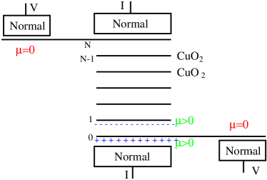
Figure 4: Schematic 4-point geometry by [15]

This result is also valid in a 4-point measurement geometry, as sketched in Fig. 4 and used by [15]. Although the total voltage

$$V_{\rm step}^{\rm int}=\sum_{l=0}^{N-1}V_{l,l+1}^{\rm dc}=\frac{\hbar\Omega}{2e}\left(1-\alpha_{0}\right)+\frac{2j\alpha_{0}}{\sigma_{0,SN}^{\rm dc}}$$ (40)

across the intrinsic contacts depends on $\alpha_{0}$, this deviation of the expected position of the Shapiro step cannot be detected at the contacts. The electrochemical potential is constant along the superconducting layers, but the potential $\mu_{l}(x)$ and the electric field $E_{\parallel}$ are not and will compensate the additional contribution in equ. 40. Also in the non equilibrium theory of [9] there is no shift of Shapiro steps.

Finally, note that all the above considerations only apply to an experimental situation where the electric field $E^{\rm dc}$ is measured directly to determine the dc-voltage $V^{\rm dc}$. This might not be operational with conventional voltmeters, which actually detect a current through a circuit with high resistance, which is driven by the difference of the electrochemical potentials $\mu_{l}^{\rm ec}$ rather than the voltage $V^{\rm dc}$ [16].

4 CONCLUSIONS

The microscopic theory of tunneling in layered superconductors has been studied including the effect of the scalar potential on the layers and an estimate of the coupling constant $\alpha\approx 0.2$ has been given from optical experiments. The static quasiparticle current includes both field and diffusion terms as in the normal state, which turns out to be crucial for all dc properties. In the model with strong impurity scattering in the layers, Shapiro steps are exactly at the expected position $V_{\rm step}=\hbar\Omega/2e$. In this case the effect of charging on the total $I$-$V$-curve is suppressed by a factor $\alpha_{0}t_{{\bf k}{\bf k}^{\prime}}^{2}$ and therefore negligible, but it affects the distribution of the electric field within the stack.

This results motivate the study of more general microscopic models including different relaxation mechanisms like electron-phonon scattering, as a finite $\sigma_{1}^{\rm dc}$ would modify the position $V_{\rm step}$ in a characteristic way with important consequences for potential applications as a voltage standard. Also precision experiments on Shapiro steps could then be used as a sharp test for microscopic theories.

The authors would like to thank S. Rother, R. Kleiner and P. Müller for discussing their unpublished experimental data and L.N. Bulaevskii for his interest in this work. Financial support by DFG, FORSUPRA and DOE under contract W-7405-ENG-36 (C.H.) is gratefully acknowledged.

References

- [1] R. Kleiner, F. Steinmeyer, G. Kunkel, P. Müller, Phys. Rev. Lett. 68 (1992), 2394; R. Kleiner, P. Müller, Phys. Rev. B 49 (1994), 1327.
- [2] Ch. Helm, Ch. Preis, F. Forsthofer, J. Keller, K. Schlenga, R. Kleiner, P. Müller, Phys. Rev. Lett. 79 (1997), 737.
- [3] T. Koyama, M. Tachiki, Phys. Rev. B 54, 22 (1996) 16183.
- [4] S.N. Artemenko, A.G. Kobelkov, Phys. Rev. Lett. 78, 18 (1997) 3551; S.N. Artemenko, JETP Letters 70, 8 (1999), 526.
- [5] S.N. Artemenko, A.G. Kobelkov, Phys. Rev. B 55, 14,(1997) 9094; JETP Letters 65, 4, (1997) 331.
- [6] S.N. Artemenko, A. G. Kobelkov, Physica C 253 (1995), 373.
- [7] C. Helm, Intrinsischer Josephsoneffekt und Phononen, Ph.D. thesis, University of Regensburg, Germany,1998.
- [8] Ch. Preis, Ch. Helm, J. Keller, A. Sergeev, R. Kleiner, SPIE Conference Proceedings Vol 3480, San Diego, (1998), 236.
- [9] D. A. Ryndyk, JETP Lett. 65, 10 (1997), 791; D. A. Ryndyk, Phys. Rev. Lett. 80, 15 (1998), 3376; D. A. Ryndyk, JETP 89, 5 (1999), 975.
- [10] S.Rother, R.Kleiner, P.Müller, M.Darula, Y.Kasai, K.Nakajima, Physica C.
- [11] Y.-J. Doh, J. Kie, K.-T. Kim, H.-J. Lee, Phys. Rev. B 61, 6 (2000), R3834.
- [12] Ch. Helm, J. Keller, Ch. Preis, A. Sergeev, S. Shafranjuk, in preparation.
- [13] E. Dagotto, Rev. of Mod. Phys. 66, 3 (1994), 763; D. S. Dessau, Z. X. Shen, D. M. King, D. S. Marshall, Phys. Rev. Lett. 71 (1993), 2781.
- [14] L.N. Bulaevskii, Ch. Helm, in preparation.
- [15] Y.I. Latyshev, S.J. Kim, T. Yamashita, JETP Letters , 69,8 (1999) 640.
- [16] D. E. McCumber, Phys. Rev. Lett. 23, 21 (1969) 1228.