Phase Diagram of Bilayer Composite Fermion States

Abstract

We construct a class of composite fermion states for bilayer electron systems in a strong transverse magnetic field, and determine quantitatively the phase diagram as a function of the layer separation, layer thickness, and electron density. We find, in general, that there are several transitions, and that the incompressible phases are separated by compressible ones. The paired states of composite fermions, described by Pfaffian wave functions, are also considered.

I Introduction

Multicomponent fractional quantum Hall effect is of relevance to situations when there exists more than one species of electron, distinguished by, for example, their spin or the layer index. There has been substantial interest in multicomponent states of fractional quantum Hall effect (FQHE) in recent years both because of their experimental realizations, and because of theoretical progress in the understanding of their structure. The focus in this article will be on multicomponent states in a bilayer system. For simplicity, we will assume that the Zeeman energy is sufficiently large that the electron spin is completely frozen, which is a good approximation in the limit of large magnetic fields.

Multicomponent FQHE states were first considered in 1984, when Halperin[1] generalized Laughlin’s wave function for the $\nu=1/3$ FQHE [2] to states containing more than one component of electron:

$$\chi {}_{m^{\prime},m^{\prime\prime},m}[\{z_{i}\},\{w_{r}\}]=\prod_{j<k=1}^{N_{1}}(z_{j}-z_{k})^{m^{\prime}}$$ (1)

$$\times \prod_{r<s=1}^{N_{2}}(w_{r}-w_{s})^{m^{\prime\prime}}\prod_{j,r}(z_{j}-w_{r})^{m}$$ (2)

$$\times \exp[-\frac{1}{4}(\sum_{j=1}^{N_{1}}|z_{j}|^{2}+\sum_{r=1}^{N_{2}}|w_{r}|^{2})]$$ (3)

Here, $z=x-iy$ and $w=x-iy$ denote the positions of the two components of electrons, labeled by subscripts $j,k$ and $r,s$. The exponents $m^{\prime\prime}$ and $m^{\prime}$ are odd integers, to ensure proper antisymmetry, and $m$ is an arbitrary integer. $N_{1}$ and $N_{2}$ are the numbers of electrons in the two layers.

These wave functions were first applied to mixed spin FQHE states, i.e., when electrons with both spins are relevant. (Such a possibility arises in GaAs because the Zeeman splitting is much smaller than the characteristic Coulomb interaction energy for typical parameters.) The function $\chi_{m^{\prime},m^{\prime\prime},m}$ is only the spatial part; the full wave function is given by

$$A[\chi_{m^{\prime},m^{\prime\prime},m}[\{z_{i}\},\{w_{r}\}]\;u_{1}u_{2}...u_{N_{1}}d_{1}d_{2}...d_{N_{2}}]$$ (4)

where $A$ is the antisymmetrization operator and $u$ and $d$ are up and down spinors. When the inter-electron interaction is spin-independent, the ground state is an eigenstate of spin. Only the wave functions with a well defined spin quantum number are valid variational wave functions. (In principle, due to the spin-orbit coupling, other wave functions may also become relevant. However, the spin-orbit coupling is weak in GaAs and almost invariably neglected in theoretical considerations.) Some examples of states that have a well defined spin quantum number, i.e., satisfy the Fock condition are the fully polarized state $\chi_{1,1,1}$ at $\nu=1/3$ (it is identical to Laughlin’s fully polarized wave function except that the spin is pointing in the plane, giving zero z-component, rather than normal to the plane) and the spin-singlet state $\chi_{3,3,2}$ at $\nu=2/5$.

Later, the multicomponent wave functions were also considered for bilayer systems. The wave function in Eq. 4 also applies to bilayer systems, but with $u$ and $d$ playing the role of pseudospinors, indicating the occupation of the left and right layers, respectively. When the layer separation $d$ is zero, the problem is equivalent to that of spinful electrons in a single layer with the Zeeman energy set to zero, because the inter-electron interaction is pseudospin independent, given by

$$V^{2D}(r)=\frac{e^{2}}{\epsilon r}$$ (5)

independent of the layer index of the particles. In this limit, again only a limited class of the above wave functions has the correct symmetry. However, for finite $d$, the effective two-dimensional inter-electron interaction is explicitly pseudospin dependent: For electrons in the in the same layer, it is

$$V_{\uparrow\uparrow}(r)=V_{\downarrow\downarrow}(r)=\frac{e^{2}}{\epsilon r}$$ (6)

but for electrons in different layers, it is

$$V_{\uparrow\downarrow}(r)=\frac{e^{2}}{\epsilon\sqrt{r^{2}+d^{2}}}\;.$$ (7)

Here, $r$ is the projection of the distance in the plane and $\uparrow$ and $\downarrow$ denote the two layers. Thus, for finite $d$, none of the Halperin’s wave functions can be ruled out for symmetry reasons alone. The simplest non-trivial state is the state $\chi_{3,3,1}$, which describes an incompressible state at $\nu=1/2$. A FQHE at $\nu=1/2$ has indeed been observed[3, 4] in a certain range of layer separation in bilayer systems, believed to be well described by $\chi_{3,3,1}$[5]. (Note that the filling factor is defined to be the total filling; e.g., $\nu=1/2$ corresponds to a filling factor of $1/4$ in each individual layer.) Another interesting example is the QHE state $\chi_{1,1,1}$ at $\nu=1$. It is a non-trivial state for a bilayer system. For a single layer, $\nu=1$ QHE occurs even for non-interacting electrons, because a gap opens up due to Landau level quantization. For the bilayer system, however, the FQHE at $\nu=1$ originates due to interactions, as can be seen by noting that each layer has $\nu=1/2$, for which there is no gap for independent electrons. There is experimental evidence for this state also [6]. (Distinguishing the bilayer $\nu=1$ from the single layer $\nu=1$ is subtle, due to the unavoidable presence of some tunneling in the real experimental system, and a systematic study of the evolution of the state as a function of various parameters is necessary for its unambiguous identification. Further discussion and the relevant literature can be found in Ref. [7].) Recently, there has been a revival of interest in the $\nu=1$ bilayer state because of experimental observations [8] that have been interpreted in terms of a Josephson-like collective tunneling[9].

The physics of multicomponent FQHE states is expected to be intimately connected to and derived from the physics of the FQHE in single component systems. However, Laughlin’s wave function, which forms the basis of the states discussed above, describes only a subset of the observed states at $\nu=n/(2pn\pm 1)$ in a single layer system. The wave functions in Eq. 3 therefore also describe only a subset of a larger class of bilayer states. To take a simple example of states not described by $\chi_{m^{\prime},m^{\prime\prime},m}$, consider $m=0$, i.e., two uncoupled layers, and assume equal density in the two layers. The above wave function only applies to FQHE at $2/m^{\prime}$, with $m^{\prime}$ an odd integer, even though in reality FQHE will occur at a much larger class of fractions given by $\nu=2n/(2pn\pm 1)$. Further, Halperin’s wave functions are not applicable to compressible states, which, as we shall see, play an important role in the bilayer phase diagram.

The general theory of the FQHE in a single layer is formulated in terms of a particle called the composite fermion, which is the bound state of an electron and $2p$ quantum mechanical vortices[10]. The states of composite fermions are described by the wave function[10]

$$\psi_{n/(2pn+1)}={\cal P}_{LLL}\Phi_{n}\prod_{j<k}(z_{j}-z_{k})^{2p}$$ (8)

which is interpreted as $\nu^{*}=n$ filled Landau levels of composite fermions, $\nu^{*}$ being the filling factor of composite fermions. Here $\Phi_{n}$ is the wave function of $n$ filled Landau levels of electrons, and the Jastrow factor $\prod_{j<k}(z_{j}-z_{k})^{2p}$ attaches $2p$ vortices to each electron to convert it into a composite fermion [11]. The symbol ${\cal P}_{LLL}$ denotes the projection of the product wave function into the lowest electronic Landau level. These wave functions are known to be extremely accurate representations of the actual wave functions. Laughlin’s wave function is obtained for the special case $n=1$, and represents one filled composite-fermion Landau level. In the limit $\nu\rightarrow 1/2p$, the composite fermion filling factor approaches $n\rightarrow\infty$, i.e., the effective magnetic field experienced by the composite fermions, $B^{*}=\rho\phi_{0}/n$, vanishes. They form a Fermi sea here [12, 13], as confirmed experimentally[14]. In this limit, $\Phi_{\infty}$ becomes the wave function of a Fermi sea at zero magnetic field, and $\psi_{1/2p}$ describes a compressible Fermi sea of composite fermions. It is a remarkable feature of the composite fermion theory that it yields a description not only of all of the incompressible FQHE states, but also of the compressible liquids in the lowest Landau level.

The multicomponent generalization of the composite fermion theory for the mixed spin states in a single layer has been considered extensively in the past[15, 16, 17, 18]. The generalized wave functions are

$$\psi_{n/(2pn+1)}^{(n_{\uparrow},n_{\downarrow})}={\cal P}_{LLL}\Phi_{n_{\uparrow},n_{\downarrow}}\prod_{j<k}(z_{j}-z_{k})^{2p}$$ (9)

where $n=n_{\uparrow}+n_{\downarrow}$ and $z_{j}$ label all particles. Here, $n_{\uparrow}$ and $n_{\downarrow}$ are the numbers of occupied spin-up and spin-down composite-fermion Landau levels. This wave function satisfies the Fock conditions for all choices of $n_{\uparrow}$ and $n_{\downarrow}$, with each choice giving a FQHE state with a definite total spin, namely $(N/2)(n_{\uparrow}-n_{\downarrow})/(n_{\uparrow}+n_{\downarrow})$. In the limit of vanishing Zeeman energy, the ground state has the smallest total spin: the total spin is $S=0$ when $n$ is an even integer, with $n_{\uparrow}=n_{\downarrow}=n/2$; when $n$ is an odd integer, we have $n_{\uparrow}=(n+1)/2$ and $n_{\downarrow}=(n-1)/2$, with $S=N/2n$, $N$ being the total number of particles. As the Zeeman energy is increased, at certain critical values of the Zeeman energy $n_{\uparrow}$ increases by one unit while $n_{\downarrow}$ decreases by one unit. At very large Zeeman energies, a fully polarized state is obtained. This description is in excellent agreement with transport and optical experiments[19], and also with exact diagonalization studies on small systems[15]. It has also been extended to finite temperatures in a Hamiltonian formulation[17]. It ought to be noted that the wave functions $\psi_{n/(2pn+1)}^{(n_{\uparrow},n_{\downarrow})}$ describe only uniform liquid states; another structure, a charge/spin density waves of composite fermions, has been discussed in the context of certain experimental anomalies[20]. Halperin’s $\chi_{2p+1,2p+1,2p}$ state at $\nu=2/(4p+1)$ is obtained as a special case with $n_{\uparrow}=1$ and $n_{\downarrow}=1$; the other composite fermion (CF) states are not expressible in the form of a Halperin wave function.

Our objective in this work is to generalize the composite fermion theory to bilayer systems and determine the phase diagram of bilayer composite fermion states. The generalization of the composite fermion theory from single to two layers is, to an extent, straightforward, as we show below. Much work on possible bilayer states has been done in the past[21], but these studies do not tell us which states would actually occur in nature, and in what parameter range. Our goal is to obtain a quantitative description. We determine the phase diagram of composite fermion states as a function of two important parameters of the problem, the layer thickness $W$ and the layer spacing $d$ (defined to be the distance between the centers of the two layers). Due to its variational nature, the study cannot rule out other states, but we believe that the states considered here exhaust the physically relevant uniform liquid states in the parameter ranges considered. An important feature of the resultant phase diagram is that the incompressible CF phases are often separated by compressible phases; i.e., as a function of the inter-layer spacing, the transition typically occurs from a compressible state into an incompressible state, or vice versa. In general, several phase transitions are possible at a given fraction. Many of these phase transitions occur in presently accessible experimental regimes, and ought to be observable.

There has also been exact diagonalization work on two layer systems [22, 23, 24, 5]. It is restricted to extremely small systems, because of the drastically enlarged Hilbert space (compared to the single layer problem), and is therefore limited in its applicability. The exact diagonalization approach is also suitable only for incompressible states. Nonetheless, these studies provide indications regarding the range of parameters where some of the states, for example $\nu=1/2$ bilayer FQHE state, are strongest. Our results below are generally consistent with the earlier results. We also compare our results with available experiments at $\nu=1/2$ and $\nu=1$.

The plan of the paper is as follows. In the next section, we describe the generalization of the composite fermion theory to two layer system. Section III discusses the details of our computational method. In section IV, we display the quantitative phase diagram of bilayer CF states in the density-layer separation ($\rho-d$) plane for several quantum well thicknesses at total fillings $\nu=1/2,1/3,1,$ and $2/5$. In Section V our results are compared with exact diagonalization studies and experiment. Section VI considers bilayer CF states with Pfaffian structure in each layer. The paper is concluded in Section VII.

II Composite fermion theory for bilayer systems

In the case of a bilayer system, we already know the answer in two limits. When the layers are far apart, the bilayer state is given simply by two independent single-layer composite fermion states. In the other limit, when the layer separation $d\rightarrow 0$, the bilayer problem is identical to the problem of spinful electrons in a single layer (i.e., pseudospin acts like the real spin), with the Zeeman energy set equal to zero. Fortunately, as discussed above, the nature of the CF states is well understood in this limit. At even numerator fractions, the ground state is a (pseudo)spin singlet, and at odd numerator fractions it is partially polarized. For the pseudospin singlet state the densities in the two layers are equal; when the polarization is not zero, the densities depend on the direction of the total spin, with equal densities obtained when the total pseudospin is pointing parallel to the plane.

To investigate the intermediate situation, we consider the following class of wave functions which we expect to be particularly favorable energetically:

$$\Psi_{(\overline{\nu}_{1},\overline{\nu}_{2}|m)}=\prod_{r,j}(z_{j}-w_{r})^{m}\psi_{\overline{\nu}_{1}}[\{z_{k}\}]\psi_{\overline{\nu}_{2}}[\{w_{s}\}]$$ (10)

where the fully antisymmetric wave function $\psi_{\overline{\nu}}$ describes a lowest Landau level projected single layer state at filling factor $\overline{\nu}$. The state described by $\Psi_{(\overline{\nu}_{1},\overline{\nu}_{2}|m)}$ will be denoted by $(\overline{\nu}_{1},\overline{\nu}_{2}|m)$. When both $\psi_{\overline{\nu}_{1}}$ and $\psi_{\overline{\nu}_{2}}$ are incompressible, $(\overline{\nu}_{1},\overline{\nu}_{2}|m)$ is also expected to describe an incompressible state. However, if one or both of $\psi_{\overline{\nu}_{1}}$ and $\psi_{\overline{\nu}_{2}}$ are compressible, so is $(\overline{\nu}_{1},\overline{\nu}_{2}|m)$. Halperin’s wave functions are obtained as special cases for $\overline{\nu}_{1}=1/m^{\prime}$ and $\overline{\nu}_{2}=1/m^{\prime\prime}$.

The physical interpretation of $(\overline{\nu}_{1},\overline{\nu}_{2}|m)$ is as follows. In a single layer system, the CF state is obtained by taking an electron state $\Phi_{n}$ and then multiplying it by a Jastrow factor that attaches $2p$ quantum vortices to each electron. In the present case, we start with an electron state $\Phi_{\overline{n}_{1}}[\{z_{j}\}]\Phi_{\overline{n}_{2}}[\{w_{r}\}]$, i.e., a state that has $\overline{n}_{1}$ filled Landau levels in layer 1 and $\overline{n}_{2}$ in layer 2. Now, because of the layer index, we have more flexibility in how vortices are attached. First of all, because of antisymmetry within each layer, we must attach an even number of vortices [$2p_{1}$ and $2p_{2}$, giving $\overline{\nu}_{1}=\overline{n}_{1}/(2p_{1}\overline{n}_{1}+1)$ and $\overline{\nu}_{2}=\overline{n}_{2}/(2p_{2}\overline{n}_{2}+1)$] in the relative coordinates of a pair of electrons within each layer. However, the number of vortices in the relative coordinates of an inter-layer pair of electrons can be a third integer, which does not have to be even. (The pseudospin part of the full wave function in Eq. 4 takes care of the antisymmetry with respect to the exchange of electrons in different layers.) In other words, we can attach to each electron two types of vortices, one seen by other electrons in the same layer and the other type seen by electrons in the other layer.

In the symmetric gauge, the wave function describes a uniform state of electrons in two disks, one in each layer. The sizes of the disks are determined by the largest powers of $z_{j}$ and $w_{r}$, which also give the number of single particle orbitals in the lowest Landau level in the interior of the disk (apart from an unimportant correction on the order of unity). The largest power of $z_{j}$ and $w_{r}$ are $N_{1}/\overline{\nu}_{1}+mN_{2}$ and $N_{2}/\overline{\nu}_{2}+mN_{1}$, respectively. Here, $N_{1}$ and $N_{2}$ are the numbers of electrons in the first and second layers, respectively. In order to ensure that the electrons in the two layers occupy the same area, $N_{1}$ and $N_{2}$ must be related by

$$N_{1}\overline{\nu}_{1}^{-1}+mN_{2}=N_{2}\overline{\nu}_{2}^{-1}+mN_{1}\;.$$ (11)

The filling factors of the individual layers are given by

$$\nu_{1}^{-1}=\overline{\nu}_{1}^{-1}+m\frac{N_{2}}{N_{1}}$$ (12)

$$\nu_{2}^{-1}=\overline{\nu}_{2}^{-1}+m\frac{N_{1}}{N_{2}},$$ (13)

and the total filling factor is $\nu=\nu_{1}+\nu_{2}$.

We specialize in the rest of the article to the situation when the individual densities in the two layers are equal, i.e., $N_{1}=N_{2}$. From the preceding considerations, this implies $\overline{\nu}_{1}=\overline{\nu}_{2}\equiv\overline{\nu}$, $\nu_{1}=\nu_{2}=\nu/2$, and the total filling factor is given by

$$\nu=\nu_{1}+\nu_{2}=\frac{2\overline{\nu}}{1+m\overline{\nu}}$$ (14)

Since we are interested in enumerating the states at a given total filling factor $\nu$, we write

$$\overline{\nu}=\frac{\nu}{2-m\nu}$$ (15)

Thus, for a given $\nu$, the possible states are

$$\left(\frac{\nu}{2-m\nu},\frac{\nu}{2-m\nu}\;|\;m\right)$$ (16)

A Primary bilayer fractions

For a single layer, the primary FQHE states $\psi_{\overline{\nu}}$ occur at fractions

$$\overline{\nu}=\frac{\overline{n}}{2p\overline{n}+1}$$ (17)

We note here that negative values of $\overline{n}$ are also allowed [11]. These produce the primary bilayer states

$$\left(\frac{\overline{n}}{2p\overline{n}+1},\frac{\overline{n}}{2p\overline{n}+1}\;|\;m\right)$$ (18)

at filling factors

$$\nu=\frac{2\overline{n}}{(2p+m)\overline{n}+1}$$ (19)

The numerator may be either even (for $|\overline{n}|\neq 1$), or one (which is possible when $|\overline{n}|=1$). We will only consider the primary bilayer states below.

States for which the numerator of $\nu$ is odd and greater than one make use of single layer states at fillings $\overline{\nu}$ which are not primary FQHE states. Consider for example $\nu=3/7$, for which the possible bilayer states are:

$$\left(\frac{3}{14},\frac{3}{14}\;|\;0\right),\left(\frac{3}{11},\frac{3}{11}\;|\;1\right),\left(\frac{3}{8},\frac{3}{8}\;|\;2\right)$$ (20)

These states are not likely to occur because the constituent, single layer, states, do not belong to a primary sequence.

Not all primary bilayer states are physical, though. In fact, some of them can be ruled out by noting that the inter-layer correlations cannot be stronger than the intra-layer correlations for any realistic situation. Which states are ruled out is determined by considering the $d\rightarrow 0$ limit, where the state $(\overline{\nu},\overline{\nu}|m)$

$$\prod_{j,r}(z_{j}-w_{r})^{m}\prod_{j<k}(z_{j}-z_{k})^{2p}\psi_{\overline{n}}[\{z_{j}\}]$$ (21)

$$\times\prod_{r<s}(w_{r}-w_{s})^{2p}\psi_{\overline{n}}[\{w_{r}\}]$$ (22)

must be an eigenstate of the pseudospin. Here, we have neglected the lowest Landau level projection, which is not relevant to the present discussion because it preserves the spin quantum number. As discussed earlier, this state is an eigenstate of the pseudospin for $m=m_{c}$, where

$$m_{c}=2p\;,\;\;\;\overline{n}\neq 1$$ (23)

$$m_{c}=2p+1\;,\;\;\;\overline{n}=1$$ (24)

For $\overline{n}\neq 1$, the state at $m=m_{c}$ is pseudospin unpolarized [15, 16], whereas for $\overline{n}=1$, the state at $m=m_{c}$, which corresponds to $\nu=1/(2p+1)$ is pseudospin polarized. The latter is just the Halperin $\chi_{m,m,m}$ states which we know to be pseudo-spin eigenstates[25]. The states with $m>m_{c}$ are clearly unphysical, because they correspond to stronger inter-layer correlations than intra-layer correlations.

Note that a special case is the compressible state at $\nu=2/(2p+m)$, corresponding to the limit $\overline{n}=\infty$. Here, for $m=m_{c}=2p$, we have $\nu=1/2p$, where the pseudospin unpolarized composite-fermion Fermi sea is obtained [15, 16]. (Here, the limit $n\rightarrow\infty$ can be taken along even integer values of $n$.)

The overall picture that we expect on the basis of the above considerations is as follows. The value $m=0$ describes far separated, independent layers. The integer $m$ is expected to increase in unit steps as the layer spacing is reduced, until $m=m_{c}$ is reached. This gives us the limit when the two layers are very close. The values of $m>m_{c}$ are not physically relevant.

B Spherical geometry

The spherical geometry [26, 27] will be used in all our calculations, which is suited for an investigation of the bulk properties of the various CF states, due to the lack of edges. It considers $N$ electrons on the surface of a sphere of radius $R$, in the presence of a radial magnetic field produced by a magnetic monopole at the center. A monopole of strength $q$, an integer or a half integer, produces a flux of $2q\phi_{0}$ ($\phi_{0}=hc/e$). The single particle eigenstates are the monopole harmonics, $Y_{q,n,m}$ [26], given by (with the binomial coefficient ${{\gamma\choose\beta}}$ is to be set equal to zero if either $\beta>\gamma$ or $\beta<0$)

$$Y {}_{q,n,m}(\Omega)=N_{qnm}(-1)^{q+n-m}e^{iq\phi_{j}}u_{j}^{q+m}v_{j}^{q-m}$$ (25)

$$\times \sum_{s=0}^{n}(-1)^{s}{{n\choose s}}{{2q+n\choose q+n-m-s}}(v^{*}v)^{n-s}(u^{*}u)^{s}\;\;,$$ (26)

where $\Omega$ represents the angular coordinates $\theta$ and $\phi$ of the electron, and

$$u\equiv\cos(\theta/2)\exp(-i\phi/2)$$ (27)

$$v\equiv\sin(\theta/2)\exp(i\phi/2)\;.$$ (28)

Here, $n$ is the Landau level (LL) index ($n=0,1,...$), the orbital angular momentum is $|q|+n$, and $m$ is the z-component of the angular momentum (not to be confused with the exponent in Halperin’s wave function). The degeneracy of the lowest LL is $2|q|+1$, and it increases by two in each successive higher LL.

The composite fermion wave function can be generalized straightforwardly to the spherical geometry. The $n$ filled LL state $\Phi_{n}$ occurs at $q_{n}=(N-n^{2})/2n$. The Jastrow factor $\prod_{j,r}(z_{j}-w_{r})$ is replaced by $\prod_{j,r}(u_{j}v_{r}-v_{j}u_{r})$, which corresponds to $q_{J}=N/2$. Noting that the $q$ of the product is equal to the sum of the $q$’s of individual factors, the state

$$\left(\frac{n}{2pn+1},\frac{n}{2pn+1}\;|\;m\right)$$ (29)

occurs at $Q=mq_{J}+2pq_{1}+q_{n}$, i.e., at

$$Q=\frac{(2pn+mn+1)N-(2pn+n^{2})}{2n}.$$ (30)

Indeed, the ratio of the total number of particles to the flux, $2N/2Q$, gives the correct filling factor $\nu=2n/(2pn+mn+1)$ in the thermodynamic limit $2N\rightarrow\infty$.

C Charge of Elementary Excitations

We will only consider the ground state wave functions in this article, but it is straightforward to calculate the charge of the elementary excitation of the incompressible bilayer states. Begin with the state in Eq. 29 and add one electron to each layer, while holding the flux at the value given in Eq. 30. Now the wave function is given by

$$\prod_{j,r=1}^{N+1}(u_{j}v_{r}-v_{j}u_{r})[{\cal P}_{LLL}\Phi_{1}^{2p}\Phi_{q^{\prime}}]_{L}[{\cal P}_{LLL}\Phi_{1}^{2p}\Phi_{q^{\prime}}]_{R}$$ (31)

where $L$ and $R$ denote the left and the right layers. The $q$’s of the inter and intra-layer Jastrow factors now increase, so the $q$ for $\Phi$, called $q^{\prime}$, must decrease to

$$q^{\prime}=\frac{N-n^{2}}{2n}-\frac{m}{2}-p$$ (32)

in order to leave the total $Q$ invariant. At $q^{\prime}$, the total number of states in the lowest $n$ LLs is $2q^{\prime}n+n^{2}=N-mn-2np$, which implies that, for $N+1$ electrons, there are $2np+mn+1$ electrons in the $(n+1)^{st}$ LL. Each one corresponds to an excited composite fermion in the full wave function. Since a unit charge was added in each layer, the charge corresponding to each composite fermion is

$$e^{*}=\frac{e}{2np+mn+1}$$ (33)

III Computational details

Despite their simple interpretation, the wave functions of composite fermions are too complicated for exact analytical treatment. Even for the simplest case, namely the Laughlin wave function, it has not been possible to obtain any numbers by any analytical method. This is hardly surprising, because the composite-fermion wave functions describe a strongly correlated state of electrons. (We note that the Chern-Simons field theoretical technique for dealing with composite fermions [28, 13] is not able to obtain, from first principles, quantities like the ground state energies or the energy gaps. For an approximate calculation of such quantities in a Hamiltonian approach, we refer the reader to the literature [29].)

Fortunately, it is possible to obtain exact results for the variational wave functions, using a numerical Monte Carlo method[30]. Quantitative numbers are obtained without making any approximations, and the results can, in principle, be made as accurate as we wish, by running the Monte Carlo sufficiently long. In practice, reasonably accurate results, correct to 3-4 significant figures, can be obtained for up to a total of $2N\sim$ 70 electrons. This turns out to be sufficient to extrapolate to the thermodynamic limit in many cases of interest to obtain results that can be compared directly to experiment.

In a purely two-dimensional system, the interaction is given by $V^{2D}(r_{jk})=\frac{e^{2}}{\epsilon|r_{j}-r_{k}|},$ where $\epsilon$ is the dielectric constant of the background material. For this interaction, the energies scale with $e^{2}/\epsilon l_{0}$, where $l_{0}=\sqrt{\hbar c/eB}$ is the magnetic length; the only density dependence is through the magnetic length. However, realistically, the electron wave function has a finite width normal to the plane of confinement, which alters the form of the effective two-dimensional interaction at short distances. We incorporate in our calculations the effects of finite thickness by working with an effective two-dimensional interaction given by

$$V(r)=\frac{e^{2}}{\epsilon}\int dz_{1}\int dz_{2}\frac{|\xi(z_{1})|^{2}|\xi(z_{2})|^{2}}{[r^{2}+(z_{1}-z_{2})^{2}]^{1/2}}$$ (34)

where $\xi(z)$ is the transverse wave function. (Here, the real quantity $z$ is the distance along the normal direction, not to be confused with the complex number $z_{j}$ denoting the position of a particle within the plane.) The functional form of $\xi$ is determined by self-consistently solving the Schrödinger and Poisson equations, taking into account the interaction effects through the local density approximation including the exchange correlation potential [31]. The only input parameters are the electron density, $\rho$, and the shape of the confinement potential, which will be assumed to be a square quantum well for each layer in this article. The barrier heights of the wells are taken to be 276 meV in the calculation, although the results are not significantly different from an infinite barrier. The effect of inter-layer interaction is neglected in the LDA evaluation of $\xi$. For further details, we refer the reader to Ref. [31]. The self-consistent local-density approximation is expected to be accurate on the level of 20%. The treatment of the uniform positive background charge is somewhat complicated due to the finite thickness[16]; fortunately, since we are only interested in energy differences, we do not need to consider the neutralizing background charge explicitly.

The filling factor is defined to be the ratio of the total number of electrons, $2N$, to the total flux through the surface of the sphere measured in units of $\phi_{0}$, $N_{\phi}=2Q$. However, for a given wave function, the ratio is $2N$ dependent, and has order $1/N$ deviations from its thermodynamic value, $\nu$. A difficulty arises because the different states that correspond to the same thermodynamic $\nu$ do not have the same $2N/N_{\phi}$ for finite systems. In other words, they have slightly different densities in finite systems. We correct for this by expressing the energies in units of $e^{2}/r_{0}$, where $r_{0}$ is the interparticle separation, and then replacing $e^{2}/r_{0}$ by its thermodynamic value. This is equivalent to multiplying the distance $r$ in the expression of the interelectron interaction by the factor $\sqrt{\rho_{N}/\rho}$, where $\rho_{N}$ is the density of the finite system. We find that, after correcting for the density in this manner, the energy differences are only weakly dependent on $N$ and give reliable thermodynamic extrapolations, as shown in Fig. (1). (In fact, the density correction makes only a small correction to the energy differences for the large systems considered.) The distance between the particles is measured along the chord.

The energy of the composite-fermion wave functions will be evaluated by Monte Carlo method, with the lowest LL projection handled by the standard method described in the literature [30]. We compute the energy per particle to within $~{}0.01\%$ using $10^{7}$ Monte Carlo iterations. This is done for several system sizes up to $2N=72$.

IV Results and discussion

We have evaluated the energies of various candidate ground states at $\nu=$ 1/3, 2/5, 1/2, and 1 as a function of $N$, and determined the thermodynamic value of the energy difference. The energy difference has been calculated relative to the uncorrelated state $\Psi_{(\nu/2,\nu/2|0)}$ in each case. We have studied a large class of confinement potentials, but will present below results only for three quantum well thicknesses as a function of the electron density. The distance $d$ separating the layers is measured from center to center; its minimum value is therefore equal to the width of each quantum well layer.

Figs. (2) and (3) show the energy difference $\Delta E=E_{(\overline{\nu},\overline{\nu}|m)}-E_{(\nu/2,\nu/2|0)}$ of the various states at several filling factors as a function of the layer separation, $d/l_{0}$, with each layer taken to be a strictly two-dimensional electron gas. It is clear that all states of the type $(\overline{\nu},\overline{\nu}|m)$ are in general physically relevant, provided $m\leq m_{c}$. For $\nu=1/3$, we have $m_{c}=3$; for $\nu=2/5$, 1/2, 3/7, we have $m_{c}=2$; and for $\nu=1$, $m_{c}=1$. For large $d/l_{0}$, the ground state, as expected, is $(\nu/2,\nu/2,|0)$, and as $d/l_{0}$ is decreased, $m$ increases in steps of unity. For the states studied here, the transition occurs from an incompressible state into a compressible state and vice versa. This, however, is not a general feature. For example, the bilayer states at $\nu=4/9$ are $(2/9,2/9|0),(2/7,2/7|1),$ and $(2/5,2/5|3)$ which are all incompressible.

At a fixed filling factor, as $d/l_{0}$ is varied, many transitions are predicted to occur, with FQHE disappearing for a while and then reappearing. This is reminiscent of the case of transitions between CF states with different spin-polarizations in a single layer as a function of the Zeeman energy. There, however, the transition is always believed to be from one incompressible state to another.

In order to make contact with experiment, we have considered the effects of finite width. For each value of the finite width, a crossover value of $d/l_{0}$ is determined as in Figs. (2) and (3), from which the phase diagram is obtained. The phase diagrams are shown in Figs. (4),(5),(6), and (7). The transitions occur in the region $d/l_{0}\approx 1-3$, which is an experimentally accessible parameter range. In recent experiments[8], values as low as 1.45 for the ratio $d/l_{0}$ have been obtained by gating the sample and varying the density. For zero thickness, the phase boundaries in the $\rho-d$ plane would be vertical.

It must be stressed that, due to its variational nature, our study cannot rule out other phases. For example, the bilayer quantum Wigner crystal phase has not been considered[32]. However, we believe that the wave functions considered in this work exhaust the likely uniform liquid states.

V Comparison with experiment and exact diagonalization studies

Some of the FQHE states have been investigated in the past in exact diagonalization studies[22, 23, 24, 5]. These studies typically deal with a total of $2N=6$ electrons, i.e. three electrons per layer; the enlarged Hilbert space due to the additional layer index makes it difficult to increase the number of particles in the exact diagonalization study of the bilayer problem. As a result, it is not clear to what extent the results are indicative of the thermodynamic limit. Also, these studies are not able to effectively investigate compressible states, or higher order incompressible FQHE states.

As for the incompressible states, there is general agreement between our study and the earlier ones, whenever a comparison is possible. For example, the regions of stability of $(1/5,1/5|0)$ and $(1/3,1/3|2)$ in Ref. [23] are in rough agreement with ours. At $\nu=1/2$, both Refs. [23, 24] find that the largest overlap between the exact state and the Halperin $(1/3,1/3|1)$ state occurs at around $d/l_{0}\approx 1.5$, which lies in the parameter range where we find the $(1/3,1/3|1)$ to be stable. At $\nu=1$, our Coulomb result $d_{c}/l_{0}\approx 1.2$ compares well with $d_{c}/l_{0}\approx 1.3$ obtained in Ref. [33]; they find, however, a stronger dependence with the quantum well width than we do. (Part of the difference might arise from their use of a sine function for the transverse wave functions as opposed to our self-consistent LDA.) In some cases, however, there are quantitative differences. For example, Yoshioka, MacDonald, and Girvin [23] find (for a pure two-dimensional system) that at $\nu=1/3$, the $(1/5,1/5|1)$ state is stable in the region $1.5<d/l_{0}<4$, as opposed to our study that finds the regime of stability to be $3.0<d/l_{0}<4.0$. Or, for the $(1/3,1/3|1)$ state at $\nu=1/2$, the overlap does not diminish substantially even for $d/l_{0}$ up to 4 [23, 24].

The table I compares our theoretical results with experiments. For $\nu=1/2$, the theoretical value $d/l_{0}\approx 3.0$ is in excellent agreement with experiment [4]. (Note that the geometry studied in this work is closer to the experiment of Ref. [4] than of Ref. [3].) However, for $\nu=1$, the theoretical value ($d/l_{0}\approx 1.2$) is substantially smaller than the experimental values ($d/l_{0}\approx 1.7-2.0$). There may be several possible origins of this discrepancy. The most likely cause is that at smaller values of $d/l_{0}$, the effect of inter-layer tunneling, neglected in theory, is not negligible. Indeed, Schliemann et al. [33] find that the critical $d_{c}/l_{0}$ increases with the tunneling gap. Also, when the two layers are close, the inter-layer interaction may also affect the form of the LDA form of $\xi$.

Another interesting feature of our results is that there is a range of parameters, with $d/l_{0}\leq 2$, where the $\nu=n/(2n+1)$ FQHE is stable and at the same time the $\nu=1/2$ FQHE also occurs. It may seem that the system behaves as a single layer except that it also shows FQHE at $\nu=1/2$. This has been seen experimentally [37]. However, the nature of the $\nu=n/(2n+1)$ FQHE is quite different from that in a single layer, which ought to be verifiable from the detailed properties of this state.

Another case of interest is $\nu=2/3$. Here, the relevant bilayer states are $(1/3,1/3|0)$, $(1/2,1/2|1)$, and $(1,1|2)$. The last one needs some explanation. Naively, it might seem unphysical, because it appears to have stronger interlayer correlations than intralayer correlations. However, we note that $\psi_{1}$ here is not $\Phi_{1}$, but rather $\prod_{j<k}(z_{j}-z_{k})^{2}\Phi_{-1}$. In other words, the 1 in $(1,1|2)$ refers to the state $\overline{n}/(2\overline{n}+1)$ with $\overline{n}=-1$; it is the $\nu^{*}=-1$ state of composite fermions carrying two flux quanta. This is the valid pseudospin-singlet state in the $d/l_{0}=0$ limit [15]. We have not studied $\nu=2/3$ in this work because $(1,1|2)$ involves reverse flux attachment, for which our method for treating the lowest Landau level projection does not work, for technical reasons. However, it appears that while the bilayer state at $\nu=2/3$ is incompressible for the two extreme limits of far separated and very close layers, a compressible state is to be expected in an intermediate range of layer separation. In the experimental studies of Suen et al.[37] and Manoharan et al. [32], there is evidence for a direct transition between a two component incompressible 2/3 state to a single component, incompressible 2/3 state as a function of the interlayer tunneling (which determines the gap between the symmetric and antisymmetric bands). Our theory, on the other hand, neglects any interlayer tunneling, and deals only with various kinds of two-component states. It is not possible to draw any definitive conclusions in this regard from exact diagonalization studies[24].

VI Paired Composite-fermion States

As mentioned earlier the variational nature of our study does not exclude other candidate states. To this end we consider another class of states that involve intra-layer pairing of composite fermions. Such a pairing is described by a Pfaffian variational wave function [38], studied by several groups in the context of single layer FQHE at $\nu=1/2$ and $\nu=5/2$ [39, 16]. The Pfaffian wave function at $\overline{\nu}=1/2p$ is written as

$$\psi_{1/2p}^{Pf}[\{z_{j}\}]=\prod_{i<j}(z_{i}-z_{j})^{2p}Pf[M]$$ (35)

where $Pf[M]$ is the Pfaffian of the $N\times N$ antisymmetric matrix $M$ with components $M_{ij}=(z_{i}-z_{j})^{-1}$, defined as

$$Pf[M]\propto A[M_{1,2}M_{3,4}...M_{N-1,N}]$$ (36)

where $A$ is the antisymmetrization operator. $Pf[M]$ is a real space BCS wave function and so $\psi_{\overline{\nu}}^{Pf}$ can be viewed as a $p$-wave paired quantum Hall state of composite fermions. We generalize the single layer paired state to the case of a bilayer system by substituting $\psi_{\overline{\nu}}^{Pf}$ into Eq. 10:

$$\Psi_{(1/2p,1/2p|m)^{P}}^{Pf}=\prod_{r,j}(z_{j}-w_{r})^{m}\psi_{1/2p}^{Pf}[\{z_{k}\}]\psi_{1/2p}^{Pf}[\{w_{s}\}]$$ (37)

These states will be denoted by $(1/2p,1/2p|m)^{P}$. It is well known that at $\nu=1/2p$ in the single layer case the composite-fermion Fermi sea has lower energy than the paired composite fermion state in the lowest Landau level. [16, 39] Here we check whether or not inter-layer correlations stabilize the intra-layer paired states and thus energetically favor the paired bilayer state.

We have calculated the thermodynamic energies of the possible paired bilayer states at total fillings $\nu=1/2,1/3,1,$ and $2/5$ as a function of the inter-layer width, $d/l_{0}$. The crosses in Figs. (2) and (3) show the energy of the paired bilayer states measured relative to the uncoupled $m=0$ bilayer states of Eq. 16 as a function of $d/l_{0}$. [We include in Figs. (2) and (3) only those paired states which are competitive with the CF bilayer states.] On the basis of these studies, we conclude that the paired CF states of Eq. 37 are not the ground states at any layer separation for any of the filling factors considered.

VII Conclusion

We have generalized the composite fermion theory to bilayer systems in the absence of interlayer tunneling. We have studied a class of wave functions at primary bilayer fractions and made detailed theoretical predictions regarding the phase diagram of the bilayer states in the density-layer separation plane. One feature that comes out of our study is that the phase diagram often contains alternating stripes of compressible and incompressible phases. Our results are generally consistent with previous theoretical and experimental studies whenever a comparison could be made.

This work was supported in part by the National Science Foundation under grants no. DMR-9986806 and DGE 9987589. We are grateful to the Numerically Intensive Computing Group led by V. Agarwala, J. Holmes, and J. Nucciarone, at the Penn State University CAC for assistance and computing time with the LION-X cluster, and thank Kwon Park and Sudhansu Mandal for helpful discussions.

TABLE I.: The experimental and theoretical values for the critical bilayer separation $d_{c}/l_{0}$ where the transition takes place at $\nu=1/2$ and $\nu=1$.

$\nu$	$d_{c}/l_{0}$ (experiment)	$d_{c}/l_{0}$ (present theory)	Reference
1	2.0	1.2	[34]
1	1.7	1.2	[35]
1	1.8	1.2	[36]
1/2	3.0	2.9	[4]

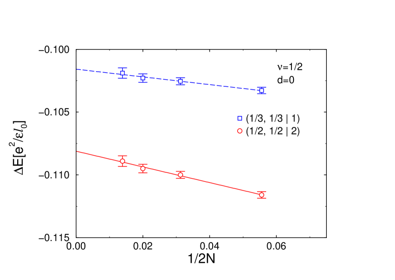
FIG. 1.: The energies of the bilayer states $(1/3,1/3|1)$ and $(1/2,1/2|2)$ at $\nu=1/2$ as a function of $1/2N$, where $2N$ is the total number of particles. The energies are measured relative to the state $(1/4,1/4|0)$, with $\Delta E\equiv E_{(\overline{\nu},\overline{\nu}|m)}-E_{(1/4,1/4|0)}$. The layer thickness and the layer separation are taken to be zero in this plot. In this and in subsequent figures the energies are given in units of $e^{2}/\epsilon l_{0}$, where $l_{0}=\sqrt{\hbar c/eB}$ is the magnetic length and $\epsilon$ is the dielectric constant of the background material.

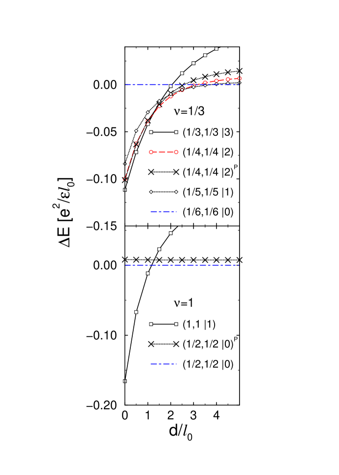
FIG. 2.: The thermodynamic energies of various bilayer composite-fermion states at $\nu=1/3$ and 1, measured relative to the energy of the uncorrelated state $(\nu/2,\nu/2|0)$ as a function of layer separation. Each layer is taken to be strictly two-dimensional in this plot. The various states $(\overline{\nu},\overline{\nu}|m)$ are explained in the text.

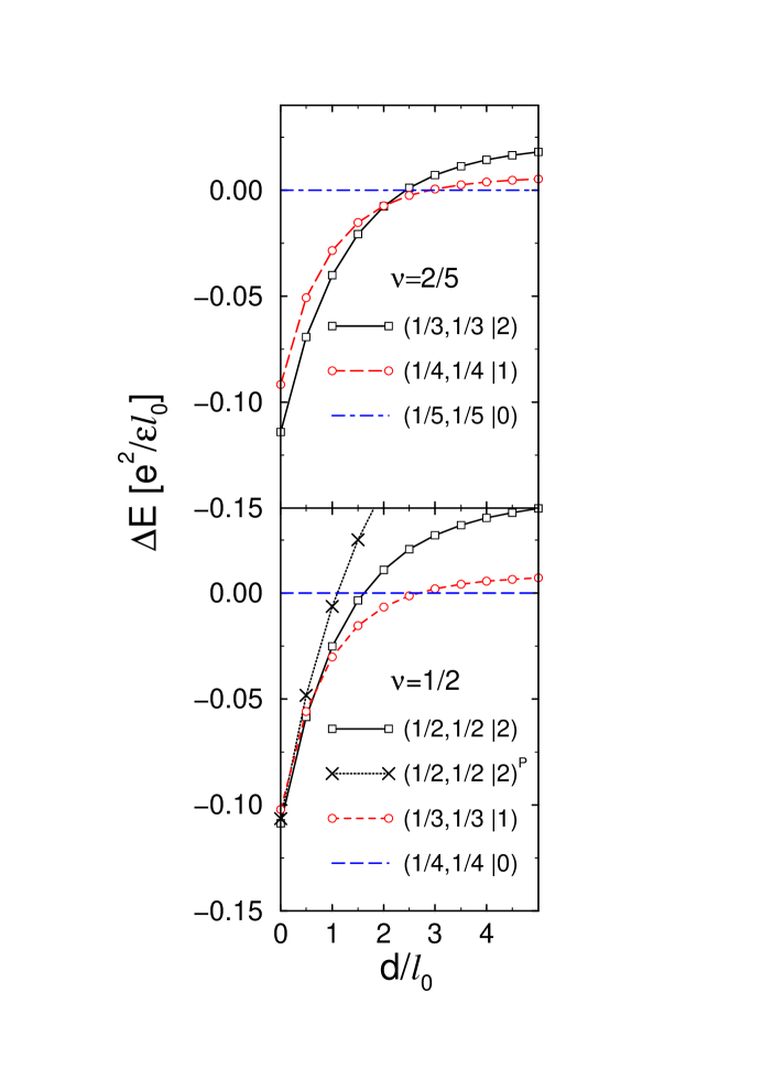
FIG. 3.: The same as Fig. 2 for fillings $\nu=2/5$ and $1/2$.

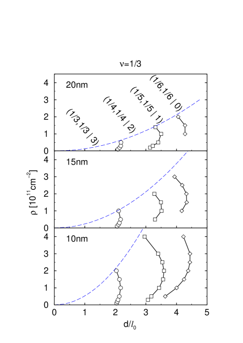
FIG. 4.: The phase diagram of bilayer CF states at $\nu=1/3$ in the $\rho-d$ plane, where $\rho$ is the total electron density and $d$ is the distance between the two layers (measured from center to center). The phase diagram is given for three quantum well widths, 10nm, 15nm, and 20nm. The dashed line shows the minimum distance between the layers, which is equal to the width of the individual single quantum well layer.

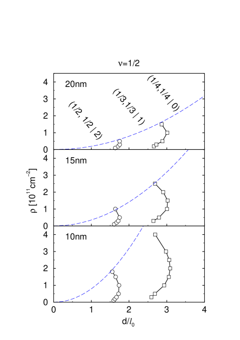
FIG. 5.: The phase diagram of bilayer CF states at $\nu=1/2$ in the $\rho-d$ plane.

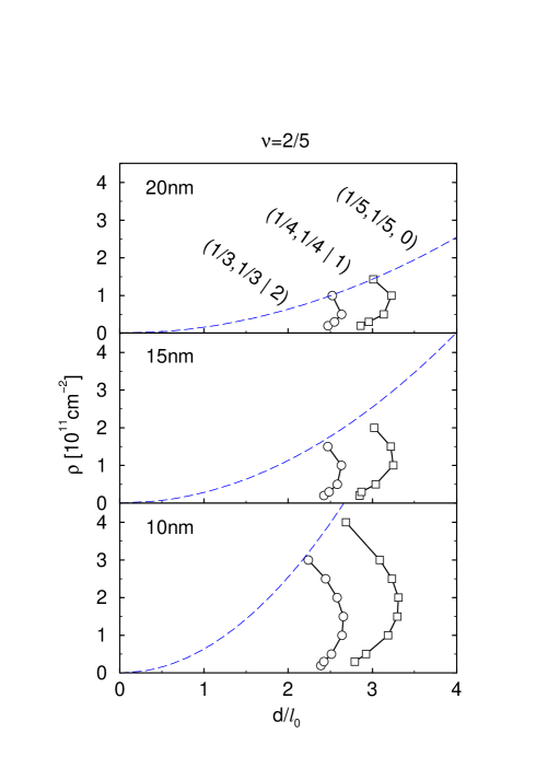
FIG. 6.: The phase diagram of bilayer CF states at $\nu=2/5$ in the $\rho-d$ plane.

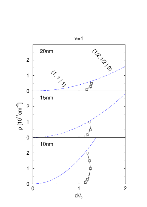
FIG. 7.: The phase diagram of bilayer CF states at $\nu=1$ in the $\rho-d$ plane.

REFERENCES

- [1] B.I. Halperin, Helv. Phys. Acta 56, 75 (1983).
- [2] R.B. Laughlin, Phys. Rev. Lett. 50, 1395 (1983).
- [3] Y.W. Suen et al., Phys. Rev. Lett. 68, 1379 (1992).
- [4] J.P. Eisenstein et al., Phys. Rev. Lett. 68, 1383 (1992).
- [5] S. He, S. Das Sarma, and X.C. Xie, Phys. Rev. B 47, 4394 (1993).
- [6] S.Q. Murphy et al., Phys. Rev. Lett. 72, 728 (1994); T.S. Lay et al., Phys. Rev. B 50, 17725 (1994).
- [7] For experimental and theoretical reviews of multicomponent FQHE, see the chapters by J.P. Eisenstein, and S.M. Girvin and A.H. MacDonald in Quantum Hall Effects, eds. S. Das Sarma and A. Pinczuk (Wiley, New York, 1997).
- [8] I. B. Spielman, J. P. Eisenstein, L. N. Pfeiffer, and K. W. West, cond-mat/0002387 (2000).
- [9] X.G. Wen and Z. Zee, Phys. Rev. B 47, 2265 (1993); Z.F. Ezawa and A. Iwazaki, Phys. Rev. B 48, 15189 (1993).
- [10] J.K. Jain, Phys. Rev. Lett. 63 199 (1989); Phys. Rev. B 41, 7653 (1990); Physics Today 53(4), 39 (2000).
- [11] Note that negative values of are also allowed, with . These correspond to reverse flux attachment, in which the effective magnetic field for composite fermions points in a direction opposite to the external magnetic field.
- [12] V. Kalmeyer and S.C. Zhang, Phys. Rev. B 46, 9889 (1992).
- [13] B.I. Halperin, P.A. Lee, and N. Read, Phys. Rev. B 47, 7312 (1993).
- [14] V.J. Goldman et al., Phys Rev. Lett. 72, 2065-2068 (1994); W. Kang et al., Phys. Rev. Lett. 71, 3850-3853 (1993); R.L. Willett et al., Phys Rev. Lett. 71, 3846-3849 (1993); J.H. Smet et al., Phys. Rev. Lett 77, 2272 (1996); J.H. Smet et al., Phys. Rev. B 56, 3606 (1997).
- [15] X.G. Wu, G. Dev, and J.K. Jain, Phys. Rev. Lett. 71, 153 (1993).
- [16] K. Park et al., Phys. Rev. B 58, R10167 (1998); K. Park and J.K. Jain, Phys. Rev. Lett. 80, 4237 (1998); Phys. Rev. Lett. 83, 5543 (1999); Phys. Rev. B, in press.
- [17] R. Shankar, cond-mat/0009361; G. Murthy, cond-mat/0008259.
- [18] S.S. Mandal and V. Ravishankar, Phys. Rev. B. 54, 8688 (1996).
- [19] R.R. Du, A.S. Yeh, H.L. Stormer, D.C. Tsui, L.N. Pfeiffer, and K.W. West, Phys. Rev. Lett. 75, 3926 (1995); I.V. Kukushkin, K. v. Klitzing, and K. Eberl, Phys. Rev. Lett. 82, 3665 (1999); S. Melinte, N. Freytag, M. Horvatić, C. Berthier, L.P. Lévy, V. Bayot, and M. Shayegan, Phys. Rev. Lett. 84, 354 (2000); A.E. Dementyev, N.N. Kuzma, P. Khandelwal, S.E. Barrett, L.N. Pfeiffer, and K.W. West, Phys. Rev. Lett. 83 5074 (1999); D.R. Leadley, R.J. Nicholas, D.K. Maude, A.N. Utjuzh, J.C. Portal, J.J. Harris, and C.T. Foxon, Phys. Rev. Lett. 79, 4246 (1997).
- [20] G. Murthy, Phys. Rev. Lett. 84, 350 (2000).
- [21] A. Lopez and E. Fradkin, Phys. Rev. B 51, 4347 (1995); R. Rajaraman, Phys. Rev. B 56, 6788 (1997); T.L. Ho, Phys. Rev. Lett. 75, 1186 (1995); Z.F. Ezawa and A. Iwazaki, Phys. Rev. B 47, 7295 (1993); S. Das Sarma and E. Demler, cond-mat/0009372.
- [22] T. Chakraborty and P. Pietilainen, Phys. Rev. Lett. 59, 2784 (1987).
- [23] D. Yoshioka, A.H. MacDonald, and S.M. Girvin, Phys. Rev. B 39, 1932 (1989).
- [24] S. He, X.C. Xie, S. Das Sarma, and F.C. Zhang, Phys. Rev. B 43, 9339 (1991).
- [25] A.H. MacDonald, Surface Science 229, 1 (1990).
- [26] T.T. Wu and C.N. Yang, Nucl. Phys. B 107, 365 (1976); T.T. Wu and C.N. Yang, Phys. Rev. D 16, 1018 (1977).
- [27] F.D.M. Haldane, Phys. Rev. Lett. 51, 605 (1983).
- [28] A. Lopez and E. Fradkin, Phys. Rev. B 44, 5246 (1991).
- [29] R. Shankar and G. Murthy, Phys. Rev. Lett. 79, 4437 (1997).
- [30] J.K. Jain and R.K. Kamilla, Int. J. Mod. Phys. B 11, 2621 (1997); Phys. Rev. B 55, R4895 (1997).
- [31] K. Park, N. Meskini, and J.K. Jain, J. Phys.: Condens. Matter 11, 7283 (1999).
- [32] H.C. Manoharan, Y.W. Suen, M.B. Santos, and M. Shayegan, Phys. Rev. Lett. 77, 1813 (1996).
- [33] J. Schliemann, S.M. Girvin, and A.H. MacDonald, cond-mat/0006309 (2000).
- [34] S.Q. Murphy et al., Phys. Rev. Lett. 72, 728 (1994).
- [35] R.J. Hyndman et al., Surface Science 361/362, 117 (1996).
- [36] A.R. Hamilton et al., Physica B 249-251, 819 (1998).
- [37] Y. W. Suen, H. C. Manoharan, X. Ying, M. B. Santos, and M. Shayegan, Phys. Rev. Lett 72, 3405 (1994).
- [38] G. Moore and N. Read, Nucl. Phys. B 360, 362 (1991).
- [39] M. Grieter, X.G. Wen, and F. Wilczek, Phys. Rev. Lett. 66, 3205 (1991); R. Morf et al., ibid. 80, 1505 (1998); E.H. Rezayi and F.D.M. Haldane, ibid. 84, 4685 (2000); V.W. Scarola, K. Park, and J.K. Jain, Nature 406, 863 (2000).