Abstract

We present a one dimensional model for the development of corrugations in roads subjected to compressive forces from a flux of cars. The cars are modeled as damped harmonic oscillators translating with constant horizontal velocity across the surface, and the road surface is subject to diffusive relaxation. We derive dimensionless coupled equations of motion for the positions of the cars and the road surface $H(x,t)$, which contain two phenomenological variables: an effective diffusion constant $\Delta(H)$ that characterizes the relaxation of the road surface, and a function $a(H)$ that characterizes the plasticity or erodibility of the road bed. Linear stability analysis shows that corrugations grow if the speed of the cars exceeds a critical value, which decreases if the flux of cars is increased. Modifying the model to enforce the simple fact that the normal force exerted by the road can never be negative seems to lead to restabilized, quasi-steady road shapes, in which the corrugation amplitude and phase velocity remain fixed.

1 Introduction

It is commonly observed that under the influence of a flow of traffic, dirt roads develop regular corrugations of longitudinal “pitch,” or wavelength, between 0.5 and 1 m, and amplitude up to 50 mm [1]. At first glance such an instability of the road surface might seem counterintuitive, as one might guess that a flow of traffic would exert downward forces on the surface which tend to smooth and compact the road bed, thereby suppressing pattern development rather than promoting it. Yet irregular, rough roads do not in fact heal themselves, but instead become progressively rougher and more corrugated under a flow of cars. Similar phenomena also occur, though sometimes on different length and time scales, on paved roads, on railroad rails [2], and on the rollers used to calendar paper [3]. The purpose of this paper is to investigate this phenomenon using a simple, tractable physical model.

An early attempt at explaining road corrugation is due to Relton [4], who proposed that the underlying instability mechanism is a “relaxation oscillation,” caused essentially by stick-slip dynamics. According to this view, a moving wheel pushes grains ahead of it. The grains pile up in front of the wheel and form a heap. When the heap grows large enough, the wheel sticks momentarily, and then slips, running over the heap and leaving it behind as a ridge. For a given uniform speed, this stick-slip process will be fairly periodic, and so will generate equidistant ridges.

A different picture was provided by Mather [2], who argued that the origin of the road instability is the bouncing motion of the wheel, caused by random irregularities on the ground. When the bouncing occurs, the car is projected upward along a certain angle and is airborne for a brief time. When it then strikes the ground, the car creates a crater and the motion then repeats itself. According to this picture, it is not the piling up of grains ahead of the vehicle that is responsible for the instability, but the impact stress of the vehicle on the ground. The wavelength of the resulting corrugations will be determined by the competition between the typical distance the car flies over the ground and the size of the crater generated by the impact stress, which should in turn depend on the hardness of the ground and the relaxation time of the ejected grains. Mather’s picture is similar to other surface instabilities involving granular materials, in particular the ripple patterns in wind blown sand [5, 6, 7, 8], where ejected grains are carried away by the wind and land in a place far from the ejection point. In such a nonlocal model, what sets the wavelength of the ripple is the ratio of the flux of the grains to the appropriately scaled saltation length, i.e., the distance that an ejected grain is carried by the wind.

The model we present in this paper builds on Mather’s picture, but we ignore any nonlocal transport of grains along the road, and we assume that the cars, and more specifically their wheels, generally do not lose contact with the road. Instead, we model the cars simply as masses attached to damped springs. We assume that the downward contact forces exerted on the road by the wheels causes a permanent downward deflection of the road surface, by either erosion or plastic deformation. In either case we model the effect of the contact force on the road as a simple proportionality between the deformation at any point on the road and the force exerted on that point, with a phenomenological “softness” parameter as the proportionality constant. We also include a diffusive relaxation that tends to smooth the road surface, which may come about, for instance, as a result of rain. We find that the diffusive relaxation is a stabilizing effect, as one would expect, but that its presence or absence generally has no qualitative effect on the corrugation phenomena. What is important, however, is the phenomenon of hardening. We expect that the softness parameter, and also the diffusion coefficient if it is present, will decrease as the road compacts, so that the road becomes less susceptible to the passage of more cars once the first several have compacted it and perhaps produced corrugations. This turns out to be a stabilizing effect, narrowing the parameter range in which corrugations occur.

Since we are modeling the cars, which in reality are complicated mechanical systems, by simple damped harmonic oscillators, the question quickly arises as to what the appropriate natural frequency might be. Given the observed pitch of road corrugations of 0.5 to 1 m, and the presumed speeds in the range of, say, 10 to 25 m/s of the cars that produce them, we expect that the important oscillation modes must have natural frequencies of about 0.02 to 0.1 s. This is one or two orders of magnitude shorter than the frequency of the car body bouncing on its suspension, so that is unlikely to be the relevant oscillation; indeed drivers normally adjust to the roughness of the road they are on and slow down to avoid such bouncing. This suggests that the relevant mode may be that of the wheel attached to the suspension. Alternatively, the important oscillation may be an elastic deformation of the wheel itself [9]. This could account for an observed difference in the pitch of corrugations produced by hard and soft tires [1].

2 Model

Imagine a flux of cars traveling with some average horizontal velocity $v_{x}$ along a road surface whose height above some arbitrary zero level is given as a function of time $t$ and position $x$ along the road by $H(x,t)$; see Fig. 1. The cars are supported on springs, such that the natural angular frequency of vertical oscillation of the cars is $\omega_{0}$. Further, we assume that the springs are damped with damping constant $b$. Let $Z(x,t)$ be the height of a moving car, relative to a zero level chosen such that $H(x,t)-Z(x,t)$ is the amount by which the springs are compressed. In a frame of reference moving horizontally with the car, the vertical component of the car’s equation of motion comes simply from Newton’s second law,

$$M\frac{d^{2}}{dt^{2}}Z(x,t)+b\frac{d}{dt}[Z(x,t)-H(x,t)]=$$

$$M\omega_{0}^{2}[H(x,t)-Z(x,t)].$$ (1)

Figure 1: A schematic picture of the corrugation of roads. The road surface is subjected to a flux of cars with horizontal speed $v_{x}$, and the cars are modeled as damped harmonic oscillators with mass $M$, spring constant $M\omega_{0}^{2}$, and damping coefficient $b$. The heights of the cars and the surface are $Z(x,t)+\zeta$ and $H(x,t)$ respectively, where $\zeta$ is the equilibrium length of the spring.

The time derivatives here are total derivatives; that is, the relevant value of $x$ is time-dependent, since this equation follows the vertical motion of a single car. We may convert this into an equation for the height of the car at a fixed $x$ by replacing the total time derivative $d/dt$ with $\partial/\partial t+v_{x}(\partial/\partial x)$. Thus in a reference frame that is fixed to the road bed, the vertical equation of motion is

$$M\left(\frac{\partial}{\partial t}+v_{x}\frac{\partial}{\partial x}\right)^{2}Z+b\left(\frac{\partial}{\partial t}+v_{x}\frac{\partial}{\partial x}\right)(Z-H)$$

$$+M\omega_{0}^{2}(Z-H)=0.$$ (2)

Note that we have neglected any possible variation in the horizontal velocity $v_{x}$ of the cars.

We must now write an evolution equation for the height $H(x,t)$ of the road surface. We assume first that the road surface sinks at a rate which is proportional to the downward force on the road. This may be due to compaction of the road bed under the surface or to ejection of loose grains at the surface as a car passes; in either case we expect that the proportionality constant between the downward force on the road and its rate of sinking will decrease as the road sinks. That is, the road should harden as more and more cars pass over it. In addition, we assume that there is a “diffusive” relaxation process which tends to even out any roughness in the road surface. This can result from the action of wind or rain, and may also contain a contribution from the passage of the cars, as the loosely connected grains at the surface are fluidized by the flow of cars. Again, we expect the effective diffusion coefficient to decrease as cars pass and the road hardens. With these assumptions, the equation of motion for the road height reads

$$\frac{\partial H}{\partial t}=D(H)\frac{\partial^{2}H}{\partial x^{2}}-a(H)\left[Mg+M\omega_{0}^{2}(H-Z)\right],$$ (3)

where $Mg$ is the weight of a car. We are neglecting the geometrical distinction between $\partial H/\partial t$ and the rate of motion of the road surface normal to itself, and also the fact that the compressive force is not really vertical when $H$ is not constant. These are satisfactory approximations provided the vertical scale of the surface corrugations is much smaller than the horizontal scale. However, these effects should be included in any model of road corrugation which is nonlinear in the amplitude of the corrugation.

The proportionality factor $a(H)$ above represents the softness of the road, that is, its responsiveness to compressing forces. It should include the flux of cars as a multiplicative factor, as the rate of road sinking should also depend on the density of the traffic it sustains. The compression term should be replaced by zero whenever the quantity in brackets is negative, since that represents the situation in which the cars are airborne, so that the compressive force on the road would really be zero rather than negative. Requiring that the road harden as it compacts means that $a$ (and probably also $D$) should decrease as $H$ decreases, so we want $a(H)$ to be positive and an increasing function of $H$. A physically acceptable form of $a(H)$ is shown in Fig. 2.

Figure 2: A physically plausible form for the softness or compactivity function $a(H)$. We require $a$ to be an increasing function of $H$ which either approaches zero for $H\to-\infty$ or vanishes for $H$ below some fixed, finite limit.

Before proceeding, we first nondimensionalize the equations of motion for $Z$ and $H$. We choose the time scale to be $1/\omega_{0}$, the horizontal length scale to be $v_{x}/\omega_{0}$, and the vertical length scale to be $g/\omega_{0}^{2}$. The equation of motion for the cars then becomes

$$\left(\frac{\partial}{\partial t}+\frac{\partial}{\partial x}\right)^{2}Z+2\Gamma\left(\frac{\partial}{\partial t}+\frac{\partial}{\partial x}\right)(Z-H)+Z-H=0,$$ (4)

and the equation for the road surface is

$$\frac{\partial H}{\partial t}=\Delta(H)\frac{\partial^{2}H}{\partial x^{2}}-\alpha(H)(1+H-Z),$$ (5)

where the new dimensionless parameters are given by

$$\Gamma=b/2M\omega_{0},\qquad\Delta(H)=(\omega_{0}/v_{x}^{2})\,D(H),$$

$$\qquad\alpha(H)=M\,\omega_{0}\,a(H).$$ (6)

The parameter $\Gamma$ is a property of the cars alone; the cars’ springs are underdamped for $\Gamma<1$. Since the instability is controlled by the interplay of essentially two mechanisms, ejection of grains from the surface or compaction of the road by the flux of cars and subsequent relaxation of the road surface due to diffusion, $\Gamma$ and $\Delta$ will control the dynamics of the surface. As we will see, the hardening of the road also plays an important role in the development of the instability.

3 Linear Stability Analysis

We may solve the system of partial differential equations (4) and (5) numerically, and we will discuss this below, but useful information regarding the behavior of the system may also be extracted from an approximate linear stability analysis. The first step in the analysis is to recognize that as time increases, the spatially averaged values of $Z(x,t)$ and $H(x,t)$ will tend to decrease, reflecting the gradual settling of the road bed. We denote this spatially averaged, i.e. spatially independent, quiescent solution by $H_{0}(t)$ and $Z_{0}(t)$. Substituting this solution into the equations of motion, we find that it satisfies

$$\ddot{Z}_{0}+2\Gamma(\dot{Z}_{0}-\dot{H}_{0})+Z_{0}-H_{0}=0.$$ (7)

and

$$\dot{H}_{0}=-\alpha(H_{0})(1+H_{0}-Z_{0}),$$ (8)

The full solution may now be written as

$$H(x,t)=H_{0}(t)+h(x,t),\qquad Z(x,t)=Z_{0}(t)+z(x,t),$$ (9)

in which the functions $h(x,t)$ and $z(x,t)$ will carry information about pattern development. Substituting these forms of $H(x,t)$ and $Z(x,t)$ into (4) and (5), using (7) and (8) for the time evolution of $Z_{0}$ and $H_{0}$, and expanding to first order in $h$ and $z$, we obtain the following linearized equations of motion:

$$\left(\frac{\partial}{\partial t}+\frac{\partial}{\partial x}\right)^{2}z+2\Gamma\left(\frac{\partial}{\partial t}+\frac{\partial}{\partial x}\right)(z-h)+z-h=0,$$ (10)

$$\frac{\partial h}{\partial t}=\Delta\frac{\partial^{2}h}{\partial x^{2}}-\alpha(h-z)-\beta h,$$ (11)

where $\alpha$ and $\Delta$ are evaluated at $H=H_{0}$, and $\beta$ is given by

$$\beta=(1+H_{0}-Z_{0})\,\alpha^{\prime}(H_{0})=-\frac{d\hbox{ln}\alpha(H_{0})}{dt}.$$ (12)

The last equality here follows from (8). Note that $\beta$ should be positive, since we expect that $\alpha$ will increase with $H$ and decrease with time.

If $\alpha$ and $\Delta$ are nontrivial functions of $H$, then it is not simple to solve the linearized equations (10) and (11), because the coefficients in the latter equation are functions of time. However, we may perform an approximate stability analysis by regarding $\alpha$, $\beta$, and $\Delta$ as constants, at least for short time intervals, and calculating the linear growth rates that obtain when those parameters have their current values. Thus we will determine time dependent growth rates and phase velocities, provided we can ascertain the time dependent forms of $\alpha$ and $\Delta$.

We proceed by assuming both $h$ and $z$ to be proportional to $\exp(ikx+\sigma t)$, where the linear growth rate $\sigma$ is in general complex. As usual, $Re[\sigma]$ is the exponential growth or decay rate of the amplitude of a perturbation with wave number $k$, and $Im[\sigma]$ is related to the phase velocity $c$ of that mode through $c=-Im[\sigma]/k$. This substitution yields

$$[(\sigma+ik)^{2}+2\Gamma(\sigma+ik)+1]z=[1+2\Gamma(\sigma+ik)]\,h$$ (13)

and

$$\sigma h=-\Delta k^{2}h-\alpha(h-z)-\beta h.$$ (14)

Eliminating $h$ between these equations gives the stability relation

$$[(\sigma+ik)^{2}+2\Gamma(\sigma+ik)+1]\,(\beta+\sigma+\Delta k^{2})+\alpha\,(\sigma+ik)^{2}=0,$$ (15)

from which we can find the growth rates and phase velocities of spatially sinusoidal perturbations in terms of their wave numbers.

It is possible to determine the stability boundary for the model, at least parametrically, from (15). That is, we could determine the locus in parameter space on which the real part of the linear growth rate $\sigma$, as a function of $k$, has a global maximum at height $Re[\sigma]=0$. However, it is much more instructive to simplify the already approximate problem further by taking $\alpha$ and $\Delta$ to be small, as we expect to be the case once the road has had a chance to harden sufficiently. To set the stage for this calculation, imagine setting $\alpha=0$ in (15). The cubic equation for $\sigma$ would then factor. Two of the solutions would always have negative real parts, since $\sigma+ik$ for these two solutions would be a root of a quadratic with positive coefficients; these represent decaying perturbation modes. The third would be $\sigma=-\beta-\Delta k^{2}$, so this mode too would always be stable unless $\beta$ is also small, on the same order as $\alpha$ or smaller. Note that small $\alpha$ does not necessarily imply that $\beta$ must be small, because $\beta$ is the logarithmic derivative of $\alpha$.

Since we are interested in finding parameter ranges for which corrugations grow, we now focus on the case where $\alpha$, $\beta$, and $\Delta$ are all small. As we just saw, only one of the three solutions for $\sigma$ can possibly be positive; to leading order in the small parameters it is given by

$$\sigma=-\beta-\Delta k^{2}+\alpha k^{2}\frac{(1-k^{2})-2i\Gamma k}{(1-k^{2})^{2}+4\Gamma^{2}k^{2}}.$$ (16)

Figure 3: The approximate stability diagram in the $(\beta/\alpha)$–$(\Delta/\alpha)$ plane, obtained from (16), for values of the damping parameter $\Gamma$, ranging from 0.3 (top) to 0.9 (bottom) in steps of 0.1. All stability boundaries For $\Gamma\geq 0.5$ pass through the point (0,1). The flat road surface is stable above and to the right of the boundary curve for the appropriate $\Gamma$ value.

We may locate an approximate stability boundary by seeking combinations of parameters for which the real part of this $\sigma$ has a maximum, as a function of wave number $k$, at $Re[\sigma]=0$. Thus we solve the equations $Re[\sigma]=0$ and $d(Re[\sigma])/dk=0$ to obtain the critical values of $\beta/\alpha$ and $\Delta/\alpha$ parametrically in terms of $k$. The results are shown for several values of the damping parameter $\Gamma$ in Fig. 3. As is clear from (16), both $\beta$ and $\Delta$ represent stabilizing effects, so for a given $\Gamma$, the flat road surface is stable above and to the right of the stability boundary curve for that $\Gamma$. The stability boundaries move down and left as $\Gamma$ is increased, so damping of the car’s springs also tends to stabilize the flat road surface. One can show explicitly that the stability boundary reaches $\Delta=0$ at $\beta/\alpha=[4\Gamma(1+\Gamma)]^{-1}$, and it reaches $\beta=0$ at $\Delta/\alpha=[4\Gamma(1-\Gamma)]^{-1}$ for $\Gamma<1/2$ or $\Delta/\alpha=1$ for $\Gamma>1/2$. Moreover, for small $\Gamma$ – that is, when the oscillations of the car springs are very slightly damped – the stability boundary is given approximately by the line $\Delta+\beta=\alpha/4\Gamma$.

To find the wave numbers of the most important perturbations, we first note from (16) that the parameter $\beta$ only enters the expression for the growth rate additively. As a result, the wave number $k_{max}$ at which the real part of $\sigma$ has its maximum is independent of $\beta$; it is given explicitly by

$$\frac{\Delta}{\alpha}=\frac{(1-k_{max}^{2})^{2}-4\Gamma^{2}k_{max}^{4}}{[(1-k_{max}^{2})^{2}+4\Gamma^{2}k_{max}^{2}]^{2}}.$$ (17)

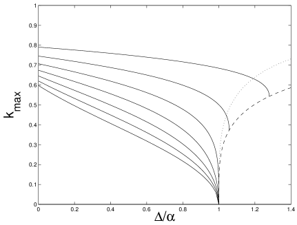
Figure 4: The wave number of the perturbation whose linear growth rate is maximal, plotted as a function of $\Delta/\alpha$ for various values of the damping parameter $\Gamma$ ranging from 0.3 (top) to 0.9 (bottom) in steps of 0.1. The dashed curve marks where the local maximum in $Re[\sigma(k)]$ merges with a local minimum and vanishes. Between it and the dotted curve, $Re[\sigma]$ has a local maximum at the indicated $k$, but the global maximum is at $k=0$.

Fig. 4 shows $k_{max}$ as a function of $\Delta/\alpha$ for several values of the damping constant $\Gamma$. (Below and to the right of the dotted curve, the maximum growth rate is negative for any positive value of $\beta$, so the flat road surface can only be unstable when $\Delta/alpha$ is to the left of the dotted curve.) We see that the wave number of the most rapidly growing mode decreases with increasing damping $\Gamma$; it also decreases with increasing $\Delta/\alpha$, although the dependence on $\Delta/\alpha$ is weak when $\Gamma$ is small. In fact, for small $\Gamma$ we always have $k_{max}=1-\Gamma+O(\Gamma^{2})$. In no case do we find $k_{max}$ to be above 1. Recall that $k$ is the wave number of the perturbation in units of $\omega_{0}/v_{x}$. Thus the fact that $k_{max}$ is always less than 1 means that the wavelength of the most rapidly growing perturbation is always greater than $(2\pi/\omega_{0})\,v_{x}$, the distance a car travels in one period of its natural oscillation.

From the imaginary part of $\sigma$ we obtain the drift velocity $c$ of a perturbation of wave number $k$ (in units of $v_{x}$),

$$c=-Im[\sigma]/k=\frac{2\alpha\Gamma k^{2}}{(1-k^{2})^{2}+4\Gamma^{2}k^{2}}.$$ (18)

Note the factor $\alpha$: since $\alpha$ is small, the drift velocity is small compared to $v_{x}$, the speed of the cars. Also, since $\alpha$ contains a factor of the number of cars passing per unit time, the drift is actually a fixed distance per passing car, rather than per unit time. The drift velocity is positive, so that corrugations are pushed in the direction that traffic is moving as they develop. It reaches its maximum value of $\alpha/2\Gamma$ at $k=1$.

4 Numerical Results

Since the linear stability analysis of the preceding section is only approximate, we have found it useful to check its results by carrying out numerical simulations of the full model given by Eqns. (4) and (5). We choose a wave number $k$, choose a sinusoidal form for the initial $H(x)$ and $Z(x)$ with small amplitudes, and then integrate the equations on an interval of length $2\pi/k$ with periodic boundary conditions. We the monitor the amplitudes and phase velocities of $H$ and $Z$ as time passes. The logarithmic derivative of the amplitudes with respect to time gives the instantaneous exponential growth rate $\sigma(t)$.

For the non-constant $\alpha$ cases we use the simple ansatz

$$\alpha(H)=\alpha_{0}\,\exp(\epsilon H),\qquad\epsilon>0,$$ (19)

which has the qualitative form shown in Fig. 2 and is mathematically tractable. The parameter $\epsilon$ controls the rate at which the soil hardens. We may solve for the time evolution of the quiescent road level $H_{0}$ provided $\alpha$ is small, for then $Z_{0}$ varies on a much shorter time scale than $H_{0}$, and so $Z_{0}$ should always remain near $H_{0}$. Then (8) reduces to

$$\dot{H}_{0}=-\alpha(H_{0})=-\alpha_{0}\,\exp(\epsilon H_{0}).$$ (20)

This can be integrated immediately to yield $\exp(-\epsilon H_{0})=\epsilon\alpha_{0}(t+t_{0})$, where $t_{0}$ is a constant of integration. From this we get

$$\alpha=\frac{1}{\epsilon(t+t_{0})},$$ (21)

and from the definition (12) of $\beta$ we then get

$$\beta=\frac{1}{t+t_{0}}=\epsilon\,\alpha,$$ (22)

so that the combination $\beta/\alpha$ that appears in the approximate linear stability analysis is just the constant $\epsilon$.

Figs. 5a and 5b show typical numerical and theoretical determinations of the growth rate $Re[\sigma(t)]$ and phase velocity $c(t)=-Im[\sigma(t)]/k$ for $\alpha$ given by (19) above and $\Delta$ constant, for various values of the hardening parameter $\epsilon=\beta/\alpha$. As expected, for a given value of $k$ the agreement is quite strong; this continues to hold over a range of $\alpha_{0}$ and $\epsilon$.

Figure 5: (a) Linear growth rate $Re[\sigma]$ and (b) phase velocity $c$ vs. time for single mode solutions in the case $\alpha=\alpha_{0}\exp(\epsilon H)$ with $k=0.90$, $\alpha_{0}=0.004$, $\Gamma=0.1$, $\Delta=0.01$, $\epsilon=0.5$ circle, $0.1$ square, $0.05$ diamond, $0.01$ triangle. Continuous lines are from numerical solution of the full equations, symbols from the approximate linear stability analysis.

It is clear from the the linear stability analysis that if the diffusion parameter $\Delta$ remains finite as $\alpha$ decreases to zero, or more generally if $\alpha/\Delta$ goes to zero as the road compacts, then we will eventually reach a situation in which diffusion dominates the dynamics. From that point on, any corrugation in the road will decay. On the other hand, we certainly expect that as the road compacts and its surface hardens, the hardening should inhibit the lateral transfer of material which we have modeled as diffusion, as well as further compaction of the road. We see, then, that in order to get nontrivial corrugations on the road surface, we must have $\Delta$ decrease at least as rapidly as $\alpha$ as the road compacts.

To investigate the possibility of generating corrugation patterns, we examine the simplest nontrivial case, namely where $\Delta$ and $\alpha$ have the same $H$-dependence, $\Delta(H)=\Delta_{0}\exp(\epsilon H)$ and $\alpha(H)=\alpha_{0}\exp(\epsilon H)$. As above, this ansatz leads to $\beta/\alpha$ being constant – specifically, equal to $\epsilon$ – and all three parameters $\alpha$, $\beta$, and $\Delta$ decreasing as $t^{-1}$ at long times $t$. From (16) we then see that the linear growth rate $\sigma$ is also proportional to $t^{-1}$ for large $t$. Figures 6a and 6b show this slow decrease of the real and imaginary parts of $\sigma(t)$ for a few single mode solutions, arrived at by numerical solution and stability analysis.

Figure 6: (a) Linear growth rate $Re[\sigma]$ and (b) phase velocity $c$ vs. time for single mode solutions with $\alpha=\alpha_{0}\exp(\epsilon H)$ and $\Delta=\Delta_{0}\exp(\epsilon H)$. Parameter values are $k=0.85$, $\alpha_{0}=0.006$, $\Delta_{0}=0.01$, $\Gamma=0.1$, $\epsilon=0.5$ circle, $0.1$ square, $0.05$ diamond, $0.01$ triangle. Continuous lines are from numerical solution of the full equations, symbols from the approximate linear stability analysis.

Since $\sigma$ is the logarithmic time derivative of the amplitude of a perturbation, we see that the amplitude itself grows or decays algebraically in the long-time limit:

$$\frac{d\ln A}{dt}=\sigma=\frac{\sigma_{0}}{t+t_{0}}\qquad\rightarrow\qquad A\propto(t+t_{0})^{\sigma_{0}}.$$ (23)

Thus the growth rate of the corrugation amplitude becomes small at long times in this model, but the corrugation does not reach a true steady state.

Figure 7: Quasi-steady state amplitude vs. $k$ in the case of constant $\alpha$, but setting $\alpha=0$ when $1+H-Z<0$. Parameter values are $\Gamma=0.10$, $\Delta=0.01$, $\alpha=0.0040$ circle, $0.0045$ square, $0.0050$ diamond, $0.0055$ triangle, $0.0060$ plus.

Figure 8: (a) Quasi-steady state phase velocity (symbols) $c$ vs. $k$ in the cases described in Fig. 7. The upper and lower solid curves mark where $c(k)$ would lie if the force were not removed when $1+H-Z<0$, for $\alpha=0.0055$ and 0.0040 respectively. (b) The finer structure in the data presented in (a) is visible here. We plot $c_{diff}=c(\alpha=0.0060)-c(\alpha)$ vs. $k$. Parameters are $\alpha=0.0055$ circle, $0.0050$ square, $0.0045$ diamond, $0.0040$ triangle.

It is clearly of interest to determine whether restabilized steady states exist. However, such states would depend on a host of nonlinear effects which are omitted in the model embodied in Eqns. (4) and (5). While we do not believe our model as presented is capable of predicting steady states, we have observed a remarkable feature in some of our numerical calculations. We have investigated cases in which $\alpha$ and $\Delta$ are constants. These cases neglect the hardening effect which, as we saw above, tends to stabilize the flat road surface; the parameter $\beta$ vanishes. The linear stability analysis is then exact, and we expect to find purely exponential growth or decay of $h$ and $z$. Our numerical calculations show that modes that are stable according to the linear stability analysis do indeed decay in amplitude. Modes which are linearly unstable grow until their amplitudes are so large that we have $1+H(x,t)-Z(x,t)<0$ for part of the cycle. When this happens, (5) suggests – unphysically – that the compression of the road is negative. What is happening here is that the cars are losing contact with the road. To avoid having the road surface spontaneously rise when an airborne car passes over it, we set $\alpha=0$ whenever we are in this situation.

Such a detachment in fact does occur in real situations, and has been termed “bouncing” [9]. In a laboratory experiment involving two rotating disks that are in contact with each other under static compression, the two disks lose contact and bounce against each other when the amplitude of the corrugation along the perimeter of the disks exceeds about 1/3 the static compression. In the case of a car moving on a corrugated surface, such bouncing will kick the car into the air, but the car will quickly land in a different place, a mechanism suggested by Mather [2]. Such a bouncing motion should involve a local flux of the cars and a saltation function that relates the landing position to the start-off position, as in the case of wind-blown sand [5, 6, 7]. We note that such a nonlocal behavior would be difficult to account for in the model completely, but our mechanism of setting $\alpha$ locally to zero captures some of its flavor. Our expectations are that the modes that grow large enough to be subject to the local removal of the the force term in (5) will obviously have their growth rates reduced from those predicted by the linear stability analysis in the absence of such a force removal, and that this reduction in growth rate may be sufficient to generate steady states with finite amplitudes. To test this intuition, we numerically solve the system using single cycles of sinusoidal modes $k$, in periodic systems whose lengths are a single wavelength. The initial disturbances are chosen with amplitudes large enough to cause $1+H(x,t)-Z(x,t)$ to be negative on occasion.

Provided a given mode is unstable according to the linear stability analysis, our numerical analysis indicates that it evolves toward a quasi-steady state in which the amplitude and phase velocity $c$ of the road corrugations remain fixed, even while the average height of the road bed continues to sink. Fig. 7 shows the steady state amplitudes of $h$ as a function of $k$ for $\Gamma$, $\Delta$, and$\alpha$ as given in the figure caption. For fixed $k$, the steady state amplitudes increase with increasing $\alpha$. Thus we see for this choice of parameters that softer roads (i.e., larger $\alpha$) support larger disturbances in the steady state than do harder ones. This result is intuitively satisfying, as we expect the ease of deformation of the material to correlate with the amplitude of the disturbance it supports. The phase velocities of the quasi-steady states exhibit particularly interesting behavior. Fig. 8a shows the observed quasi-steady state phase velocities, plotted as symbols, and an “envelope” in the $k-c$ plane. If there were no step function in the term in $\alpha$, the phase velocities would lie in the region bounded by the envelope. The top curve would be the velocity curve for the largest $\alpha$ used (0.0055) and the bottom curve would be the velocity curve for the smallest $\alpha$ used (0.0040). The step function in the compactivity has forced the phase velocities to “collapse” so that they seem to lie along or near a single curve in the $k-c$ plane. Examination of the quasi-steady state velocities on a finer scale, as shown in Fig. 8b, indicates a persistence of the kind of variation of phase velocity with softness we have typically seen (that is, the softer the road, or equivalently the larger $\alpha$ is, the greater the phase velocity, all other things being equal), though this variation exists on a much finer scale in the steady state case than in the case in which the step function is not invoked.

Even though we have identified interesting steady state behavior in the solution of the differential equations in this limiting case of $\alpha$ being constant, we must reiterate that setting $\alpha$ to a constant is certainly unphysical, and that many nonlinear effects have been omitted from our model equations. Moreover, our model does not account carefully for what happens when contact with the road and cars is lost; it merely turns off the coupling between cars and road in the equation of motion for $H(x,t)$, and furthermore assumes the evolution of $Z(x,t)$ remains well described by Eq. (4). Thus we cannot expect that our nonlinear calculations will speak to the behavior of real roads. Nonetheless, we find it remarkable that simply setting $\alpha=0$ when $1+H(x,t)-Z(x,t)$ is negative seems to contain the growth of the unstable modes.

5 Conclusions and Prospects

In this work, we have explored the origin of the corrugation instability of dirt roads subjected to a constant flux of cars. We have presented a simple phenomenological model for the evolution of the road surface and carried out a linear stability analysis to uncover the gross features of the instability. ¿From our approximate stability analysis and its numerical verification, we find that the dynamical processes of diffusion and compression in a road bed are sufficient to generate instabilities that can give rise to pattern formation. Small-amplitude corrugations on the road surface grow when the diffusion parameter $\Delta/\alpha$ and the hardening parameter $\beta/\alpha$ lie below the stability boundary (for the appropriate damping coefficient $\Gamma$ for the cars) shown in Figure 3. From the definitions (6) of $\alpha$ and $\Delta$ in terms of the original, dimensional softness and diffusion coefficients $a(H)$ and $D(H)$, we see that the dimensionless combination $\Delta/\alpha$ is inversely proportional to the square of $v_{x}$, the horizontal speed of the cars across the road. Thus we find that there is a critical car speed above which the flat road surface is unstable. Also, since $a(H)$ is proportional to the flux of cars, there is a critical flux for any given speed, above which the flat road is unstable. Both diffusive relaxation and hardening of the surface are stabilizing effects. The wave number of the most rapidly growing mode is given implicitly in dimensionless terms by (17), which is plotted in Fig. 4.

Our model is clearly schematic; a quantitative theory of road corrugations would need to incorporate a number of effects we left out of our calculations. We have not attempted to account, for instance, for the geometric distinction between $\partial h/\partial t$ and the normal velocity of the road surface as it compacts, nor for the fact that the force exerted by a moving car on a corrugated road surface is not purely vertical. For these reasons alone we have not carried out any nonlinear analysis on our model – the model is explicitly not valid beyond linear order in the amplitude of the incipient corrugation. We have also ignored all details of the physical processes by which the road compacts, so it is not clear how well our phenomenological picture of compaction being proportional to applied vertical force or impulse can describe the dynamics of a real road. Our model for the cars is the simplest possible, neglecting the multiplicity of oscillation modes of real cars and the Hertzian nature of the contact force between the tires and the road. In particular, the fact that real vehicles have two or more pair of tires separated by fixed distances may introduce a new, relevant length scale into the problem. Finally, a quantitative theory would have to incorporate distributions of vehicle sizes, weights, oscillation frequencies, speeds, and the like.

Despite the fact that most nonlinear effects are omitted from our model, we find particularly interesting the numerical result that simply setting the contact force to zero when the equations would make it negative can lead to an apparently steady state. At least this results in a drastic slowing of the dynamics once a certain road configuration has been established. Continuing work will focus on determining the selection mechanism of such “frozen” states, and their response to local perturbations.

References

- [1] J. Stoddart, R. Smith, and R. M. Carson, Transp. En. J. 108, 376 (1982).
- [2] K. B. Mather, Civ. Eng. Public Works Rev. 57, 617, 781 (1962); Scientific American 206(1), 128 (1963).
- [3] J. Papadopoulos, private communication.
- [4] F. E Relton, Roads and Road Constr. 16, 340 (1938).
- [5] R. A. Bagnold, Proc. Roy. Soc. A157, 594 (1936); See also The Physics of Blown Sand and Desert Dunes (Morrow, New York, 1941).
- [6] K. Pye and H. Tsoar, Aeolian Sand and Sand Dunes (Unwin Hyman, London, 1990).
- [7] H. Nishimori and N. Ouchi, Phys. Rev. Lett. 71, 197 (1993).
- [8] D. A. Kurtze, J. A. Both, D. C. Hong, Phys. Rev. E 61, 6750 (2000).
- [9] R. M. Carson and K. L. Johnson, Wear, 17, 59 (1971).