Effect of Surface Roughness on the Universal Thermal Conductance

Abstract

We explain the reduction of the thermal conductance below the predicted universal value observed by Schwab et al. [Nature (London) 404, 974 (2000)] in terms of the scattering of thermal phonons off surface roughness using a scalar model for the elastic waves. Our analysis shows that the thermal conductance depends on two roughness parameters: the roughness amplitude $\delta$ and the correlation length $a$. At sufficiently low temperatures the ratio of the conductance to the universal value decreases quadratically with temperature at a rate proportional to $\delta^{2}a$. Values of $\delta$ equal to $22\%$ and $a$ equal to about $75\%$ of the width of the conduction pathway give a good fit to the data.

I Introduction

Ballistic transport in mesoscopic system has been an active area of study. Following Landauer’s approach to electronic conductance, several groups have derived expressions for the thermal conductance due to ballistic phonon transport in an ideal elastic beam.[1, 2, 3] The formula they derived shows that the only material and geometry dependence of the thermal conductance arises through the long wavelength cutoff frequencies of the elastic waves in the beam. As the temperature $T\rightarrow 0$, the conductance is dominated by the lowest few modes with zero cutoff frequency. The conductance then takes on a universal value $K_{u}$ with the value $N_{0}(\pi^{2}k_{B}^{2}T)/(3h)$ with $N_{0}$ the number of modes with zero cutoff frequency at long wavelengths, which is four for a free standing beam. Based on these theoretical predictions, great efforts have been  made to observe the universal thermal conductance. Recently, Schwab et al.[4] successfully observed the universal thermal conductance in a suspended silicon nitride bridge. Their experiment shows a result consistent with the universal conductance at temperatures below about $0.08$ K. Above about $1$ K the conductance rises above this value, as the modes with nonzero cutoff frequencies become excited and contribute to the heat transport. However in the range $0.1$ K$\sim 0.4\$K the thermal conductance unexpectedly decreases below the universal value.

Motivated by the results of Schwab et al. we theoretically investigate a likely cause of the low-temperature thermal conductance decrease. We suggest that the conductance decrease is caused by scattering due to rough surfaces. Recent advanced crystal growth technology guarantees very few impurities in the material during a substrate growth, thus eliminating the possibility of impurity scattering. On the other hand, chemical etching can produce surface roughness on a scale of tens of nanometers, large enough to cause significant scattering.

In this paper we use a simple scalar model for the elastic waves. We also use a two-dimensional approximation, which is accurate at low enough temperatures that modes with structure across the depth of the beam—the smallest dimension in the experimental geometry—are not excited. We also assume that the important roughness is on the sides of the beam, rather than the top and bottom surfaces, since the horizontal surfaces are MBE grown and have roughness at a scale of a few atomic layers, while the side faces are chemically etched. Kambili et al.[5] have used a similar model in a numerical investigation of the effect of surface roughness on the mode propagation.

In the following section, the details of the two-dimensional ($2$D) scalar model are introduced, and the scattered field calculation using a Green function approach is presented. In Sec. III, the scattering probabilities and transmission coefficients are calculated and the latter is incorporated into the modified Landauer formula for thermal conductance. In Sec. IV, the thermal conductance is evaluated numerically and compared to the experiments of Schwab et al.

II Mode Scattering

A The model

The expression for the thermal conductance $K$ of a suspended mesoscopic beam connecting two thermal reservoirs is[1, 2, 3]

$$K={\frac{\hbar^{2}}{{k_{B}T^{2}}}}\sum_{m}{\frac{1}{{2\pi}}}\int_{\omega_{m}}^{\infty}{\cal T}_{m}(\omega){\frac{\omega^{2}e^{\beta\hbar\omega}}{{(e^{\beta\hbar\omega}-1)^{2}}}}d\omega.$$ (1)

Here the integration is over the frequency $\omega$ of the modes $m$ propagating in the beam and $\omega_{m}$ is the cutoff frequency of the $m$th mode. Also $\beta=1/(k_{B}T)$, $k_{B}$ is the Boltzmann constant, $T$ is the temperature, and $\hbar$ is Planck’s constant. The effect of scattering is introduced through the transmission coefficient ${\cal T}_{m}(\omega)$: for the ideal case with no scattering ${\cal T}_{m}=1$. Thus, the change of the thermal conductivity due to the rough surface is obtained by finding the transmission coefficient.

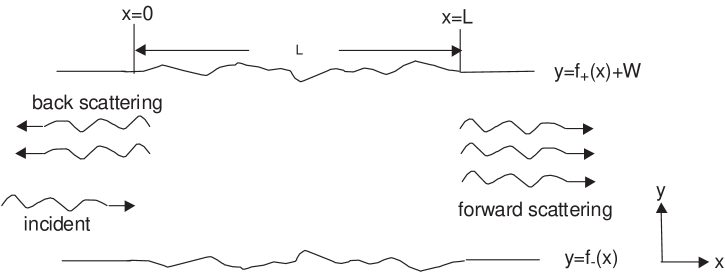
FIG. 1.: $2$D model used for calclation of the scattering of elastic waves by rough surfaces.

As discussed in the introduction, we use a scalar model for the elastic waves, and model a thin geometry at low temperatures so that a two-dimensional calculation is adequate. Thus we consider a $2$D wave-guide-like structure extended in the $x$ direction and bounded at $y=0,W$ in the absence of roughness. The waves satisfy the scalar wave equation, and we assume Neumann boundary conditions at the edges of the wave guide, corresponding to a stress free boundary condition for the elastic waves. Note that Dirichlet boundaries do not support the modes with zero cutoff frequency that are a crucial feature of the elastic problem. We calculate the scattering process by considering an elastic wave propagating in the wave guide in the $+x$ direction with wave vector $k_{0}$ and entering a rough surface region of length $L$ ($0<x<L$) where the rough boundaries are at $y=W+f_{+}(x)$ and $y=f_{-}(x)$ so that the roughness is characterized by the functions $f_{\pm}\left(x\right)$ (see Fig. 1). We assume that the top and the bottom roughness functions are uncorrelated, and that $f_{\pm}\left(x\right)$ is small and is differentiable. The incident wave $\Psi_{\text{in}}$ interacts with the roughness, is scattered into other modes $\Psi_{\text{sc}}$, and leaves the rough region. The total field $\Psi$ is the sum of the incident field and the scattered field

$$\Psi=\Psi_{\text{in}}+\Psi_{\text{sc}}.$$ (2)

Our task is to find an expression for $\Psi_{\text{sc}}$ and hence calculate the transmission coefficients. We do this using a Green function method.

B Green function method

We start with the Helmholtz equation for a scalar wave at frequency $\omega$

$$\nabla^{2}\Psi\left(x,y\right)+K^{2}\Psi\left(x,y\right)=0,$$ (3)

where $\Psi$ is the total field, and $K$ is $\omega/c$ with $c$ the wave speed. Define the Green function as a solution to the point sources

$$\nabla^{2}G\left(x,y;x^{\prime},y^{\prime}\right)+K^{2}G\left(x,y;x^{\prime},y^{\prime}\right)=-\delta\left(x-x^{\prime}\right)\delta(y-y^{\prime})$$ (4)

with $\left(x^{\prime},y^{\prime}\right)$ the source coordinates and $\left(x,y\right)$ the observation coordinates. It is convenient to define $G\left(x,y;x^{\prime}y^{\prime}\right)$ such that it satisfies Neumann boundary conditions at the smoothed boundaries, $y=0,W$

$$\partial G/\partial n|_{y=0,W}=0,$$ (5)

where $\hat{n}$ is the outward-pointing normal to the surface. We then project the physical boundary conditions at the rough surfaces onto the smoothed boundaries to calculate the scattering.

Multiplying Eq. (3) by $G(x,y;x^{\prime},y^{\prime})$ and Eq. (4) by $\Psi(x,y)$ and integrating over a volume bounded by the position of the smoothed surfaces yields the result of Green’s theorem

$$\Psi\left(x,y\right) =\int_{\text{smooth}}dx^{\prime}\frac{\partial\Psi\left(x^{\prime},y^{\prime}\right)}{\partial n^{\prime}}G\left(x^{\prime},y^{\prime};x,y\right)$$ (6)

$$\pm\int_{x\rightarrow\pm\infty}dy^{\prime}\left[\frac{\partial\Psi\left(x^{\prime},y^{\prime}\right)}{\partial x^{\prime}}G\left(x^{\prime},y^{\prime};x,y\right)-\Psi\left(x^{\prime},y^{\prime}\right)\frac{\partial G\left(x^{\prime},y^{\prime};x,y\right)}{\partial x^{\prime}}\right]$$ (7)

where the first integral is the integration along the smoothed edges and the second is the integration over the distant ends taken at $x\rightarrow\pm\infty$, and we have used the boundary condition Eq. (5) for $G$ to eliminate a second term in the first integral.

The Green function $G\left(x,y;x^{\prime},y^{\prime}\right)$ satisfies Eq. (4). Using the completeness relation, the right hand side can be written

$$-\frac{1}{2\pi}\int_{-\infty}^{\infty}e^{ik(x-x^{\prime})}dk\sum_{n}\phi_{n}(y)\phi_{n}(y^{\prime}),$$ (8)

where $\phi_{n}$ is the normalized transverse eigenfunction for smooth boundaries

$$\phi_{n}=N_{n}\cos\chi_{n}y$$ (9)

with $\chi_{n}=n\pi/W,\ n=0,1,2,...$,  and $N_{n}$ the normalization factor $N_{n}=\sqrt{2/W}$ for $n\neq 0$ and $N_{n}=\sqrt{1/W}$ for $n=0$. The Green function is then given by Fourier transforming

$$G\left(x,y;x^{\prime},y^{\prime}\right)=\frac{1}{2\pi}\int_{-\infty}^{\infty}dk\sum_{n}\frac{e^{ik(x-x^{\prime})}\phi_{n}(y)\phi_{n}(y^{\prime})}{k^{2}+(n\pi/W)^{2}-K^{2}},.$$ (10)

The $k$ integral in Eq. (10) is now evaluated by contour integration. The poles corresponding to propagating waves at $k=\sqrt{K^{2}-(n\pi/W)^{2}}$ for $K>n\pi/W$ must be given infinitesimal imaginary parts $\pm i\varepsilon$ to yield outgoing waves. We then have

$$G\left(x,y;x^{\prime},y^{\prime}\right)=\sum_{n}\frac{ie^{ik_{n}|x-x^{\prime}|}\phi_{n}(y)\phi_{n}(y^{\prime})}{2k_{n}}$$ (11)

where

$$k_{n}=\left\{\begin{array}[]{cc}\sqrt{K^{2}-n^{2}\pi^{2}/W^{2}}&n\pi/W<K,\\ i\sqrt{n^{2}\pi^{2}/W^{2}-K^{2}}&n\pi/W>K.\end{array}\right.$$ (12)

Using the explicit expression for the Green function the second term in Eq. (7)  can be shown to be just the incoming wave $\Psi_{in}\left(x,y\right)$, so that

$$\Psi_{sc}\left(x,y\right)=\int_{\text{smooth}}dx^{\prime}\frac{\partial\Psi\left(x^{\prime},y^{\prime}\right)}{\partial n^{\prime}}G\left(x^{\prime},y^{\prime};x,y\right)$$ (13)

C Boundary perturbation

In the absence of roughness the field $\Psi$ satisfies Neumann boundary conditions at the smooth boundary, and so the scattered field would be identically zero as expected. Correspondingly, for a rough surface with small $f_{\pm}(x)$ we can calculate $\partial\Psi/\partial n$ at the smoothed surface appearing in the integral by expanding about the stress-free rough surface.[6] We will present the calculation for the rough lower surface, and simply double the scattering probabilities assuming uncorrelated roughness on the two surfaces.

Firstly, express the unit normal vector as

$$\hat{n}=-\hat{y}+f_{-}^{\prime}\left(x\right)\hat{x}.$$ (14)

Then impose the Neumann boundary condition at $y=f_{-}(x)$

$$\text{\ }\left.\left(-\frac{\partial\Psi\left(x,y\right)}{\partial y}+f_{-}^{\prime}(x)\frac{\partial\Psi\left(x,y\right)}{\partial x}\right)\right|_{y=f_{-}(x)}=0.$$ (15)

Now expand this equation about $y=0$ in terms of $f_{-}$ and retain only terms that are first order in $f$ and $f^{\prime}$. This gives for the normal derivative at the smooth surface up to first order in $f,f^{\prime}$

$$\left.\partial_{n}\Psi\left(x,y\right)\right|_{y=0}=\left.\left[f_{-}^{\prime}\partial_{x}\Psi\left(x,y\right)-f_{-}\partial_{y}^{2}\Psi\left(x,y\right)\right]\right|_{y=0}.$$ (16)

Thus the scattered field to first order in the roughness amplitude is

$$\Psi_{\text{sc}}\left(x,y\right)\simeq\int dx^{\prime}G\left(x^{\prime},y^{\prime};x,y\right)\left.\left[-f_{-}\left(x^{\prime}\right)\partial_{y^{\prime}}^{2}\Psi_{\text{in}}\left(x^{\prime},y^{\prime}\right)+f_{-}^{\prime}\left(x^{\prime}\right)\partial_{x^{\prime}}\Psi_{\text{in}}\left(x^{\prime},y^{\prime}\right)\right]\right|_{y^{\prime}=0}$$ (17)

where we can replace the field appearing in the integral by the incident field $\Psi_{\text{in}}$ at this order.

It is now straightforward to insert the explicit expression for the Green function Eq. (11) to calculate the scattering from a normalized incident wave entering in the $m$ th mode $\Psi_{\text{in}}\left(x,y\right)=\Psi_{\text{m}}(x,y)=N_{m}\cos\left(\chi_{m}y\right)e^{ik_{m}x}$:

$$\Psi_{\text{sc}}\left(x,y\right)\simeq\int dx^{\prime}\sum\limits_{n}\frac{iN_{n}^{2}N_{m}}{2k_{n}}\cos\left(\chi_{n}y\right)e^{ik_{n}\left|x-x^{\prime}\right|}\left[f_{-}\left(x^{\prime}\right)\chi_{m}^{2}+ik_{m}f_{-}^{\prime}\left(x^{\prime}\right)\right]e^{ik_{m}x^{\prime}}.$$ (18)

D Scattered field

Outside the scattering region, we may take an asymptotic form for the scattered field Eq. (18)

$$\Psi_{\text{sc}}\left(x\rightarrow+\infty,y\right) =\sum_{n}e^{ik_{n}x}\cos\left(\chi_{n}y\right)\int_{-\infty}^{\infty}dx^{\prime}\frac{iN_{n}^{2}N_{m}}{2k_{n}}\left[\chi_{m}^{2}f_{-}\left(x^{\prime}\right)+ik_{m}f_{-}^{\prime}\left(x^{\prime}\right)\right]e^{i(k_{m}-k_{n})x^{\prime}},$$ (19)

$$\Psi_{\text{sc}}\left(x\rightarrow-\infty,y\right) =\sum_{n}e^{-ik_{n}x}\cos\left(\chi_{n}y\right)\int_{-\infty}^{\infty}dx^{\prime}i\frac{iN_{n}^{2}N_{m}}{2k_{n}}\left[\chi_{m}^{2}f_{-}\left(x^{\prime}\right)+ik_{m}f_{-}^{\prime}\left(x^{\prime}\right)\right]e^{i(k_{m}+k_{n})x^{\prime}}$$ (20)

giving the forward scattered field and back scattered fields respectively. The terms in $f_{-}^{\prime}$ can be simplified by integration by parts

$$\int_{-\infty}^{\infty}dx^{\prime}if_{-}^{\prime}\left(x^{\prime}\right)k_{m}e^{i\left(k_{m}\mp k_{n}\right)x^{\prime}}=k_{m}\left(k_{m}\mp k_{n}\right)\tilde{f}_{-}\left(k_{m}\mp k_{n}\right),$$ (21)

where $\tilde{f}_{-}$ is the Fourier transform of $f_{-}$, and we have used the fact that the roughness is confined to $0<x<L$ so that $f_{-}(\pm\infty)=0$.

Now using $K=\omega/{c}=\sqrt{\chi_{m}^{2}+k_{m}^{2}}$, where $c$ is the velocity of the elastic wave, we get

$$\Psi_{sc}\left(x\rightarrow\pm\infty,y\right)=\sum_{n}\frac{iN_{n}N_{m}}{2k_{n}}\tilde{f}_{-}\left(\left(k_{m}\mp k_{n}\right)\right)\left({K^{2}}\mp k_{n}k_{m}\right)\Psi_{n}\left(x,y\right),$$ (22)

for the forward and backward scattered waves, expressed as a sum over normalized waves $\Psi_{n}$.

III Thermal Conductance

Let $t_{\pm n,m}$ be the scattering amplitude from mode $m$ to $\pm n$, where the plus sign is for forward scattering and the minus sign is for back scattering. Then

$$t_{\pm n,m}=\frac{iN_{n}N_{m}}{2k_{n}}\left({K^{2}}\mp k_{n}k_{m}\right)\tilde{f}_{-}\left(k_{m}\mp k_{n}\right).$$ (23)

To calculate the transmission coefficient appearing in the expression for the thermal conductance we need the energy flux scattering probabilities $\sigma_{\pm n,m}$ given by multiplying $|t_{n,m}|^{2}$ by the ratio of the group velocities

$$\sigma_{\pm n,m}=\frac{k_{n}}{k_{m}}\left\langle\left|t_{\pm n,m}\right|^{2}\right\rangle,$$ (24)

where we can also now average over the ensemble of surface roughness represented by the angular brackets. This finally gives

$$\sigma_{\pm nm}=\frac{N_{n}^{2}N_{m}^{2}}{4k_{n}k_{m}}\left[{K^{2}}\mp k_{n}k_{m}\right]^{2}\delta^{2}\tilde{g}(k_{m}\mp k_{n})L$$ (25)

using

$$\left\langle\left|\tilde{f}_{-}(k)\right|^{2}\right\rangle=\delta^{2}\tilde{g}(k)L,$$ (26)

where $\delta^{2}\tilde{g}(k)$ is the Fourier transform of the surface roughness correlation function with $\delta$ the roughness amplitude. For the characterization of the rough surface, we assume a Gaussian correlation function $g(x)=e^{-x^{2}/a^{2}}$ where $a$ is the correlation length of the roughness, so that

$$\tilde{g}(k)=\sqrt{\pi}a\exp\left[-a^{2}k^{2}/4\right].$$ (27)

To calculate the thermal conductance we must recognize that not all scattering processes decrease the heat transport. A wave entering in mode $m$ has four possible outcomes: after the scattering events it may stay in mode $m$ propagating forward; it may be converted to mode $n$ also propagating forward; it may stay in mode $m$ but propagating backward; and finally it may be converted to mode $n$ and propagating backward. The former two cases do not change the heat transport, since each mode at frequency $\omega$ contributes the same amount to the conductance. The two back scattering events do reduce the heat transport however. Thus the backward scattering rate $\sigma_{-n,m}$ contributes to the reduction of the thermal conductance while $\sigma_{+n,m}$ is the coefficient for forward scattering, and leaves the conductance unchanged. We therefore define the conductance attenuation coefficient per unit length of the rough surface waveguide as $\gamma_{m}\equiv(2/L)\sum_{n}\sigma_{-n,m}$ (where the factor of $2$ is to include the scattering off the top surface)

$$\gamma_{m}=\sum_{n}{{\frac{{(K^{2}+k_{n}k_{m})^{2}}}{{k}_{n}{k_{m}}}}\frac{\sqrt{\pi}N_{n}^{2}N_{m}^{2}\delta^{2}a}{2}e^{-{a^{2}}(k_{n}+k_{m})^{2}/4}.}$$ (28)

The conductance attenuation coefficient $\gamma_{m}$ gives the exponential decay rate of the wave in mode $m$, so that over a length $L$ the transmission is

$${\cal T}_{m}=e^{-\gamma_{m}L}.$$ (29)

To calculate the thermal conductance at a given temperature, we insert Eqs. (28),(29) into Eq. (1):

$$K={\frac{\hbar^{2}}{{k_{B}T^{2}}}}\sum_{m}{\frac{1}{{2\pi}}}\int_{\omega_{m}}^{\infty}d\omega{\frac{\omega^{2}e^{\beta\hbar\omega}}{{(e^{\beta\hbar\omega}-1)^{2}}}}\exp\left[-{\sum_{n}{\frac{{(K^{2}+k_{n}k_{m})^{2}}}{{k}_{n}{k_{m}}}}\frac{N_{n}^{2}N_{m}^{2}\sqrt{\pi}\delta^{2}aL}{2}e^{-{a^{2}}(k_{n}+k_{m})^{2}/4}}\right]$$ (30)

The contributions to the conductance attenuation coefficients per unit length $\gamma_{m}$ for the first few modes are shown as a function of the mode frequency in Fig. 2. A transverse correlation length of $a/W=0.75$ was used in the figure. The backscattering amplitude from the lowest mode (mode $0$) to its reverse is

$$\gamma_{00}\left(\omega,a,\delta\right)=2\pi^{1/2}\frac{a\delta^{2}}{W^{2}}\frac{{\omega}^{2}}{c^{2}}{e^{-a^{2}\omega^{2}/c^{2}}.}$$ (31)

This expression is finite for all frequencies. It has a maximum at a frequency $\omega=c/a$ depending on the roughness correlation length, with a peak value of order $(\delta^{2}/aW^{2})$. The higher modes have a diverging back scattering proportional to $(\omega-\omega_{m})^{-1}$ at the cutoff frequencies $\omega_{m}$. In addition each $\gamma_{m}$ has a contribution diverging as $(\omega-\omega_{n})^{-1/2}$ at the onset of the $n$th mode. These divergence are due to the flat spectrum at the mode cutoff frequencies, and will also be found in a full elastic wave calculation.

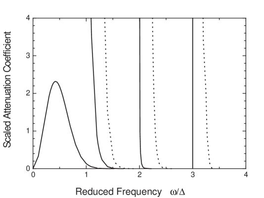
FIG. 2.: Scaled attenuation coefficient $(W^{4}/\delta^{2}aL)|\sigma_{-n,m}|^{2}$ as a function of reduced frequency, $\omega/\Delta$ where $\Delta=\pi c/W$ with $c$ the average velocity of the elastic waves: solid - from mode $m=0$ to mode $-n$, $n=0..3$ and dashed - mode $m$ to mode $-m$, $m=1..3$. A value of the roughness correlation length $a=0.75W$ was used.

At low enough temperatures only the lowest mode with $k_{0}=\omega/c$ contributes to the thermal conductance, and only the backscattering of this mode given by Eq. (31) reduces the conductance below the universal value. This reduction is plotted as a function of the temperature scaled by $\hbar c/k_{B}a$ in Fig. 3. The temperature of maximum reduction depends on the roughness correlation length $a$, whereas both the roughness amplitude and correlation length change the magnitude of the reduction. For small roughness, we can expand the exponential term in Eq. (30) and at low temperatures only small $\omega$ contributes to the integral so that the Gaussian factor may be replaced by unity, ${\exp[}-a^{2}\omega^{2}/c^{2}]\simeq 1$. This leads to

$$\frac{K}{T}\simeq\frac{\pi^{2}k_{B}^{2}}{3h}\left[1-\frac{8\pi^{9/2}}{5}\frac{\delta^{2}aL}{W^{4}}\left(\frac{k_{B}T}{\hbar\Delta}\right)^{2}\right],$$ (32)

where $\Delta=\pi c/W$ is the spacing between the mode cutoff frequencies. Thus at low temperatures, the conductance divided by temperature should show a quadratic temperature decrease with an amplitude depending on the combination of roughness parameters $\delta^{2}a/W^{3}$.

IV Comparison with experiment

To compare with the experiments of Schwab et al.[4] we use the following geometry and material parameters. We take a wave guide structure of rectangular cross section with width $W=160$ nm and length $L=1$ $\mu$m. In the experimental geometry the width varied along the length to provide smooth junctions with the reservoirs. This was done to eliminate scattering off abrupt changes in the geometry. We use the width at the narrowest point as our estimate. For the length we use the length of the central portion over which the width is fairly constant. Since the length only occurs in the combination $\delta^{2}L$, changing the value of $L$ used will only change the estimated value of $\delta$. We use a wave propagation speed $c=8250$ m/s which is the average of the velocity of longitudinal and transverse elastic waves in silicon nitride.

The roughness parameters are not known a priori. As a first attempt we might try to estimate the combination $\delta^{2}aL/W^{4}$ from the quadratic decrease in the thermal conductance at low temperatures, Eq. (32). This would give the value $a\delta^{2}L/W^{4}\sim 0.05$. However, from Fig. 3 we see that the quadratic low-temperature fit is only good up to about a quarter of the temperature of the maximum backscattering of the first mode. If we estimate this temperature from the minimum in the measured conductance, we find that the data does not extend to low enough temperatures to provide a reliable fit, and so this value can only be used as an order of magnitude. In fact our “best fit” (see below) over temperatures up to $1$ K corresponds to a value $a\delta^{2}L/W^{4}$ about a factor of $4$ larger

It is interesting to use this value of the roughness parameters to estimate the strength of the scattering of the higher modes. For example, for the first mode, with cutoff frequency $\Delta$, and at a wave vector $\pi/W$ corresponding to a frequency $\sqrt{2}\Delta$ we find for the backscattering into the same mode

$$\gamma_{1}(k_{1}=\pi/W)L\sim 16\exp\left(-\pi^{2}a^{2}/W^{2}\right).$$ (33)

The scattering increases for smaller wave vectors, diverging at onset as shown in Fig. 2. Remember that the transmission amplitude is $e^{-\gamma_{1}L}$. This means that the scattering of the higher modes is strong over the $1\mu$ length, unless sufficiently reduced by the exponential factor arising from the reduced roughness at short length scales. To fit the higher temperature data using Eq. (30) we will find that we need a value of $a$ comparable to $W$. Although this strongly reduces the value of $\gamma_{1}(k_{1}=\pi/W)$, there remain frequency ranges where the scattering of this mode and other modes is strong. An interesting consequence is that a significant fraction of the thermally excited phonons at temperatures of order $1$ K are predicted to be localized in the experiments of Schwab et al., with a localization length less than the length of the bridge. Unfortunately, in this regime the estimate of the contribution to the conductance from these modes predicted by our lowest order scattering calculation, will not be accurate.

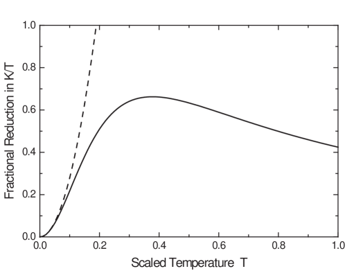
FIG. 3.: Reduction in the thermal conductance divided by temperature due to back scattering of the lowest mode, expressed as the ratio to the universal conductance divided by temperature and then scaled by $aW^{2}/\delta^{2}L$, as a function of temperature scaled by $\hbar c/k_{B}a$.

From Fig. 3 we can suggest two mechanisms that might account for the observed minimum in the dependence of $K/T$ on temperature. The first mechanism ascribes the minimum in $K/T$ to the behavior of the first mode alone, as plotted in Fig. 3. The upturn in $K/T$ arises from the reduced scattering of the lowest mode as the wave vectors of the important modes increase with temperature. The second mechanism supposes that the scattering of the lowest mode is responsible for the decreasing $K/T$ at low temperatures, but that the subsequent increase is from the thermal excitation of the higher modes. For our “best fit” values of $a,\delta$ (see below) the results are summarized in Fig. 4. The picture is quite complicated, with both the reduced scattering of the lowest mode and the thermal excitation of the higher modes contributing to the rise in $K/T$ with increasing temperature. Furthermore, due to the strong scattering of the higher modes near their cutoff frequencies, these modes become important in the transport at a higher temperature than would be estimated simply from their cutoff frequencies. The higher modes excited near their threshold frequencies are localized and do not contribute significantly to the transport.

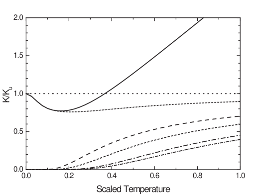
FIG. 4.: Contributions to the thermal conductance $K$ divided by the universal value $K_{u}$ from the first few modes for the ideal no scattering case, and for the rough case with scattering as a function of the scaled temperature $k_{B}T/\hbar\Delta$: solid line - total thermal conductance for the rough surface case; dotted line and short-dotted line - conductance of mode 0 (ideal and rough); dashed line and short-dashed line - conductance of mode 1 (ideal and rough); dash-dotted line and short-dash-dotted line - conductance of mode 2 (ideal and rough). Values of the roughness parameters were $a/W=0.75$ and $\delta/W=0.22$.

In Fig. 5 the thermal conductance calculated using Eq. (30) is plotted together with the ideal (no-scattering) conductance and the measurements of Schwab et al. The conductance is scaled such that the universal conductance appears as unity. The roughness parameters $a/W=0.75$ and $\delta/W=0.22$ (so that $a\delta^{2}L/W^{4}=0.23$) were used, and yield a reasonable fit to the data. Our $2D$ model shows the same trend as the experimental data: a decrease in the thermal conductance below the universal value at low temperatures where only the lowest modes are excited, then a gradually increasing conductance as other modes are excited and the scattering of the lowest mode is reduced. Comparison to the ideal (non-scattering) curve shows that the scattering is important over the whole temperature range examined $(T<1$ K$)$. These values of $\delta=35$ nm and $a=120$ nm appear reasonable when one considers the physical process of constructing the mesoscopic bridge structure. For example, a typical chemical etch of silicon nitride can easily produce a few tens of nm in roughness amplitude. Electron micrographs of the actual structure used in the experiment[7] show roughness on scales comparable to the ones we estimate.

There are small but systematic differences at very low temperatures, where the conductance is dominated by the lowest modes, and the theory should be most accurate. The discrepancy suggests that we are overestimating the scattering at long wavelengths. A roughness spectrum $\tilde{g}(k)\sim k^{2}e^{-a^{2}k^{2}/4}$ with a reduced amplitude at small wave numbers gives a better fit to the data. Such a form might be physically reasonable, since we might expect the roughness to be largest at a scale of order the minimum dimension of the structure, and reduced at larger scales than this. However, since the scalar model does not account for the mode structure of the elastic beam accurately, it is probably unwise to use the discrepancies in Fig. 5 to make any firm deductions. Such conclusions must await a more accurate treatment of the modes within elasticity theory.

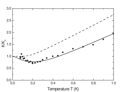
FIG. 5.: Thermal conductance relative to the universal value $K_{u}$ as a function of temperature for the ideal case (dotted line), the rough surface case (solid line), and the data of Schwab et al. (circles). The roughness parameters used were $a/W=0.75$, $\delta/W=0.22$.

V Conclusion

We have investigated the cause of the thermal conductance decrease below the universal value at low temperatures by employing a Green function approach to calculate the reduced transmission of the elastic waves due to surface roughness, and then using Landauer’s formula for the thermal conductance.

At low temperatures, the conductance divided by the temperature is dominated by the lowest mode. The scattering of this mode reduces the conductance below the universal value with a quadratic dependence on temperature for low temperatures with an amplitude proportional to the combination of roughness parameters $a\delta^{2}$. As the temperature increases, higher modes begin to play a role and the scattering of the lowest modes is reduced, so that the conductance increases. We find that the effect of scattering is always significant, reducing the conductance below the ideal ballistic value over the whole temperature range we investigate $T<1$ K. Considering the simplicity of our model our results agree well with the experiment of Schwab et al. In future work we will present results for a full elastic theory treatment of the thin bridge.

- [1] D.E. Angelescu M.C, Cross, and M.L. Roukes Superlattice and Microstructure, 23, 673 (1998).
- [2] L.C. Rego and G. Kirczenow, Phys. Rev. Lett. 81, 232 (1998).
- [3] M.P. Blencowe, Phys. Rev. B 59, 4992 (1999).
- [4] K. Schwab, E. A. Henriksen, J. M. Worlock, M. L. Roukes, Nature 404, 974 (2000).
- [5] A. Kambili, G. Fagas, V. I. Fal’ko, and C. J. Lambert, Phys. Rev. B. 60, 15593 (1999).
- [6] S.V. Biryukov, Yu.B. Gulyaev, V.V. Krylov, V.P. Plessky, Surface Acoustic Waves in Inhomogeneous Media, Springer-Verlag, Berlin (1995).
- [7] K. Schwab, Private communication