Tunneling conductance of SIN junctions with different gap symmetries
and non-magnetic impurities
by direct solution of real-axis Eliashberg equations

Abstract

We theoretically investigate the effect of various symmetries of the superconducting order parameter $\Delta(\omega)$ on the normalized tunneling conductance of SIN junctions by directly solving the real-axis Eliashberg equations (EEs) for a half-filled infinite band, with the simplifying assumption $\mu^{\ast}$ = 0. We analyze six different symmetries of the order parameter: $s$, $d$, $s+{\rm i}d$, $s+d$, extended $s$ and anisotropic $s$, by assuming that the spectral function $\alpha^{2}F(\Omega)$ contains an isotropic part $\alpha^{2}F(\Omega)_{{\rm is}}$ and an anisotropic one, $\alpha^{2}F(\Omega)_{{\rm an}}$, such that $\alpha^{2}F(\Omega)_{{\rm an}}$=$g\cdot\alpha^{2}F(\Omega)_{{\rm is}}$, where $g$ is a constant.

We compare the resulting conductance curves at $T=2$ K to those obtained by analytical continuation of the imaginary-axis solution of the EEs, and we show that the agreement is not equally good for all symmetries. Then, we discuss the effect of non-magnetic impurities on the theoretical tunneling conductance curves at $T=4$ K for all the symmetries considered.

Finally, as an example, we apply our calculations to the case of optimally-doped high-$T_{\mathrm{c}}$ superconductors. Surprisingly, although the possibility of explaining the very complex phenomenology of HTSC is probably beyond the limits of the Eliashberg theory, the comparison of the theoretical curves calculated at $T$=4 K with the experimental ones obtained in various optimally-doped copper-oxides gives fairly good results.

I Introduction

The semi-phenomenological Migdal-Eliashberg theory Eliashberg has been successfully used in the past to describe many properties of low-$T_{\rm c}$ superconductors. For example, it has provided a quite precise explanation of the tunneling experimental data obtained on almost all the conventional superconductors. In most of these cases, theoretical predictions in good agreement with the experimental results have been obtained by solving the Eliashberg equations (EEs) for an $s$-wave order parameter. However, other symmetries of the order parameter may exist. It is therefore interesting to study how, in the framework of this theory, the gap symmetry influences the theoretical conductance curves.

In this paper, we will calculate the theoretical normalized conductance curves of SIN junctions for various gap symmetries ($s$, $d$, $s+{\rm i}d$, $s+d$, anisotropic $s$ and extended $s$) VanHarlingen by directly solving the real-axis Eliashberg equations (EEs) in the half-filling case.

Incidentally, this procedure is much more complicated than the usual one, which consists in solving the EEs in the imaginary-axis formulation and then continuing the solution to the real axis. Nevertheless, it is much more general and can be used at every temperature, whilst the second approach is meaningful only at very low temperatures (in principle, $T\rightarrow 0$). Moreover, we will show that, at a finite but still very low temperature ($T$ = 2 K) the imaginary-axis procedure gives results whose agreement with those directly obtained from the real-axis EEs is not equally good for all symmetries.

We will also present the theoretical conductance curves obtained at various temperatures, and with increasing values of the coupling constant. It will be shown that large values of the isotropic coupling constant produce some characteristic and well-recognizable features of the normalized conductance curves, which are actually observed experimentally.

Moreover, we will investigate the effect of different amounts of non-magnetic impurities, in both the unitary and non-unitary limits, on the tunneling normalized conductance curves, and discuss the results for all the symmetries of the order parameter.

Finally, we will try a comparison of the theoretical tunneling curves with experimental data appeared in literature and concerning some high-$T_{\rm c}$ compounds.

II Eliashberg equations for different pair symmetries

In this section we calculate the theoretical normalized conductance for a tunnel junction within the framework of Migdal-Eliashberg theory. To do so, we solve the generalized real-axis EEs Eliashberg ; Carbotte ; AllenMitr for the renormalization function $Z(\omega,{\bf k})$ and the order parameter $\Delta(\omega,{\bf k})$. As well known, in the real-axis formalism the EEs take the form of a set of coupled integral equations, whose kernels contain the retarded electron-boson interaction $\alpha^{2}F(\Omega,{\bf k},{\bf k}^{\prime})$, the Coulomb pseudopotential $\mu^{\ast}\left({\bf k},{\bf k}^{\prime}\right)$, and the energy of the carriers $\varepsilon_{{\bf k}}$, measured with respect to the bare band chemical potential Rieck ; Strinati ; JiangCarb . In the following, we will use a single-band approximation, and we will restrict our discussion to the 2-dimensional case, thus referring, for example, to the $ab$ planes of layered superconductors and neglecting the band dispersion and the gap in the $c$ direction. For simplicity, we will assume that the Fermi surface is a circle in the $ab$ plane Rieck and that the wavevectors ${\bf k}$ and ${\bf k}^{\prime}$ are completely determined by the respective azimuthal angles $\phi$ and $\phi^{\prime}$, since their length is, as usual, taken equal to k_F.

To allow for different symmetries of the pair state, we expand the superconducting spectral function $\alpha^{2}F(\Omega,\phi,\phi^{\prime})$ and the Coulomb pseudopotential $\mu^{\ast}(\phi,\phi^{\prime})$ in terms of basis functions $\psi_{{\rm is}}$ and $\psi_{{\rm an}}$, where the subscripts mean isotropic and anisotropic, respectively. At the lowest order we suppose $\alpha^{2}F(\Omega,\phi,\phi^{\prime})$ and $\mu^{\ast}(\phi,\phi^{\prime})$ to contain separated isotropic and anisotropic contributions, as in the following expressions:

$$\alpha^{2}F(\Omega,\phi,\phi^{\prime})=\alpha^{2}F(\Omega)_{{\rm is}}\psi_{{\rm is}}\left(\phi\right)\psi_{{\rm is}}\left(\phi^{\prime}\right)+\alpha^{2}F(\Omega)_{{\rm an}}\psi_{{\rm an}}\left(\phi\right)\psi_{{\rm an}}\left(\phi^{\prime}\right)$$ (1)

$$\mu^{\ast}(\phi,\phi^{\prime})=\mu_{{\rm is}}^{\ast}\psi_{{\rm is}}\left(\phi\right)\psi_{{\rm is}}\left(\phi^{\prime}\right)+\mu_{{\rm an}}^{\ast}\psi_{{\rm an}}\left(\phi\right)\psi_{{\rm an}}\left(\phi^{\prime}\right).$$ (2)

The basis function $\psi_{{\rm is}}\left(\phi\right)$ and $\psi_{{\rm an}}\left(\phi\right)$ are chosen as follows:

$$\psi_{{\rm is}}\left(\phi\right) = 1$$

$$\psi_{{\rm an}}\left(\phi\right) = \left\{\begin{array}[]{l}\sqrt{2}\cos\left(2\phi\right)\\ 8\sqrt{2/35}\cos^{4}\left(2\phi\right)\\ 2\sqrt{2/3}\cos^{2}\left(2\phi\right)\end{array}\right.\hskip 28.45274pt\begin{array}[]{l}(d-wave)\\ (anisotropic~{}\emph{s})\\ (extended~{}\emph{s})\end{array}$$ (9)

We search for solutions of the EEs having the form:

$$\Delta(\omega,\phi) = \Delta_{{\rm is}}(\omega)\pm\Delta_{{\rm an}}(\omega)\psi_{{\rm an}}\left(\phi\right)$$ (10)

$$Z(\omega,\phi) = Z_{{\rm is}}(\omega)\pm Z_{{\rm an}}(\omega)\psi_{{\rm an}}\left(\phi\right).$$

We assume as an “ansatz” that the negative sign in the above expressions is used only for the extended s-wave symmetry, while in all other cases the positive sign is chosen. In doing so one recovers in the BCS limit the form of $\Delta$ given in Ref.VanHarlingen . Notice that the choice of the sign in the expression for $Z(\omega,\phi)$ has no effect. In fact, using eqs.(10) makes the Eliashberg equations for $\Delta(\omega,\phi)$ and $Z(\omega,\phi)$ split into four equations for $\Delta_{{\rm is}}(\omega)$, $Z_{{\rm is}}(\omega)$, $\Delta_{{\rm an}}(\omega)$ and $Z_{{\rm an}}(\omega)$. The equation for $Z_{{\rm an}}(\omega)$ is a homogeneous integral equation whose only solution in the weak-coupling regime is $Z_{{\rm an}}(\omega)\equiv 0$. Even though in the strong-coupling limit a non-zero solution could exist above a certain coupling strength threshold, we do not consider here this rather exotic case and then we assume that the stable solution corresponds to $Z_{{\rm an}}(\omega)\equiv 0$ for all couplings Musaelian ; JohnRenato . Consequently, we will not write the equation for $Z_{{\rm an}}(\omega)$.

In writing the remaining equations for $\Delta_{{\rm is}}(\omega)$, $Z_{{\rm is}}(\omega)$, $\Delta_{{\rm an}}(\omega)$, we insert an additional term which takes into account the presence of non-magnetic impurities JiangCarbDynes . Actually, in the following numerical solutions we will consider this term only where explicitly specified, and we will disregard it otherwise. The EEs are then written in the form:

$$\Delta_{{\rm is}}(\omega)Z_{{\rm is}}(\omega) = \frac{1}{2\pi}\int_{0}^{2\pi}{\rm d}\phi\int_{0}^{+\infty}\mathrm{Re}\left[P_{{\rm is}}(\omega^{\prime},\phi)\right]\left[K_{{\rm is+}}(\omega,\omega^{\prime},\phi)-\mu_{{\rm is}}^{\ast}\theta\left(\omega_{c}-\omega^{\prime}\right)\right]{\rm d}\omega^{\prime}$$ (11)

$$+{\rm i}\pi\Gamma\frac{\overline{P}_{{\rm is}}(\omega)}{C^{2}+\overline{P}_{{\rm an}}^{2}(\omega)+\overline{P}_{{\rm is}}^{2}(\omega)+\overline{N}_{{\rm is}}^{2}(\omega)}$$

$$\Delta_{{\rm an}}(\omega)Z_{{\rm is}}(\omega) = \frac{1}{2\pi}\int_{0}^{2\pi}{\rm d}\phi\int_{0}^{+\infty}\mathrm{Re}\left[P_{{\rm an}}(\omega^{\prime},\phi)\right]\left[K_{{\rm an+}}(\omega,\omega^{\prime},\phi)-\mu_{{\rm an}}^{\ast}\theta\left(\omega_{c}-\omega^{\prime}\right)\psi_{{\rm an}}\left(\phi\right)\right]{\rm d}\omega^{\prime}$$ (12)

$$+{\rm i}\pi\Gamma\frac{\overline{P}_{{\rm an}}(\omega)}{C^{2}+\overline{P}_{{\rm an}}^{2}(\omega)+\overline{P}_{{\rm is}}^{2}(\omega)+\overline{N}_{{\rm is}}^{2}(\omega)}$$

$$\left[1-Z_{{\rm is}}(\omega)\right]\omega = \frac{1}{2\pi}\int_{0}^{2\pi}{\rm d}\phi\int_{0}^{+\infty}\mathrm{Re}\left[N_{{\rm is}}(\omega^{\prime},\phi)\right]K_{{\rm is-}}(\omega,\omega^{\prime},\phi){\rm d}\omega^{\prime}$$

$$-{\rm i}\pi\Gamma\frac{\overline{N}_{{\rm is}}(\omega)}{C^{2}+\overline{P}_{{\rm an}}^{2}(\omega)+\overline{P}_{{\rm is}}^{2}(\omega)+\overline{N}_{{\rm is}}^{2}(\omega)}.$$

where $\omega_{{\rm c}}$, which appears in eqs.(11, 12), is a cutoff energy, and the functions $P_{\rm is}(\omega,\phi)$, $P_{\rm an}(\omega,\phi)$ and $N_{\rm is}(\omega,\phi)$ are defined as follows:

$$P_{{\rm is}}(\omega,\phi)=\frac{\Delta_{{\rm is}}(\omega)}{\sqrt{\omega^{2}-\left[\Delta_{{\rm is}}(\omega)+\Delta_{{\rm an}}(\omega)\psi_{{\rm an}}\left(\phi\right)\right]^{2}}}$$ (14)

$$P_{{\rm an}}(\omega,\phi)=\frac{\Delta_{{\rm an}}(\omega)\psi_{{\rm an}}\left(\phi\right)}{\sqrt{\omega^{2}-\left[\Delta_{{\rm is}}(\omega)+\Delta_{{\rm an}}(\omega)\psi_{{\rm an}}\left(\phi\right)\right]^{2}}}$$ (15)

$$N_{{\rm is}}(\omega,\phi)=\frac{\omega}{\sqrt{\omega^{2}-\left[\Delta_{{\rm is}}(\omega)+\Delta_{{\rm an}}(\omega)\psi_{{\rm an}}\left(\phi\right)\right]^{2}}}$$ (16)

while

$$\overline{P}_{\rm is,an}(\omega)=\frac{1}{2\pi}\int_{0}^{2\pi}P_{\rm is,an}(\omega,\phi)\>{\rm d}\phi$$ (17)

and

$$\overline{N}_{\rm is}(\omega)=\frac{1}{2\pi}\int_{0}^{2\pi}N_{\rm is}(\omega,\phi)\>{\rm d}\phi.$$ (18)

The functions $K_{{\rm is,an\pm}}(\omega,\omega^{\prime},\phi)$ in the integral over $\omega^{\prime}$ are given by

$$K_{{\rm is,an\pm}}(\omega,\omega^{\prime},\phi) = \int_{0}^{+\infty}{\rm d}\Omega\>\alpha^{2}F(\Omega)_{{\rm is,an}}\>\psi_{{\rm is,an}}\left(\phi\right)\cdot$$

$$\left[\frac{f\left(-\omega^{\prime}\right)+n\left(\Omega\right)}{\Omega+\omega^{\prime}+\omega+{\rm i}\delta}\pm\frac{f\left(-\omega^{\prime}\right)+n\left(\Omega\right)}{\Omega+\omega^{\prime}-\omega-{\rm i}\delta}\mp\frac{f\left(\omega^{\prime}\right)+n\left(\Omega\right)}{\Omega-\omega^{\prime}+\omega+{\rm i}\delta}\mp\frac{f\left(\omega^{\prime}\right)+n\left(\Omega\right)}{\Omega-\omega^{\prime}-\omega-{\rm i}\delta}\right]$$

where $f\left(\omega\right)$ and $n\left(\Omega\right)$ are the Fermi and Bose distributions, respectively.

As anticipated above, the last term on the right-hand side of equations (11-II) allows for the contribution of scattering from impurities. It contains the parameters $\Gamma$ and $C$ which are defined through the relations $\Gamma=n_{{\rm I}}/N(0)\pi^{2}$ and $C$=$\cot(\delta_{0})$, where $n_{{\rm I}}$ is the impurity concentration, $N(0)$ is the value of the normal DOS at the Fermi energy and $\delta_{0}$ is the scattering phase shift JiangCarbDynes .

Notice that, in the case we want to obtain a $s+{\rm i}d$ solution, we simply need to replace the denominator of $P_{{\rm an}}(\omega,\phi)$, $P_{{\rm is}}(\omega,\phi)$ and $N_{\rm is}(\omega,\phi)$ with $\sqrt{\omega^{2}-\left[\Delta_{{\rm s}}^{2}(\omega)+\Delta_{{\rm d}}^{2}(\omega)\psi^{2}_{{\rm d}}\left(\phi\right)\right]}$, where the generic subscripts ‘is’ and ‘an’ have been replaced by ‘s’ and ‘d’, respectively.

To simplify the problem of numerically solving these equations, we put $\alpha^{2}F(\Omega)_{{\rm an}}=g\cdot\alpha^{2}F(\Omega)_{{\rm is}}$ where $g$ is a constant JohnRenato ; Dolgov . As a consequence, the electron-boson coupling constants for the isotropic-wave channel and the anisotropic-wave one, which are given by $\lambda_{{\rm is}}$=$2\int_{0}^{+\infty}{\rm d}\Omega\>\alpha^{2}F(\Omega)_{{\rm is}}/\Omega$ and $\lambda_{{\rm an}}$=$\left(1/\pi\right)\int_{0}^{2\pi}{\rm d}\phi\>\psi_{{\rm an}}^{2}\left(\phi\right)\int_{0}^{+\infty}{\rm d}\Omega\>\alpha^{2}F(\Omega)_{{\rm an}}/\Omega$ respectively, result to be proportional: $\lambda_{{\rm an}}=g\cdot\lambda_{{\rm is}}$.

The real-axis generalized Eliashberg equations (11-II) are numerically solved by using an iterative procedure, which stops when the real and imaginary values of the functions $\Delta_{{\rm is}}(\omega),$ $\Delta_{{\rm an}}(\omega)$ and $Z_{{\rm is}}(\omega)$ at a new iteration differ less than $1\cdot 10^{-3}$ with respect to the previous ones. This usually happens after a number of iterations between 10 and 15.

By starting from the real-axis solutions $\Delta_{{\rm is}}(\omega)$ and $\Delta_{{\rm an}}(\omega)$, we then calculate the normalized conductance $G_{\rm n}(V)$ of a tunnel junction, which is given by the convolution of the quasiparticle density of states $N(\omega)=\mathrm{Re}\left[\mathrm{sgn}(\omega)\overline{N}_{\rm is}(\omega)\right]$ with the Fermi distribution function:

$$\vspace{-2mm}G_{\rm n}(V)=\frac{1}{e}\int_{-\infty}^{+\infty}{\rm d}\omega\>N(\omega+eV)\cdot\left[f(\omega)-f(\omega+eV)\right].\vspace{1mm}$$ (20)

Of course, this is the simplest possible choice. We are aware that, when anisotropic superconductors are involved, the normalized conductance should have a much more complex form to take into account its dependence on the junction’s geometry and on some other factors such as, for example, the direction of the incident current and the angle $\alpha$ between the normal to the interface and the crystallographic $a$ axis Tanaka . Here we restrict ourselves to the simplest case of plane interface and normal current and we also put $\alpha=0$.

The main features of the resulting $G_{\rm n}(V)$ curves will be discussed in the following sections.

As already pointed out in the introduction, the direct numerical solution of the real-axis EEs described so far is a quite complicated and time-consuming procedure. However, as well known, the EEs admit an imaginary-axis formulation, in which integrals are replaced by summations over the integer index of the so-called Matsubara frequencies $\omega_{{\rm n}}$. The numerical solution of the EEs in this formalism is therefore a much simpler task, which gives the real discrete functions $\Delta\left({\rm i}\omega_{{\rm n}}\right)$ and $Z({\rm i}\omega_{{\rm n}})$, that can be analytically continued to the real axis by means of Padé approximants VidbergSerene . In principle, this analytical continuation is meaningful only at very low temperatures. Therefore, one could wonder if, and in what temperature range, this method is able to give results in accordance with those obtained by starting from the real-axis EEs. A comparison between the density of states (DOS) obtained by the two techniques was made for the $s$-wave symmetry and for small values of the coupling constant ($\lambda<2$) VidbergSerene , and a substantial agreement was found. Here we compare the normalized tunneling conductance curves calculated at $T=2$ K not only in the $s$-wave symmetry for greater values of $\lambda$, but also in the other symmetries analyzed here. The results will be discussed in the next section.

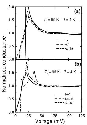
Figure 1: Theoretical normalized conductance curves for $\mu^{*}\>$= 0 at $T\>$= 4 K in various symmetries of the order parameter: s, d, s+id (a) and s+d,  extended s, anisotropic s (b).

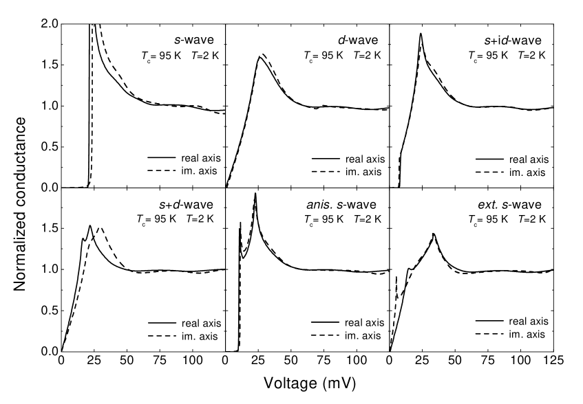
Figure 2: Comparison of the normalized tunneling conductance curves obtained from the real-axis solution of the Eliashberg equations, with those obtained by the analytical continuation of the imaginary-axis solutions, at $T$=2 K, in all the symmetries considered.

III Theoretical Results

The numerical solution of the EEs (11)-(II) requires the knowledge of the function $\alpha^{2}F(\Omega)_{\rm is}$ which appears in the expressions of $K_{\rm is,an\pm}$ and $\lambda_{\rm is,an}$. Even though we are not referring to a particular material, we can make a choice for $\alpha^{2}F(\Omega)_{\rm is}$ by taking advantage of the fact that its detailed shape has little influence on the final solution, which instead depends, as observed elsewhere Varelogiannis2 , on the quantity $\omega_{\log}=$ $\exp\left(\frac{2}{\lambda}\int_{0}^{+\infty}d\Omega\frac{\alpha^{2}F\left(\Omega\right)}{\Omega}\ln\Omega\right)$. Since in this section we are only interested in calculating theoretical curves, we can take:

$$\alpha^{2}F(\Omega)_{{\rm is}}=\frac{\lambda_{{\rm is}}}{\lambda}\alpha^{2}F(\Omega)_{{\rm Bi2212}}.$$ (21)

Here $\alpha^{2}F(\Omega)_{{\rm Bi2212}}$ is the electron-boson spectral function determined in a previous paper by inversion of the $s$-wave EEs starting from tunneling data obtained on Bi₂Sr₂CaCu₂O_8+δ (Bi-2212) break junctions PhysC97 , and $\lambda$ is the corresponding coupling constant. The values of $\lambda_{\rm is}$ and that of $\lambda_{\rm an}$ are chosen to have $T_{\rm c}\equiv\max(T_{\rm c}^{\mathrm{is}},T_{\rm c}^{\mathrm{an}})$ = 95 K (which, in most of our calculations, is chosen as a representative value for high-$T_{\rm c}$ superconductors).

From now on, we will put the Coulomb pseudopotential $\mu^{\ast}$ to zero in all the equations of the previous section. It will be shown in the next section that this does not limit the generality of the results.

As already pointed out, we search for a solution of the real-axis Eliashberg equations which contains an isotropic and an anisotropic part, as shown in equation (10). Actually, the choice of the coupling constants $\lambda_{{\rm is}}$ and $\lambda_{{\rm an}}$ to be used for the numerical solution can affect the symmetry of the order parameter $\Delta(\omega,\phi)$, which can show either pure isotropic-wave or anisotropic-wave symmetry, or a mixed symmetry. Moreover, for some particular values of the coupling constants, the final symmetry of the order parameter depends on the starting values of $\Delta_{{\rm is}}(\omega)$ and $\Delta_{{\rm an}}(\omega)$.

Results with the expected symmetry, and compatible with the value of the critical temperature we have chosen above ($T_{{\rm c}}$= 95 K) are obtained with the values of the coupling constants reported in Table I, where also the corresponding isotropic and anisotropic critical temperatures are shown.

symmetry	$\lambda_{\rm is}$	$\lambda_{\rm an}$	$T_{\rm c}^{\mathrm{is}}$ (K)	$T_{\rm c}^{\mathrm{an}}$ (K)
s	3.15	-	95	-
d	2	2.3	-	95
s+id	2	2.3	66	95
s+d	1.25	1.74	40	95
anis. s	2	2.29	63	95
ext. s	1	1.54	32	95

Table 1: Values of the coupling constants used in the calculations of Section III and corresponding critical temperatures for all the gap symmetries considered.

It is worthwhile to remark that, in all cases apart from the $s$-wave one, different couples of $\lambda_{{\rm is}}$ and $\lambda_{{\rm an}}$ values can give rise to the same critical temperature and the same symmetry and, therefore, Table I only presents one of the possible choices. These coupling constants will be used in all the calculations presented in this section.

Figure 1 reports the theoretical normalized tunneling conductance curves $G_{\rm n}(V)$ at $T=4$ K in the six different symmetries analyzed (the corresponding values of the coupling constants are those reported above). In all the symmetries apart from the $s$-wave one, a conductance excess below the gap is obtained. However, in all cases the normalized conductance is zero at zero voltage. As we will discuss later, the zero-bias anomaly which is often experimentally observed could in fact be reproduced, in the framework of the Eliashberg theory, by taking into account the scattering from impurities, which has been disregarded here.

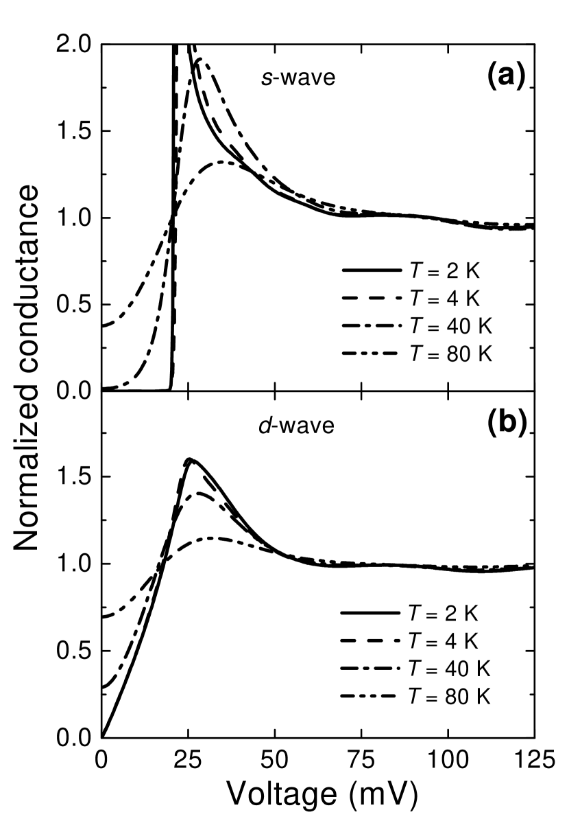
Figure 3: Theoretical normalized conductance curves for $\mu^{\ast}\>$= 0 at $T$=2, 4, 40 and 80 K in the $s$-wave symmetry (a) and in the $d$-wave symmetry (b).

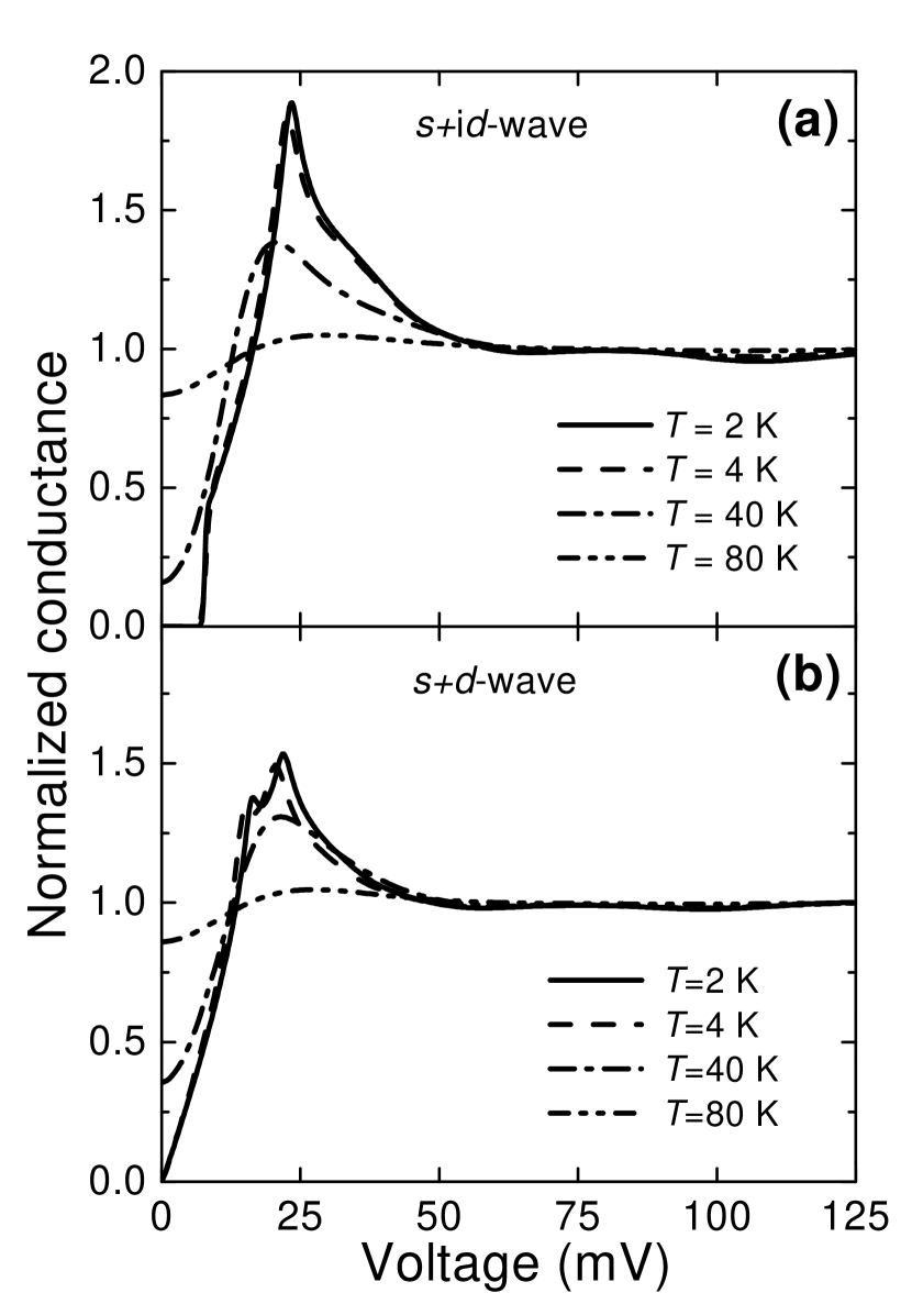
Figure 4: Theoretical normalized conductance curves for $\mu^{\ast}\>$= 0 at $T$=2, 4, 40 and 80 K in the $s$+i$d$-wave symmetry (a) and in the $s$+$d$-wave symmetry (b).

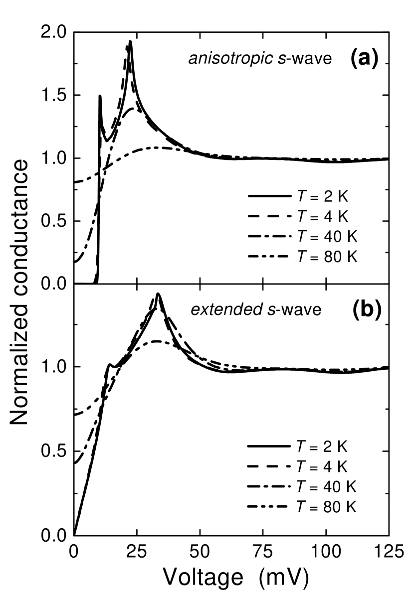
Figure 5: Theoretical normalized conductance curves for $\mu^{\ast}\>$= 0 at $T$=2, 4, 40 and 80 K in the anisotropic $s$-wave symmetry (a) and in the extended $s$-wave symmetry (b).

As anticipated in the previous section, our choice of directly solving the real-axis EEs can be motivated by the fact that the analytical continuation of the solutions $\Delta({\rm i}\omega_{n})$ and $Z({\rm i}\omega_{\rm n})$ of the EEs in the imaginary-axis formulation is correct only at very low temperature. The meaning of this ‘very low’ can be clarified by comparing the results of the two approaches at various temperatures. The result of such a comparison is that, even at the liquid helium temperature

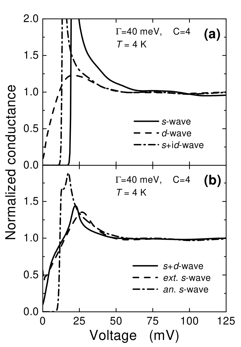
Figure 6: Theoretical normalized conductances curves at $T\>$=4 K in various gap symmetries, for $\mu^{\ast}\>$= 0 and in the presence of scattering from impurities in the non-unitary limit ($\Gamma$ = 40 meV and $C$ = 4).

temperature (at which most of the experimental data are obtained), the analytical continuation gives rise to some sensible deviations from the real-axis solution. As shown in Fig. 2, at a lower temperature ($T=2$ K), the agreement between the theoretical $G_{\rm n}(V)$ curves obtained by the two procedures is good for the $d$-wave, $s+\mathrm{i}d$-wave and anisotropic s-wave symmetries. In the extended $s$ case, the ‘imaginary-axis’ curve agrees very well with the ‘real-axis’ one, except that in the low-voltage regime. In the ($s+d$)-wave symmetry, the peak of the imaginary-axis solution is broader than that of the real-axis one, and displaced of about +8 mV. Finally, in the $s$-wave case, the analytical continuation does not work well, since a shift of +3 mV of the conductance curve is produced. Further checks demonstrate that the agreement gets worse at the increase of $\lambda$, while for sufficiently small values of the coupling constant ($\lambda<2$) the two curves coincide, as found in Ref. VidbergSerene .

Let us now discuss what happens to the conductance curves when the temperature is increased. Figures 3, 4 and 5 show the normalized tunneling conductance curves calculated for all the symmetries at $T$ = 2, 4, 40, 80 K. In general, as expected, increasing the temperature results in a smoothing and broadening of the peaks. The smoothing is particularly evident in the case of the anisotropic $s$ symmetry, in which the low-voltage peak, which is well defined at $T$ = 2 K, is much less evident at 4 K (its height is reduced from 1.5 to 1.25). At the increase of the temperature the curves corresponding to mixed symmetries become more and more similar to one another and to the $d$-wave curve. This is due both to the thermal broadening and to the fact that, with our choices of $\lambda_{\rm is}$ and $\lambda_{\rm an}$, $T_{\rm c}^{\mathrm{is}}$ is always less than $T_{\rm c}^{\mathrm{an}}$ and therefore the isotropic gap component disappears before the anisotropic one. The $s$-wave curve remains instead clearly distinct.

The theoretical curves presented and discussed so far were obtained without inserting in the EEs the additional term taking into account the scattering from non-magnetic impurities. When this effect is allowed for in solving the real-axis EEs, one finds that in the general non-unitary case ($C\neq 0$) it mostly affects the $d$-wave component of the order parameter. By comparing the curves shown in Fig. 6 to those of Fig. 1, we can see that the peak of the $d$-wave tunneling conductance curve is lowered and broadened, while the $s+{\mathrm{i}}d$ curve becomes practically indistinguishable from an $s$-wave one. In the $s+d$ and extended $s$ cases the low-energy peak disappears and a zero-bias is produced, which is greater in the latter case. Finally, in the anisotropic $s$ case the two peaks are closer than in the absence of impurities and the gap is shifted to the left, but the general shape above and below the gap is conserved.

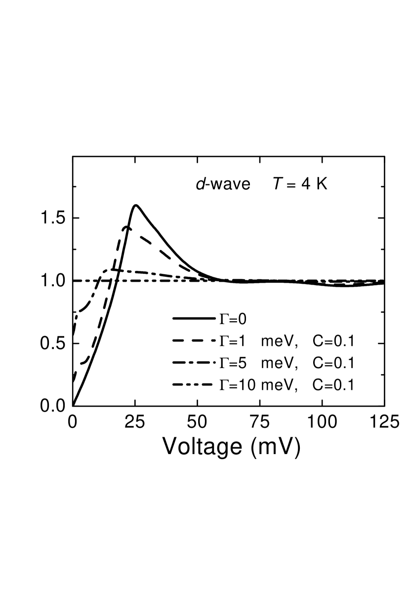
Figure 7: Theoretical normalized conductance curves for $\mu^{*}\>$= 0 in the $d$-wave symmetries at $T$= 4 K with impurities in the unitary limit.

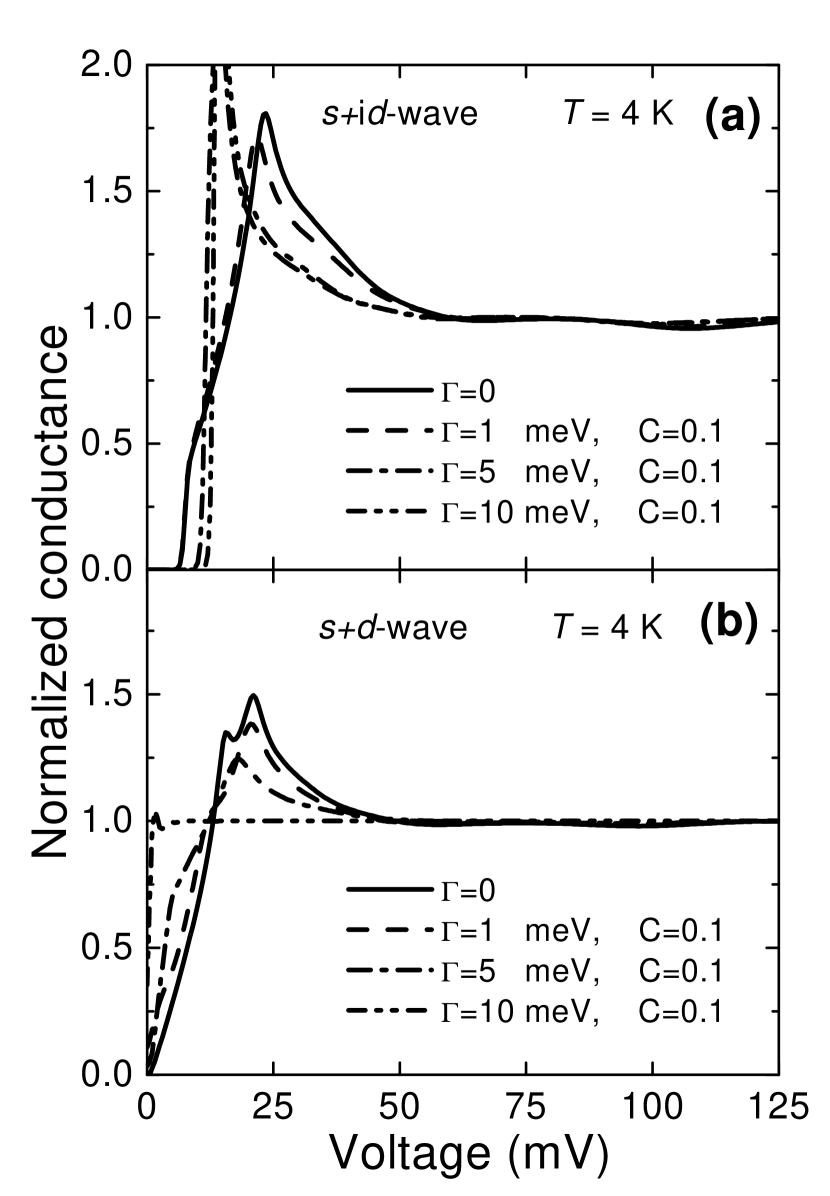
Figure 8: Theoretical normalized conductance curves for $\mu^{*}\>$= 0 in the $s+$i$d$ and $s+d$ symmetries at $T$= 4 K with impurities in the unitary limit.

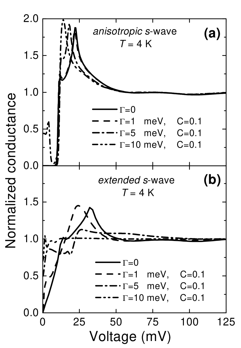
Figure 9: Theoretical normalized conductance curves for $\mu^{*}\>$= 0 in the anisotropic s and extended s symmetries at $T$= 4 K with impurities in the unitary limit.

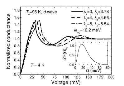
Figure 10: Theoretical $d$-wave conductance curves calculated at $T=4$ K for increasing values of the coupling constants. A suppression of the conductivity at $V\>$=$\>2\Delta_{\rm peak}/e$ (‘dip’) and an enhancement at $V\>$=$\>3\Delta_{\rm peak}/e$ (‘hump’) appear due to the strong electron-boson coupling. The inset shows the isotropic electron-boson spectral function $\alpha^{2}F(\Omega)_{{\rm is}}$ in the $\lambda_{\rm s}=3$ case. In the other cases the curve is simply scaled along the vertical axis. The anisotropic spectral function is $\alpha^{2}F(\Omega)_{{\rm an}}=g\cdot\alpha^{2}F(\Omega)_{{\rm is}}$.

In the unitary limit ($C\ll 1$) the presence of impurities has very different effects in the various symmetries, as shown in Figs. 7, 8 and 9 that report the curves obtained with $C=$ 0.1 and $\Gamma$ = 1, 5, 10 meV. Also in this case the results indicate that, as expected, the main effect of non-magnetic impurities is to suppress the $d$-wave contribution. In the $d$-wave case, a small amount of impurities makes the peaks of the tunneling conductance curves to be lowered, broadened and shifted to the left, and for $\Gamma\geq 10$ meV the superconductivity disappears. In the same limit, the $s+$i$d$ and the anisotropic $s$ curves become very similar to a pure $s$-wave, but the peak is shifted toward lower voltages. Finally, the peak of the extended $s$ and $s$+$d$ curves is lowered and broadened and the superconductivity is easily suppressed.

An interesting feature of the theoretical $G_{\rm n}(V)$ curves that occurs for suitable values of the parameters is a suppression of the tunneling conductance at about twice the gap value (usually referred to as the ‘dip’) and a consequent enhancement of conductance which occurs at about three times the gap value (‘hump’). This feature, which has probably its origin in the non-linear character of the EEs, can be theoretically obtained at least in two ways. In a previous paper bandafinita we showed that in $s$- and $d$-wave symmetries it can result from the finiteness of the energy band. In Ref.Varelogiannis , instead, ‘dip’ and ‘hump’ are obtained in the $s$-wave case by using a very large electron-boson coupling constant. Here we extend this result to the $d$-wave symmetry. Actually, in the $\mu^{\ast}=0$ case large values of the coupling constants would increase the critical temperature well beyond its physical value. To conciliate a very strong coupling with the correct $T_{\mathrm{c}}$, the maximum boson energy must be reduced, that is, the electron-boson spectral function must be confined in the low-energy region and, consequently, $\omega_{\mathrm{log}}$ must be kept sufficiently small. Greater (and more plausible) values of $\omega_{\mathrm{log}}$ can be obtained if one also takes $\mu^{\ast}\neq 0$.

In Fig. 10 we report the theoretical $d$-wave conductance curves obtained with $\mu^{\ast}=0.2$ and $\omega_{\rm c}=500$ meV for increasing values of the isotropic coupling constant: $\lambda_{\rm is}=3,4,5$. The corresponding anisotropic coupling constants ($\lambda_{\rm an}=3.78,4.66,5.54$) have been chosen so as to have $T_{\mathrm{c}}^{\mathrm{calc}}\>$= 95 K. The electron-boson spectral function has the form $\alpha^{2}F(\Omega)_{{\rm is}}=b\Omega^{2}exp(-\Omega/c)$ where $c$ =8 meV and $b$ =0.0234, 0.0313, 0.0391 meV^-2 for $\lambda_{\rm is}=3,4,5$. In all cases $\omega_{\rm log}=12.2$ meV, which is consistent with the energy of the first peak in the phonon spectral function of HTSC. It is clearly seen that the conductance curves reported in the figure show a ‘dip’ and a ‘hump’ at approximately $2\Delta_{\rm peak}/e$ and $3\Delta_{\rm peak}/e$.

Features very similar to those discussed so far have been indeed recently observed in the experimental conductance curves of some HTSC and reported in literature dip . Notice that some possible explanations have already been proposed for these effects Abanov ; Combescot .

IV An illustrative application

Up to now we have dealt only with theoretical predictions, given by the Migdal-Eliashberg theory, concerning the conductance curves corresponding to different gap symmetries. We have discussed the effect of the temperature and of the scattering by impurities.

Now we can give an example of how these calculations can be applied to a real physical problem. Actually, the Eliashberg theory has been successfully used to describe most of the low-$T_{\rm c}$ superconductors by using a simple $s$-wave gap symmetry, thus it is not worthwhile to use these compounds to test our model. Moreover, we have performed our calculations in the 2-dimensional case, and therefore we should refer to layered materials. We can attempt a comparison of our theoretical predictions to tunneling conductance curves of SIN junctions involving high-$T_{\rm c}$ superconductors (HTSC). Of course in applying this theory to HTSC, we must take into account that: i) $\alpha_{\rm an}^{2}F(\Omega)$ doesn’t necessarily have to be multiple of $\alpha_{\rm is}^{2}F(\Omega)$; ii) $\mu^{\ast}$ is probably different from zero; iii) as well known, the Fermi surface (FS) of these materials is not a circle; iv) the bandwidth is finite; v) the conductance of the junctions generally depends on geometrical factors which have been disregarded here. Actually, both $\alpha^{2}F(\Omega,\phi,\phi^{\prime})$ and $\mu^{\ast}$ are unknown, and our assumptions are the simplest possible. The hypothesis that the FS is a circle is as well an oversimplification, but it allows obtaining a more handy model. As far as the bandwidth is concerned, we can presume on the basis of recent results that in optimally-doped HTSC $\varepsilon_{\rm F}\gtrsim 400$ meV and therefore the effects of the finiteness of the bandwidth are not so important bandafinita .

In general, the very complex phenomenology of HTSC yields to the conclusion that many features of these compounds are probably beyond the limits of the Eliashberg theory. Then, we don’t expect this theory to provide an explanation for high-$T_{\rm c}$ superconductivity. We will simply try to use our model to obtain, with suitable choices of the parameters, theoretical curves in agreement with experimental tunneling data in optimally-doped Bi₂Sr₂CaCu₂O_8+δ (BSCCO) PhysC97 , YBa₂Cu₃O_7-δ (YBCO) YBCO , Tl₂Ba₂CuO_6+δ (TBCO) TBCO and HgBa₂CuO_4+δ (HBCO) HBCO single crystals. Of course, the spectral function $\alpha^{2}F(\Omega,\phi,\phi^{\prime})$ is unknown. As already pointed out, in the case of BSCCO we can take, according to eq.(21):

$$\alpha^{2}F(\Omega)_{{\rm is}}=\frac{\lambda_{{\rm is}}}{\lambda}\alpha^{2}F(\Omega)_{{\rm Bi2212}}$$

PhysC97 and for the other materials

$$\alpha^{2}F(\Omega)_{{\rm is}}=\frac{\lambda_{{\rm is}}}{\lambda}G(\Omega)$$ (22)

where $G(\Omega)$ is the phonon spectral density determined by neutron scattering neutron , $\lambda$ is the corresponding coupling constant and $\lambda_{\mathrm{is}}$ is a free scaling parameter which must be adjusted to fit the experimental data. According to our previous assumptions, the anisotropic component of the spectral function is given by $\alpha^{2}F(\Omega)_{{\rm an}}$=$g\cdot\alpha^{2}F(\Omega)_{{\rm is}}$, where the constant $g$ is another free parameter. Since in most of the experimental curves a large zero-bias conductance is present, we will solve the EEs (11)-(II) including the term which describes the scattering from impurities.

Before going on with the discussion, let us focus for a while on the experimental data reported for BSCCO. As can be observed in Fig. 10, the break-junction tunneling measurements reported here give a conductance peak at an energy $\Delta_{\rm peak}\equiv eV_{\rm peak}=25$ meV, in good agreement with other break-junction data appeared in literature Hancotte . However, this value is much smaller than that measured by other techniques, namely the scanning tunneling spectroscopy, which gives $\Delta_{\rm peak}=37\div 43$ meV DeWilde ; Renner ; Davis . The reason for these discrepancies is not clear. On the other hand, we have already shown PhysC99 that a large gap value such that measured by STM cannot be reconciled, in the framework of the Eliashberg theory, with the observed $T_{\rm c}$. On the contrary, the gap obtained from our data can be well reproduced by our model. For this reason, in the following we will choose to analyze our break-junction experimental data on BSCCO.

We can now discuss the results of the comparison of experimental conductance curves to the theoretical ones calculated in the $d$ and $s$+i$d$ symmetries. The choice of these symmetries is motivated by many experimental evidences for the existence of a $d$-wave component of the order parameter in most of the superconducting copper-oxides. The agreement of theoretical and experimental curves is surprisingly good despite all the limitation cited above and the roughness of the model. In particular, the theoretical curves which give best results are those obtained in the $s$+i$d$ symmetry in the cases of TBCO and HBCO, and in the $d$-wave symmetry in the other cases. Incidentally, it is worthwhile to stress that a good agreement can be obtained for different values of $\lambda_{\mathrm{is}}$ and $g$ and, therefore, what we present here is only one of the possible choices.

The results of the comparison are shown in Fig. 11, and the values of the parameters are reported in Table II.

		BSCCO	YBCO	TBCO	HBCO
	$\lambda_{\rm is}$	2	3.2	2	3
	$\lambda_{\rm an}$	2.32	3.12	2.2	3.6
	$\Gamma$ (meV)	0.5	0.6	0	0
	$C$	0.1	0.1	-	-
	$T_{\rm c}^{\mathrm{exp}}$ (K)	93	90	91	97
	$T_{\rm c}^{\mathrm{calc}}$ (K)	93	90	91	143

Table 2: Values of the parameters used in the calculations to obtain the theoretical normalized conductance curves that are compared to the experimental data for different high-$T_{\rm c}$ superconductors.

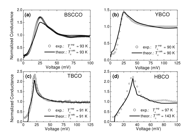
Figure 11: Comparison of the theoretical normalized tunneling conductance curves to the experimental data obtained on BSCCO (a) PhysC97 , YBCO (b) YBCO , TBCO (c) TBCO , HBCO (d) HBCO . The symmetry of the order parameter used in the calculations is $d$-wave in cases (a) and (b), and $s$+i$d$-wave in cases (c) and (d). For details on the values of the parameters see Table II.

In the cases of BSCCO and YBCO the theoretical curves follow well the behaviour of experimental data, and also the calculated $T_{\mathrm{c}}$ agrees with the measured one. In both these cases, due to the low zero-bias anomaly ($\approx\,$0.2), the best result is obtained with a very small impurity content ($\Gamma=0.5$ meV and $\Gamma=0.6$ meV, respectively). The zero-bias has approximately the same value also in the cases of TBCO (0.19) and HBCO (0.23). However, in these cases the best agreement is obtained with $\Gamma$ = 0, because in the presence of impurities the peak of the theoretical curve results too low with respect to the experimental one. It is easily seen that the agreement is better for TBCO than for HBCO. In this latter case, to obtain an acceptable result we were forced to use parameters that give a calculated critical temperature $T_{\mathrm{c}}^{\mathrm{calc}}=143$ K which is much greater than the measured one ($T_{\mathrm{c}}^{\mathrm{exp}}=97$ K), while in all the other cases $T_{\mathrm{c}}^{\mathrm{calc}}\approx T_{\mathrm{c}}^{\mathrm{exp}}$.

Let us conclude with a brief discussion of the assumption $\mu^{\ast}=0$ we made at the beginning of this paper. This simplifying assumption could appear poorly adequate to describe the HTSC, where the Coulomb pseudopotential is, as well known, different from zero. Actually, the main effect of each component of $\mu^{*}$ (isotropic and anisotropic) is to change the scale of the corresponding coupling strength. Then, almost the same tunneling curves can be obtained with $\mu^{*}=0$ and given values of the coupling constants, let’s say $\lambda_{\rm is}^{(1)}$ and $\lambda_{\rm an}^{(1)}$, or with $\mu^{*}_{\rm is}$ and $\mu^{*}_{\rm an}$ different from zero and coupling constants $\lambda_{\rm is}^{(2)}>\lambda_{\rm is}^{(1)}$ and $\lambda_{\rm an}^{(2)}>\lambda_{\rm an}^{(1)}$.

V Conclusions

We calculated the theoretical normalized tunneling conductance of SIN junctions for six different symmetries of the superconducting order parameter, by solving the real-axis EEs both in the presence and in the absence of scattering from non-magnetic impurities. We demonstrated that, in spite of being a much more complicated and time-consuming procedure, this approach is preferable to the analytical continuation of the solution of the imaginary-axis EEs, especially if a comparison of the theoretical predictions with good experimental data is required.

For each of the symmetries considered, we also studied the temperature dependence of the tunneling conductance curves, showing that at the increase of temperature the information about the pairing symmetry is progressively lost.

Finally, we discussed an example of how our calculations can be applied to a physical system, by comparing the theoretical curves to experimental tunneling data obtained on BSCCO, YBCO, TBCO and HBCO. Of course, it must be borne in mind that the applicability of the Eliashberg theory to these materials is controversial, and the reliability of the results is limited by the very complex phenomenology of high-$T_{\rm c}$ superconductors.

Unexpectedly, the results of such a comparison are fairly good. The theoretical curves reproduce some of the unusual properties of the tunneling curves of HTSC: the high $T_{\rm c}$, the broadening of the conductance peak, the conductance excess below the gap, the zero bias and also the presence of a ‘dip’ and a ‘hump’ at 2$\Delta/e$ and $3\Delta/e$, respectively. The results also seem to confirm, for these materials, the plausibility of a $d$-wave gap symmetry, or at least of a dominant $d$-wave component of the order parameter.

Even though alternative approaches to high-$T_{\rm c}$ superconductivity are nowadays preferred, maybe all these results indicate that, as far as the tunneling conductance is concerned, the Eliashberg theory mimics a (still unknown) theory of high-$T_{\rm c}$ superconductivity, whose mechanism could at least partially differ from the electron-boson coupling.

References

- (1) G.M. Eliashberg, Sov. Phys. JETP 3, 696 (1963).
- (2) D.J. Van Harlingen, Rev. Mod. Phys. 67, 515 (1995).
- (3) J.P. Carbotte, Rev. Mod. Phys. 62, 1028 (1990) .
- (4) P.B. Allen and B. Mitrovich, in Solid State Physics, Vol. 37 (Academic Press, New York, 1982).
- (5) C.T. Rieck, D. Fay and L. Tewordt, Phys. Rev. B 41, 7289 (1989) .
- (6) G. Strinati and U. Fano, Journal of Mathematical Physics 17, 434 (1976); P.B. Allen, Lect. Notes Phys. 115, 388 (1980).
- (7) C. Jiang and J.P. Carbotte, Phys. Rev. B 57, 3045 (1998); 53, 12400 (1996); 45, 7368 (1992); C. Jiang, J.P. Carbotte and R.C. Dynes, ibid. 47, 5325 (1993); E. Schachinger, J.P. Carbotte and F. Marsiglio, ibid. 47, 5325 (1993); G.A. Ummarino, R.S. Gonnelli and D. Daghero, Physica C 341-348 (2000) 299.
- (8) K.A. Musaelian, J. Betouras, A.V. Chubukov and R. Joynt, Phys. Rev. B 53, 3598 (1996).
- (9) G.A. Ummarino and R.S. Gonnelli, Physica C 328, 189 (1999).
- (10) C. Jiang, J.P. Carbotte and R.C. Dynes, Phys. Rev. B 47, 5325 (1993).
- (11) O.V. Dolgov and A.A. Golubov, Int. J. Mod. Phys. B 1, 1089 (1988).
- (12) S. Kashiwaya and Y. Tanaka, Rep. Prog. Phys. 63, 1641 (2000).
- (13) H.J. Vidberg, J.W. Serene, J. Low Temp. Phys. 29, 179 (1977).
- (14) G. Varelogiannis, Physica C 51, 1381 (1995).
- (15) R.S. Gonnelli, G.A. Ummarino and V.A. Stepanov, Physica C 275, 162 (1997).
- (16) G.A. Ummarino and R.S. Gonnelli, Physica C 341-348, 295 (2000).
- (17) G. Varelogiannis, Phys. Rev. B 51, 1381 (1995).
- (18) L. Ozyuzer, J.F. Zasadzinski, N. Miyakawa, C. Kendziora and K.E. Gray, Phys. Rev. B 61, 3629 (2000); J.F. Zasadzinski, L. Ozyuzer, N. Miyakawa, D.G. Hinks and K.E. Gray, Physica C 341-348, 867 (2000); N. Miyakawa, J.F. Zasadzinski, L. Ozyuzer, P.Guptasarma, C.Kendziora, D.G. Hinks, T.Kaneko and K.E. Gray, Physica C 341-348, 835 (2000).
- (19) Ar. Abanov, A.V. Chubukov, Phys. Rev. B 61 R9241 (2000).
- (20) R. Combescot, Phys. Rev. B 51 11625 (1995); R. Combescot, O.V. Dolgov, D. Rainer, S.V. Shulga, Phys. Rev. B 53 2739 (1996).
- (21) A.M. Cucolo, R. Di Leo, A. Nigro, P. Romano, F. Bobba, E. Bacca, P. Prieto, Phys. Rev. Lett. 76, 7810 (1996).
- (22) L. Ozyuzer, J.F. Zasadzinski, C. Kendziora, K.E. Gray, Phys. Rev. B 57, 3245 (1998).
- (23) J.Y.T. Wei, C.C. Tsuei, P.J.M. van Bentum, Q. Xiong, C.W. Chu, M.K. Wu, Phys. Rev. B 57, 3650 (1998).
- (24) M. Arai, K. Yamada, S. Hosoya, S. Wakimoto, T. Otomo, K. Ubukata, M. Fujita, T. Nishijima, Y. Endoh, Physica C 235-240, 1253 (1994); Prafulla K. Jha, Sankar P. Sanyal, ibid. 271, 6 (1996); W. Reichardt, D. Ewert, E. Gering, F. Gompf, L. Pintschovius, B. Renker, G. Collin, A.J. Dianoux, H. Mutka, Physica B 156-157, 897 (1989); S.L. Chaplot, B.A. Dasannacharya R. Mukhopadhyay, K.R. Rao, P.R. Vijayaraghavan, R.M. Iyer, G.M. Phaak, J.V. Yakhmi, ibid. 174, 378 (1991).
- (25) H. Hancotte, R. Deltour, D.N. Davydov, A.G.M Jansen and P. Wyder, Phys. Rev. B 55, R3410 (1998).
- (26) Y. DeWilde, N. Miyakawa, P. Guptasarma, M. Iavarone, L. Ozyuzer, J.F. Zasadzinski, P. Romano, D.G. Hinks, C. Kenziora, G.W. Crabtree and K.E. Gray, Phys. Rev. Lett. 80, 153 (1998).
- (27) Ch. Renner, B. Revaz, J.-Y. Genoud, K. Kadowaki and Ø. Fischer, Phys. Rev. Lett. 80, 149 (1998).
- (28) S.H. Pan, E.W. Hudson, K.M. Lang, H. Eisaki, S. Uchida and J.C. Davis, Nature 403, 746 (2000).
- (29) R.S. Gonnelli, G.A. Ummarino and V.A. Stepanov, Physica C 317-318, 378 (1999).
- (30) R.S. Gonnelli, G.A. Ummarino, D. Daghero, L. Natale, A. Calzolari, V.A. Stepanov, M. Ferretti, Int. J. Mod. Phys. B, 14, 3472 (2000).