Ab Initio Treatments of the Ising Model in a Transverse Field

Abstract

In this article, new results are presented for the zero-temperature ground-state properties of the spin-half transverse Ising model on various lattices using three different approximate techniques. These are, respectively, the coupled cluster method, the correlated basis function method, and the variational quantum Monte Carlo method. The methods, at different levels of approximation, are used to study the ground-state properties of these systems, and the results are found to be in excellent agreement both with each other and with results of exact calculations for the linear chain and results of exact cumulant series expansions for lattices of higher spatial dimension. The different techniques used are compared and contrasted in the light of these results, and the constructions of the approximate ground-state wave functions are especially discussed.

I Introduction

Two of the most versatile and most accurate semi-analytical formalisms of microscopic quantum many-body theory (QMBT) are the coupled cluster method theory_ccm1 ; theory_ccm2 ; theory_ccm3 ; theory_ccm4 ; theory_ccm5 ; theory_ccm6 ; theory_ccm7 ; theory_ccm8 and the correlated basis function (CBF) method theory_cbf1 ; theory_cbf2 ; theory_cbf3 ; theory_cbf4 ; theory_cbf5 ; theory_cbf6 ; theory_cbf7 ; theory_cbf8 ; theory_cbf9 ; theory_cbf10 ; theory_cbf11 . In recent years such QMBT methods, together with various quantum Monte Carlo (QMC) techniques, have been applied with a great deal of success to lattice quantum spin systems at zero temperature. Some typical recent examples of such applications include Refs. ccm3 ; ccm8 ; ccm16 ; ccm18 ; ccm19 ; ccm20 ; ccm21 ; ccm22 for the CCM, Refs. cbf1 ; cbf2 ; cbf3 ; cbf4 for the CBF method, and Refs. qmc1 ; qmc2 ; qmc3 ; qmc4 ; qmc5 ; qmc6 ; qmc7 ; qmc8 for the various QMC techniques. Current state of the art is such that these methods are sufficiently accurate to describe the various quantum phase transitions between the states of different quantum order that exist in such abundance for spin-lattice systems. However, each of the above methods is characterised by its own strengths and weaknesses. Hence, a fuller and more complete understanding of such strongly interacting systems as the lattice quantum spin systems is expected to be given by the application of a range of such techniques than by the single application of any one of them. In this article we wish to apply the CCM, the CBF method, and the variational quantum Monte Carlo (VQMC) method to the spin-half transverse Ising model (for reviews of this model see, for example, Refs. new_ref1 ; new_ref2 ; new_ref3 ; new_ref4 ; new_ref5 ; exact_1D ). The Hamiltonian for this model on a lattice of $N$ sites, each of which has $z$ nearest-neighbours, is given by

$$H=\biggl{(}\frac{z}{2}+\lambda\biggr{)}N-\sum_{\langle i,j\rangle}\sigma_{i}^{z}\sigma_{j}^{z}-\lambda\sum_{i}\sigma_{i}^{x}~{}~{},$$ (1)

where the $\sigma$-operators are the usual Pauli spin operators and $\langle i,j\rangle$ indicates that each of the $zN/2$ nearest-neighbour bonds on the lattice is counted once only. We work in the thermodynamic limit where $N\rightarrow\infty$. We note that this model has an exact solution in one dimensionexact_1D ; and approximate techniques, such as the random phase approximation (RPA) rpa and exact cumulant series expansionsseries1 ; series2 , have also been applied to it for lattices of higher spatial dimensionality. For $\lambda\geq 0$, we note furthermore that the model contains two distinct phases, with a critical coupling strength $\lambda_{c}$ depending on lattice type and dimensionality. For $\lambda<\lambda_{c}$ there is non-zero spin ordering in the $z$-direction, and hence this regime will be referred to here as the ferromagnetic regime. By contrast, for $\lambda>\lambda_{c}$, all of the ferromagnetic ordering is destroyed, and the classical behaviour of these systems is that the spins lie along the positive $x$-axis. Hence, the $\lambda>\lambda_{c}$ regime will be referred to here as the paramagnetic regime. In Sec. II the technical aspects of applying the CCM, the CBF, and the VQMC methods to the spin-half transverse Ising model are presented, and in Sec. III the results of these calculations are discussed. Finally, the conclusions are given in Sec. IV.

II Quantum Many-Body Techniques

II.1 The Coupled Cluster Method (CCM)

In this section, we firstly describe the general CCM formalism theory_ccm1 ; theory_ccm2 ; theory_ccm3 ; theory_ccm4 ; theory_ccm5 ; theory_ccm6 ; theory_ccm7 ; theory_ccm8 , and then proceed to apply it to the specific case of the spin-half transverse Ising model. The exact ket and bra ground-state energy eigenvectors, $|\Psi\rangle$ and $\langle\tilde{\Psi}|$, of a many-body system described by a Hamiltonian $H$,

$$H|\Psi\rangle=E_{g}|\Psi\rangle\;;\;\;\;\langle\tilde{\Psi}|H=E_{g}\langle\tilde{\Psi}|\;,$$ (2)

are parametrised within the single-reference CCM as follows:

$$|\Psi\rangle={\rm e}^{S}|\Phi\rangle\; \;\;\;S=\sum_{I\neq 0}{\cal S}_{I}C_{I}^{+}\;,$$ ;

$$\langle\tilde{\Psi}|=\langle\Phi|\tilde{S}{\rm e}^{-S}\; \;\;\;\tilde{S}=1+\sum_{I\neq 0}\tilde{{\cal S}}_{I}C_{I}^{-}\;.$$ ; (3)

The single model or reference state $|\Phi\rangle$ is required to have the property of being a cyclic vector with respect to two well-defined Abelian subalgebras of multi-configurational creation operators $\{C_{I}^{+}\}$ and their Hermitian-adjoint destruction counterparts $\{C_{I}^{-}\equiv(C_{I}^{+})^{\dagger}\}$. Thus, $|\Phi\rangle$ plays the role of a vacuum state with respect to a suitable set of (mutually commuting) many-body creation operators $\{C_{I}^{+}\}$,

$$C_{I}^{-}|\Phi\rangle=0\;\;,\;\;\;I\neq 0\;,$$ (4)

with $C_{0}^{-}\equiv 1$, the identity operator. These operators are complete in the many-body Hilbert (or Fock) space,

$$1=|\Phi\rangle\langle\Phi|+\sum_{I\neq 0}C_{I}^{+}|\Phi\rangle\langle\Phi|C_{I}^{-}\;.$$ (5)

Also, the correlation operator $S$ is decomposed entirely in terms of these creation operators $\{C_{I}^{+}\}$, which, when acting on the model state ($\{C_{I}^{+}|\Phi\rangle\}$), create excitations from it. We note that although the manifest Hermiticity, ($\langle\tilde{\Psi}|^{\dagger}=|\Psi\rangle/\langle\Psi|\Psi\rangle$), is lost, the intermediate normalisation condition $\langle\tilde{\Psi}|\Psi\rangle=\langle\Phi|\Psi\rangle=\langle\Phi|\Phi\rangle\equiv 1$ is explicitly imposed. The correlation coefficients $\{{\cal S}_{I},\tilde{{\cal S}}_{I}\}$ are regarded as being independent variables, even though formally we have the relation,

$$\langle\Phi|\tilde{S}=\frac{\langle\Phi|{\rm e}^{S^{\dagger}}{\rm e}^{S}}{\langle\Phi|{\rm e}^{S^{\dagger}}{\rm e}^{S}|\Phi\rangle}\;.$$ (6)

The full set $\{{\cal S}_{I},\tilde{{\cal S}}_{I}\}$ thus provides a complete description of the ground state. For instance, an arbitrary operator $A$ will have a ground-state expectation value given as,

$$\bar{A}\equiv\langle\tilde{\Psi}|A|\Psi\rangle=\langle\Phi|\tilde{S}{\rm e}^{-S}A{\rm e}^{S}|\Phi\rangle=\bar{A}\left(\{{\cal S}_{I},\tilde{{\cal S}}_{I}\}\right)\;.$$ (7)

We note that the exponentiated form of the ground-state CCM parametrisation of Eq. (3) ensures the correct counting of the independent and excited correlated many-body clusters with respect to $|\Phi\rangle$ which are present in the exact ground state $|\Psi\rangle$. It also ensures the exact incorporation of the Goldstone linked-cluster theorem, which itself guarantees the size-extensivity of all relevant extensive physical quantities.

The determination of the correlation coefficients $\{{\cal S}_{I},\tilde{{\cal S}}_{I}\}$ is achieved by taking appropriate projections onto the ground-state Schrödinger equations of Eq. (2). Equivalently, they may be determined variationally by requiring the ground-state energy expectation functional $\bar{H}(\{{\cal S}_{I},\tilde{{\cal S}}_{I}\})$, defined as in Eq. (7), to be stationary with respect to variations in each of the (independent) variables of the full set. We thereby easily derive the following coupled set of equations,

$$\delta{\bar{H}}/\delta{\tilde{{\cal S}}_{I}}=0 \Rightarrow \langle\Phi|C_{I}^{-}{\rm e}^{-S}H{\rm e}^{S}|\Phi\rangle=0,\;\;I\neq 0\;\;;$$ (8)

$$\delta{\bar{H}}/\delta{{\cal S}_{I}}=0 \Rightarrow \langle\Phi|\tilde{S}{\rm e}^{-S}[H,C_{I}^{+}]{\rm e}^{S}|\Phi\rangle=0,\;\;I\neq 0\;\;.$$ (9)

Equation (8) also shows that the ground-state energy at the stationary point has the simple form

$$E_{g}=E_{g}(\{{\cal S}_{I}\})=\langle\Phi|{\rm e}^{-S}H{\rm e}^{S}|\Phi\rangle\;\;.$$ (10)

It is important to realize that this (bi-)variational formulation does not lead to an upper bound for $E_{g}$ when the summations for $S$ and $\tilde{S}$ in Eq. (3) are truncated, due to the lack of exact Hermiticity when such approximations are made. However, it is clear that the important Hellmann-Feynman theorem is preserved in all such approximations.

We also note that Eq. (8) represents a coupled set of nonlinear multinomial equations for the c-number correlation coefficients $\{{\cal S}_{I}\}$. The nested commutator expansion of the similarity-transformed Hamiltonian,

$$\hat{H}\equiv{\rm e}^{-S}H{\rm e}^{S}=H+[H,S]+{1\over 2!}[[H,S],S]+\cdots\;\;,$$ (11)

together with the fact that all of the individual components of $S$ in the sum in Eq. (3) commute with one another, imply that each element of $S$ in Eq. (3) is linked directly to the Hamiltonian in each of the terms in Eq. (11). Thus, each of the coupled equations (8) is of linked cluster type. Furthermore, each of these equations is of finite length when expanded, since the otherwise infinite series of Eq. (11) will always terminate at a finite order, provided (as is usually the case) that each term in the second-quantised form of the Hamiltonian $H$ contains a finite number of single-body destruction operators, defined with respect to the reference (vacuum) state $|\Phi\rangle$. Therefore, the CCM parametrisation naturally leads to a workable scheme which can be efficiently implemented computationally. It is also important to note that at the heart of the CCM lies a similarity transformation, in contrast with the unitary transformation in a standard variational formulation in which the bra state $\langle\tilde{\Psi}|$ is simply taken as the explicit Hermitian adjoint of $|\Psi\rangle$.

The CCM formalism is exact in the limit of inclusion of all possible multi-spin cluster correlations for $S$ and $\tilde{S}$, although in any real application this is usually impossible to achieve. It is therefore necessary to utilise various approximation schemes within $S$ and $\tilde{S}$. The three most commonly employed schemes previously utilised have been: (1) the SUB$n$ scheme, in which all correlations involving only $n$ or fewer spins are retained, but no further restriction is made concerning their spatial separation on the lattice; (2) the SUB$n$-$m$ sub-approximation, in which all SUB$n$ correlations spanning a range of no more than $m$ adjacent lattice sites are retained; and (3) the localised LSUB$m$ scheme, in which all multi-spin correlations over distinct locales on the lattice defined by $m$ or fewer contiguous sites are retained. The specific application of the CCM to the spin-half transverse Ising model in the paramagnetic and ferromagnetic regimes is now described.

II.1.1 The Paramagnetic Regime

In the paramagnetic regime, a model state is utilised in which all spins point along the $x$-axis, although it is found to be useful to rotate the local spin coordinates of these spins such that all spins in the model state point in the ‘downwards’ direction (i.e., along the negative $z$-axis). This (canonical) transformation is given by,

$$\sigma^{x}\rightarrow-\sigma^{z}~{}~{},~{}~{}\sigma^{y}\rightarrow\sigma^{y}~{}~{},~{}~{}\sigma^{z}\rightarrow\sigma^{x}~{}~{},$$ (12)

such that the transverse Ising Hamiltonian of Eq. (1) is now given in the (rotated) spin-coordinate frame by,

$$H=\biggl{(}\frac{z}{2}+\lambda\biggr{)}N-\sum_{\langle i,j\rangle}\biggl{[}\sigma_{i}^{+}\sigma_{j}^{+}+\sigma_{i}^{-}\sigma_{j}^{-}+\sigma_{i}^{-}\sigma_{j}^{+}+\sigma_{i}^{+}\sigma_{j}^{-}\biggr{]}+\lambda\sum_{i}\sigma_{i}^{z}~{}~{},$$ (13)

where $\sigma_{k}^{\pm}\equiv\frac{1}{2}(\sigma_{k}^{x}\pm{\rm i}\sigma_{k}^{y})$. In these local coordinates the model state is thus the “ferromagnetic” state $|\Psi\rangle=|~{}\downarrow\downarrow\cdots\downarrow\cdots\rangle$ in which all spins point in the downwards direction. In order to reflect the symmetries of this Hamiltonian, the cluster correlations within $S$ are explicitly restricted to those for which $s_{T}^{z}=\sum_{i}s_{i}^{z}$ (in the rotated coordinate frame) is an even number. Hence, the LSUB2 approximation is defined by

$$S=\frac{b_{1}}{2}~{}\sum_{i,\rho}\sigma_{i}^{+}\sigma_{i+\rho}^{+}~{}~{},$$ (14)

where $\rho$ covers all nearest-neighbour lattice vectors. The ground-state energy is now given in terms of $b_{1}$ by,

$$\frac{E}{N}=\frac{z}{2}(1-b_{1})~{}~{}.$$ (15)

It is found that this expression is valid for any level of approximation for $S$. Using Eq. (7) it is found that,

$$5b_{1}^{2}+4\lambda b_{1}-1=0~{}~{},$$ (16)

and hence an approximate solution for the ground-state energy at the LSUB2 approximation level purely in terms of $\lambda$ may be obtained. The SUB2 approximation contains all possible two-body correlations, for a given lattice, and is defined by

$$S=\frac{1}{2}\sum_{i}\sum_{r}b_{r}~{}\sigma_{i}^{+}\sigma_{i+r}^{+}~{}~{},$$ (17)

where the index $r$ indicates a lattice vector. Eq. (7) may once again be utilised to determine the SUB2 ket-state equations. Hence the CCM SUB2 ket-state equation corresponding to a two-body correlation characterised by index $s$ is given by,

$$(1+2b_{1}^{2})\delta_{s,\rho}-4b_{1}b_{s}+\sum_{r}b_{r}b_{r+s+\rho}+2b_{s+\rho}-4\lambda b_{s} = 0~{}~{}.$$ (18)

We note that this equation is meaningful only for $s\neq 0$ as we may only ever have one Pauli raising operator per lattice site. This equation may be solved by performing a Fourier transformation. (Details of how this is achieved in practice are not given here and the interested reader is referred to Refs. ccm3 ; ccm18 .) An alternative approach, however, is to use Eq. (18) in order to fully define the SUB2-$m$ equations. This is achieved by truncating the range of the two-body correlations (i.e., by setting $|s|\leq m$), and the corresponding SUB2-$m$ equations may be solved numerically via the Newton-Raphson technique (or other such techniques). We note that coupled sets of high-order LSUB$m$ equations may be derived using computer-algebraic techniques, as discussed in Ref. ccm19 . The technicalities of these calculations are not considered here, but the interested reader is referred to Ref. ccm19 . A full discussion of the CCM results based on the paramagnetic model state is deferred until Sec. III.

II.1.2 The Ferromagnetic Regime

In the ferromagnetic regime, a model state is chosen in which all spins point ‘downwards’ (along the negative $z$-axis), and so the Hamiltonian of Eq. (1) may therefore be utilised directly within the CCM calculations. The lowest order approximation is the now SUB1 approximation (in which case, $S=a\sum_{i}\sigma_{i}^{+}$) and the ground-state energy is given in terms of $a$ by,

$$\frac{E}{N}=\lambda(1-a)~{}~{}.$$ (19)

It is again noted that this expression is valid for any level of approximation in $S$. In this case, it is found that the solution of the SUB2 approximation collapses onto the LSUB2 solution due to the simple nature of the Hamiltonian and model state, although it is again possible to perform high-order LSUB$m$ calculations. Furthermore, the lattice magnetisation (i.e., the magnetisation in the $z$-direction), $M$, is defined within the CCM framework by,

$$M=-\frac{1}{N}\sum_{i=1}^{N}\langle\tilde{\Psi}\mid\sigma_{i}^{z}\mid\Psi\rangle~{}~{},$$ (20)

which may be determined once both the ket- and bra-state equations have been solved at a given level of approximation. Again, the discussion of the results for this model state is deferred until Section III.

II.2 The CBF Formalism

The treatment of the transverse Ising model by the CBF method is begun by defining the lattice magnetisation (i.e., again the magnetisation in the $z$-direction), given by

$$M=\frac{\langle\psi\mid\sigma_{i}^{z}\mid\psi\rangle}{\langle\psi|\psi\rangle}~{}~{},$$ (21)

for a ground-state trial wave function, $|\psi\rangle$. Furthermore, the ‘transverse’ magnetisation is given by,

$$A=\frac{\langle\psi\mid\sigma_{i}^{x}\mid\psi\rangle}{\langle\psi|\psi\rangle}~{}~{}.$$ (22)

It is also found to be useful to define a spatial distribution function (which plays a crucial part in any CBF calculation) in the following manner,

$$g({\bf n})=\frac{\langle\psi\mid\sigma_{i}^{z}\sigma_{j}^{z}\mid\psi\rangle}{\langle\psi|\psi\rangle}~{}~{},$$ (23)

where ${\bf n}={\bf r}_{i}-{\bf r}_{j}$. The corresponding approximation to the ground-state energy per spin is given by

$$\frac{E}{N}=\frac{\langle\psi|H|\psi\rangle}{N\langle\psi|\psi\rangle}=\frac{z}{2}-\sum_{{\bf n}}\Delta({\bf n})g({\bf n})+\lambda(1-A)~{}~{},$$ (24)

where the function $\Delta({\bf n})$ is equal to unity when ${\bf n}$ is a nearest-neighbour lattice vector and is zero elsewhere. It is noted that the distribution function $g({\bf n})$ may be decomposed according to $g({\bf n})=\delta_{{{\bf n}},0}+(1-\delta_{{{\bf n}},0})M^{2}+(1-M^{2})G({\bf n})$ such that $G({\bf n})$ now contains the short-range part of the spatial distribution function and vanishes in the limit $|{\bf n}|\rightarrow\infty$. The magnetisation, $M$, and the transverse magnetisation, $A$, may now be expressed in a factorised form in terms of a ‘spin-exchange strength’, $n_{12}$, such that,

$$A=(1-M^{2})^{\frac{1}{2}}n_{12}~{}~{}.$$ (25)

The energy functional is now expressed in terms of $G({\bf n})$ and $n_{12}$ as,

$$\frac{E}{N}=(1-M^{2})\biggl{\{}\frac{z}{2}-\sum_{{\bf n}}\Delta({\bf n})G({\bf n})\biggr{\}}+\lambda\biggl{\{}1-(1-M^{2})^{\frac{1}{2}}n_{12}\biggr{\}}~{}~{}.$$ (26)

Note that in the mean-field approximation $G({\bf n})$ in Eq. (26) is set to zero (for all ${\bf n}$) and $n_{12}$ is set to unity.

In order to determine the ground-state energy and other such ground-state expectation values, a Hartree-Jastrow Ansatz is now introduced, given by

$$|\psi\rangle={\rm exp}\{MU_{M}+U\}|0\rangle~{}~{}.$$ (27)

The reference state $|0\rangle$ is a tensor product of spin states which have eigenvalues of $+1$ with respect to $\sigma^{x}$. The correlation operators $U$ and $U_{M}$ are written in terms of pseudopotentials, $u({\bf r}_{ij})$, $u_{1}({\bf r}_{i})$, and $u_{M}({\bf r}_{ij})$, where

$$U=\frac{1}{2}\sum_{i<j}^{N}u({\bf r}_{ij})\sigma_{i}^{z}\sigma_{j}^{z}~{}~{},$$ (28)

and

$$U_{M}=\sum_{i}^{N}u_{1}({\bf r}_{i})\sigma_{i}^{z}+\frac{1}{4}\sum_{i<j}^{N}u_{M}({\bf r}_{ij})(\sigma_{i}^{z}+\sigma_{j}^{z})~{}~{}.$$ (29)

The pseudopotential $u_{1}({\bf r}_{i})\equiv u_{1}$ is independent of the lattice position by translational invariance, and the pseudopotentials, $u({\bf r}_{ij})$ and $u_{M}({\bf r}_{ij})$, similarly depend only on the relative distance, $|{\bf n}|=|{\bf r}_{i}-{\bf r}_{j}|\equiv|{\bf r}_{ij}|$. The Jastrow correlations are determined via a cluster expansion of the various quantities in the Hamiltonian, as explained in Refs. cbf1 ; cbf2 ; cbf3 ; cbf4 . A common approximation yields the hypernetted chain (HNC/0) equations, which one may solve iteratively in order to determine the Hartree-Jastrow pseudopotentials. One then wishes to determine the expectation values such as the ground-state energy, and in the paramagnetic regime an explicit assumption is made that $M=0$. However, in the ferromagnetic regime $M$ is taken to be a variational parameter with respect to the ground-state energy of Eq. (26).

There are now two ways of determining the pseudopotentials from the HNC equations. The first such approach is to assume that the pseudopotential has the simple parametrised form,

$$u({\bf n})=\alpha~{}\Delta({\bf n})~{}~{},$$ (30)

where $\Delta({\bf n})$ is unity if ${\bf n}$ is a nearest-neighbour lattice vector and is zero otherwise. This approach is henceforth denoted as the parametrised HNC CBF method. The $c$-number $\alpha$ is taken to be a variational parameter with respect to which the ground-state energy is minimized. In the paramagnetic regime, the minimum of the energy surface as a function of $\alpha$ is sought, at a given value of $\lambda$. This is easily performed computationally, and the solution is readily tracked iteratively, starting from the trivial limit $\lambda\rightarrow\infty$ and then moving to smaller values of $\lambda$. In the ferromagnetic regime, one again searches for a minimum of the energy surface, but this time with respect to both $\alpha$ and $M$, at a given value of $\lambda$. In this case, one tracks from the trivial limit of $\lambda=0$ to higher values of $\lambda$. In previous articlescbf1 ; cbf2 ; cbf3 ; cbf4 , this was achieved by analytically determining the derivative of the energy with respect to $M$, although in this article a computational minimisation of the energy is performed with respect to both variables. The second such approach allows one to find the optimal pseudopotential within the CBF/HNC framework from a functional minimisation,

$$\frac{\delta E}{\delta u({\bf n})}=0~{}~{}.$$ (31)

Within the context of this article, this is henceforth denoted as the paired phonon approximation (PPA) (or, more precisely, the paired magnon approximation), and the corresponding equations are the PPA equations. Note that in this article the PPA calculation is only performed in the paramagnetic regime, although PPA results in the ferromagnetic regime have also been performed previouslycbf2 ; cbf3 . (Indeed, results for the phase transition points predicted by the PPA CBF approach of Ref.cbf2 ; cbf3 are quoted in the Table 1.) A full discussion of the results of the CBF calculations presented in this section, in comparison to the corresponding results of the CCM and the VQMC method, is given in Section III.

II.3 The VQMC Formalism

Although the specific variational calculations presented in this article concentrate on the spin-half transverse Ising model, we note that the formalism presented in this section is given in a generalised form and that the treatment of other spin models would follow a similar pattern. We shall specifically consider here the transverse Ising model in the ferromagnetic regime where the relevant Hamiltonian is defined by Eq. (1). An Ansatz for the expansion coefficients, $\{c_{I}\}$, of a ground-state wave function defined by

$$|\psi\rangle=\sum_{I}c_{I}|I\rangle~{}~{},$$ (32)

is chosen. Note that $\{|I\rangle\}$ denotes a complete set of Ising basis states, defined as all possible tensor products of states on all sites having eigenvalues $\pm 1$ with respect to $\sigma^{z}$. An expression for the ground-state energy is thus given by,

$$E=\frac{\sum_{I_{1},I_{2}}c_{I_{1}}^{*}c_{I_{2}}\langle I_{1}|H|I_{2}\rangle}{\sum_{I^{\prime}}|c_{I^{\prime}}|^{2}}~{}~{}.$$ (33)

Specifically for the spin-half transverse Ising model, a Hartree-Jastrow Ansatz variational_1D (for $\lambda>0$) is now defined with respect to the $\{c_{I}\}$ expansion coefficients, where

$$c_{I}=\langle I|\prod_{k}\biggl{(}1+a_{k}P_{k}^{\uparrow}\biggr{)}\prod_{i<j}\biggl{(}1+f_{i,j}\biggl{[}P_{i}^{\uparrow}P_{j}^{\downarrow}+P_{i}^{\downarrow}P_{j}^{\uparrow}\biggr{]}\biggr{)}|I\rangle~{}~{}.$$ (34)

The $P^{\uparrow}$ and $P^{\downarrow}$ are the usual projection operators of the spin-half ‘up’ and ‘down’ states respectively. The simplest form of the variational Ansatz of Eq. (34) is given by,

$$f_{i,j}=~{}~{}~{}\left\{~{}~{}~{}\mbox{ \begin{tabular}[]{ll}$f_{1}$&if $i$ and $j$ are nearest neighbours,\\ 0&otherwise.\end{tabular} }\right.$$ (35)

The symmetry-breaking term $a_{k}(=a)$ is also independent of $i$ by translational invariance. The expectation value of Eq. (33) may now be evaluated directly and the variational ground-state energy minimised with respect to both $a$ and $f_{1}$ at each value of $\lambda$. However, such a calculation is soon limited by the rapidly increasing set of Ising states and the amount of computational power available. Indeed, for the spin-half transverse Ising model the number of states that one must sum over is $2^{N}$, where $N$ is the number of lattice sites. For the linear chain it is possible to solve for chains of length $N\stackrel{{\scriptstyle<}}{{\sim}}12$ with relatively little computational difficulty, although the calculations with $N>12$ grow rapidly in computational difficulty.

Hence, as an alternative for lattices of larger size, we may simulate the summation over all the states $I_{1}$ in Eq. (33). In order to to do this we define the probability distribution for the set of states $\{|I\rangle\}$, given by

$$P(I)\equiv\frac{|c_{I}|^{2}}{\sum_{I^{\prime}}|c_{I^{\prime}}|^{2}}~{}~{},$$ (36)

and the local energy of these states, given by

$$E_{L}(I)\equiv\sum_{I_{1}}\frac{c_{I_{1}}}{c_{I}}\langle I|H|I_{1}\rangle~{}~{}.$$ (37)

The expression of Eq. (33) may thus be equivalently written as,

$$E=\sum_{I}~{}P(I)~{}E_{L}(I)~{}~{}.$$ (38)

We now wish to perform a random walk based on the probability distribution of Eq. (36). However, a few more useful quantities are best defined before a detailed description of the VQMC algorithm is actually given. Firstly, the acceptance probability, $A(I\rightarrow I^{\prime})$, of Monte Carlo ‘move’ from state $|I\rangle$ to state $|I^{\prime}\rangle$ is given by

$$A(I\rightarrow I^{\prime})={\rm min}~{}[1,q(I\rightarrow I^{\prime})]~{}~{},$$ (39)

where

$$q(I\rightarrow I^{\prime})\equiv\frac{P(I^{\prime})T(I^{\prime}\rightarrow I)}{P(I)T(I\rightarrow I^{\prime})}~{}~{}.$$ (40)

Here, $T(I\rightarrow I^{\prime})$ is the sampling distribution function. For spin lattice problems, if state $|I\rangle$ can connect to $K(I)$ possible Ising states via the off-diagonal elements of the Hamiltonian then $T(I\rightarrow I^{\prime})=1/K(I)$. Hence, $q(I\rightarrow I^{\prime})$ is written as

$$q(I\rightarrow I^{\prime})=\frac{P(I^{\prime})K(I)}{P(I)K(I^{\prime})}~{}~{}.$$ (41)

For the spin-half transverse Ising model, we note that $K(I)$ is equal to $N$ for any state $|I\rangle$ and so the common factor of $N$ in Eq. (41) cancels. The simplest VQMC procedure is now defined by the following algorithm:

1. Select an initial Ising state $|I\rangle$ for which $\langle I|\Psi\rangle\neq 0$, where $|\Psi\rangle$ is the ‘true’ ground-state wave function of the system.

2. Choose a particular state $|I^{\prime}\rangle$ out of the $K(I)$ possible states accessible to $|I\rangle$ via the off-diagonal elements in $H$.

3. Define a random number $r$ in the range $[0,1]$ and accept this move from state $|I\rangle$ to state $|I^{\prime}\rangle$ if and only if

   $$A(I\rightarrow I^{\prime})>r~{}~{}.$$ (42)

4. If the move is accepted then let $I\rightarrow I^{\prime}$ and $c_{I}\rightarrow c_{I^{\prime}}$.

5. Obtain the local energy $E(I)$ of Eq. (37) for state $|I\rangle$.

6. Repeat from stage (2) $N_{MC}$ times.

7. The average ground-state energy (and the error therein) may be determined from the $N_{MC}$ number of local energies during the simulation.

The minimal VQMC ground-state energy is now obtained by searching over the variational parameter space for either the lowest ground-state energy or lowest variance in the ground-state energy (here for a given value of $\lambda$ in $H$). In order to determine the lattice magnetisation, we note that

$$M = \biggl{|}\frac{\langle\psi|\sum_{i}\sigma_{i}^{z}|\psi\rangle}{N\langle\psi|\psi\rangle}\biggr{|}~{}~{},$$ (43)

$$= \biggl{|}\sum_{I}P(I)M_{L}(I)\biggr{|}~{}~{},$$

where $P(I)$ is the probability density function given above, and

$$M_{L}(I)\equiv\sum_{I_{1}}\frac{c_{I_{1}}}{Nc_{I}}\langle I|\sum_{i}\sigma_{i}^{z}|I_{1}\rangle=\frac{1}{N}\langle I|\sum_{i}\sigma_{i}^{z}|I\rangle~{}~{}.$$ (44)

Hence, a mean value (and its associated error) for the VQMC lattice magnetisation, $M$, may be obtained by determining the average of the local lattice magnetisation, $M_{L}(I)$, throughout the lifetime of the run. A discussion of the results of the variational calculations discussed here is given in Section III.

II.4 The Infinite Lattice Limit and Convergence of Results

In this section we consider how the results of each method are determined in the infinite lattice limit. Firstly, it is noted that the CCM method produces expectation values which are size-extensive (i.e., the numerical values of each expectation value scale linearly with $N$), and we always deal with an infinite lattice in all calculations from the very outset. Furthermore, the ‘raw’ CCM LSUB$m$ results based on the ferromagnetic model state are found to converge rapidly with increasing LSUB$m$ approximation level $m$ over most of the ferromagnetic regime except for a region very near to the phase transition point. In order to obtain even better results for the CCM method across the whole of this regime, a simple extrapolation of the LSUB$m$ data in the limit $m\rightarrow\infty$ has also been carried out at each value of $\lambda$ separately. The results of the extrapolation using a leading-order ‘power-law’ dependence (see Appendix A for details) are denoted as Extrapolated(1) CCM results and results of a Padé approximation for $l=0$ (again, see Appendix A for details) are called Extrapolated(2) CCM results. In the paramagnetic regime, the results for the ground-state energy are found to converge extremely rapidly with LSUB$m$ approximation level over the whole of this regime and so no extrapolation of these results is necessary.

For the CBF method, although the treatment presented here is formally valid for any lattice size (including the infinite lattice case), the results presented have been obtained for finite-sized lattices. The results are found to converge extremely rapidly with increasing lattice size, and the results of the 20$\times$20 square lattice (used in the figures given below) are found to be essentially fully converged for all $\lambda$ except for a region very near to the critical point.

The results for the VQMC method presented below have been obtained for a 16$\times$16 square lattice, where the number of Monte Carlo iterations was set to 50000. As for the CBF calculations, the 16$\times$16 lattice is again expected to be large enough for the VQMC results to be essentially fully converged to the infinite lattice limit for all values of $\lambda$ except for a region near to the critical point. By comparing the results of a 10$\times$10 lattice VQMC calculation with those of a 16$\times$16 lattice it was found that this was indeed true. Furthermore, we note that for small $\lambda$ the variational minimum of the ground-state energy was found to be rather flat with respect to the variational parameters $a$ and $f_{1}$, and the ground-state energy was also highly converged with increasing lattice size. However, as the phase transition point is approached one finds that a precise evaluation of the position of the variational minimum with respect to $a$ and $f_{1}$ becomes harder to determine.

III Results

The results for the ground-state energy per spin of the spin-half transverse Ising model on the square lattice in the ferromagnetic regime are shown in Fig. 1. We see from this figure that excellent correspondence between the results of the CCM, CBF, and VQMC methods for the ground-state energy is obtained in this regime. We note, however, that the extrapolated CCM results appear to lie very slightly lower than the other two sets of results, especially near to the phase transition point. This indicates the increasing importance of higher-order correlations for the ground-state energy near to the phase transition point.

Figure 1: Results for the ground-state energy per spin, $E_{g}/N$, of the spin-half transverse Ising model on the square lattice in the ferromagnetic regime using the CCM, CBF, and VQMC approaches.

The results for the lattice magnetisation $M$ obtained using the CCM, CBF, and VQMC formalisms are shown in Fig. 2 (and also Fig. 4 in Appendix A) for the spin-half transverse Ising model on the square lattice. We note that the ‘raw’ CCM LSUB$m$ results for the lattice magnetisation do not become zero at any value of $\lambda$ for any finite value of the truncation index $m$, because all of the ferromagnetic order inherent in the model state must be destroyed in order for $M$ to be zero in this case. In practice this is a difficult thing for the CCM to achieve with this model state. However, we may see from Fig. 2 that the extrapolated CCM results are in excellent agreement with those results of the CBF and VQMC methods. In addition, it is possible to imagine other CCM model states, such as a spin-flop model state or a mean-field model state, in which the lattice magnetisation with respect to this state is not a priori fully saturated for all $\lambda$. Furthermore, we remark that a treatment of this problem with the ferromagnetic model state using the extended coupled cluster method (ECCM) theory_ccm4 ; theory_ccm5 ; theory_ccm7 ; ccm23 would present an interesting challenge.

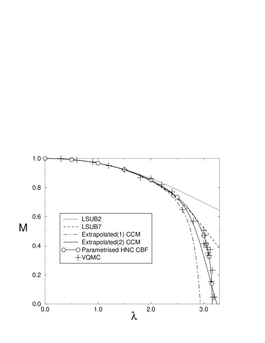
Figure 2: Results for the lattice magnetisation, $M$, of the spin-half transverse Ising model on the square lattice using the CCM, CBF, and VQMC approaches.

In the paramagnetic regime, the ground-state energy per spin for the transverse Ising model on the square lattice is presented in Fig. 3. The ‘raw’ CCM LSUB$m$ results for the ground-state energy are already highly converged with increasing truncation index $m$, even up to the phase transition point. We note again that an extrapolation in the limit $m\rightarrow\infty$ is therefore not necessary. Indeed, good correspondence between the results of the different methods is seen although it is noted that CCM LSUB4 and LSUB6 ground-state energies lie lower than those predicted by the CBF. This indicates that high-order order correlations become increasingly important the nearer one gets to the phase transition point. However, this could be rectified, in principle, for the CBF method by the inclusion of higher-order (than pairwise Jastrow) correlations in the ground-state wave function. We note that in practice, however, the inclusion of such higher-order correlations in the ground-state wave function in the CBF and VQMC methods is a difficult and unresolved question.

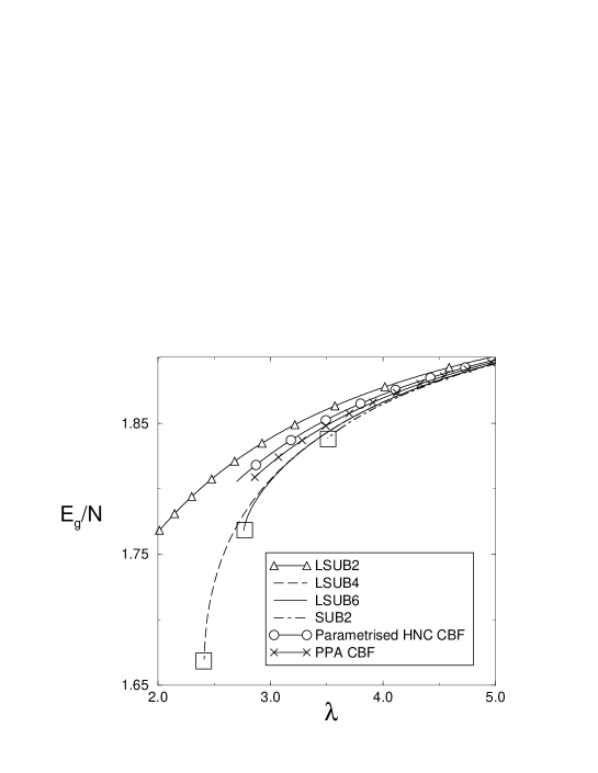
Figure 3: Results for the ground-state energy per spin, $E_{g}/N$, of the spin-half transverse Ising model on the square lattice in the paramagnetic regime using the CCM and CBF approaches. The boxes for the CCM data indicate the terminating points at which $\chi$ becomes infinite.

It is also possible to determine the second-derivative of the ground-state energy per spin with respect to $\lambda$ for the CCM calculations based on the paramagnetic model state, defined by

$$\chi\equiv-\frac{1}{N}\frac{\partial^{2}E_{g}}{\partial\lambda^{2}}~{}.$$ (45)

It is found that $\chi$ diverges at some critical value $\lambda_{c}$ for the SUB2 approximation in any dimension, and for SUB2-$m$ and LSUB$m$ (with $m\geq 4$) approximations for spatial dimensionality greater than one. Again, this behaviour is associated with a phase transition in the real system and the point at which this occurs is denoted $\lambda_{c}$. Correspondingly, CCM results for $\lambda<\lambda_{c}$ based on the paramagnetic model state do no exist, and hence $\lambda_{c}$ acts as a terminating point for the calculation in the paramagnetic regime. Also, it is found that the SUB2-$m$ results for $\lambda_{c}$ as a function of $m$ scale with $m^{-2}$ and a simple linear extrapolation gives the full SUB2 result for the critical point to within a $2\%$ accuracy. By analogy, this rule has also been used for the LSUB$m$ results to extrapolate to the limit $m\rightarrow\infty$, and the results thus determined are shown in Table 1. The values thus obtained are also in good agreement with the points at which $M\rightarrow 0$ from the extrapolations in the ferromagnetic regime discussed above (and see Fig. 2 for the square lattice case).

For the CBF and VQMC methods the point, in terms of $\lambda$, at which $M$ becomes zero is taken to indicate a quantum phase transition and is again denoted, $\lambda_{c}$, and these results are presented in Table 1. The phase transition point predicted by the VQMC method on the square lattice case is estimated to be at $\lambda_{c}=3.15\pm 0.05$. For the linear chain, the expression for ground-state energy of Eq. (33) has been obtained directly for chains with $N\leq 12$. These results are found to be in good agreement with a previous calculationvariational_1D using the Ansatz of Eq. (34) for the linear chain transverse Ising model which predicted a value for the phase transition point of $\lambda_{c}=1.206$.

Table 1: Results for the critical points of the spin-half transverse Ising model on various lattices using the CCM and CBF approaches. These results are compared to those of exact calculations for the linear chain exact_1D and to RPA rpa and exact cumulant series expansions series2 in higher spatial dimensionality. For the linear chain, we note that the LSUB$m$ approximation does not show any evidence of a critical point, at the levels of approximation shown, and this is indicated by ‘none’. (Previous CBF results of Refs. cbf1 ; cbf2 ; cbf3 for the square and cubic lattices are also appropriately indicated.)

	Linear Chain	Square	Triangular	Cubic
Classical	2	4	6	6
RPA	–	3.66	–	5.76
CCM $\lambda_{c}$ SUB2	1.44	3.51	5.42	5.55
CCM $\lambda_{c}$ LSUB4	none	2.41	4.27	3.85
CCM $\lambda_{c}$ LSUB6	none	2.76	4.57	4.61
CCM $\lambda_{c}$ LSUB$\infty$	none	3.04	4.81	5.22
parametrised HNC CBF	1.22	3.12	4.91	5.17[b]
PPA CBF	–	3.14	–	5.10
Variational or VQMC Calculations	1.206	3.15$\pm$0.05	–	–
Exact or Series Expansions Calculations	1.0	3.044	4.768[f]	5.153[f]

IV Conclusions

In this article, results of the CCM, CBF, and VQMC approaches for the ground-state energy, the lattice magnetisation, and the position of the critical point of the spin-half transverse Ising model on various lattices have been presented. These results have been seen to be in excellent agreement both with each other and with those results of exact calculations for the linear chain and those of exact cumulant series expansions for higher spatial dimensionality. Indeed, by treating these systems using three separate approaches, it has been shown that each set of results has been mutually supported and reinforced by those of the other approaches.

Furthermore, we have gained some insight into the strengths and weaknesses of each approach. This is exemplified in the different parametrisations of the ground-state wave function. The CBF and VQMC approaches both utilise Jastrow wave functions and their bra states are always the explicit Hermitian adjoints of the corresponding ket states. Hence, for the CBF and VQMC approaches, an upper bound to the true ground-state energy is, in principle, obtainable, although the approximations made in calculating the energy may destroy it. By contrast, the CCM uses a bi-variational approach in which the bra and ket states are not manifestly constrained to be Hermitian adjoints and hence an upper bound to the true ground-state energy is not necessarily obtained. Also, the CCM uses creation operators with respect to some suitably normalised model state in order to span the complete set of (here) Ising states. The other approaches, in essence, use projection operators to form the Hartree and the Jastrow correlations. For the CBF case, this is with respect to a reference state, whereas for the VQMC case, the Hartree-Jastrow Ansatz is encoded within the expansion coefficients of the ground-state wave function with respect to a complete set of Ising states. In some sense, the CCM is found to contain less correlations than the others at ‘equivalent’ levels of approximation (e.g., the CCM LSUB2 approximation versus Hartree and nearest-neighbour Jastrow correlations). A fuller account of the different parametrisations of the ground-state wave function within the CCM and CBF methods has been given in Ref. cbf4 . However, in practice the other methods are difficult to extend to approximations which contain more than two-body or three-body correlations. By contrast, the CCM is well-suited to treat such higher-order correlations via computational techniques, as has been demonstrated here. Furthermore, the CCM requires no information other than the approximation in $S$ and $\tilde{S}$ in order to determine an approximate ground state of a given system. The CBF method, however, may require that only a certain subset of all possible diagrams are summed over (e.g., the HNC/0 approximation). The VQMC approach also often requires an intimate knowledge of the manner in which the two-body correlations behave with increasing lattice separation if all two-body correlations are to be included. This information may be approximated, for example, by use of the results of spin-wave theory. In any case, it is often necessary to reduce the minimisation of the variational ground-state energy with respect to $N$ parameters to much fewer parameters. Another potential application of all of the methods presented here is the use of their ground-state wave functions as trial or guiding wave functions in (Green function or similar) quantum Monte Carlo calculations.

Finally, encouraged by these results for the transverse Ising model, we intend to extend them to other models of interest, such as systems with higher quantum spin number or those with complex crystallographic lattices. A further goal is to extend the treatment of this and other spin models, via these methods, to non-zero temperatures.

Appendix A Extrapolation of CCM Results

In this Appendix, we explain how we extrapolate a set of LSUB$m$ data points, $\{x_{i},y_{i}\}$, in the limit $i\rightarrow\infty$ at each value of some parameter ($\lambda$) within the Hamiltonian separately. Note that the number of data elements to be extrapolated is given by the index $p$. The value of $x_{i}$ is now set to be $1/m$ and $y_{i}$ is set to be the corresponding value of an expectation value (for example, the lattice magnetisation) determined using the CCM at this level of approximation at a given value of $\lambda$. Note that the value of $m$ must increase with increasing index $i$, although $m$ and $i$ do not have to be equal.

Before the extrapolation procedures are given in detail, we define some useful quantities. Firstly, the mean value of a set $\{c_{i}\}$ is denoted by $\overline{c}$ and of a set $\{d_{i}\}$ is denoted by $\overline{d}$. Secondly, the linear correlation, $R$, of a set of two-dimensional points, $\{c_{i},d_{i}\}$, is defined by

$$R\equiv\frac{\sum_{i=1}^{p}(c_{i}-\overline{c})(d_{i}-\overline{d})}{\sqrt{\sum_{i=1}^{p}(c_{i}-\overline{c})^{2}}\sqrt{\sum_{i=1}^{p}(d_{i}-\overline{d})^{2}}}~{}~{}.$$ (46)

We are now in a position to outline the the first extrapolation procedure. This procedure firstly assumes that the data scales with a leading-order “power-law” dependence, given by

$$y_{i}=a+bx_{i}^{\nu}~{}~{}.$$ (47)

We set $c_{i}={\rm log}(x_{i})$ and $d_{i}={\rm log}(y_{i}-a)$, where $\{x_{i},y_{i}\}$ is the LSUB$m$ data set at some fixed value of a parameter within the Hamiltonian. Hence the best fit of the data set, $\{x_{i},y_{i}\}$, to the power-law dependence of Eq. (47) is obtained when the absolute value of $R$ is maximised with respect to the variable $a$. Indeed, we make the assumption that this value of $a$ is then taken to be the extrapolated value of the $y_{i}$ in the limit $i\rightarrow\infty$ (in which case, $x_{i}\rightarrow 0$).

The second extrapolation procedure of the LSUB$m$ data uses Padé approximants. This is achieved by firstly assuming that the set of data can be modeled by the ratio of two polynomials, given by

$$y_{i}=\frac{\sum_{j=0}^{k}a_{j}x_{i}^{j}}{1+\sum_{j=1}^{l}b_{j}x_{i}^{j}}~{}~{}.$$ (48)

Note that when $l=0$, this is a simple integral power series. This furthermore implies that,

$$a_{0}+a_{1}x_{i}+a_{2}x_{i}^{2}+\cdots+a_{k}x_{i}^{k}=y_{i}+(b_{1}x_{i}+b_{2}x_{i}^{2}+\cdots+b_{l}x_{i}^{l})y_{i}~{}~{}.$$ (49)

We now wish to determine the coefficients $a_{j}$ and $b_{j}$ in order to find the polynomials in Eq. (48), and Eq. (49) is rewritten in terms of a matrix given by,

$$\left(\mbox{ \begin{tabular}[]{ccccc|cccc}1,&$x_{1}$,&$x_{1}^{2}$,&$\cdots$,&$x_{1}^{k}$&$x_{1}y_{1}$,&$x_{1}^{2}y_{1}$,&$\cdots$,&$x_{1}^{l}y_{1}$\\ 1,&$x_{2}$,&$x_{2}^{2}$,&$\cdots$,&$x_{2}^{k}$&$x_{2}y_{2}$,&$x_{2}^{2}y_{2}$,&$\cdots$,&$x_{2}^{l}y_{2}$\\ &$\cdot$&&$\cdot$&&&$\cdot$&$\cdot$&\\ &$\cdot$&&$\cdot$&&&$\cdot$&$\cdot$&\\ &$\cdot$&&$\cdot$&&&$\cdot$&$\cdot$&\\ &$\cdot$&&$\cdot$&&&$\cdot$&$\cdot$&\\ 1,&$x_{p}$,&$x_{p}^{2}$,&$\cdots$,&$x_{p}^{k}$&$x_{p}y_{p}$,&$x_{p}^{2}y_{p}$,&$\cdots$,&$x_{p}^{l}y_{p}$\\ \end{tabular} }\right)\left(\mbox{ \begin{tabular}[]{c}$a_{0}$\\ $a_{1}$\\ $\cdot$\\ $a_{k}$\\ $-b_{1}$\\ $\cdot$\\ $-b_{l}$\\ \end{tabular} }\right)=\left(\mbox{ \begin{tabular}[]{c}$y_{1}$\\ $y_{2}$\\ $\cdot$\\ $\cdot$\\ $\cdot$\\ $\cdot$\\ $y_{p}$\\ \end{tabular} }\right)$$ (50)

The inverse of the matrix in Eq. (50) is now obtained and the coefficients $a_{j}$ and $b_{j}$ are determined. (Note that $k+l+1=p$.) However, we also note that because $x_{i}\rightarrow 0$ as $i\rightarrow\infty$, $a_{0}$ gives us the extrapolated value of $\{y_{i}\}$ in the limit $m\rightarrow\infty$. Furthermore, using this method with $l=0$ we found that a previous extrapolated resultccm19 of CCM LSUB$m$ data for the sublattice magnetisation of the Heisenberg antiferromagnet on the square lattice was reproduced. In this previous calculationccm19 , the sublattice magnetisation was extrapolated in the limit $m\rightarrow\infty$ by fitting the LSUB$m$ points (with $m=4,6,8$) to a quadratic function in $1/m$ thus giving an extrapolated value of about $0.6$.

In this article, we have already plotted extrapolated CCM LSUB$m$ results for the lattice magnetisation of the square lattice spin-half transverse Ising model in Fig. 2, and these results were seen to be in excellent agreement with those results of CBF and VQMC calculations. However, a further discussion of the extrapolated CCM results presented here is also useful in order to illustrate the strengths and weaknesses of the extrapolation procedures outlined in this appendix. We can see from Fig. 4 below that the results for the Padé approximant extrapolation with $l=3$ contains a zero in the denominator of Eq. (48) at about $\lambda\approx 2.6$ such that the results show a divergence for $M$ in Fig. 4 which is simply an artifact of the extrapolation procedure. This is because an assumption is made as to the scaling of the LSUB$m$ data with $1/m$ to some functional form. The validity of this assumption is unknown as no exact scaling laws are known, as yet, for the behaviour of CCM LSUB$m$ results as functions of $m$. However, the empirical evidence in Fig. 4 suggests that this is a reasonable assumption over much of the ferromagnetic phase, except, of course, for those points at which the Padé approximant results demonstrate this ‘artificial’ divergence.

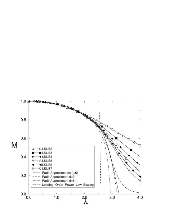
Figure 4: Results for the lattice magnetisation, $M$, of the spin-half transverse Ising model on the square lattice in the ferromagnetic regime for the CCM LSUB$m$ approximation with $m=\{2,3,4,5,6,7\}$. The extrapolation of the LSUB$m$ results at each separate value of $\lambda$ is performed in two ways. The first uses Padé approximants in order to perform the extrapolation, and the second assumes a leading-order power-law scaling of the lattice magnetisation with $m^{-1}$.

References

- (1) F. Coester, Nucl. Phys. 7, 421 (1958); F. Coester and H. Kümmel, ibid. 17, 477 (1960).
- (2) H. Kümmel, K.H. Lührmann, and J.G. Zabolitzky, Phys Rep. 36C, 1 (1978).
- (3) R.F. Bishop and K.H. Lührmann, Phys. Rev. B 17, 3757 (1978).
- (4) J.S. Arponen, Ann. Phys. (N.Y.) 151, 311 (1983).
- (5) J.S. Arponen, R.F. Bishop, and E. Pajanne, Phys. Rev. A 36, 2519 (1987); ibid. 36, 2539 (1987); J.S. Arponen, R.F. Bishop, E. Pajanne, and N.I. Robinson ibid. 37, 1065 (1988).
- (6) R.F. Bishop, Theor. Chim. Acta 80, 95 (1991).
- (7) J.S. Arponen, and R.F. Bishop, Ann. Phys. (N.Y.) 207, 171 (1991); ibid. 227, 275 (1993); ibid. 227, 2334 (1993).
- (8) R.F. Bishop, in Microscopic Quantum-Many-Body Theories and Their Applications, edited by J. Navarro and A. Polls, Lecture Notes in Physics, Vol. 510 (Springer-Verlag, Berlin, 1998), p. 1.
- (9) J.W. Clark and E. Feenberg, Phys. Rev. 113, 388 (1959).
- (10) H.W. Jackson and E. Feenberg, Rev. Mod. Phys. 34, 686 (1962).
- (11) E. Feenberg, Theory of Quantum Liquids, edited by K. Binder, (Springer, New York, 1969).
- (12) J.W. Clark, in Progress in Particle and Nuclear Physics, edited by D.H. Wilkinson, Vol. 2 (Pergamon, Oxford, 1979), p. 89.
- (13) V.R. Pandharipande and R.B. Wiringa, Rev. Mod. Phys. 51, 821 (1979).
- (14) E. Krotscheck and J.W. Clark, Nucl. Phys. A333, 77 (1980).
- (15) J.W. Clark, in The Many-Body Problem: Jastrow Correlations Versus Brueckner Theory, edited by R. Guardiola and J. Ros, Lecture Notes in Physics, Vol. 138 (Springer-Verlag, Berlin, 1981), p. 184.
- (16) S. Rosati, in International School of Physics Enrico Fermi, Course LXXIX, edited by A. Molinari (North-Holland, Amsterdam, 1981), p. 73.
- (17) A. Fabrocini and S. Fantoni, in First International Course on Condensed Matter, ACIF Series, edited by D. Prosperi, S. Rosati and S. Violini, Vol. 8 (World Scientific, Singapore, 1987), p. 87.
- (18) S. Fantoni and V.R. Pandharipande, Phys. Rev. C 37, 1687 (1988).
- (19) S. Fantoni and A. Fabrocini, in Microscopic Quantum Many-Body Theories and Their Applications, edited by J. Navarro and A. Polls, Lecture Notes in Physics, Vol. 510 (Springer-Verlag, Berlin, 1998), p. 119.
- (20) R.F. Bishop, J.B. Parkinson, and Y. Xian, Phys. Rev. B 44, 9425 (1991).
- (21) R.F. Bishop, R.G. Hale, and Y. Xian, Phys. Rev. Lett. 73, 3157 (1994).
- (22) C. Zeng and R.F. Bishop, in Coherent Approaches to Fluctuations, edited by M. Suzuki and N. Kawashima, (World Scientific, Singapore, 1996), p. 296.
- (23) D.J.J. Farnell, S.A. Krüger, and J.B. Parkinson, J. Phys.: Condens. Matter 9, 7601 (1997).
- (24) C. Zeng, D.J.J. Farnell, and R.F. Bishop, J. Stat. Phys. 90, 327 (1998).
- (25) R.F. Bishop, D.J.J. Farnell, and J.B. Parkinson Phys. Rev. B 58, 6394 (1998).
- (26) R.F. Bishop and D.J.J. Farnell, Mol. Phys. 94, No. 1, 73 (1998).
- (27) R.F. Bishop, D.J.J. Farnell, and Chen Zeng, Phys. Rev. B 59, 1000 (1999).
- (28) J. Rosenfeld, N.E. Ligterink, and R.F. Bishop, Phys. Rev. B 60, 4030 (1999).
- (29) M.L. Ristig and J.W. Kim, Phys. Rev. B 53, 6665 (1996).
- (30) M.L. Ristig, J.W. Kim, and J.W. Clark, in Theory of Spin Lattices and Lattice Gauge Models, edited by J.W. Clark and M.L. Ristig, Lecture Notes in Physics, Vol. 494 (Springer-Verlag, Berlin 1997), p. 62.
- (31) M.L. Ristig, J.W. Kim, and J.W. Clark, Phys. Rev. B 57, 56 (1998).
- (32) R.F. Bishop, D.J.J. Farnell, and M.L. Ristig, in Condensed Matter Theories, Vol. 14, (1999) – in press.
- (33) J. Carlson, Phys. Rev. B 40, 846 (1989).
- (34) T. Barnes, D. Kotchan, and E. S. Swanson, Phys. Rev. B 39, 4357 (1989).
- (35) N. Trivedi and D.M. Ceperley, Phys. Rev. B 41, 4552 (1990).
- (36) K.J. Runge, Phys. Rev. B 45, 12292 (1992); ibid. 45, 7229 (1992).
- (37) M. Boninsegni, Phys. Rev. B 52, 15304 (1995).
- (38) B. B. Beard and U.J. Wiese, Phys. Rev. Lett. 77, 5130 (1996).
- (39) A.W. Sandvik, Phys. Rev. B 56, 11678 (1997).
- (40) M.C. Buonaura and S. Sorella, Phys. Rev. B 57, 11445 (1998).
- (41) P.G. de Gennes, Solid State Comm. 1, 132 (1963).
- (42) R. Blinc, J. Phys. Chem. Solids 13, 204 (1960).
- (43) S. Katsura, Phys. Rev. 127, 1508 (1962).
- (44) M. Suzuki, Prog. Theor. Phys. 46, 1337 (1971); ibid. 56, 1454 (1976).
- (45) B.K. Chakrabarti, A. Dutta, and P. Sen, in Quantum Ising Phases and Transitions in Transverse Ising Models, Lecture Notes in Physics, Vol. m 41 (Springer-Verlag, Berlin 1996).
- (46) D.C. Mattis, in The Theory of Magnetism II: Thermodynamics and Statistical Mechanics, Springer Series in Solid-State Sciences, Vol. 55 (Springer-Verlag, Berlin, Heidelberg, New York, Tokyo 1985), p. 109.
- (47) Y. -L. Wang and B.R. Cooper, Phys. Rev. 172, 539 (1968); ibid. 185, 696 (1969).
- (48) P. Pfeuty and R.J. Elliot, J. Phys. C 4, 2370 (1971).
- (49) Zheng Weihong, J. Oitmaa, and C.J. Hamer, J. Phys. A 23, 1775 (1990); ibid. A 27, 5425 (1994).
- (50) R.B. Pearson, Phys. Rev. A 18, 2655 (1978).