From Minority Games to real markets

Abstract

We address the question of market efficiency using the Minority Game (MG) model. First we show that removing unrealistic features of the MG leads to models which reproduce a scaling behavior close to what is observed in real markets. In particular we find that i) fat tails and clustered volatility arise at the phase transition point and that ii) the crossover to random walk behavior of prices is a finite size effect. This, on one hand, suggests that markets operate close to criticality, where the market is marginally efficient. On the other it allows one to measure the distance from criticality of real market, using cross-over times. The artificial market described by the MG is then studied as an ecosystem with different species of traders. This clarifies the nature of the interaction and the particular role played by the various populations.

]

I Introduction

The Minority Game[1, 3] (MG) was initially designed as the most drastic simplification of Arthur’s famous El Farol’s Bar problem [4]: it describes a system where many heterogeneous agents interact through a price system they all contribute to determine. The MG is an highly stylized model of such a situation: it captures some key features of a generic market mechanism and the basic interaction between agents and public information – i.e. how agents react to information and how these reactions modify the information itself. In addition, it allows to study in details how macroscopic quantities depend on microscopic behaviors.

However, the basic MG is a so stylized model of a financial market that prices are not even explicitly defined. Furthermore the micro-economic behavior of agents is quite simplified: agents have heterogeneous strategies but they enter the game with the same weight. In other words there are not poorer or richer agents and their wealth does not change according to their performance. Also all agents are constrained to play, with the same frequency, no matter how much they may loose. All these unrealistic features makes it hard to accept the MG as a model of a real financial market, especially when compared to other agent-based models [5, 6, 7, 8] which have so far been more successful in reproducing the stylized facts of high frequency statistics of prices [9].

The same stylized nature of the MG however, allows one to gain a deep understanding of its extremely rich collective behavior: Statistical mechanics of disordered systems indeed allows for a full analytic solution in the limit of infinitely many agents [10]. More precisely, these techniques allows one to fully characterize the evolutionary equilibrium of the dynamical learning process in a truly complex system of interacting adaptive agents. In a top-down approach to real financial markets, where complexity is added in steps, the analytic solution of the MG provides an invaluable starting point which allows us to keep full control on the emergent features. Several extensions in this direction where discussed elsewhere [11, 12, 13].

The purpose of the present paper is to advance even more in this endeavor. First we show that, by removing further unrealistic features, and defining a price process in terms of excess demand, the main stylized facts of high frequency price fluctuations are recovered within the MG. In particular we allow agents to have different weights in the market according to their wealth, which evolves as a result of their trades. As in the MG we find a phase transition between a symmetric (information-efficient) phase and an asymmetric phase, depending on the ratio $\alpha$ between agents and information complexity. The symmetric phase, in this case, is characterized by zero excess demand and constant prices and is hence similar to an absorbing phase. Statistical features such as fat tails in the distribution of returns and long-time volatility autocorrelation, only arise close to the critical point $\alpha_{c}$.

Second, we derive a coherent picture of the collective behavior of a market. In this picture, we can regard a market as an ecology of different “species” of investors, each playing his particular role. On one side there are traders who need the market for exchanging goods and are not interested in speculation. These kind of agents – called hedgers in the economic literature [16] – will be called producers hereafter, following ref. [11]. On the other, there are bounded rational agents speculators equipped with inductive thinking and very heterogeneous strategies, acting as scavengers of information. We can offer a coherent picture of how the resulting food chain operates: Producers inject a limited amount of information, upon which a swarm of speculators feed. The two groups in the market ecology have only partial overlap in interest. This calls for two parameters to characterize efficiency because market efficiency is interpreted differently from different players. Producers would like that the information content is small, and fluctuations also. Whereas speculators would like small fluctuations, but they prefer when the information content is large.

Thus the MG provides a coherent picture of how markets function which, on one hand is rooted on an analytic approach providing deep insights on the collective statistical behavior and, on the other, is able to reproduce the main statistical regularities – the so-called stylized facts – of financial markets.

We keep our discussion as simple and informal as possible. Formal mathematical definitions and technical details can be found in the appendix.

II The MG as a coarse grained model of a market

Naively speaking, what agents do in a financial market is to gather information on the present state of the market and to process it in order to determine an investment strategy. We call this mapping from information to action a trading strategy. One can regard a market as an “evolutionary soup” of trading strategies competing against each other[2, 21]. Modeling this system is a quite complex task: First because trading strategies, in general, live in a very complex and high dimensional functional space (specially because of their inter-temporal nature). Secondly, trading strategies involve all sorts of details – such as expectations, beliefs, how agents behave under uncertainty and how they discount the future – which are heterogeneous across agents. Finally time constraints and information or computational complexity may induce agents to a sub-optimal, boundedly rational behavior [4].

This situation forces one either to models whose complexity is of the same order of reality, and that are hence useless, or to work under some simplifying assumptions. The MG is based on the following simplifications:

1. time is discrete, i.e. market interaction is repeated for a infinitely many periods.

2. information is discretized in one of $P$ events labeled by an integer $\mu$, which is drawn at random, independently in each period[22].

3. actions are discretized in a binary choice $a_{i}(t)\in\{-1,1\}$ at each period $t$ for each agent $i$

4. The space of trading strategies is then the set of binary functions $f:(1,\ldots,\mu,\ldots,P)\to(-1,+1)$.

5. Agents are heterogeneous: Each agent is endowed with a finite number $S$ of trading strategies, which are drawn at random and independently for each agent from the set of all possible strategies.

6. Agents are adaptive: they evaluate the performance of their strategies while using their best one for actual trading. The adaptive process is similar reinforcement learning dynamics [23, 24] but traders behave non-strategically, i.e. as price-takers (see ref. [10] for more details).

7. the market mechanism is a minority game: Agents who took the minority action are rewarded whereas the majority of agents loses. This captures the fact that markets are mechanisms for reallocation of resources so that no gain is possible, in principle, by pure trading. If some agent gains, some other must lose. With $A(t)=\sum_{i}a_{i}(t)$ being the sum of individual actions $a_{i}(t)$, a simple choice of payoffs of minority type is

   $$u_{i}(t)=-a_{i}(t)A(t).$$ (1)

   If $A(t)>0$, traders who took $a_{i}(t)=-1$ win, whereas those who took $a_{i}(t)=+1$, which are the majority, loose.

This is a coarse grained description of a market in the sense that it does not enter into the details of the behavior of agents nor of the market mechanism. Both are considered as black boxes containing all sorts of complications. We just retain the key features of i) heterogeneity and bounded rationality for agents, and ii) the minority nature for the market mechanism.

It needs to be said that such a coarse description also requires an abstraction of usual terms such as prices, volume and excess demand at a more generic level. For example it is natural to relate $A(t)$ – which is the unbalance between the two group of agents – to the excess demand. Indeed the latter measures in a real market the unbalance between buyers and sellers. In view of the statistical nature of the laws which govern the collective behavior, and of the robustness of these laws with respect to changes in microscopic details, such a stretch of the customary meaning of common economic terms may be justified.

It is also worth stressing that there is no a priori best trading strategy in the market depicted by the Minority Game. This justifies the equiprobability assumption by which strategies are drawn. Whether a strategy is good or bad cannot be decided a priori; rather the quality of a strategy depends on how it will perform against the other strategies present in the market.

The two features discussed above are enough to reproduce a remarkably rich behavior: The key variable is the ratio $\alpha=P/N$ between information diversity $P$ and the number $N$ of agents [19]. The collective behavior is characterized by market’s predictability $H$, and global efficiency $\sigma^{2}$ (see appendix I). The first ($H$) measures how the market outcome $A(t)$ is correlated with the information $\mu(t)$, i.e. whether a positive $A(t)$ is more or less likely than a negative one when the information is $\mu$. $H>0$ implies that knowledge of $\mu$ allows some prediction of the sign of $A(t)$; accordingly some agents have a positive gain. The second ($\sigma^{2}=-\sum_{i}\langle{u_{i}}\rangle$) is related to the total loss suffered by agents, which means that the MG is a negative sum game. When few agents are present (large $\alpha$) the market is easily predictable (i.e. $H>0$) and agents perform only slightly better than random agents (who decide their actions on the basis of coin tossing). As more and more agents are added, the market becomes more efficient both because agents payoffs increase on average (i.e. $\sigma^{2}$ decreases) and because the market becomes less predictable (i.e. $H$ decreases). A phase transition takes place [19, 17, 18] at a critical value $\alpha_{c}$, where agents average gain reaches a maximum and the market’s outcome becomes unpredictable [17] ($H=0$). Below this value of $\alpha$ the market remains unpredictable ($H=0$) and the losses of agents ($\sigma^{2}$) increase in a way which is specially dramatic if agents are very reactive [20]. All these features generalize to a number of situations such as i) including a fraction of deterministic agents – so called producers or hedgers [16] – who have but one strategy and can make the market a positive sum game[11], ii) allowing for some correlation in the pool of strategies held by each agent [11], or iii) allowing for agents with different constant weights. The phase diagram for this last case is reported in Fig. 1 (see the appendix for details on the calculation).

FIG. 1.: Phase diagrams of the MG with weighted agents for different distributions of weights $w_{i}$: power law (full line) and stretched exponential (dotted line) distribution with parameter $\gamma$. The results for a uniform distribution is also shown as a dashed line. Below the line corresponding to each distribution, the market is in the symmetric phase $H=0$.

The emergent picture is that when agents are few, the market is rich of profitable trade opportunities. These may attract other agents in the market. As the number of agents increases, these opportunities are eliminated and the market is driven towards information efficiency ($H=0$). This suggests that the real markets should operate close to the critical point $\alpha_{c}$ where profitable trade opportunities are barely detectable. The process by which the market self-organizes close to the critical point is more likely to be of evolutionary nature and hence to take place on longer time-scales

There are two unnatural features in the MG at this stage: First agents are always constrained to play, even if they lose a lot, and second the performance of an agent does not affect his wealth. In reality each trader is allowed only to lose a finite amount of money, after which it goes bankrupt and exits the game. In the following we shall see that the correction to these two shortcomings leads indeed to quite realistic results .

III The MG with dynamical capitals

How is this scenario modified if one accounts for the fact that agents have a fixed budget $c_{i}$ which itself evolves as a result of their trading? We address this issue by making $c_{i}(t)$ – the capital held by agent $i$ at time $t$ – a dynamical variable and assuming that each agent $i$ invests a fraction $\epsilon$ of it in the market. Speculators have no other gain than that resulting from trading, so that $c_{i}(t)$ evolves as a result of it. On the other hand, producers – who have other revenues and use the market for reallocation of resources – always invest a fixed quantity (see the appendix for more details). In a loose sense the model becomes evolutionary. Indeed poorly performing strategies lead to capital losses and are therefore washed out of the market. On the other hand good strategies imply capital increase, which enhances the negative effects of market impact. As a result capitals adjust in order to balance strategy’s performance and market impacts.

Similar models with dynamical capitals, based on the minority game, have been studied in refs. [14, 15]. Ref. [14] expands in much details on the micro-economics of these types of models and explores how collective behavior depends on it. The agent based models discussed in ref. [15] pay also considerable attention to realism at the micro-economic level. The price for this is that one needs to introduce many parameters which implies that one looses the contact with picture provided by the analytic solution to the MG[18]. Our approach is instead based on this picture and aims primarily at establishing what elements of this picture persist when the complexity of the model increases. Key questions, for us, are whether the phase transition is robust to such changes and whether anomalous scaling of price returns [9] are related to the critical point or not. As we shall see, we find positive answers in both cases, which open a new perspective on market’s efficiency.

FIG. 2.: Behavior of the MG with dynamic capitals as a function of $\alpha$: fluctuation of returns $\langle{r^{2}}\rangle$ ($\circ$) and average wealth of speculators ($\diamond$). The system is composed of $50$ producers and $50$ speculators. Simulations were carried out for a number of time steps large enough to reach a stationary state (which typically requires $10^{6}$ time steps). The results depend very weakly on $\epsilon$, as long as it is small, and on the distribution of wealth of producers: A power law distribution with exponent $3/2$ (open symbols) yields very similar results to those obtained with an exponential distribution (full symbols).

The results of numerical simulations, as a function of $\alpha$ are shown in figure 2. As the information complexity $P$ decreases (or as number of agents increases) i.e. as $\alpha$ decreases, the market becomes less and less predictable. Again at a critical value $\alpha_{c}$ the market becomes unpredictable. Actually the dynamics of $c_{i}(t)$ reaches a point where the return $r^{\mu}$ to the investment under information $\mu$ vanishes for all $\mu=1,\ldots,P$. Hence the phase $\alpha<\alpha_{c}$ is an absorbing phase where no dynamics actually takes place. The statistical properties of the stationary state are in principle accessible to an analytic approach along the lines of refs. [18, 10] for $\epsilon\ll 1$ as discussed in the appendix. Interestingly, $\alpha_{c}$ marks also the point where the relative wealth of speculators is maximal, as can be seen in fig. 2. The distribution of wealth across agents falls off exponentially, with a characteristic wealth which is maximal at $\alpha_{c}$.

FIG. 3.: Probability density function (pdf) of returns (rescaled to unit variance) for $\alpha=0.64=\frac{260}{401}$, $0.80=\frac{240}{301}$, $1.09=\frac{220}{201}$, $1.98=\frac{200}{101}$. Tails become fatter and fatter as the critical value $\alpha_{c}\approx 0.6$ is approached.

Having defined returns from trading, allows one to define a price $p(t)$ as the sum over time of returns (see the appendix for more details). Then one can investigate the statistical properties of the price time series and compare it to empirical findings [9]. Remarkably figure 3 shows that fat tails similar to those observed in real markets emerge close to the critical point $\alpha_{c}$. In addition figure 4 shows that volatility clustering also emerges close to the critical point: The correlation function of absolute values of returns has an algebraic decay with time close to $\alpha_{c}$ which turns into an exponential decay away from criticality.

FIG. 4.: Volatility correlation function $\langle{|r(t)||r(0)|}\rangle-\langle{|r(0)|}\rangle^{2}$ of absolute returns for $\alpha=0.64=\frac{260}{401}$, $0.80=\frac{240}{301}$, . Exponent of the autocorrelation function is about -0.64 for $\alpha=0.64$

The dynamics of $c_{i}(t)$ gives an evolutionary character to the model, because poorly performing agents are driven out of the market. Indeed, asymptotically, a finite fraction of agents end up with $c_{i}=0$. Evolutionary selection in the market can be introduced assuming that agents with $c_{i}<\bar{w}\ll 1$ are replaced by new agents, which enter with an initial capital $c_{i}=1$ and random trading strategies. A further modification of the model lies in removing the unrealistic feature of forcing agents to trade at each time step. It seems reasonable to allow agents not to trade, if their trading strategies perform poorly [15]. The phase transition separating an information efficient phase $\alpha<\alpha_{c}$, from an inefficient phase $\alpha>\alpha_{c}$ survives to all these modifications. Fig. 5 shows that the rescaled pdf of returns on different time lags $\Delta t$ collapse quite well close to $\alpha_{c}\approx 0.32$ whereas a clear crossover to Gaussian behavior occurs for $\alpha=0.64$. In other words, the crossover to a Gaussian distribution of the distribution of returns $p(t+\Delta t)-p(t)$ occurs for a characteristic time lag $\Delta t_{0}$ which increases as one approaches the critical point $\alpha_{c}$. This is reminiscent of critical phenomena in statistical physics [28] where correlation length and times diverge as the distance $\alpha-\alpha_{c}$ to the critical point vanishes. In this framework of critical phenomena, the crossover to a Gaussian pdf manifests itself as a finite size scaling phenomenon. Hence a measure of crossover times $\Delta t_{0}$ in real markets allows one to estimate the parameter $\alpha$, or its distance to criticality, in that market. This calls for a systematic study of the relation between $\Delta t_{0}$ and $|\alpha-\alpha_{c}|$ which goes beyond the scope of the present paper and shall be discussed elsewhere.

It is also tempting to speculate that this relation between $\alpha$ and time-scales tells us how the number of market-relevant events over a time window $\Delta t$ increases as the window size $\Delta t$ increases. At $\alpha_{c}$, all the original $P$ events have lost their information content, hence the market is invariant under time rescaling. At $\alpha=\alpha_{c}+\epsilon$, the unexploited information remaining in the market is amplified by time rescaling. In other words, that information becomes more and more detectable on larger and larger time-scales. This is consistent with Figs. 3, 4 and 5, which show that the market at longer and longer time-scales looks less and less critical.

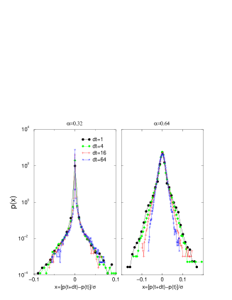
FIG. 5.: Probability density function (pdf) of returns (rescaled to unit variance) for different time lags $dt=1$, $4$, $16$ and $64$. The market is composed of $N_{s}=100$ speculators with dynamic capitals ($\epsilon=0.1$) and $N_{p}=10$ producers ($v_{i}=1$). Speculators can decide not to play and those who loose all their capital are replaced by new agent with random strategies and $c_{i}=1$. $\alpha=0.32$ (left) and $0.64$ (right).

The crossover times to Gaussian behavior can be measured in real markets. Its relation to the distance $|\alpha-\alpha_{c}|$ from the critical point may serve as a basis to classify real markets according to their distance from criticality.

IV Market’s ecology

The artificial financial market described by the Minority Game can be regarded as an ecosystem where different types of species of traders interact. The three main species are producers – who trade in a deterministic way – speculators – who are adaptive – and noise traders – who behave randomly (see the appendix). The interaction between these three species, which has been first studied in ref. [11], will be the subject of the present section.

We shall discuss the Minority Game with fixed capitals, for which we can rely on analytic results [18]. This allows us to quantify the effect of the change in concentration of one species on itself, on the other species and on the global behavior.

As a measure of the efficiency of the market, one can take the signal to noise ratio, which in the present context is just $H/(\sigma^{2}-H)$. This accounts for the fact that even if some profitable trading opportunities exist (i.e. $H>0$), they can only be detected if their intensity exceeds that of stochastic fluctuations (volatility $\sigma^{2}-H$). The signal to noise trader gives a measure of efficiency which is particularly relevant for speculators. A second measure of efficiency is volatility: Market participants take into account expected payoffs and risk, in a proportion related to their risk aversion (and their time horizon). While speculators or noise traders may be close to risk neutral, producers are risk averse; for the latter, the fluctuations are a more relevant measure of efficiency.

The impact of noise traders on the market ecology, as discussed elsewhere[11], is easy to characterize. They do not contribute to $H$, but they contribute to the losses $\sigma^{2}$. Noise traders do not affect the payoffs of other species. They only contribute to volatility (see the appendix). We shall than concentrate on the interaction between speculators and producers. Fig. 6 illustrates the effects of adding an agent to a market with a fixed number of producers, as the number of speculators varies (both numbers are computed in units of $P$, see appendix).

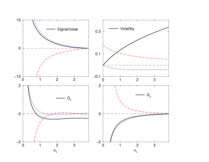
FIG. 6.: Signal to noise ratio (upper left), volatility (upper right) and payoffs of agents (lower panels; left for speculators and right for producers) for a market with $n_{p}=1$ as a function of the (reduced) number $n_{s}$ of speculators. Each graph also shows the variation of the corresponding quantities if the number of producers (dotted lines) or speculators (dashed lines) increase. The figures refer to the asymmetric phase $H>0$ ($n_{s}<n_{s}^{*}$).

The signal to noise ratio decreases if new speculators enter the market and increases as the number of producers increases. The volatility instead increases with the number of speculators and decreases with the number of producers: As the number of speculators increases, the market becomes less predictable and speculators themselves are less and less efficient in exploiting the information present in the market. This results in the increase of volatility. On the other hand, increasing the number of producers, makes speculators behave more efficiently. The payoff of producers, which is always negative, increases with the number of speculators and it decreases with the number of producers themselves. This suggests that the relationship between these two species may be better described as symbiosis than as competition. Indeed generally also the payoff of speculators increase if the number of producers increases. But as Fig. 6 shows, the situation for speculators is more complex than that: If $n_{p}$ is large enough (i.e. above the dotted line in fig. 7), the gain of speculators decreases if a other producers enter the game. Furthermore, close to the boundary $n_{s}^{*}(n_{p})$ of the symmetric phase, the gain of speculators increases if a new speculator is added. This suggests that the relationship among speculators cannot be described as competition in this region (below the dashed line in fig. 7). The phase diagram in the plane $(n_{s},n_{p})$, shown in fig. 7, summarizes this behavior.

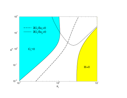
FIG. 7.: Phase diagram of the MG in the $(n_{s},n_{p})$ plane. The symmetric phase, where $H=0$, is the shaded area in the lower right corner. The payoff $G_{s}$ to speculators is positive in the upper left shaded region. Above (below) the dotted line, an increase in the number $n_{p}$ of producers causes a decrease (increase) in the payoff $G_{s}$ of speculators: i.e. $\partial G_{s}/\partial n_{p}<0$ (resp. $\partial G_{s}/\partial n_{p}>0$). The dashed line separates a region (left) where speculators are in competition (i.e. $\partial G_{s}/\partial n_{s}<0$), from a region (right) where $G_{s}$ increases with $n_{s}$.

These surprising result highlights the complexity of the interacting market system described by the minority game. The advantage of the Minority Game with respect to other agent based models, is that this complexity can be investigated analytically in detail, for simple cases.

V Conclusions

The MG is not just a toy model, but a rather good starting point for modeling markets. By removing one by one its unrealistic features, one obtains little by little stylized facts like fat tails and algebraic decay of the volatility auto-correlation function; in addition, the correspondence between stylized facts and additional features put into the MG is very instructive.

But the MG is not only able to reproduce stylized facts. It is an extremely powerful tool to explore the interplay between different types of agents, and efficiency – which can be well defined in this model. The measure of efficiency should depend on which type of agents is considered : for instance, speculators are likely to be interested in the signal to noise ratio, whereas producers are more concerned with fluctuations.

Information, the price mechanism and agents behavior in real markets may be very different from those assumed in the MG. However, if the collective behavior of the market is due to statistical laws, we expect it to be largely independent of microscopic details. From this point of view, we expect the MG can say something about real markets. For example, the phase transition from symmetric (unpredictable) to asymmetric (predictable) markets is a very robust feature of MG’s. On one hand we expect a similar transition also in real markets, on the other we showed how the distance from the critical point can be estimated.

Further efforts to calibrate the MG to reproduce the statistical features of a given market are certainly necessary to pursue this line of research.

A Definition of the MG

Let ${\cal N}$ be the set of agents engaged in the minority game and $N=|{\cal N}|$ be their number. At each time $t$ each agent $i\in{\cal N}$ takes an action $a_{i}(t)$, which is a real number quantifying his individual demand. The market interaction is defined in terms of the “excess demand” at time $t$, which is:

$$A(t)=\sum_{i\in{\cal N}}a_{i}(t)$$ (A1)

The “volume” of trades is defined as

$$V(t)=\sum_{i\in{\cal N}}|a_{i}(t)|.$$ (A2)

Let the return, at time $t$, be $r(t)=-A(t)/V(t)$ so that the payoffs to each agent $i\in{\cal N}$ is

$$g_{i}(t)=a_{i}(t)r(t)=-\frac{a_{i}(t)A(t)}{V(t)}.$$ (A3)

This structure of interaction has the minority nature discussed in the text: If $A(t)>0$ it is convenient to choose $a_{i}(t)<0$ and vice-versa.

As in refs. [6, 21, 25, 15, 14], we define a price process by:

$$\log p(t+1)=\log p(t)+r(t)=\log p(t)-\frac{A(t)}{V(t)}.$$ (A4)

These equations are also the simplest ones dictated by dimensional analysis: $g_{i}$ has the same units as excess demand $A$ and return $r$ and $\log p$ are dimensionless (note that in ref. [11] $g_{i}$ was not normalized to the number of agents).

Agents observe a public information, which can take one of $P$ forms, labeled by an integer. $\mu(t)$ is the information at time $t$, which we assume here to be randomly drawn at each time. We distinguish three types of agents according to their behavior with respect to information:

$$a_{i}(t)=\left\{\begin{array}[]{cc}{\rm rand}&i\in{\cal N}_{n}\\ v_{i}\sigma^{\mu(t)}_{i}&i\in{\cal N}_{p}\\ w_{i}\sigma^{\mu(t)}_{i,s_{i}(t)}&i\in{\cal N}_{s}\end{array}\right.$$ (A5)

The first type of agents (${\cal N}_{n}$) shall be called noise traders. They totally disregard information and take actions at random (i.e. with no correlation to $\mu(t)$). For example $a_{i}(t)=+1$ or $-1$ with equal probability. The second type, called producers (${\cal N}_{p}$), behaves in a deterministic way, given $\mu(t)$. $v_{i}$ is the amount they invest in the market and $\sigma_{i}^{\mu}$ is a random function of $\mu$ into $\{\pm 1\}$, drawn independently for each $i\in{\cal N}_{p}$. These functions are called strategies for short, but producers do not optimize their behavior: they only have one strategy. Speculators, which are the third type of traders (${\cal N}_{s}$ in Eq. (A5), instead can optimize their behavior dynamically: They have $S$ strategies, $\sigma_{i,s}^{\mu}$ labeled by the index $s=1,\ldots,S$, and can choose the one which performs better, by adjusting $s$. Strategies are again drawn randomly and independently for each $i$ and $s$. The amount $w_{i}$ invested by speculator $i$ will be discussed below. Hence ${\cal N}={\cal N}_{n}\cup{\cal N}_{p}\cup{\cal N}_{s}$ and $N=N_{n}+N_{p}+N_{s}$ where $N_{x}={\cal N}_{x}$ is the size of population of type $x=n,p$ or $s$. The MG has been introduced with $N_{n}=N_{p}=0$ and $w_{i}=1$, $\forall i\in{\cal N}_{s}$. The case $N_{n}>0$, $N_{p}>0$ has been first discussed in ref. [11], always with $w_{i}=v_{i}=1$. For these cases an analytic solution in the limit $N\to\infty$ has been found with $P/N_{s}=\alpha$, $N_{p}/N_{s}=\rho$ and $N_{n}/N_{s}=\eta$ fixed. Rather than using these parameters, we prefer to discuss our results in the rescaled population variables:

$$n_{n}=\frac{N_{n}}{P}=\frac{\eta}{\alpha},~{}~{}~{}n_{p}=\frac{N_{p}}{P}=\frac{\rho}{\alpha},~{}~{}~{}n_{s}=\frac{N_{s}}{P}=\frac{1}{\alpha}.$$ (A6)

The key quantities of interest are

$$\sigma^{2}=\overline{\langle{A^{2}}\rangle}=\frac{1}{P}\sum_{\mu=1}^{P}\langle{A^{2}|\mu}\rangle,$$ (A7)

which is proportional to the total losses of agents $\sum_{i\in{\cal N}}\langle{g_{i}}\rangle=-\sigma^{2}/V$, and

$$H=\overline{\langle{A}\rangle^{2}}=\frac{1}{P}\sum_{\mu=1}^{P}\langle{A|\mu}\rangle^{2}$$ (A8)

which measures the predictability of the market’s outcome $A(t)$. Here and below the average over $\mu$ is denoted by an overbar and the time average, conditional to $\mu(t)=\mu$ is denoted by $\langle{\cdot|\mu}\rangle$.

1 Analytic solution with $w_{i}=v_{i}=1$

The MG with speculators, producers and noise traders and fixed capitals, has been studied in ref. [11]. We refer the interested reader to that work and report here only the final expressions of the analytic solution [11] in terms of the parameters $n_{x}$:

$$H=P[1-n_{s}\hbox{erf}\,(z)]^{2}\left[\frac{1+Q}{2}n_{s}+n_{p}\right]$$ (A9)

where $n_{x}=N_{x}/P$ for $x=s,p,n$ are reduced concentrations. $Q$ is a function of $z$

$$Q=1-\frac{e^{-z^{2}}}{\sqrt{\pi}z}-\left(1-\frac{1}{2z^{2}}\right)\hbox{erf}\,(z)$$ (A10)

and $z=z(n_{s},n_{p})$ is the solution of the equation

$$2[(1+Q)n_{s}+2n_{p}]z^{2}=1.$$ (A11)

Note that $H$ only depends on $n_{s}$ and $n_{p}$. Noise traders have no effect on it. Ref. [11] finds

$$\sigma^{2}=H+P\left(\frac{1-Q}{2}n_{s}+n_{n}\right).$$ (A12)

The payoff of producers is

$$G_{p}=\sum_{j\in{\cal N}_{p}}\langle{g_{j}}\rangle=-\frac{n_{p}}{n_{s}+n_{p}+n_{n}}\left[\frac{1}{n_{s}}-\hbox{erf}\,(z)\right]$$ (A13)

and that of noise traders is simply $G_{n}=-n_{n}/(n_{s}+n_{p}+n_{n})$. The payoff of speculators is then $G_{s}=-\sigma^{2}/N-G_{p}-G_{n}$ with $N=N_{s}+N_{p}+N_{n}$. These expressions where used to produce the results in the text.

2 MG with heterogeneous weights of agents

The analytic solution generalizes easily to the case where the weights $w_{i}$ of the agents are randomly drawn from a given pdf $P(w)$ at the beginning of the game and kept fixed afterwards. For simplicity we deal with the case $n_{p}=n_{n}=0$ and $n_{s}=1\alpha>0$, though other cases are easily dealt with. Without loss of generality, we can fix the “scale” of $A(t)$ by imposing that the average wealth is $\langle{w_{i}}\rangle=1$ (a different value of $\langle{w_{i}}\rangle$ is restored by dimensional analysis). If $\langle{w_{i}^{2}}\rangle<\infty$, following the same calculation as in ref.[18, 10, 11], we find that

$$H=P\langle{w^{2}}\rangle_{w}(1+Q)\left[1-n_{s}\langle{\hbox{erf}\,(wz)}\rangle_{w}\right]^{2}$$ (A14)

where $\langle{\cdots}\rangle_{w}$ stands for averages over the distribution $P(w)$,

$$Q=1-\frac{\langle{we^{-w^{2}z^{2}}}\rangle_{w}}{\sqrt{\pi}\langle{w^{2}}\rangle_{w}z}-\left\langle\left(w^{2}-\frac{1}{2z^{2}}\right)\frac{\hbox{erf}\,(wz)}{\langle{w^{2}}\rangle_{w}}\right\rangle_{w}$$ (A15)

and $z$ is the solution of the equation

$$2z^{2}\langle{w^{2}}\rangle_{w}(Q+1)=1.$$ (A16)

The order parameter $Q$ is defined, in this case, as

$$Q=\frac{1}{N\langle{w^{2}}\rangle_{w}}\sum_{i=1}^{N}w_{i}^{2}m_{i}^{2}$$ (A17)

where $m_{i}$ is the “local magnetization” of agent $i$, i.e. the excess probability with which $i$ plays the strategy $s_{i}=+1$. Also $\sigma^{2}=H+P\langle{w^{2}}\rangle_{w}(1-Q)/2$. The phase transition occurs for a critical $n_{s}^{\star}$ such that $n_{s}^{\star}\langle{\hbox{erf}\,(wz)}\rangle_{w}=1$.

These equations hold as long as $\langle{w^{2}}\rangle_{w}$ is finite. When the second moment of $w_{i}$ diverges, i.e. when $P(w)\sim w^{-\gamma-1}$ for $w\gg 1$ with $\gamma<2$, one expects large fluctuations and no self-averaging. Indeed sums of the form $\sum_{i}w_{i}^{2}(\cdots)$, which define order parameters, are dominated by the richest agent and scale with $N$ faster than linearly ($\sum_{i}w_{i}^{2}\sim N^{2/\gamma}$). These sums do not satisfy laws of large numbers and the rescaled variable $N^{-2/\gamma}\sum_{i}w_{i}^{2}(\ldots)$ does not converge to a constant, as in the law of large numbers, but rather fluctuates for all $N$. Standard statistical mechanics approaches breaks down in these cases.

B appendix: MG with dynamical capitals

In real markets, the weight of each agent is not a fixed quantity, for instance because her capital evolves in time. Indeed, poorly performing speculators will eventually be ruined and will not participate to the market. We generalize the MG in order to account for this very important fact. Each speculator $i\in{\cal N}_{s}$ has a capital $c_{i}(t)$ and invests a fraction $\epsilon$ of it in the market: Hence $w_{i}(t)=\epsilon c_{i}(t)$. The capital of a speculator evolves in time according to his performance:

$$c_{i}(t+1)=c_{i}(t)+g_{i}(t)=c_{i}(t)[1+\epsilon\sigma_{i,s_{i}(t)}^{\mu(t)}r(t)]$$ (B1)

If agent $i$ loses ($g_{i}(t)<0$) his capital decreases and vice-versa.

Without producers, the gain of the speculators is always negative and hence the total capital of speculators decreases and tends to zero. When producers are present, the total capital of speculators adjusts so that speculators have $\langle{g_{i}}\rangle=0$ and a stationary state is possible. This is in principle accessible to an analytic calculation [18] for $\epsilon\ll 1$. In this case indeed one can rely on an adiabatic approximation where strategies adjust instantaneously to any small change in capitals $c_{i}(t)$. This implies that one may consider $c_{i}(t)$ as “quenched disorder” (as in the previous calculation) and impose, self-consistently that $\log c_{i}(t)$ is a stationary process (i.e. $\langle{\log[c_{i}(t+1)/c_{i}(t)]}\rangle=0$). Though feasible, this approach involves quite complex calculations.

REFERENCES

- [1] Challet D. and Zhang Y.-C., Physica A 246, 407 (1997) (adap-org/9708006).
- [2] Y.-C. Zhang, Europhys. News 29, 51 (1998)
- [3] See the Minority Game’s web page on http://www.unifr.ch/econophysics
- [4] Arthur W. B., Am. Ec. R., 84,406-411 (1994), Krugman ed.
- [5] T. Lux and M. Marchesi, Nature 397, 498 - 500 (1999)
- [6] G. Caldarelli , M. Marsili and Y.-C. Zhang , Europhys. Lett, 40 (5), pp. 479-484 (1997) , cond-mat/9709118
- [7] S. Solomon, Computational Finance 97, Eds. A-P. N. Refenes, A.N. Burgess, J.E. Moody, (Kluwer Academic Publishers 1998), cond-mat/9803367
- [8] R. Cont and J.-P. Bouchaud, preprint cond-mat/9712318
- [9] R. Mantegna and E. Stanley, Introduction to Econophysics, Cambridge University Press, 1999
- [10] M. Marsili, D. Challet and R. Zecchina, Physica A 280, 522 (2000), preprint cond-mat/9908480
- [11] Challet D., M. Marsili and Y.-C. Zhang, Physica A 276, 284 (2000) preprint cond-mat/9909265
- [12] A. De Martino and M. Marsili, preprint cond-mat/0007397
- [13] A. Cavagna, J.P. Garrahan, I. Giardina, D. Sherrington, Phys. Rev. Lett. 83, 4429 (1999) preprint cond-mat/9903415 (1999).
- [14] J. D. Farmer and S. Joshi, Santa Fe Institute working paper 99-10-071.
- [15] P. Jefferies, M.L. Hart, P.M. Hui, N.F. Johnson, preprint cond-mat/9910072 and cond-mat/000838.
- [16] H. Working, Am. Econ. Rev. 43, 314 (1953).
- [17] D. Challet and M. Marsili, Phys. Rev. E 60, 6271 (1999), preprint cond-mat/9904071
- [18] D. Challet, M. Marsili and R. Zecchina, Phys. Rev. Lett. 84, 1824 (2000), preprint cond-mat/9904392
- [19] Savit R., Manuca R., and Riolo R., Phys. Rev. Lett. 82(10), 2203 (1999), preprint adap-org/9712006.
- [20] M. Marsili and D. Challet, submitted to Adv Compl. Sys., preprint cond-mat/0004376
- [21] J. D. Farmer, Santa Fe Institute working paper 98-12-117
- [22] A. Cavagna, Phys. Rev. E 59, R3783 (1999).
- [23] A. Rustichini, Games and Econ. Behav. 29, 244 (1999).
- [24] The learning process is similar to the one described in C. Camerer and T.-H. Ho, Econometrica 67, 827 (1999) with .
- [25] J.-P. Bouchaud, R. Cont, preprint cond-mat/9801279
- [26] J. D. Farmer, Comp. Fin., Nov-Dec (1999), pp. 26-39
- [27] D. Challet and M. Marsili, Phys. Rev. E 62, 1862 (2000).
- [28] H. E. Stanley, Introduction to phase transitions and critical phenomena (Oxford, Clarendon Press, 1971).
- [29] R. Dickman et al., Brazilian J. of Phys. 30, 27 (2000) (also eprint cond-mat/9910454).