Initial-state dependence in time-dependent density functional theory

Abstract

Time-dependent density functionals in principle depend on the initial state of a system, but this is ignored in functional approximations presently in use. For one electron, it is shown that there is no initial-state dependence: for any density, only one initial state produces a well-behaved potential. For two non-interacting electrons with the same spin in one-dimension, an initial potential that makes an alternative initial wavefunction evolve with the same density and current as a ground state is calculated. This potential is well-behaved, and can be made arbitrarily different from the original potential.

I Introduction and conclusions

Ground-state density functional theory[1, 2] has had an enormous impact on solid-state physics since its invention, and on quantum chemistry in recent years [3]. Time-dependent density functional theory (TDDFT) allows the external potential acting on the electrons to be time-dependent, and so opens the door to a wealth of interesting and important phenomena that are not easily accessible, if at all, within the static theory. Important examples include atomic and molecular collisions[4], atoms and molecules in intense laser fields[5], electronic transition energies and oscillator strengths[6, 7], frequency-dependent polarizabilities and hyperpolarizabilities, etc.[8], and there has been an explosion of time-dependent Kohn-Sham calculations in all these fields. In almost all these calculations, the ubiquitous adiabatic local density approximation (ALDA)[9, 10] is used to approximate the unknown time-dependent exchange-correlation potential, i.e., $v_{\scriptscriptstyle\rm XC}^{\rm ALDA}[n]({\bf r}t)=v_{\scriptscriptstyle\rm XC}^{\rm unif}(n({\bf r}t))$, where $v_{\scriptscriptstyle\rm XC}^{\rm unif}(n)$ is the ground-state exchange-correlation potential of a uniform electron gas of density $n$. While this seems adequate for many purposes[11], little is known about its accuracy under the myriad of circumstances in which it has been applied.

Runge and Gross[12] formally established time-dependent density functional theory (TDDFT), showing that for a given initial state, the evolving density uniquely identifies the (time-dependent) potential. This established the correspondence of a unique non-interacting system to each interacting system and so a set of one-particle Kohn-Sham equations, much like in the static theory. This one-to-one mapping between densities and potentials is the time-dependent analog of the Hohenberg-Kohn theorem, but with a major difference: in the time-dependent case, the mapping is unique only for a specified initial state. The functionals in TDDFT depend not only on the time-dependent density but also on the initial state. This dependence is largely unexplored and indeed often neglected, for example in the ALDA for the exchange-correlation potential mentioned above.

What do we mean by an initial-state dependence? In the ground-state theory, there is a simple one-to-one relation between ground-state densities and Kohn-Sham potentials $v_{\scriptscriptstyle\rm S}$, assuming they exist. For example, for one electron in one dimension, we can easily invert the Schrödinger equation, to yield

$$v_{\scriptscriptstyle\rm S}(x)=\frac{d^{2}{\sqrt{n(x)}}/dx^{2}}{2{\sqrt{n(x)}}}+\epsilon$$ (1)

where $n(x)$ is the ground-state density. We use atomic units throughout ($\hbar=m=e^{2}=1$). For $N$ electrons in three dimensions, one can easily imagine continuously altering $v_{\scriptscriptstyle\rm S}({\bf r})$, the Kohn-Sham potential, solving the Schrödinger equation, finding the orbitals and calculating their density, until the correct $v_{\scriptscriptstyle\rm S}({\bf r})$ is found to reproduce the desired density. By the Hohenberg-Kohn theorem, this potential is unique, and several clever schemes for implementing this idea appear in the literature [13, 15, 16, 17, 18, 19, 20, 21]. This procedure could in principle be implemented for interacting electrons, if a sufficiently versatile and accurate interacting Schrödinger equation-solver were available.

Now consider the one-dimensional one-electron density

$$n(x)=2x^{2}\ \exp(-x^{2})/{\sqrt{\pi}},$$ (2)

(actually the density of the first excited state of a harmonic oscillator) . If we consider this as a ground-state density, we are in for an unpleasant surprise. Feeding it into Eq. (1), we find that the potential which generates this density is parabolic almost everywhere ($x^{2}/2$), but has a nasty unphysical spike at $x=0$, of the form $\delta(x)/|x|$. We usually exclude such potentials from consideration[22], and regard this density as not being $v$-representable.

But now imagine that density as being the density of a first excited state. In that case, the relation between density and potential is different, because the orbital changes sign at the node. The mapping becomes

$$v_{\scriptscriptstyle\rm S}(x)=\frac{d^{2}\left({\rm sgn}(x-x_{0}){\sqrt{n(x)}}\right)/dx^{2}}{2\left({\rm sgn}(x-x_{0}){\sqrt{n(x)}}\right)}+\epsilon$$ (3)

where ${\rm sgn}(x)=1$ for $x>0$ and -1 for $x<0$, and $n(x_{0})=0$. If we use this mapping, we find a perfectly smooth parabolic well ($x^{2}/2)$. This is a simple example of how the mapping between densities and potentials depends on the initial state.

More generally, for any given time-dependent density $n({\bf r}t)$, we ask how the potential $v({\bf r}t)$ whose wavefunction yields that density depends on the choice of initial wavefunction $\Psi_{0}$, i.e., in general $v[\Psi_{0},n]({\bf r}t)$. Our aim in this paper is to explicitly calculate two different potentials giving rise to the same time-dependent density by having two different initial states. Note that even finding such a case is non-trivial. The choice of wavefunctions is greatly restricted by the time-dependent density. As van Leeuwen has pointed out [23], the continuity equation $\dot{n}=-\nabla\cdot{\bf j}$ implies that only wavefunctions that have the correct initial current are candidates for generating a given time-dependent density. Van Leeuwen also shows how to explicitly construct the potential generating a given density from an allowed initial wavefunction using equations of motion.

Why is this important? The exchange-correlation potential, $v_{\scriptscriptstyle\rm XC}({\bf r}t)$, of TDDFT is the difference between a Kohn-Sham potential and the sum of the external and Hartree potentials. Since both the interacting and non-interacting mappings can depend on the choice of initial state, this potential is a functional of both initial states and the density, i.e., $v_{\scriptscriptstyle\rm XC}[n,\Psi_{0},\Phi_{0}]({\bf r}t)$. But in common practice, only the dependence on the density is approximated. We show below that this misses significant dependences on the initial state, which can in turn be related to memory effects, i.e., dependences on the density at prior times.

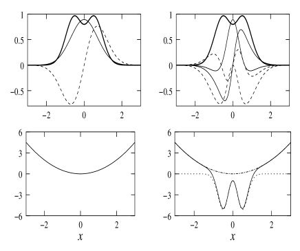
FIG. 1.: The top left-hand plot shows the ground-state orbitals $\phi_{1}$ (solid) and $\phi_{2}$ (dashed) and their density $n$ (thick solid line) for the harmonic potential in the lower left-hand plot. The top right-hand plot contains the real and imaginary parts of alternative orbitals $\tilde{\phi}_{1}$(solid) and $\tilde{\phi}_{2}$(dashed), and their density, $n$(thick solid), while below is the unique initial potential $\tilde{v}$ (solid line) that keeps the density constant.

In the special case of one electron, we prove in section II A that only one initial state has a physically well-behaved potential. Any attempt to find another initial state which evolves in a different potential with the same evolving density, results in a “pathological” potential. The potential either has the strong features at nodes mentioned above, or rapidly plunges to minus infinity at large distances where the density decays. (How such a potential can support a localized density is discussed in section III.) Such non-physical states and potentials are excluded from consideration (as indeed they are in the Runge-Gross theorem). Thus there is no initial-state dependence for one electron.

We might then reasonably ask, can we ever find a well-behaved potential for more than one allowed initial wavefunction? The answer is yes, which we demonstrate with a specific example. Consider two non-interacting electrons of the same spin in a harmonic well. In the ground state of this two electron system, the first electron occupies the oscillator ground state, and the second occupies the first excited state, as shown in Fig. 1. If we keep the potential constant, the density will not change. By multiplying each orbital by a spatially varying phase, and choosing these phases to make the current vanish, we find an allowed alternative initial state (see section III for details). Van Leeuwen’s prescription then yields the unique potential which makes this wavefunction evolve with the same density. The difference is perfectly well-behaved, and can be made arbitrarily large by adjusting a constant in the phases of the alternative orbitals. To our knowledge, this is the first explicit construction of two different potentials that yield the same time-dependent density. Other examples are given in section III.

Now imagine the density of Fig. 1 were the ground-state density of some interacting two-electron system, in some external potential $v_{\rm ext}(x)$. Then both potentials shown in lower panels of Fig. 1 are possible Kohn-Sham potentials, $v_{\scriptscriptstyle\rm S}(x)$, for this system. Since the Hartree potential is uniquely determined by the density, we have two very different exchange-correlation potentials, differing by the amount shown. In fact, different choices of initial wavefunction allow us to make the two dips arbitrarily deep or small. Any purely density functional approximation misses this effect entirely, and will produce the same exchange-correlation potential for all cases.

So, even in the simplest case of non-degenerate interacting and Kohn-Sham ground states, one can choose an alternative Kohn-Sham initial state, whose potential will look very different from that which evolves from the initial ground state. In practice, the majority of applications of TDDFT presently involve response properties of the ground-state of a system, and one naturally choses to start the Kohn-Sham system in its ground state. This choice is also dictated by the common use of adiabatic approximations for exchange-correlation potentials, which are approximate ground-state potentials evaluated on the instantaneous density. Such models will clearly be inaccurate even at $t=0$ if we start our Kohn-Sham calculation in any state other than its ground state.

The initial-state dependence of functionals is deeply connected to the issue of memory effects which are ignored in most TDDFT functional approximations used today. Yet these can often play a large role in exchange-correlation energies in fully time-dependent (i.e. non-perturbative) calculations[24] as well as giving rise to frequency-dependence of the exchange-correlation kernel in linear response theory ($f_{\scriptscriptstyle\rm XC}(\omega)$) [25]. Functionals in general depend not only on the density at the present time, but also on its history. They may have a very non-local (in time) dependence on the density. But still more about the past is required: the functional is also haunted by the initial wavefunction. The initial state dependence is inextricably linked to the history of the density and in fact can be absorbed into density-dependence along a pseudo pre-history [26]. The results of this current paper shed some light on the importance of memory effects arising from the initial wavefunction.

To summarize, we have shown that there is no initial-state dependence for one electron, and that there can be arbitrarily large initial-state dependence for two electrons.

II Theory

Consider a density $n({\bf r}t)$ evolving in time under a (time-dependent) potential $v({\bf r}t)$. Can we obtain the same evolving density $n({\bf r}t)$ by propagating some different initial state in a different potential $\tilde{v}({\bf r}t)$? This was answered in the affirmative in Ref. [23] under the condition that the two initial states have the same initial density and initial first time-derivative of the density. Here we shall show that additional restrictions are required on the initial state for this statement to hold. In the one-electron case, the additional restrictions are so strong that there is no other initial state that evolves with the same density as another does in a different potential.

A One electron

Any two one-electron wavefunctions $\phi({\bf r}t)$ and $\tilde{\phi}({\bf r}t)$ with the same density $n({\bf r}t)=|\phi({\bf r}t)|^{2}=|\tilde{\phi}({\bf r}t)|^{2}$, are related by a spatial and time dependent phase factor:

$$\tilde{\phi}({\bf r}t)=\phi({\bf r}t)\ \exp\left(i\alpha({\bf r}t)\right)$$ (4)

where the phase $\alpha({\bf r}t)$ is real. The evolution of each wavefunction is determined by the time-dependent Schrödinger equation with its potential (dot implies a time derivative):

$$\left(-\nabla^{2}/2+v({\bf r}t)\right)\phi({\bf r}t)=i\dot{\phi}({\bf r}t).$$ (5)

Both will satisfy the continuity equation:

$$\dot{n}({\bf r}t)=-\nabla\cdot{\bf j}({\bf r}t)$$ (6)

where the current density of a wavefunction $\phi$ is

$${\bf j}({\bf r}t)=i\left(\phi({\bf r}t)\nabla\phi^{*}({\bf r}t)-\phi^{*}({\bf r}t)\nabla\phi({\bf r}t)\right)/2.$$ (7)

Substituting $\tilde{\phi}({\bf r}t)$ from Eq. (4) into Eq. (7), we obtain

$$\Delta{\bf j}({\bf r}t)=n({\bf r}t)\nabla\alpha({\bf r}t).$$ (8)

(We use the notation $\Delta a$ to denote $\tilde{a}-a$.) Because the densities are the same for all times, $\Delta\dot{n}({\bf r}t)=0$, so by Eq. (6)

$$\nabla\cdot[n({\bf r}t)\nabla\alpha({\bf r}t)]=0$$ (9)

Integrating Eq. (9) with $\alpha({\bf r}t)$ and performing the integral by parts, we find

$$\int d^{3}r\ n({\bf r}t)|\nabla\alpha({\bf r}t)|^{2}=0.$$ (10)

We have taken the surface term $\int d^{2}{\bf S}\cdot(\alpha n\nabla\alpha)$ evaluated on a closed surface at infinity, to be zero: this arises from the physical requirement that at infinity, where the electron density decays, any physical potential remains finite. (In fact this condition is required in the proof of the Runge-Gross theorem [12]). If the surface term did not vanish, then $\alpha\nabla\alpha$ must grow at least as fast as $(r^{2}n(\bf r))^{-1}$ as $r$ approaches infinity. This would lead to a potential that slides down to $-\infty$ which can be seen by inversion of the time-dependent Schrödinger equation in the limit of large distances. The state would oscillate infinitely wildly at large distances in the tails of the density but the decay of the density is not enough to compensate for the energy that the wild oscillations impart: this state would have infinite kinetic energy, momentum and potential energy. (We shall see this explicitly in section III A). So for physical situations, the surface term vanishes.

Because the integrand above cannot be negative, yet it integrates to zero, the integrand itself must be zero everywhere. Thus $\nabla\alpha({\bf r}t)=0$ everywhere except perhaps at nodes of the wavefunction where $n({\bf r}_{0}t)=0$. In fact, even at the nodes, $\nabla\alpha({\bf r}_{0}t)=0$ to avoid highly singular potentials: if $\nabla\alpha$ was finite at the nodes and zero everywhere else, then as a distribution, it is equivalent to being zero everywhere, for example its integral $\alpha$ is constant. There remains the possibility that $\nabla\alpha$ is a sum of delta functions centered at the nodes, however this leads to potentials which are highly singular at the nodes, as in the introduction. Such unphysical potentials are excluded from consideration, so that $\nabla\alpha({\bf r}t)=0$, or $\alpha({\bf r}t)=c(t)$. The wavefunctions $\phi({\bf r}t)$ and $\tilde{\phi}({\bf r}t)$ can therefore differ only by an irrelevant time-dependent phase. In particular, this means that only one initial state and one potential can give rise to a particular density, i.e, the evolving density is enough to completely determine the potential and initial state.

The one-electron case is a simple counter-example to the conclusions in Ref. [23], which rely on the existence of a solution to

$$\nabla\cdot[n\nabla\Delta v]=\eta({\bf r}t),$$ (11)

where $\eta({\bf r}t)$ involves expectation values of derivatives of the momentum-stress tensor and derivatives of the interaction (see section II B). This is to be solved for the potential subject to the requirements that the two initial states have the same $n({\bf r}0)$ and $\dot{n}({\bf r}0)$, and that $\nabla\Delta v\to 0$ as $r\to\infty$. The two initial wavefunctions in the one-electron case have the same initial $n({\bf r}0)$ (Eq. 4) and $\dot{n}({\bf r}0)$ (Eq. 9) but no two physical potentials exist under which they would evolve with the same density, because there is no solution to Eq. (11) subject to the boundary condition that $\nabla\Delta v=0$. (For an explicit demonstration of this in one-dimension, see section III A.) We shall come back to this point at the end of section II B.

B The many-electron case

In this section we follow van Leeuwen’s prescription to find the potential needed to make a given initial state evolve with the same density as that of another. However we simplify the equations there somewhat to make the search for the solution of the potential easier. Given an initial state $\Psi_{0}$ which evolves with density $n({\bf r}t)$ in a potential $v({\bf r}t)$, we solve for the potential $\tilde{v}({\bf r}t)$ in which a state $\tilde{\Psi}$ evolves with the same density $n({\bf r}t)$. If we require $\tilde{\Psi}$ to have the same initial density and initial first time-derivative of the density, then a solution for $\tilde{v}$ may be obtained from equating the equations for the second derivatives of the density for each wavefunction, subject to an appropriate boundary condition like $\Delta v\to 0$ at large distances. We are not guaranteed that such a solution exists: the wavefunction must have the additional restriction that the initial potential computed in this way is bounded at infinity.

The equation of motion for $\dot{n}$ yields (Eq. (15) of Ref. [23]):

$$\ddot{n}({\bf r}t)=\nabla\cdot\left[n({\bf r}t)\nabla v({\bf r}t)+{\bf t}({\bf r}t)+{\bf f_{\rm ee}}({\bf r}t)\right]$$ (12)

where

$${\bf t}({\bf r}t)=(\nabla^{\prime}-\nabla)(\nabla^{2}-\nabla^{\prime 2})\rho_{1}({\bf r}^{\prime}{\bf r}t)|_{{\bf r}^{\prime}={\bf r}}/4$$ (13)

and

$${\bf f_{\rm ee}}({\bf r}t)=\int d^{3}r^{\prime}P({\bf r}^{\prime}{\bf r}t)\nabla v_{\rm ee}(|{\bf r}^{\prime}-{\bf r}|)/2$$ (14)

where $\rho_{1}({\bf r}^{\prime}{\bf r}t)$ is the (off-diagonal) one-electron reduced density matrix, $P({\bf r}^{\prime}{\bf r}t)$ is the pair density (diagonal two-electron reduced density matrix) and $v_{\rm ee}(u)$ is the two-particle interaction, e.g. $1/u$. Here and following, $\nabla$ and $\nabla^{\prime}$ indicate the partial gradient operators with respect to ${\bf r}$ and ${\bf r}^{\prime}$ respectively. In Eq. (13) and similar following equations, ${\bf r}^{\prime}$ is set equal to ${\bf r}$ after the derivatives are taken.

The idea [23] is to subtract Eq. (12) for wavefunction $\Psi$ from that for wavefunction $\tilde{\Psi}$, and require that $\ddot{n}$ is the same for each. First, we simplify the kinetic-type term, ${\bf t}$. Differentiating the continuity equation (Eq. (6)) implies

$$(\nabla+\nabla^{\prime})(\nabla^{2}-\nabla^{\prime 2})\Delta\rho_{1}({\bf r}^{\prime}{\bf r}t)|_{{\bf r}^{\prime}={\bf r}}=0$$ (15)

This equality enables us to incorporate the satisfaction of the equation of continuity in Eq. (12) (when we subtract the equation for $\Psi$ from that for $\tilde{\Psi}$) and it also simplifies the kinetic-type term:

$$\Delta{\bf t}({\bf r}t)=-\nabla\left(\nabla^{2}-\nabla^{\prime 2}\right)\Delta\rho_{1}({\bf r}^{\prime}{\bf r}t)|_{{\bf r}^{\prime}={\bf r}}/2.$$ (16)

(We note that although this is no longer explicitly real, it is in fact real for states with the same density and first time-derivative.) So our simplified equation to solve becomes

$$\nabla\cdot\left[n\nabla\Delta v+\Delta{\bf t}+\Delta{\bf f}_{\rm ee}\right]=0$$ (17)

where $\Delta{\bf t}$ is given by Eq. (16) and $\Delta{\bf f}_{\rm ee}$ is given by Eq. (14), applied to the pair density difference.

To calculate the derivatives in the kinetic-type term, we define

$$\gamma({\bf r}{\bf r}^{\prime}t)=\Delta\log\rho_{1}({\bf r}^{\prime}{\bf r}t)$$ (18)

Note that $\gamma$ vanishes at ${\bf r}={\bf r}^{\prime}$, and since $\rho_{1}({\bf r}^{\prime}{\bf r}t)=\rho_{1}^{*}({\bf r}{\bf r}^{\prime}t)$, $\gamma({\bf r}^{\prime}{\bf r}t)=\gamma^{*}({\bf r}{\bf r}^{\prime}t)$. These relations also imply that $\nabla^{m}\gamma({\bf r}^{\prime}{\bf r}t)|_{{\bf r}^{\prime}={\bf r}}=\nabla^{m}\gamma^{*}({\bf r}{\bf r}^{\prime}t)|_{{\bf r}^{\prime}={\bf r}}$. Writing

$$\gamma({\bf r}{\bf r}^{\prime}t)=\beta({\bf r}{\bf r}^{\prime}t)+i\alpha({\bf r}{\bf r}^{\prime}t)$$ (19)

where $\alpha$ and $\beta$ are real functions, we also find $\nabla\beta({\bf r}^{\prime}{\bf r}t)|_{{\bf r}^{\prime}={\bf r}}=0$, since $\nabla_{\bf r}[\beta({\bf r}^{\prime}{\bf r}t)|_{{\bf r}^{\prime}={\bf r}}]=0$. Also, $\nabla\cdot\nabla^{\prime}\alpha({\bf r}^{\prime}{\bf r}t)|_{{\bf r}^{\prime}={\bf r}}=0$, which follows from the antisymmetry of $\alpha$. The generalization of Eq. (8) is

$$\Delta{\bf j}({\bf r}t)=n({\bf r}t)\nabla\alpha({\bf r}^{\prime}{\bf r}t)|_{{\bf r}^{\prime}={\bf r}}$$ (20)

Continuity (Eq.(6)) then gives us a condition on the near-diagonal elements of $\alpha$:

$$\nabla\cdot\left[n({\bf r}t)\nabla\alpha({\bf r}^{\prime}{\bf r}t)|_{{\bf r}^{\prime}={\bf r}}\right]=0$$ (21)

Using all these results in Eq. (17), we find

$$\nabla\Delta v({\bf r}t) = \left(\dot{n}\nabla\alpha-\nabla^{2}\alpha\nabla\Im\rho_{1}+\nabla\times{\bf B}\right)/n$$ (22)

$$+ \nabla\Re\left(\nabla\gamma\cdot\nabla\rho_{1}-\nabla^{\prime}\gamma\cdot\nabla^{\prime}\rho_{1}\right)/n$$ (23)

$$+ \frac{1}{2}\nabla\Re\left((\nabla\gamma)^{2}-(\nabla^{\prime}\gamma)^{2}\right)+\frac{1}{2}\nabla\left(\nabla^{2}-\nabla^{\prime 2}\right)\beta$$ (24)

$$- \frac{1}{2n({\bf r}t)}\int d^{3}r^{\prime}\Delta P({\bf r}{\bf r}^{\prime}t)\nabla v_{\rm ee}(|{\bf r}^{\prime}-{\bf r}|)$$ (25)

where in the first three lines we have omitted the arguments and it is understood that ${\bf r}^{\prime}$ and ${\bf r}$ are set equal after all the derivatives are taken. ${\bf B}({\bf r}t)$ is an undetermined vector whose role, together with an additional constant $C(t)$, is to ensure satisfaction of a boundary condition on the potential.

Now the prescription is to pick an initial state which has the same initial density and initial first time-derivative of the density as the state $\Psi$; that is, require $\gamma({\bf r}{\bf r}0)=0$ and Eq. (21) taken at $t=0$. Then one can evaluate Eq. (25) at $t=0$ and so find $v({\bf r}0)$. The procedure for $t>0$ is described in detail in Ref. [23]. In order for this procedure to yield a well-behaved physical potential, one needs to first check that the initial potential is not divergent at infinity. (Equivalently, we may require that the elements of the momentum-stress tensor appearing in Eq. (11) do not diverge at infinity). This gives an additional restriction on the initial state. In the one-electron case, this restriction rules out any other candidate for an initial wavefunction which evolves with the same density as another wavefunction does in another potential: there is no way to pick ${\bf B}({\bf r}0)$ or the constant $C(0)$ to satisfy any physical boundary condition discussed above. In the many-electron case, our additional condition restricts the allowable wavefunctions, but does not render the question of initial-state dependence moot as in the one-electron case.

III Examples

A One electron in one dimension

By studying the time-dependent Schrödinger equation for one electron in one dimension, it is simple to find explicitly the potential $\tilde{v}(xt)$ which cajoles $\tilde{\phi}(xt)$ into evolving with the same density as $\phi(xt)$ which evolves in a different potential $v(xt)$. Consistent with the conclusions above, this potential diverges to $-\infty$ at large $x$, which is unphysical. The initial state is pathological in the sense that its expectation value of momentum, kinetic energy and potential energy all diverge. A phase-space picture helps us to see how such a potential can hold a localized density.

Inserting Eq. (4) into the time-dependent Schrödinger Eq. (5) and calculating the derivatives, we obtain

$$\Delta v=i\alpha^{\prime\prime}/2+i\alpha^{\prime}\phi^{\prime}/\phi-{\alpha^{\prime}}^{2}/2-\dot{\alpha}=0.$$ (26)

where primes denote spatial derivatives. We now write $\phi$ in terms of an amplitude and phase

$$\phi(xt)=\sqrt{n(xt)}\ \exp\left(i\theta(xt)\right).$$ (27)

Substituting into Eq. (26) and setting the real and imaginary terms separately to zero, yields

$$\Delta v=-\dot{\alpha}-\alpha^{\prime}\theta^{\prime}-{\alpha^{\prime}}^{2}/2;~{}~{}~{}~{}~{}~{}\alpha^{\prime\prime}+\alpha^{\prime}n^{\prime}/n=0.$$ (28)

We find for $\alpha^{\prime}$:

$$\alpha^{\prime}=c(t)/n(xt).$$ (29)

We observe that this is also obtained when Eq. (9) (which arose from setting the time-derivatives of the densities to be equal) is considered in one-dimension. Integrating once more gives

$$\alpha(xt)=c(t)\int^{x}\frac{dx^{\prime}}{n(x^{\prime}t)}+d(t)$$ (30)

Plugging this solution into Eq. (28) gives

$$\Delta v(xt) = -\frac{c(t)\theta^{\prime}(xt)}{n(xt)}-\frac{1}{2}\frac{c^{2}(t)}{n^{2}(xt)}$$ (31)

$$- \dot{c}(t)\int^{x}\frac{dx^{\prime}}{n(x^{\prime}t)}+c(t)\int^{x}\frac{\dot{n}(x^{\prime}t)}{n^{2}(x^{\prime}t)}dx^{\prime}-\dot{d}(t)$$ (32)

We see immediately the divergence of this potential (for non-zero $c(t)$) where the density decays at large $x$. This demonstrates by explicit solution of the time-dependent Schrödinger equation that the only potentials in which a density can be made to evolve as the density in some other potential are unphysical, consistent with the conclusions of section II A.

The state $\tilde{\phi}$ oscillates more and more wildly as $x$ gets larger in the tails of the wavefunction. Although the decay of the density at large distances unweights the rapidly oscillating phase, it is not enough to cancel the infinite energy that the wild oscillations contribute. Calculating the expectation value of momentum or kinetic energy in the state Eq. (4) with $\alpha$ given by Eq. (30), for a typical density and state $\phi$ (e.g., one which decays exponentially at large $x$), we find they blow up.

It may be at first glance striking that a potential which plunges to minus infinity at large distances can hold a wavefunction which is localized in a finite region in space. Consider the special case in that $\phi(xt)$ is an eigenstate of a time-independent potential $v(x)$. Let us also choose $c(t)=c$ to be time-independent, so that $\tilde{v}(x)$ is also time-independent and $\tilde{\phi}(xt)$ is an eigenstate of it. Let the density $n(x)=|\phi(xt)|^{2}=|\tilde{\phi}(xt)|^{2}$ be localized at the origin. For example, $v$ might be a potential well with flat asymptotes. Then we have the interesting situation where the eigenstate $\tilde{\phi}(x)$ is localized at the origin of its potential $\tilde{v}$ which plummets to $-\infty$ at large $x$. In Figs. 2 and 3 we have plotted the potentials, the densities and the (real part of the) wavefunctions for the two cases; notice the steep cliffs of $\tilde{v}$ and the rapid oscillations of $\tilde{\phi}$ as $x$ gets large as we predicted. We chose the potential $v=-{\rm sech}^{2}(x)$, and the state $\phi$ as its ground-state. In the lower half of each figure are the classical phase space pictures (the classical energy contours) for the two potentials; to a good approximation the quantum eigenstates lie on those contours which have the correctly quantized energy (semiclassical approximation [27]). In Fig. 2 is the situation for potential $v$; $\phi$ lies on the heavily drawn contour shown, which is a bound state oscillating inside the well. In Fig. 3 is the situation for $\tilde{v}$; the heavy contour that $\tilde{\phi}$ lies on is of a different nature, not bound in any region in space. However its two branches fall away from the origin very sharply, so that although they eventually extend out to large $x$, the projection on the $x-$ plane is much denser near the origin than further away. This is how such a potential can support a localized density near the origin. The phase of the wavefunction in a semiclassical view is given by the action integral $\int p(x)dx$ along the contour and the large step in $p$ that is made in a short step in $x$ thus implies that the phase oscillates rapidly. The tails of the density, which is the same in both cases, arise from fundamentally different processes: in the case of the simple ${\rm sech^{2}}$ well (Fig. 2) the tails arise from classically forbidden tunneling whereas in the case of the divergent potential (Fig. 3) they are classically allowed but have exponentially small amplitude.

FIG. 2.: The lower figure shows classical phase-space contours for the ${\rm sech^{2}}$ well. The top figure shows the potential (dashed line), the wavefunction (solid line) corresponding to the heavily drawn contour in the phase-space below and its density (thick solid line).

FIG. 3.: As for figure 2 but for the pathological potential described in the text with $c=0.2$. The thinner solid line in the top figure is the real part of $\tilde{\phi}$.

Finally, we relate the result for $\tilde{v}$ (Eq. (32)) to that obtained from the approach in [23] (and outlined in II B). Observe that for one electron, the initial conditions on $\tilde{\phi}$ required in [23] are the same as our Eqs. (4) and (9) (or, equivalently Eq. (29)), each evaluated at $t=0$. In one-dimension it is then a straightforward exercise to calculate the terms of Eq. (25) at $t=0$, and, if we disregard the boundary condition, we can thus obtain an equation for the slope of the potential. This potential gradient is consistent with the equation (32) evaluated at $t=0$ that we obtained by the time-dependent Schrödinger’s equation above: we get here

$$\Delta v^{\prime}=(c^{2}n^{\prime}+2cn\dot{n}+2cj+n^{2}f)/n^{3}$$ (33)

where $n=n(x0),j=j(x0),v=v(x0),c=c(0)$, and $f$ is a constant to be determined by the boundary condition, $\Delta v\to 0$ at $\infty$. However in the present one-electron case such a boundary condition cannot be satisfied.

B Two non-interacting electrons in one-dimension

Let $\phi_{1}$ and $\phi_{2}$ represent the initial orbitals for an initial state $\Phi$ and $\tilde{\phi}_{1}$ and $\tilde{\phi}_{2}$ represent those for another initial state $\widetilde{\Phi}$. We choose

$$\tilde{\phi}_{i}(x)=\phi_{i}(x)\ \exp{i\theta_{i}(x)}$$ (34)

where the $\theta_{i}(x)$ are real functions. This form guarantees the densities are the same initially. The difference of initial current between $\widetilde{\Phi}$ and $\Phi$ is

$$\Delta j=\theta_{1}^{\prime}(x)|\phi_{1}(x)|^{2}+\theta_{2}^{\prime}(x)|\phi_{2}(x)|^{2},$$ (35)

where the prime indicates differentiation, and so the condition of equal initial $\dot{n}$ becomes

$$\frac{\partial}{\partial x}\left(\theta_{1}^{\prime}(x)|\phi_{1}(x)|^{2}+\theta_{2}^{\prime}(x)|\phi_{2}(x)|^{2}\right)=0.$$ (36)

The choice

$$\theta_{1}^{\prime}(x)=c|\phi_{2}(x)|^{2},\,{\rm and}\,\,\theta_{2}^{\prime}(x)=-c|\phi_{1}(x)|^{2}.$$ (37)

where $c$ is some constant, ensures eq. 35 is satisfied.

To simplify the calculation of the potential gradient in Eq. (25) further, we take the orbitals $\phi_{1}$ and $\phi_{2}$ to be real and take the density to be time-independent. After straightforward calculations we arrive at

$$\Delta v^{\prime}=-c^{2}(n^{\prime}\phi_{1}^{2}\phi_{2}^{2}/n+2\phi_{1}\phi_{2}(\phi_{2}\phi_{1}^{\prime}+\phi_{1}\phi_{2}^{\prime}))$$ (38)

This gives the initial gradient of the potential in which $\widetilde{\Phi}$ will evolve with the same density as that of $\Phi$ at $t=0$.

These equation was used to make Fig. 1, for which $c=4$. The orbitals $\phi_{i}(x)$ are just the lowest and first excited states of the harmonic oscillator of force constant $k=1$. Although this kind of potential is not strictly allowed because it does not remain finite at $\infty$, we expect that the results still hold for well-behaved initial states: the difference between the potentials for $\Phi$ and $\widetilde{\Phi}$ vanishes at $\infty$. Moreover, it, or rather, the interacting 3-D version (Hooke’s atom) is instructive for studying properties of density functionals (see e.g. [28]) because an exact solution is known. We can make the dips on the right of the figure arbitrarily big, simply by increasing $c$. Note that the alternative orbitals probably do not yield an eigenstate of this potential. In the next instant, this alternative potential will change, in order to keep the density constant. This change can be calculated using Van Leeuwen’s prescription.

IV Acknowledgments

We thank Robert van Leeuwen for entertaining discussions. This work was supported by NSF grant number CHE-9875091, and KB was partially supported by the Petroleum Research Fund. Some of the original ideas were discussed at the Aspen center for physics.

REFERENCES

- [1] Inhomogeneous electron gas, P. Hohenberg and W. Kohn, Phys. Rev. 136, B 864 (1964).
- [2] Self-consistent equations including exchange and correlation effects, W. Kohn and L.J. Sham, Phys. Rev. 140, A 1133 (1965).
- [3] Nobel Lecture: Electronic structure of matter - wave functions and density functionals, W. Kohn, Rev. Mod. Phys. 71, 1253 (1999).
- [4] Atomic collision calculations, K. Yabana and G.F. Bertsch, unpublished.
- [5] Time-dependent density-functional theory for strong-field multiphoton processes: Application to the study of the role of dynamical electron correlation in multiple high-order harmonic generation, X.-M. Tong and S.-I. Chu, Phys. Rev. A 57, 452 (1998).
- [6] Optical response of small silver clusters, K. Yabana and G.F. Bertsch, Phys. Rev. A 60, 3809 (1999).
- [7] Application of the time-dependent local density approximation to optical activity, K. Yabana and G.F. Bertsch, Phys. Rev. A 60, 1271 (1999).
- [8] A density functional theory study of frequency-dependent polarizabilities and Van der Waals dispersion coefficients for polyatomic molecules, S.J.A. van Gisbergen, J.G. Snijders, and E.J. Baerends, J. Chem. Phys. 103, 9347 (1995).
- [9] Density-functional approach to local-field effects in finite systems: Photoabsorption in the rare gases, A. Zangwill and P Soven, Phys. Rev. A 21, 1561 (1980).
- [10] Density Functional Theory of Time-Dependent Phenomena, E.K.U. Gross, J.F. Dobson, and M. Petersilka, Topics in Current Chemisty, 181, 81 (1996).
- [11] Local Density Theory of Polarizability, G.D. Mahan and K.R. Subbaswamy, (Plenum Press, New York, 1990).
- [12] Density-functional theory for time-dependent systems, E. Runge and E.K.U. Gross, Phys. Rev. Lett. 52, 997 (1984).
- [13] J. Chen and M.J. Stott, Phys. Rev. A 44, 2816 (1991).
- [14] Q. Zhao and R.G. Parr, Phys. Rev. A 46, 2337 (1992).
- [15] Local exchange-correlation functional: Numerical test for atoms and ions, Q. Zhao and R. Parr, Phys. Rev. A, 46, 5320 (1992).
- [16] A. Görling, Phys. Rev. A 46, 3753 (1992).
- [17] Á. Nagy, J. Phys. B 26, 43 (1993).
- [18] Y. Wang and R.G. Parr, Phys. Rev. A 47, R1591 (1993).
- [19] Comparison of approximate and exact density functionals: A quantum monte carlo study, C. J. Umrigar and X. Gonze, in High Performance Computing and its Application to the Physical Sciences, Proceedings of the Mardi Gras 1993 Conference, edited by D. A. Browne et al. (World Scientific, Singapore, 1993).
- [20] E.V. Ludenã, R. Lopez-Boada, J. Maldonado, T. Koga, and E.S. Kryachko, Phys. Rev. A 48, 1937 (1993).
- [21] Exchange-correlation potential with correct asymptotic behavior, R. van Leeuwen and E.J. Baerends, Phys. Rev. A. 49, 2421 (1994).
- [22] R.M. Dreizler and E.K.U. Gross, Density Functional Theory (Springer-Verlag, Berlin, 1990).
- [23] Mapping from Densities to Potentials in Time-Dependent Density-Functional Theory, R. van Leeuwen, Phys. Rev. Lett. 82, 3863, (1999).
- [24] Exact time-dependent Kohn-Sham calculations, P. Hessler, N.T. Maitra, and K. Burke, in preparation, Summer 2000.
- [25] Electron correlation energies from scaled exchange-correlation kernels: Importance of spatial vs. temporal nonlocality, M. Lein, E.K.U. Gross, and J.P. Perdew, Phys. Rev. B 61, 13431 (2000).
- [26] A la recherche du temps perdu, N.T. Maitra and K. Burke, in preparation, Summer 2000.
- [27] E.J. Heller J. Chem. Phys. 67, 3339 (1977); and in 1989 NATO Les Houches Lectures, Summer School on Chaos and Quantum Physics, edited by M-J. Giannoni, A. Voros, and J. Zinn-Justin (Elsevier, Amsterdam, 1991), p. 547.
- [28] Several theorems in time-dependent density functional theory, P. Hessler, J. Park, and K. Burke, Phys. Rev. Letts. 82, 378 (1999); Phys. Rev. Letts. 83, 5184 (1999) (E).