Metal–insulator transitions in anisotropic 2d systems

Abstract

Several phenomena related to the critical behaviour of non–interacting electrons in a disordered 2d tight–binding system with a magnetic field are studied. Localization lengths, critical exponents and density of states are computed using transfer matrix techniques. Scaling functions of isotropic systems are recovered once the dimension of the system in each direction is chosen proportional to the localization length. It is also found that the critical point is independent of the propagation direction, and that the critical exponents for the localization length for both propagating directions are equal to that of the isotropic system, $\nu\approx 7/3$. We also calculate the critical value $\Lambda_{c}$ of the scaling function for both the isotropic and the anisotropic system. It is found that $\Lambda_{c}^{\rm iso}=\sqrt{\Lambda_{c}^{x}\cdot\Lambda_{c}^{y}}$. Detailed numerical studies of the density of states $n(E)$ for the isotropic system reveals that for an appreciable amount of disorder the critical energy is off the band center.

I Introduction

The problem of Anderson localization [1] in anisotropic sysytems has attracted considerable attention [2, 3, 4, 5] recently. It is generally accepted [2] that anisotropy does not change the universality class and that the isotropic results are recovered once a proper scaling of the anisotropic results is performed. If the dimension of the system size is chosen to be directly proportional to the localization length, the system should be effectively isotropic. The difficulty in implementing such a procedure lies in the fact that the localization lengths are usually not known a priori. It was found through detailed numerical calculations [2] that this scaling indeed works. It was also shown [6] that the probability distributions of the conductance in the two directions are exactly equal to each other, provided that the ratio of the sides of the rectangle is proportional to the ratio of the localization lengths in the two directions. These scaling results were obtained for an anisotropic system where all the states were localized.

It is well known [1] that non–interacting electrons are localized in 2d disordered systems. There are, however, some exceptions to this rule. These include electrons having strong spin–orbit coupling [7], integer quantum Hall systems [8], and tight binding models with random magnetic fields [9]. The best known example is the integer quantum Hall plateau transition occuring in a 2d non–interacting system in a strong magnetic field. Extended states do not exist as a result of Anderson localization except at a singular energy near the center of each of the Landau subbands [8, 10]. The localization length diverges at these critical energies $E_{c}$ as $\xi\propto|E-E_{c}|^{-\nu}$.

Another important point is the universality of the conductance at the critical point of the Anderson transition for the anisotropic system[4]. From the generalized scaling functions, it has been established that the geometric mean of the the critical value $\Lambda_{c}$ of the scaling function $\Lambda\stackrel{{\scriptstyle\rm def}}{{=}}(\lambda_{M}/M)$ (as a function of $\xi/M$) is a constant independent of the strength of the anisotropy. (Here $\lambda_{M}$ denotes the finite size localization length of a quasi–one–dimensional strip of finite width $M$.) Numerical calculations in both two [2] and three [4] dimensional disordered anisotropic systems support this claim. However, the same is not true for the conductance. Numerical calculations [4] in three dimensional anisotropic systems do not support a universal value of the conductance for the geometric mean. This might be due to too small sizes used in the 3d system or to a lack of universality of the conductance at the critical point.

In this paper we investigate the scaling properties of the finite size localization length $\lambda_{M}$ and the critical value $\Lambda_{c}$ of the scaling function in a two–dimensional system described by a tight binding model in the presence of a magnetic field. Both the isotropic case, as well as the anisotropic case will be examined. This is perhaps the simplest system that exhibits the correct behaviour of the metal to insulator transition. To our knowledge, no such calculations have been previously reported for the anisotropic tight binding model with a constant magnetic field. Some of the questions we try to answer are: how does the anisotropy effect the critical behaviour, especially, will there be one or two critical exponents for the localization lengths; how do the anisotropic quantities relate to the corresponding isotropic ones, especially, can we expect the geometric mean of the two anisotropic values to equal the isotropic value; and what are the values for the scaling functions at the critical point? In section II we describe the model and the numerical methods we used, in section III we present and discuss our numerical results and in section IV we summarize the conclusions of this work.

II Model and Methods

In the tight binding model one has the Hamiltonian

$${\cal H}=\sum_{i}\left|i\right\rangle\varepsilon_{i}\left\langle i\right|+{\sum_{i,j}}^{\prime}\left|i\right\rangle V_{ij}\left\langle j\right|$$ (1)

where the summations run over lattice sites $i$ and $j$. We consider only nearest neighbour interaction in the hopping integrals $V_{ij}$. The effects of an external magnetic field, characterised by a vector potential $\mathbf{A}$ ($\nabla\times\mathbf{A}=\mathbf{B}$), enter the model via phases of the hopping integrals with

$$V_{ij}=t_{ij}e^{-2\pi i\frac{e}{h}\int_{\mathbf{r}_{i}}^{\mathbf{r}_{j}}\mathbf{A}(\mathbf{r})\mathrm{d}\mathbf{r}}$$ (2)

the integral connecting lattice sites $i$ and $j$ by a straight line. In two dimensions with a magnetic induction $\mathbf{B}$ perpendicular to the plane of the system, one can choose the gauge for the vector potential in such a manner that the phases vanish in one direction within the plane and are integer multiples of some number $2\pi\alpha$ in the other direction, such that the value of $\alpha$ completely characterises the influences of the magnetic field on the system. In particular, the denominator of a rational $\alpha$ equals the number of bands in the density of states of the system without disorder. Introducing anisotropy into the system by choosing different amplitudes $t_{ij}$ in the two directions within the plane will effect only the position of these bands, not their number. We bring disorder into the system by independently choosing all the site energies $\varepsilon_{i}$ from a rectangular distribution of width $W$ centered at $0$; thus $W$ is a measure of disorder strength. Both $W$ and $E$ are measured in units of the largest hopping matrix element $t$, which is taken to be unity.

As our main method we use the transfer matrix method [1], where a matrix ${\mathrm{T}}_{M}$ connects the amplitudes of a state at both ends of a quasi–one–dimensional strip of width $M$ and length $N\gg M$. Due to the anisotropy, we have to do this in the two spatial directions seperately. Therefore we get two sets of parameters $\lambda_{M,x}$ and $\lambda_{M,y}$ which lead to two seperate localization lengths $\xi_{x}$ and $\xi_{y}$ in the $x$– and $y$–direction respectively. Scaling of the data is used to improve on the values of $\xi_{x}$ and $\xi_{y}$, which are then analysed to find the critical energies, where the localization lengths diverge as well as the critical exponents of these divergences.

We obtain the density of states by using a Lanczos procedure [11] to diagonalize the Hamiltonian on squares of (linear) size $L$. The energy level separation distribution function $P(s)$ should deviate markedly from a Poisson distribution for the local density of states around the critical energy, approaching the Wigner distribution for the unitary ensemble [12, 13]. We also use the density of states to show that for sufficiently strong disorder the critical energy does not necessarily coincide with the band center.

III Results

To obtain the critical energy $E_{c}$ for the anisotropic tight binding model, first we calculate $\lambda_{M,x}$ and $\lambda_{M,y}$ for different strip widths $M$ and energies $E$ above and below the critical energy $E_{c}$. As the exact position of $E_{c}$ varies with the disorder strength $W$, the hopping integral $t_{x}<1$ in the difficult hopping direction as well as the magnetic field parameter $\alpha$, we restrict our investigation to one set of these parameters $W=0.1$, $t_{x}=0.8$ and $\alpha=\frac{1}{8}$. The data for the more localised states show that $M/\lambda_{M}$ versus $M$ is a straight line. The inverse slope of each of these lines gives a first estimate for the localization lengths $\xi_{x}$ or $\xi_{y}$ respectively, thus the smaller the slope, the more extended are the corresponding eigenstates of the system. For energies closer to $E_{c}$ the lines would be essentially horizontal. In order to accurately obtain $E_{c}$, we have systematically calculated $\lambda_{M,x}$ and $\lambda_{M,y}$ for large $M$. The results are shown in Fig. 1, where we plot $\lambda_{M,x}$ and $\lambda_{M,y}$ for the anisotropic case for energies very close to $E_{c}$. From Fig. 1 we can confirm the existance of an extended state. Notice that $\lambda_{M}/M$ decreases as a function of $M$, which signifies localized states. For localized states, $\lambda_{M}$ eventually reaches its large–$M$ limit, which is a constant, and therefore $\lambda_{M}/M$ decreases as $M$ increases. However, as can be seen from Fig. 1, at the critical energy $E_{c}$, $\lambda_{M}/M$ saturates to a constant due to the absence of length scales. For the case studied ($W=0.1$, $t_{y}=1.0$, $t_{x}=0.8$ and $\alpha=1/8$) we find that the critical energy $E_{c}$ is between $-2.966$ and $-2.965$, but closer to the second value. From Fig. 1 we can also obtain the critical values $\Lambda_{c}$ of $\lambda_{M}/M$ for both directions of propagation. We find $\Lambda_{c}^{x}=0.92\pm 0.01$ and $\Lambda_{c}^{y}=1.39\pm 0.01$ with a geometric mean of $1.13\pm 0.01$.

To confirm that the geometric mean $\Lambda_{c}$ of the two anisotropic values is related to the value for the isotropic case, we have calculated systematically $\lambda_{M}/M$ versus $M$ for the isotropic system ($W=4.0$, $t_{x}=t_{y}=1.0$ and $\alpha=1/8$) for very large values of $M$. These results are shown in Fig. 2. From Fig. 2 we obtain that indeed $E_{c}=-3.40$ in this case, in agreement with previous results [10, 14] that used different techniques to get $E_{c}$. In addition, Fig. 2 shows clearly that at the critical point of the isotropic system $\Lambda_{c}^{\mathrm{i}so}=1.10\pm 0.03$, which is approximately equal to the geometric mean of the two anisotropic values $\Lambda_{c}^{x}$ and $\Lambda_{c}^{y}$.

The critical value of $\lambda_{M}/M$ is related to the exponent $\alpha_{0}$ that can be obtained from the multifractal analysis[8] of the eigenfunctions at the critical energy by $\Lambda_{c}^{-1}=\pi(\alpha_{0}-d)$ where $d$ is the Euclidian dimension of the system. Huckestein [26] calculated $\Lambda_{c}=1.14\pm 0.02$ for a real space model, while Lee et al. [27] determine $\Lambda_{c}={\mathrm{l}n}^{-1}(1+\sqrt{2})\approx 1.13$ for a network model, both of which are close to the value $\Lambda_{c}^{\mathrm{i}so}=1.10\pm 0.03$ obtained for the isotropic case of the 2d tight binding model with a constant magnetic field.

The next step is to use the values for the localisation lengths obtained in this manner to plot $\lambda_{M,x}/M$ as a function of $\xi_{x}/M$ and $\lambda_{M,y}/M$ as a function of $\xi_{y}/M$. After combining the data for all energies into one graph, one usually has to adjust the values for the localization lengths slightly to make the data fall on a smooth curve. Fig. 3 shows that these two functions are independent of the value of $E$, as expected for one–parameter scaling. However, the two scaling functions differ in their large–$\xi$ limit: the value is higher for the easy–hopping direction. To compensate for this anisotropy effect we use the following straightforward idea [2]: $\lambda_{M,x}$ ($\lambda_{M,y}$) is a length in the $x$– ($y$–) direction along the length of the strip, so the appropriate scale should be $\xi_{x}$ ($\xi_{y}$). However, $M$ is a length measuring the width of the strip and therefore has to be scaled with the other localization length. Thus we plot $\frac{\lambda_{M,x}}{\xi_{x}}\cdot\frac{\xi_{y}}{M}$ vs $\frac{\xi_{y}}{M}$ and $\frac{\lambda_{M,y}}{\xi_{y}}\cdot\frac{\xi_{x}}{M}$ vs $\frac{\xi_{x}}{M}$ in Fig. 4. Not only do we obtain the same scaling function for both, but it is also the same as the isotropic one which we included for reference. The isotropic case was for $W=4$ and $\alpha=1/8$. Of course under the assumption of one parameter scaling the form of the (isotropic) scaling function should not depend on the values of $W$ and $\alpha$ directly (as long as neither vanishes completely) but only parametrically via the loclaization length $\xi(E,W,\alpha)$. Thus, the product of the two rescaled anisotropic functions equals the square of the isotropic scaling function. Immediately it is seen from this that the isotropic scaling function equals the geometric mean of the two anisotropic scaling functions

$$\left(\frac{\lambda_{M}}{M}\right)_{\rm iso}=\sqrt{\frac{\lambda_{M,x}}{M}\cdot\frac{\lambda_{M,y}}{M}}$$ (3)

as the rescaling factors $\xi_{x}$ and $\xi_{y}$ cancel each other. As we have shown before in Fig. 1 and Fig. 2, indeed Equ. 3 is obeyed.

The procedure of fitting the data to a smooth scaling function provides us with more accurate estimates of the localization lengths which we can now use to determine the critical behaviour of $\xi$. In Fig. 5 we plot the localization lengths as a function of energy. One can clearly see that the states are less localized in the easy hopping direction, as was to be expected. Fig. 5 also allows us to estimate $E_{c}$, the energy where the localization length diverges. We expect this critical energy to be independent of the strip orientation, as a higher–dimensional system would undergo a phase transition at this point, and our data give a strong indication that $E_{c}$ is indeed the same for both directions. We estimate $E_{c}\approx-2.965\pm 0.001$. This is consistent with the results obtained in Fig. 1.

The divergence of the localization length near the critical energy is expected to follow a power law

$$\xi(E)=\xi_{0}\left|E-E_{c}\right|^{-\nu}$$ (4)

with some critical exponent $\nu$. To test this hypothesis, we plot the logarithm of $\xi$ vs the logarithm of $\left|E-E_{c}\right|$. The result is shown in the inset of Fig. 5. That our data follows a straight line rather reasonably reconfirms our estimate for $E_{c}$, as the plot obviously is quite sensitive to the choice for that value. Furthermore, both sets of data can be fitted by the same straight line, giving the same critical exponent $\nu\approx 2.3\pm 0.1$. Once again, this is the same as the isotropic value and very close to the theoretically predicted value [8] of $7/3$ for the isotropic system.

The distribution of energy level separations in a given energy interval depends on the typical extension of the eigenstates of the system with eigenvalues in that energy region. Spatial overlap of eigenfunctions close in energy helps delocalizing the particle. In a finite system, more of the strongly localized eigenfunctions can be accomodated without significant overlap. The more extended the eigenfunctions become, it gets more and more difficult to fit several into the finite space and they must be seperated in energy. This leads to the phenomenon of level repulsion, known from chaos theory. The corresponding distribution of level separations $s_{i}=E_{i}-E_{i-1}$ goes to zero for small $s$. In contrast, the distribution for a range of localized eigenstates has a maximum at vanishing level separation. More specifically, Random Matrix Theory predicts[13] a Poisson distribution for the localized case, and a Wigner distribution for the extended case. We have calculated the distribution of energy level separations $p(s)$ for the anisotropic system studied in Fig. 1. We find that for an energy range close to $E_{c}=-2.965$, $p(s)$ is Wigner–like, whereas for the other energy ranges it is Poisson–like.

Level statistics for the isotropic system have been extensively studied by Potempa et al. [14, 15] and Batsch et al. [16, 17], proving the validity of the approach in distinguishing localized from extended states. In addition, the level number variance $\Sigma^{2}(\langle N\rangle)=\chi\cdot\langle N\rangle$ has been numerically obtained for the isotropic system [18], using the Chalker-Coddington network model [19], and compared with analytical theories [20] which give for the spectral compressibilty $\chi=(d-D(2))/2d$, where $D(2)$ is the multifractal exponent of the wavefunction at the critical point [21]. Klesse and Metzler obtain $\chi=0.124\pm 0.006$ [18]. Numerically obtained values for $D(2)$ include $1.43\pm 0.03$ for a continuum model [22], $1.56$ for a network model [23], and $1.62\pm 0.02$ and $1.71$ for a tight binding model [24, 25]. Due to the limited size of our systems we were not able to produce results for $\chi$ for our anisotropic model. The number of energy eigenvalues sufficiently close to the critical point is not large enough to give good statistics for the number variance $\Sigma^{2}(\langle N\rangle)$. This point has to be adressed in the future.

Finally, Fig. 6 shows the positions of $E_{c}$ for isotropic systems at $W=2$ and $W=4$ to be different from the band center. Although a Gaussian is not the correct form for the density of states it is usually a reasonable fit. For the stronger disorder, $W=4$, the best approximation is achieved with a gaussian centered at $E=-3.7$ with a standard deviation of $\sigma=0.4$. Fig. 2 strongly indicates $E_{c}=-3.4$ (arrow in top panel of Fig. 6). Similarly, for the lesser disorder, $W=2$, a gaussian centered at $E=-3.38$ with a standard deviation of $\sigma=0.21$. A plot similar to that for the more strongly disordered case shows that $E_{c}=-3.32$. However, for $W\leq 1$ the critical energy $E_{c}$ lies at the center of the Landau band.

IV Conclusions

In summary, we have performed detailed numerical study of the scaling properties of highly anisotropic systems in 2d, with a metal to insulator transition. Scaling functions of the isotropic systems are recovered once the dimension of the anisotropic system is chosen to be proportional to the localization length. It is also found that the critical point is independent of the propagation direction and that the critical exponents for the localization length in both propagating directions are equal to that of the isotropic system. The critical value $\Lambda_{c}$ of the scaling function for both the isotropic and the anisotropic cases has been calculated. It is obtained that $\Lambda_{c}^{\rm iso}=\sqrt{\Lambda_{c}^{x}\cdot\Lambda_{c}^{y}}=1.10\pm 0.03$. Finally, density of states calculations revealed that the critical energy lies away from the center of the Landau band.

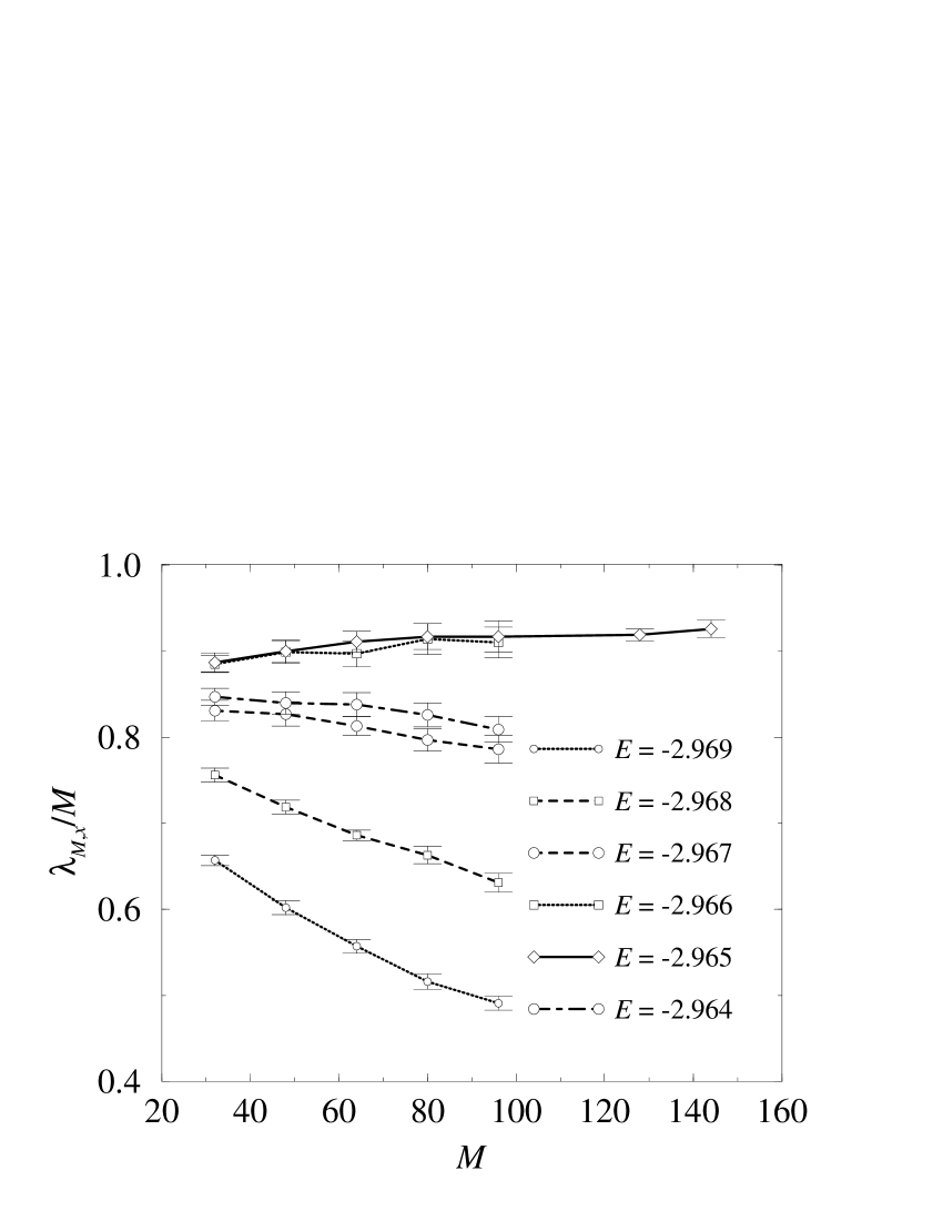
FIG. 1.: The critical values of the scaling functionns can be obtained from the large–$M$ limit of $\lambda_{M}/M$ at the critical energy. From the almost symmetrical behaviour of the values for the non–critical energies at either side of the critical one, we assume that the value for $E_{c}$ is between $-2.966$ and $-2.965$, but closer to the second one. Top: difficult hopping direction; bottom: easy hopping direction.

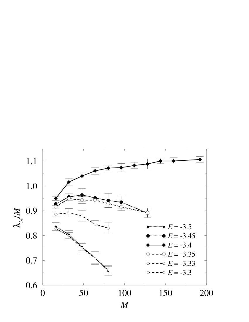
FIG. 2.: The critical value of the isotropic scaling function. From the large–$M$ data we estimate it to be $1.10\pm 0.03$.

FIG. 3.: The scaling functions for the difficult (open symbols) and easy (filled symbols) hopping directions $\lambda_{M}/M$ as a function of $\xi/M$. The localization lengths have been adjusted to better fit the data to a smooth curve. Energies are $-3.0$, $-2.99$, $-2.98$, $-2.97$, $-2.969$, $-2.968$, $-2.967$, $-2.964$, $-2.96$, $-2.95$, $-2.94$ and $-2.93$.

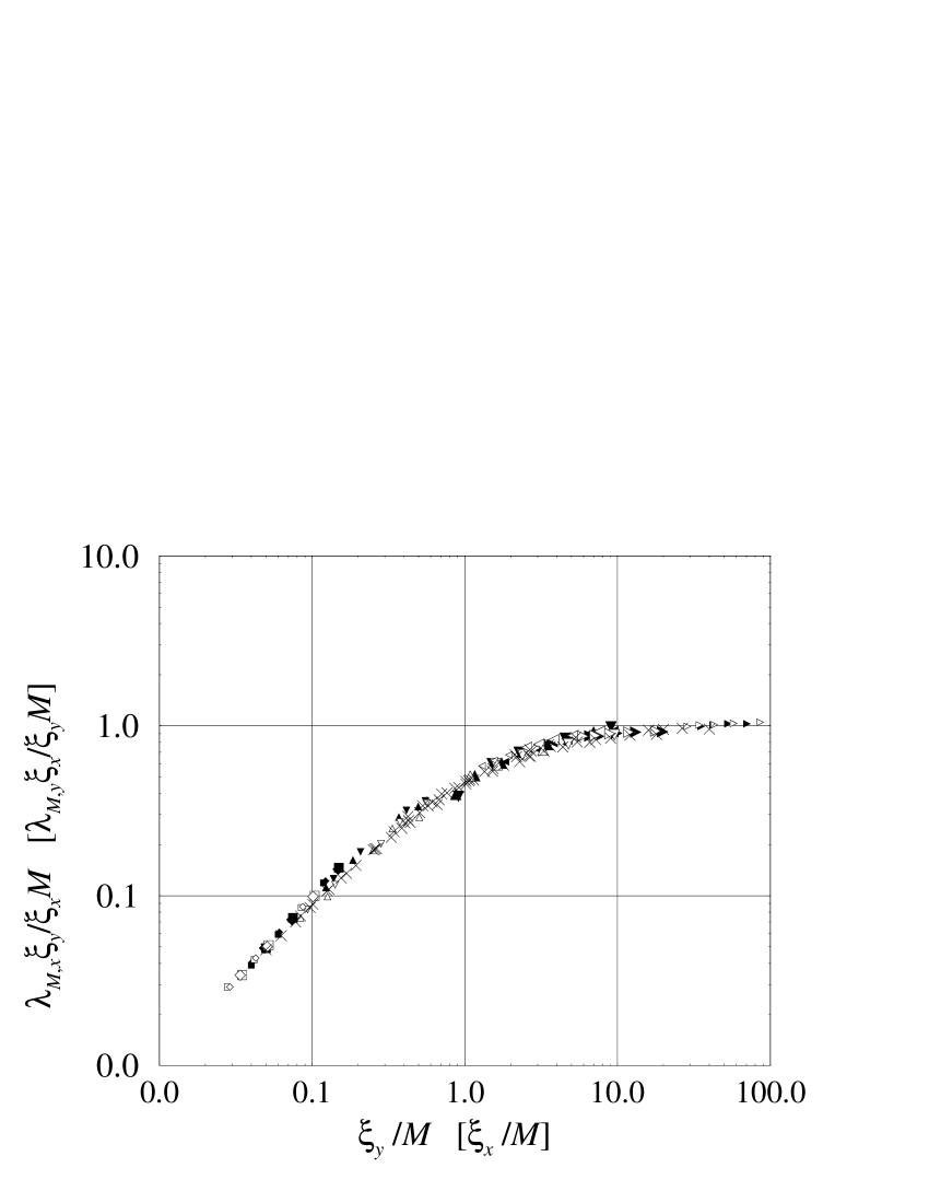
FIG. 4.: Plotting the rescaled scaling functions (cf. text) for the difficult (open symbols) and easy (filled symbols) hopping directions together with the scaling function for an isotropic system (crosses).

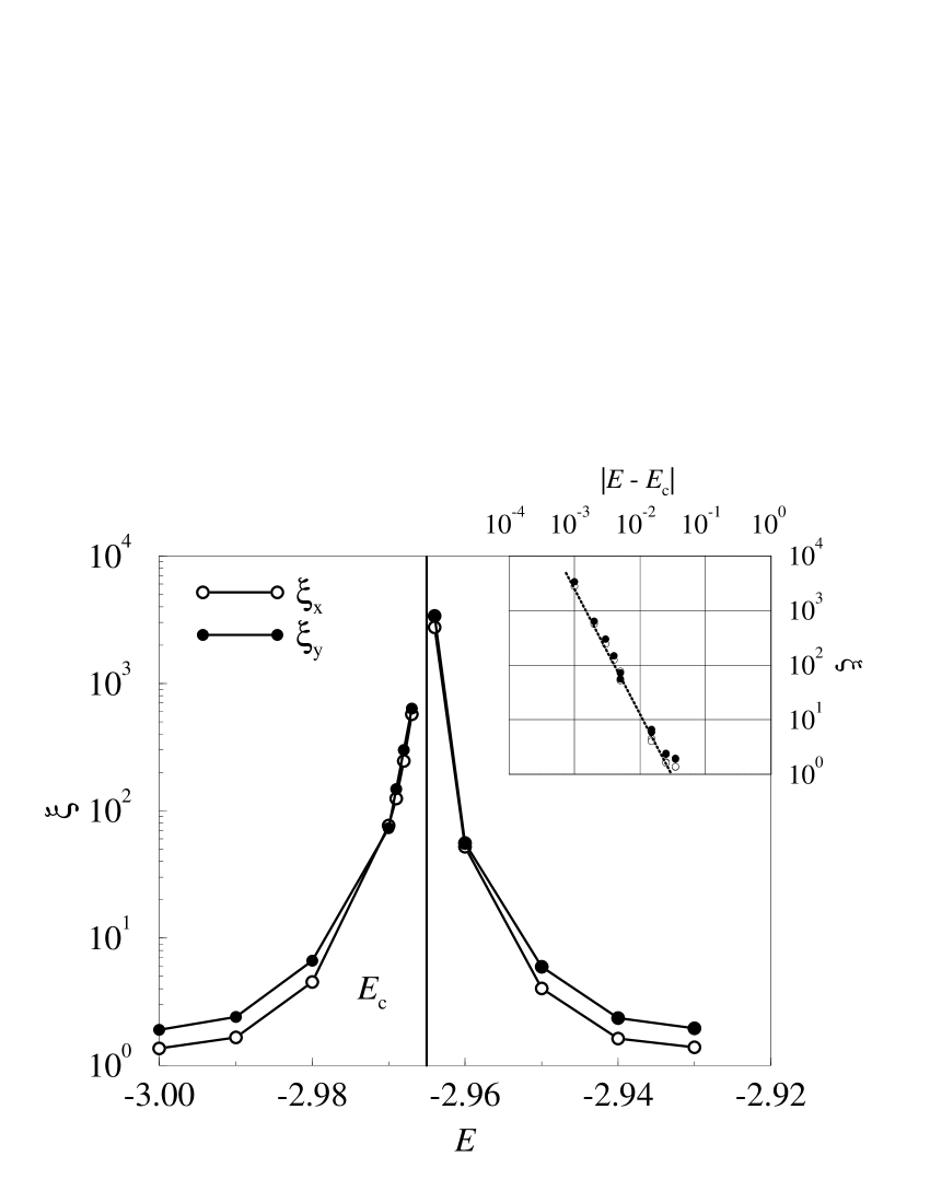
FIG. 5.: The divergence of the localization lengths at the critical Energy; open symbols: difficult hopping direction, filled symbols: easy hopping direction. The values are taken after the adjustments made to obtain Fig. 4. Inset: To extract the critical exponent of the localization lengths we plot $\xi$ vs $\left|E-E_{c}\right|$ in a log–log plot. Both exponents are found to be $2.3\pm 0.1$, roughly equal to the theoretical value for the isotropic system.

FIG. 6.: The density of states for the lowest subband for a disorder strength of $W=4.0$ (top) and $W=2.0$ (bottom), indicating that the critical energy is off the band center. A fit to a gaussian distribution suggests that the band center in the $W=2.0$ case is at $E_{0}\approx-3.38$, whereas the critical energy is $E_{c}\approx-3.32$.

REFERENCES

- [1] For a recent review, see B. Kramer, and A. McKinnon, Rep. Prog. Phys. 56, 1469 (1993).
- [2] Qiming Li, S. Katsoprinakis, E. N. Economou, and C. M. Soukoulis, Phys. Rev. B 56, R4297 (1997), and references therein.
- [3] F. Milde, R. A. Römer, and M. Schreiber, Phys. Rev. B 55, 9463 (1997).
- [4] I. Zambetaki, Q. Li, E. N Economou, and C. M. Soukoulis, Phys. Rev. Lett. 76, 3614 (1996); I. Zambetaki, Q. Li, E. N. Economou, and C. M. Soukoulis, Phys. Rev. B 56, 12221 (1997).
- [5] N. Dupuis, Phys. Rev. B 56, 9377 (1997); C. Mauz, A. Rosch, and P. Wölfle, Phys. Rev. B 56, 10953 (1997).
- [6] X. Wang, Ph. D. thesis at Iowa State University; X. Wang, Q. Li, and C. M. Soukoulis, unpublished.
- [7] S. Hikami, Prog. Theor. Phys. 63, 707 (1980).
- [8] For a review, see B. Huckestein, Rev. Mod. Phys. 67, 357 (1995).
- [9] A. Furusaki, Phys. Rev. Lett. 82, 604 (1999).
- [10] X. Wang, Q. Li, and C. M. Soukoulis, Phys. Rev. B 58, 3576 (1998).
- [11] J. K. Cullum, and R. A. Willoughby, Lanczos Algorithms for Large Symmetric Eigenvalue Computations, Birkhäuser, Boston, 1985, Progress in scientific computing ; v. 3.
- [12] O. Bohigas, and M.–J. Giannoni, Mathematical and Computational Methods in Nuclear Physics, pp. 1–99, Springer, New York, 1984, Lecture Notes in Physics ; v. 209.
- [13] M. L. Mehta, Random Matrices, Second edition, Academic Press, San Diego, 1991.
- [14] H. Potempa, A. Bäker, and L. Schweitzer, Physica A 256–258, 591 (1998).
- [15] H. Potempa, and L. Schweitzer, Ann. Phys. 7, 457 (1998).
- [16] M. Batsch, and L. Schweitzer, Proc. 12th Conf. High Magn. Fields in the Physics of Semicond. II, Würzburg 1996, World Scientific (1997), pp. 47–50.
- [17] M. Batsch, L. Schweitzer, and B. Kramer, Pysica B 249–251, 792 (1998).
- [18] R. Klesse, and M. Metzler, Phys. Rev. Lett. 79, 721 (1997).
- [19] J. T. Chalker, and P.D. coddington, J. Phys. C 21, 2665 (1988).
- [20] J. T. Chalker, V. E. Kravtsov, and I. V. Lerner, JETP Lett. 64, 386 (1996).
- [21] For an overview see M. Janßen, Int. J. Mod. Phys. B 8, 943 (1994).
- [22] W. Pook, and M. Janßen, Z. Phys. B 82, 295 (1991).
- [23] B. Huckestein, and R. Klesse, Phil. Mag. B 77 1181 (1998).
- [24] B. Huckestein, and L. Schweitzer, Proc. High Magnetic Fields in Semiconductor Physics III, Springer Series in Solid–State Sciences 101, Springer, pp. 84–88 (1992).
- [25] B. Huckestein, and L. Schweitzer, Phys. Rev. Lett. 72, 713 (1994).
- [26] B. Huckestein, Phys. Rev. Lett. 72, 1080 (1994).
- [27] D. H. Lee, Z. Wang, and S. Kivelson, Phys. Rev. Lett 70, 4130 (1993).