DISTRIBUTION OF RESONANCE WIDTHS IN LOCALIZED TIGHT-BINDING MODELS.

Marcello Terraneo (¹) and Italo Guarneri (²)
$({}^{1})$,$({}^{2})$ Dipartimento di Scienze Chimiche, Fisiche e Matematiche
Università dell’Insubria – Polo di Como
Via Lucini 3, I–22100 Como, Italy
$({}^{1})$, $({}^{2})$ Istituto Nazionale di Fisica della Materia, Unità di Milano, via Celoria 16, 20133 Milano, Italy
$({}^{2})$ and I.N.F.N., Sezione di Pavia, via Ugo Bassi 6, 27100 Pavia, Italy
$({}^{1})$ E-mail: Marcello.Terraneo@fisica.unimi.it
Preliminary Version as of

PACS: 47.52.+j; 72.10.-d; 72.15.Rn

Abstract

We numerically analyze the distribution of scattering resonance widths in one- and quasi-one dimensional tight binding models, in the localized regime. We detect and discuss an algebraic decay of the distribution, similar, though not identical, to recent theoretical predictions.

1 Introduction.

The decay in time of the survival probability inside open quantum systems is a nontrivial issue, both in Mesoscopic Physics and in Quantum Chaology. Such decay is determined by the distribution of resonance widths, which has been studied extensively[1].

Still, the effect of localization on the statistics of scattering resonances is not completely understood. In the strongly localized regime, some arguments [2] predict an asymptotic ${t^{-1}}$ law for the probability decay and a $\Gamma^{-1}$ behaviour for the distribution of resonance widths $\Gamma$; more recently, an analytical theory was developed [6], which slightly corrects the latter into an average decay $\Gamma^{-1.25}$.

In this paper we numerically address this question by investigating the $\Gamma$ distribution in a class of quasi-one dimensional models. Hamiltonians in this class are given by Band Random Matrices. As such matrices provide models for quantum localization not only in disordered solids but in chaotic Hamiltonian systems, too [3], our present results are also relevant to the latter class of problems [7].

We use a computational scheme based on the Effective Hamiltonian (EH) approach: however, at variance with the usual way of implementing EHs, which neglects their energy dependence, we perform an exact (within the limits of numerical accuracy) computation of the distribution. Our method is described in sec. 2. In this way we indeed detect a large interval of $\Gamma$ in which $P(\Gamma)$ decays like $\Gamma^{-\alpha}$ with $\alpha$ in the range $1-2$, depending on the model, and on the localization ratio. Our results therefore signal algebraic decay, still somewhat different from the predictions of ref.[6]. Some other differences appear, in the large-${\Gamma}$ part of the distribution.

However, comparing numerical results with theoretical predictions is by no means an obvious task. First, the theory of ref.[6] is one for a continuous model, while our models are discrete. Second, that theory somehow assumes a certain ideal coupling to continuum, different from ours. Finally, the large-size asymptotic regime in this problem has some nontrivial features, which impose caution in analyzing finite-sample data.

In sec.3 we discuss some general features of the problem, based on general facts about Anderson localization, and on elementary mathematical estimates which we derive for our class of discrete models, and which are well confirmed by our data. Our numerical results are described and discussed in the conclusive sec. 4.

2 Models, and Effective Hamiltonians.

We consider one-dimensional lattice Hamiltonians, which describe a wire coupled to one or two perfect leads, in the form:

$$H=H^{(i)}+H^{(o)}+H^{(io)}$$ (1)

The first two terms describe the wire and the leads, respectively; the third term describes the coupling between them. We label lattice sites by an integer $j$, in such a way that the wire is described by $1\leq j\leq N$. The Hamiltonian in the leads describes hopping between sites spaced by a fixed integer $b$; in the basis of vectors $|j\rangle$, it has nonzero matrix elements only between sites $i,j$ which belong in the same lead, that is, they are both larger than $N$ or smaller than $1$. In that case,

$$H^{(o)}_{ij}=\delta_{i,j+b}+\delta_{i,j-b}$$ (2)

The wire Hamiltonian is a finite, $N\times N$ matrix with nonzero elements only between sites within the wire. Finally, the operator $H^{(io)}$ couples sites $i,j$ spaced by $b$, one lying in the wire and the other in a lead. The corresponding matrix elements again have the form (2).

We have considered two special cases, namely:

(i) $b=1$, $H^{(i)}$ a tridiagonal matrix with unit off-diagonal elements and diagonal elements given by independent random variables uniformly distributed in the interval $[-W/2,+W/2]$. This is a finite sample of a one-dimensional Anderson model coupled to leads on both sides. In the discussion below we shall also make reference to the one-sided Anderson model, in which the Hamiltonian matrix is a semi-infinite rather than a doubly infinite one. This is equivalent to inserting a perfectly reflecting boundary at $n=N+1$.

(ii) $N>b>1$, the wire Hamiltonian is a Band Random Matrix (BRM), that is, a real symmetric matrix of rank $N$ such that $H_{i,j}\neq 0\leftrightarrow|i-j|\leq b$. $H_{i,j}^{(i)}$ are independent Gaussian variables, with variance $\frac{\beta^{2}}{2}$ for off-diagonal elements and $\beta^{2}$ for diagonal ones. We have chosen $\beta=1$. As analyzed in [4], this corresponds to the “matching wire” regime discussed by Ekonomou and Soukolis [5].

In both cases (i),(ii) the Schroedinger equation for free propagation in the leads has solutions $u_{m}=\frac{1}{\sqrt{2\pi}}e^{ikm}$, with dispersion law $E=2\cos kb$. For any energy value $E$ in the interval $[-2,2]$ there are $b$ different allowed momenta,

$$k_{s}=\frac{\arccos{\frac{E}{2}}}{b}+\frac{2\pi}{b}s$$ (3)

with $s=0\ldots b-1$. There are $b$ incoming and $b$ outgoing waves, hence the wire enforces multichannel scattering. It is important to remark that with the choice (2) the velocity $v_{i}=\frac{dH}{dk_{i}}|_{H=E}$ is the same in all channels.

The S-matrix relates amplitudes of incoming and outgoing plane waves, $I_{L,R}$ and $O_{L,R}$ respectively ($L$ and $R$ stand for left and right):

$$S\left(\matrix{I_{L}\cr I_{R}}\right)=\left(\matrix{O_{L}\cr O_{R}}\right)$$

In our representation, the S-matrix is a $2b\times 2b$ energy-dependent matrix $S_{s,l}(E)$, where $l$, $s$ are channel indexes.

We compute the scattering matrix from the Lippman-Schwinger equation for the scattering states

$$u^{\pm}-G_{0}^{\pm}\cdot Vu^{\pm}=u$$ (4)

where $u$ are the free eigenfunctions, $u^{\pm}$ the scattering states and V is the “potential”: a matrix of rank N defined via the formula $H-H_{0}=V$. $G_{0}^{\pm}$ is the free Green function $G_{0}^{\pm}=(E\pm i\epsilon-H_{0})^{-1}$. It can be computed by a complex integral:

$$(G_{0}^{\pm})_{n,m} =\langle n|(E-H_{0}{\pm}i\epsilon)^{-1}|m\rangle\big{|}_{\epsilon=0} ={1\over{2\pi}}\int_{0}^{2\pi}dk{e^{i(m-n)k}\over{E{\pm}i\epsilon-{2\cos{kb}}}}\Bigg{|}_{\epsilon=0}$$ (5)

The scattering matrix is given by:

$$S_{ij}=\delta_{ij}-2\pi i\sqrt{{dk_{i}\over dH}}\Bigg{|}_{H=E}\sqrt{{dk_{j}\over dH}}\Bigg{|}_{H=E}<u_{i}\left|V\right|u_{j}^{\pm}>$$ (6)

where $i$, $j$ are channel labels, and $\sqrt{{dk_{i}\over dH}}\Bigg{|}_{H=E}$ is the density of states in channel $i$.

Now, $G^{0}$ can be written in block form as

$$\left[\matrix{g_{11}^{0}&g_{12}^{0}&g_{13}^{0}\cr g_{21}^{0}&g_{22}^{0}&g_{23}^{0}\cr g_{31}^{0}&g_{32}^{0}&g_{33}^{0}}\right]$$

In this section we use small letters for blocks (i.e, submatrices) and capital letters for full operators. Here $g_{11}^{0}$, $g_{33}^{0}$, $g_{31}^{0}$ and $g_{13}^{0}$ are semi-infinite matrices, $g_{22}^{0}$ is a $N\times N$ matrix, $g_{12}^{0}$ and $g_{32}^{0}$ are matrices with $N$ columns and infinitely many rows, $g_{21}^{0}$ and $g_{23}^{0}$ have $N$ rows and infinitely many columns. As the potential matrix is localized within the center block (2,2), we write it in the block form

$$\left[\matrix{0&0&0\cr 0&v&0\cr 0&0&0}\right]$$

The poles of the S-matrix are the complex values of energy for which the $N\times N$ matrix $(I-g_{22}^{0\pm}v)$ has no inverse; hence, they are given by the roots of

$$det(I-g_{22}^{0\pm}v)=0$$ (7)

In order to solve this equation we introduce an ’effective Hamiltonian’ matrix $H_{eff}$ of rank N. This is a well known construction [8], [9], [10], but the exact form of the effective hamiltonian for our specific models is not immediately derived from the general theory. There are in fact certain slight differencies between our effective Hamiltonian and the one used in [6], which are probably due to a different choice of the Hamiltonian in the leads. Therefore we shall presently give a complete derivation for our specific models.

We start with the identity

$$G_{0}=G-G_{0}VG=(1-G_{0}V)G.$$ (8)

where $G=(E\pm i\epsilon-H)^{-1}|_{\epsilon=0}$ Multiplying on the left by $G_{0}^{-1}$ and on the right by $G^{-1}$, we have

$$G^{-1}=G_{0}^{-1}-V.$$

The block form of (8) is

$$\left[\matrix{g^{0}_{11}&g^{0}_{12}&g^{0}_{13}\cr g^{0}_{21}&g^{0}_{22}&g^{0}_{23}\cr g^{0}_{31}&g^{0}_{32}&g^{0}_{33}}\right]=\left[\matrix{1&-g^{0}_{12}v&0\cr 0&(1-g^{0}_{22}v)&0\cr 0&-g^{0}_{32}v&1}\right]\left[\matrix{g_{11}&g_{12}&g_{13}\cr g_{21}&g_{22}&g_{23}\cr g_{31}&g_{32}&g_{33}}\right]$$

where $1$ and $0$ are identity and zero matrices of dimensions corresponding to their position in the infinite matrix.

For the center block we have $g_{22}^{0}=(1-g_{22}^{0}v)g_{22}$, whence, multiplying on the left by ${g_{22}^{0}}^{-1}$ and on the right by $g_{22}^{-1}$, we obtain

$$g_{22}^{-1}=({g_{22}^{0}}^{-1}-v).$$ (9)

In order to compute $(g_{22}^{0})^{-1}$ we start from the definition, which in block forms reads

$$\left[\matrix{g^{0}_{11}&g^{0}_{12}&g^{0}_{13}\cr g^{0}_{21}&g^{0}_{22}&g^{0}_{23}\cr g^{0}_{31}&g^{0}_{32}&g^{0}_{33}}\right]\left[\matrix{E-h^{0}_{11}&u_{12}&0\cr u_{21}&E-h^{0}_{22}&u_{23}\cr 0&u_{32}&E-h^{0}_{33}}\right]=\left[\matrix{1&0&0\cr 0&1&0\cr 0&0&1}\right]$$

where $u_{ij}=-h^{0}_{ij}$ are the coupling matrices.

The equation for the center block is

$$g^{0}_{21}u_{12}+g^{0}_{22}(E-h^{0}_{22})+g^{0}_{23}u_{32}=1.$$ (10)

From (5) we know that the free Green function is a Toeplitz matrix, whose center block $g^{0}_{22}$ can be written:

$$\left[\matrix{x_{0}&x_{1}&\ldots&x_{N-1}\cr x_{1}&\ddots&\ddots&\vdots\cr\vdots&\ddots&\ddots&x_{1}\cr x_{N-1}&\ldots&x_{1}&x_{0}}\right]$$

where $x_{s}=0$ if $s$ is not a multiple of $b$, while, if $s=lb$, then $x_{lb}=x_{0}e^{ilk}$, with $k=\arccos{(\frac{E}{2})}$. Keeping this in mind we get

$$(g^{0}_{21}u_{12}+g^{0}_{23}u_{32})=\left[\matrix{x_{b}&\ldots&x_{1}&0&\ldots&0&x_{N+1}&\ldots&x_{N+b}\cr\vdots&&\vdots&\vdots&&\vdots&\vdots&&\vdots\cr x_{N+b}&\ldots&x_{N+1}&0&\ldots&0&x_{1}&\ldots&x_{b}}\right]=-g^{0}_{22}\cdot K_{b}.$$

where $K_{b}=diag(e^{ikb},\ldots,e^{ikb},0,\ldots,0,e^{ikb},\ldots,e^{ikb})$ is the “self-energy”.

Then from (10) we obtain:

$$(g^{0}_{22})^{-1}=(E-h^{0}_{22}-K_{b}).$$

Finally, (9) yields:

$$(g_{22})^{-1}=(g^{0}_{22})^{-1}-v=(E-h^{0}_{22}-K_{b}-v)=(E-h_{22}-K_{b}(E))=(E-H_{eff}(E)).$$

where $H_{eff}(E)=h_{22}+K_{b}(E)$ is the effective Hamiltonian matrix of rank $N$. The role of the effective Hamiltonian emerges on noting that:

$$I-g^{0}_{22}v=g^{0}_{22}((g^{0}_{22})^{-1}-v)=g^{0}_{22}(E-H_{eff}(E))$$

which shows that solving eqn.(7) is the same as solving the equation:

$$det(H_{eff}(E)-E)=0$$ (11)

For further use we rewrite $H_{eff}$ in operator notation. In place of $h_{22}$ we rewrite $H^{(i)}$: the Hamiltonian operator of the sample, with Dirichlet conditions at $n=0$ and $n=N+1$. Then

$$H_{eff}(E)=H^{(i)}+e^{ik(E)b}\left\{\sum\limits_{n=1}^{b}+\sum\limits_{n=N-b+1}^{N}\right\}|n\rangle\langle n|$$ (12)

The leads only affect diagonal elements, at sites near the contact points. For the Anderson model, where hopping only occurs between neighbouring sites, only the first and the last diagonal elements of the Hamiltonian are affected. Some straightforward modifications to the above construction are necessary in the one-sided Anderson case; we omit details here.

Solving the nonlinear eqn.(11) is a difficult task. When using the effective hamiltonian formalism, one typically neglects the dependence of $H_{eff}$ on energy, so the problem is reduced to finding eigenvalues of the effective hamiltonian at a chosen fixed value $E_{0}$ of the energy. Such eigenvalues depend on $E_{0}$ as a parameter; for convenience of language, we will term them parametric resonances in the following, reserving the name exact resonances to solutions of eqn.(11).

3 Theoretical Premises.

A few remarks are in order, about the mathematical problem set by the above formalism. These are most simply formulated for the one-sided Anderson case, so we restrict to that case; nevertheless, similar arguments can be developed for the two-sided Anderson and for the band matrix models.

If $E$ is a root of eqn.(11), then there is a vector $|\psi\rangle$ of unit norm, satisfying the equation:

$$H^{(i)}|\psi\rangle+e^{ik(E)}|1\rangle\langle 1|\psi\rangle=E|\psi\rangle$$ (13)

where $H^{(i)}$ is now the Anderson Hamiltonian with Dirichlet boundary conditions at $n=0$, $n=N+1$. Multiplying eqn.(13) on the left by $\psi$, and taking imaginary parts, we get:

$${\cal I}m(e^{ik(E)})|\langle 1|\psi\rangle|^{2}=\Gamma$$ (14)

where we have set $E=x+i\Gamma$ with real $x,\Gamma$.

From the dispersion law the following analytical expression of $e^{ik(E)}$ follows:

$$e^{ik(E)}=\frac{E+\sqrt{E^{2}-4}}{2}$$ (15)

In the physical sheet, the square root in eqn.(15) has to be chosen such that its imaginary part is opposite in sign to $\Gamma={\cal I}m(E)$; then an easy computation shows that ${\cal I}m(e^{ik(E)})$ is opposite in sign to $\Gamma$, so eqn.(14) cannot have solutions with $\Gamma\neq 0$. In order to solve it, we have to continue $H_{eff}$ into the nonphysical sheet, across the branch cut $[-2,+2]$.

We now address the problem of finding estimates for the largest $\Gamma$. We consider parametric resonances first: if $E_{0}$ is chosen in $(-2,2)$, then eqn.(14) immediately sets a sharp, realization-independent bound on parametric $\Gamma$:

$$|\Gamma|\leq|\sin(k(E_{0}))|=\frac{\sqrt{4-E_{0}^{2}}}{2}\leq 1$$ (16)

For exact resonances we can only establish a milder, realization-dependent bound. Multiplying eqn.(13) on the left by $\langle 1|$, using eqn.(13), and the explicit form of $H^{(i)}$, we get:

$$\langle 2|\psi\rangle=\langle 1|\psi\rangle\left(E-e^{ik(E)}-V(1)\right)$$ (17)

where $V(1)$ is the random on-site potential at site $1$. Since $|\langle 2|\psi\rangle|^{2}+|\langle 1|\psi\rangle|^{2}\leq 1$, using eqn.(13) we get the inequality:

$$\frac{\Gamma}{{\cal I}m(e^{ik(E)})}\leq\frac{1}{1+|E-e^{ik(E)}-V(1)|^{2}}$$ (18)

which, given a realization of the random potential, sets an upper bound to ${\Gamma}$. At the center of the spectrum and small $V(1)$ this bound has approximately the form $|\Gamma|\leq|V(1)|^{-1}$. In turn, this implies that those realizations of the random potential which yield $\Gamma$’s larger than a given $\gamma$ have a probability not larger than $\sim 1/\gamma$. This bound on the large-$\Gamma$ behaviour of the $P(\Gamma)$ distribution of exact resonances is much milder than the bound (16) for parametric resonances. We anticipate that this difference is manifest in numerical data (see fig.4, 5 and 6)

In the limit $N=\infty$, both $H^{(i)}$ and $H_{eff}(E_{0})$ become operators in $\infty-$ dimensional Hilbert space. The latter operator is obtained by adding a rank-one perturbation to the former, which in turn has a dense point spectrum in the interval $I=[-W/2-2,+W/2+2]$ (with probability 1). From general operator theory it follows, that in the limit $N=\infty$ the distribution of parametric $\Gamma$’s collapses into a Dirac delta at zero - unlike other scattering statistics, (e.g., the phase shift distribution), which have a smooth limit distribution. This physically intuitive result should be valid for the distribution of exact resonances, too.

Thus, on increasing $N$, we should expect the leftmost part of the finite-$N$ distribution $P(\Gamma)$ to rise, and the rest to gradually subside. To further illustrate this point, we reformulate eqn.(13) by projecting it onto the basis of eigenvectors $u_{n}$ of $H^{(i)}$. Denoting $E_{n}$ the corresponding eigenvalues and $\psi_{n}$ the amplitudes of $\psi$, we get:

$$\psi_{n}=-\frac{e^{ik(E)}\langle u_{n}|1\rangle\langle 1|\psi\rangle}{E_{n}-E}$$

whence:

$$\langle 1|\psi\rangle=-\langle 1|\psi\rangle e^{ik(E)}\frac{|\langle u_{n}|1\rangle|^{2}}{E_{n}-E}$$

As $\langle 1|\psi\rangle=0$ is excluded, the resonant values of $E$ must solve the key equation:

$$\sum\limits_{n}\frac{p_{n}}{E_{n}-E}=-e^{-ik(E)}$$ (19)

where $p_{n}=|\langle 1|u_{n}\rangle|^{2}$.

At large $N$, the eigenfunctions $u_{n}$ are exponentially localized, with localization lenghts $\xi(E_{n})$. For resonances $E=x+i\Gamma$ with $|\Gamma|\ll 1/N$, a single-pole approximation to the lhs of eqn.(19) should be valid, because eigenfunctions with $E_{n}$’s much closer than the average level spacing typically have an exponentially small overlap; so the sum in (19) is dominated by a single term[11]. Hence, the narrowest resonances can be assumed to solve

$$p_{n}e^{ik(E)}\approx(E-E_{n})$$

with $p_{n}$ small, so

$$E\approx E_{n}+p_{n}e^{ik(E_{n})},~{}~{}\mbox{\rm and}~{}~{}\Gamma\approx p_{n}\sin(k(E_{n})).$$ (20)

If we further restrict near the center of the spectrum, then the smallest $\Gamma$ come from states $u_{n}$ localized around sites $n_{0}(n)$ lying in the rightmost part of the sample. For these, $\log(p_{n})\approx-2n_{0}(n)/\xi+\eta_{n}$, with $\xi$ the localization length at the band center and $\eta_{n}$ a fluctuating quantity of order $\sqrt{n}_{0}$.

Thus the distribution of very small $\Gamma$’s is ruled by the distribution of $p_{n}$’s. If in addition $\Gamma\ll\exp(-2N/\xi)$, the latter distribution is mainly determined by fluctuations of $\eta_{n}$; assuming a gaussian distribution for the latter, one gets that in this region $P(\Gamma)$ has the lognormal distribution already well known in this context. Nevertheless, this part becomes negligible at large $N$, because it comes of a fraction $\sim\xi/N$ of the full set of all resonances.

Away from this extreme region, the $\Gamma$ statistics is more and more affected by the change in $n_{0}$. Neglecting $\eta_{n}$ completely, one deduces a dependence $\sim 1/\Gamma$, by a simple argument already reproduced in ref.[6]. The presence of $\eta_{n}$ just smoothens the cusp of $1/\Gamma$ at $\Gamma\approx\exp(-2N/\xi)$, but the $1/\Gamma$ law again re-emerges at larger $\Gamma$.

So finite-N, normalized distributions $P(\Gamma)$ have a peak at $\sim\exp(-2N/\xi)$, of height $\sim\exp(2N/\xi)$. It is this very peak which eventually builds the limit $\delta-$ distribution. In the range $\exp(-2N/\xi)<\Gamma\ll 1/N$, the above rough argument suggests a law $\sim 1/\Gamma$; but it must be mentioned that according to Titov and Fyodorov ([6]) this inverse law should be restricted to a smaller range. Some numerical data about this issue will be given in the next section.

The large $\Gamma$ region is essentially determined by the coupling to continuum, so it should be model-dependent. Nevertheless, it is reasonable to assume that the number of resonances involved is constant, of order $\xi$; if so, again this tail should subside at large $N$, at the rate $\sim\xi/N$.

Finally we use eqn.(19) to investigate the reliability of parametric resonances as approximations of exact ones. The equation for parametric resonances is obtained from eqn.(19) by replacing in the rhs $E$ by a fixed $E_{0}$ chosen in $(-2,+2)$. An obvious requirement for parametric resonances to approximate exact ones is that their dependence on $E_{0}$ be mild. Now,

$$\left|\frac{dE}{dE_{0}}\right|=\left|\sum\limits_{n}\frac{|\langle u_{n}|1\rangle|^{2}}{(E_{n}-E)^{2}}\right|^{-1}\left|\frac{dk(E_{0})}{dE_{0}}\right|\geq\frac{\Gamma^{2}}{\sqrt{4-E_{0}^{2}}}$$

If a given parametric resonance is to vary little on changing $E_{0}$ on the order of its width $\Gamma$, it is therefore necessary that:

$$\Gamma^{2}\ll{\sqrt{4-E_{0}^{2}}}$$

which shows that the parametric approximation becomes unreliable close to the edges $\pm 2$, and in any case at $\Gamma\sim 1$.

4 Numerical Method, and Results.

As we are only interested in the statistical distribution of the imaginary parts of solutions of (11), we don’t need to compute them exactly. Instead, we use the fact that the number of zeros of an analytic function $f(z)$ inside a closed path is equal to the variation of the phase of the function itself along the path divided by $2\pi$. We have therefore considered rectangular regions $\{E:|Re(E)|\leq E_{0},-\gamma\leq Im(E)\leq 0\}$ in the lower part of the 2nd Riemann sheet. By numerically computing the phase of $det(H_{eff}-E)$ along the boundaries of such regions we obtained $N(\gamma,E_{0})$, the number of resonances having real parts in $(-E_{0},+E_{0})$, and widths not larger than $\gamma$. Typically $E_{0}=0.5$ in our computations.

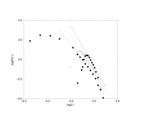
Figure 1: P($\Gamma$) for BRM model

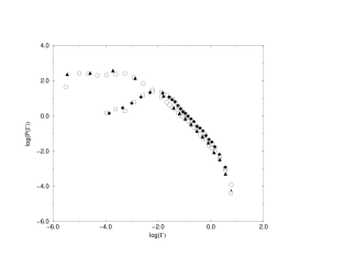
Figure 2: P($\Gamma$) for BRM model

Repeating the procedure for different realizations of our random Hamiltonians, we obtained the histograms of resonance widths shown in Figs. 1 - 6 (there $P(\Gamma)$ is the probability density for $\Gamma$ values). The numerical procedure is quite heavy, so we were able to process at most $400$ realizations of the BRM model. With the Anderson model, computation is faster, so we could process up to $1000$ realizations.

Most of the distributions of resonance widths $P(\Gamma)$ computed by the above discussed method decay, at very large $\Gamma$, faster than power-like, also because of the difficulty of numerically building good statistics in this poorly populated region.

However, in an intermediate region of values of $\Gamma$, the observed decay is algebraic, proportional to $\Gamma^{-\alpha}$. The width of this region depends on the localization ratio $r$, which is proportional to $b^{2}/N$ and to $1/(NW^{2})$ for the BRM model and for the Anderson model respectively. The region of algebraic decay is very broad in strong localized systems, $r\ll 1$; it shrinks as $r$ is increased, and eventually disappears in the metallic region $r\gg 1$.

The behaviour of the exponent $\alpha$ is somewhat different in the BRM and in the Anderson model. In the former case, $\alpha$ increases as $r$ increases, going from values about $1.5-1.6$ to values about $2-2.1$ (see fig.1). Data obtained at fixed $r$ and different values of $N$, $b$ ( with $\frac{N}{b}\geq 5$, though) show that $\alpha$ only depends on the localization ratio in the explored parameter range: see fig. 2, which shows distributions with approximately the same localization ratios and different $N$, $b$.

We have numerically computed distributions of widths for the one and two-leads Anderson model, too, by solving eqn.(11) as explained above. In this case, $\alpha$ remains more or less constant around $1.7-1.8$: it doesn’t seem to depend on the localization ratio (fig. 3) in the explored parameter range. The only effect of decreasing $W$ is the predicted shift of the peak of the distribution towards larger values $\Gamma$.

Most of our data do not yet pertain to the true asymptotic large-$N$ regime. In fact, the peak in the left-hand part of our data is still relatively broad in comparison to the right-hand part, so the asymptotically interesting region $e^{-2N/{\xi}}\ll\Gamma\ll 1$ is still somewhat restricted. Nevertheless the region of algebraic decay is already clean, and relatively stable against variation of the localization ratio. We therefore surmise, that in more localized regimes the local exponent $\alpha$ would be found to smoothly decrease with $\Gamma$, tending to $1$ as the peak of the distribution is approached from the right. As we shall presently discuss, we get indications in this sense from distributions of parametric $\Gamma$’s, whose computation could be pushed to significantly more localized situations than accessible to exact computations, based on solving eqn.(11).

Parametric distributions were obtained by diagonalizing $H_{eff}(0)$. Both for the BRM and the Anderson model, they exhibit a cut-off at $\Gamma\sim 1$ which is absent in the real distributions. The latter in fact decays to zero much more gently. In other words: in all the models we have studied, neglecting the energy dependence of effective Hamiltonians yields acceptable results only at resonance widths appreciably smaller than $1$ (figs. 4, 5 and 6). The reason is that, at such large widths, the effective hamiltonian is significantly changing already over the width of single resonances. These numerical findings are fully consistent with the analysis in section 3.

Exact and parametric distributions fairly well agree in the central part, on the right of the peak, but they are again somewhat different on the left. The reason is probably that our exact distributions collect resonances from a relatively broad interval of real energies, so they include resonances closer to the edges, where smaller $\Gamma$’s are a priori expected (eqn.(20)).

The sharp cut-off of numerical distributions of parametric resonances was also observed in ref.[6], and found to be consistent with the therein developed theory for exact resonances in a continuous, white-noise model. That coincidence between exact and parametric distributions at relatively large $\Gamma$ raises an interesting theoretical problem about the role of the coupling.[12]

In fig.4 we compare parametric and exact distributions both for the one- and the two-sided Anderson model. Note that one-lead data refer to a significantly more localized regime than two-lead ones, and yield smaller $\alpha$’s. The estimated $\alpha$ for one-sided Anderson is in this case $\approx 1.1$. In fig.5 we have again computed the parametric distribution for one-sided Anderson, this time in an even more localized situation. Moving from left to right, the lhs part of the distribution now exhibits $\alpha\approx 1$ over three decades, after which the distribution gradually drops to zero in roughly two decades.

We finally note that the rightmost part of the exact distribution in fig.5 is well fitted by a $\Gamma^{-2}$ law. As the latter coincides with the upper bound established in sec.3 for exact resonances, we have an indication that that bound is probably optimal.

In summary: in this paper we have analyzed the distributions of imaginary parts of resonances in different tight-binding models. The most interesting result is the presence of a region with power like decay, both for Anderson and BRM model. It was obtained by numerically implementing the effective Hamiltonian method, in a way which doesn’t a priori neglect energy dependence. Our analysis indicates that most of the distribution of widths tends to concentrate within a single peak around $\Gamma\sim\exp(-2N/{\xi})$ as more and more localized regimes are approached. While subsiding (with increasing $N$), the distribution of widths on the right of the peak displays an algebraic dependence on $\Gamma$. The related exponent ranges from $1$ (at small $\Gamma$), to $2$ (at large $\Gamma$). In the latter region, however, the specific form of the coupling to continuum plays a role.

Useful discussions with G.Maspero are acknowledged. We are grateful to Y.Fyodorov and M.Titov for communicating us unpublished details of their work.

Figure 1: Distribution of exact resonance widths for BRM models with different localization ratios. Diamonds: $N=100$, bandwidth $5$, the slope of the dashed line is $-1.6$. Squares: $N=150$, bandwidth $26$, the slope of the solid line is $-2.1$. Crosses: $N=200$, bandwidth $20$, slope $-1.85$.

Figure 2: Distribution of exact resonance widths for BRM models with similar localization ratios. Diamonds: $N=150$, bandwidth $10$. Squares: $N=200$, bandwidth $12$. Circles: $N=200$, bandwidth $7$. Triangles: $N=150$, bandwidth $6$. Their localization ratios $\frac{b^{2}}{N}$ are $0.67,0.72,0.245,0.24$, respectively.

Figure 3: Distribution of exact resonance widths for the two-leads Anderson model, with different localization ratios. Diamonds: $N=150$, $W=1.1$. Circles: $N=100$, $W=1.5$. Crosses: $N=100$, $W=0.3$. The slope of the line is $-1.75$.

Figure 4: Distribution of parametric and exact resonance widths for the Anderson model. Diamonds: exact resonances at $N=100$, $W=2.5$, one lead. Squares: exact resonances at $N=100$, $W=1.5$, two leads. The dashed and the solid lines represent parametric resonances obtained by diagonalizing $H_{eff}(0)$, for 1- and 2- leads model, respectively.

Figure 5 Distribution of parametric and exact resonance widths for the one-lead Anderson model. Squares: parametric resonances at $N=300$, $W=2$. The slope of the main straight line is $-1$, that of the shorter one on the right is $-2$. Diamonds are reproduced from Fig.4, which refers to a less localized situation.

Figure 6: Distribution of parametric and exact resonance widths for the BRM model. Diamonds: $N=100$, bandwidth $15$. Circles: $N=100$, bandwidth $5$. Triangles, $N=150$, bandwith $10$. The curves represent parametric resonances obtained by diagonalizing $H_{eff}(0)$.

Figure 3: P($\Gamma$) for the Anderson model

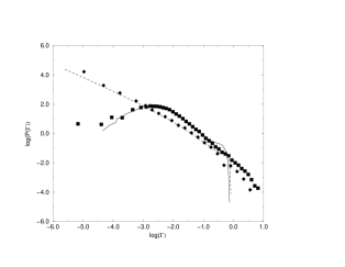
Figure 4: P($\Gamma$) for the Anderson model

Figure 5: P($\Gamma$) for the 1-lead Anderson model

Figure 6: P($\Gamma$) for BRM model

References

- [1] Y.V.Fyodorov and H.-J. Sommers, J.Math.Phys. 38, (1997) 1918
- [2] G.Casati, G.Maspero and D.Shepelyansky, Phys. Rev. Lett., 82, (1999) 524.
- [3] G.Casati, B.Chirikov, I.Guarneri, F.Izrailev, Phys. Rev. E 48, (1993), R1613.
- [4] G.Casati,I.Guarneri and G.Maspero, J.Phys.I 7, (1997), 729-736
- [5] E.N. Economou and C.M. Soukolis,Phys.Rev.Lett. 43, (1981), 618
- [6] M.Titov and Y.V.Fyodorov , Phys. Rev. B, 61, (2000), 2444.
- [7] Indications in this sense have been found by G.Maspero, who has detected an algebraic tail with a dynamical model with localization ratio (private communication).
- [8] Verbaarschot et al., Phys.Rep. 129, (1985),367.
- [9] T.Guhr et al., Phys. Rep. 299, (1998),189.
- [10] C.Beenakker, Rev.Mod.Phys. 69, (1997), 189.
- [11] We note in passing that the single-pole approximation is never valid at .
- [12] The parametric distributions of ref.([6]) were obtained by diagonalizing an effective Hamiltonian, which simulates coupling to continuum by adding an imaginary shift to the last diagonal element. That marks a difference with our computations, which (of necessity) have a shift instead. Distributions computed that way are different from ours in the right hand tails - for instance, they exhibit an isolated group of resonances beyond the cutoff, at - but are quite similar at small .