Hierarchical learning in polynomial Support Vector
Machines

Abstract

We study the typical properties of polynomial Support Vector Machines within a Statistical Mechanics approach that allows us to analyze the effect of different normalizations of the features. If the normalization is adecuately chosen, there is a hierarchical learning of features of increasing order as a function of the training set size.

guessConjecture

1 Introduction

The theoretical basis of learning from examples relies on the possibility of bounding the generalization error, which is the probability that the trained machine makes an error on a new pattern. However, the rigorous bounds deduced with methods of statistical theory [Vapnik (1995)], which hold for the worst case, turn out to be too pessimistic in most real world applications. Bounds to the estimator of the generalization error, obtained by the leave-one-out technique, are closer to experimental results [Vapnik and Chapelle (2000)]. This estimator is obtained through averaging the classification error on one pattern, when learning was achieved by removing that pattern from the training set. Another approach to learning theory, heralded more than a decade ago by the pioneering work of E. Gardner on perceptrons [Gardner and Derrida (1988)], strives to determine analytically the typical properties of the learning machine under somewhat restrictive hypothesis. This is done using methods from Statistical Physics, developed to study the properties of large, disordered physical systems. The basic assumption of this approach is that average quantities are representative of the machine’s properties, with a probability that tends to the unity as the system’s size goes to infinity, a limit usually called the thermodynamic (TD) limit. Thus, in this limit, the leave-one-out estimators and the Statistical Mechanics results are expected to converge to the same values. The input patterns distribution plays the role of the disorder over which averages are taken, the size of the system being the input space dimension. In the TD limit, some control parameters, like the training set size relative to the input space dimension, are kept fixed. This enables to deduce typical properties for small relative training set sizes, in contrast to the bounds provided by the statistical theories, which are generally valid for sufficiently large training sets. In this paper we are able to get deeper insight on the typical properties of Support Vector Machines (SVMs) by also keeping fixed other characteristic quantities.

The typical properties of polynomial SVMs have been studied in two recent papers [Dietrich et al. (1999), Buhot and Gordon (1999)]. Both consider SVMs in which the input vectors ${\bf x}\in\Re^{n}$ are mapped onto quadratic features $\bf\Phi$ using the normalized mapping [Dietrich et al. (1999)]

$${\bf\Phi}_{N}({\bf x})=({\bf x},x_{1}{\bf x}/\sqrt{n},x_{2}{\bf x}/\sqrt{n},\cdots,x_{n}{\bf x}/\sqrt{n}),$$ (1)

and the non-normalized mapping [Buhot and Gordon (1999)]

$${\bf\Phi}_{NN}({\bf x})=({\bf x},x_{1}{\bf x},x_{2}{\bf x},\cdots,x_{k}{\bf x}).$$ (2)

respectively. The latter was studied as a function of $k$, the number of quadratic features. For $k=n$ the dimension of both feature spaces is the same. They correspond to the quadratic kernels

$$K({\bf x},{\bf y})={\bf x}\cdot{\bf y}\,\,(1+a\,{\bf x}\cdot{\bf y}),$$ (3)

with $a=1/\sqrt{n}$ for ${\bf\Phi}_{N}$ and $a=1$ for ${\bf\Phi}_{NN}$. In spite of the seemingly innocuous differences between the models, their properties are very different.

If the rule to be learned is a linear separation in input space, the generalization error $\epsilon_{g}$ corresponding to the non-normalized mapping ${\bf\Phi}_{NN}$ is much larger than the Maximal Margin Hyperplane (MMH) solution of a simple perceptron in input space (i.e. with no added features). The latter corresponds to a linear SVM, which is the smallest SVM able to generalize this rule. This difference between the quadratic and the linear SVMs increases dramatically with $k$, the number of quadratic features included. On the other hand, the generalization error corresponding to the normalized mapping ${\bf\Phi}_{N}$ is only slightly larger than that of the simple MMH perceptron. In the case of learning quadratic separations, the generalization error $\epsilon_{g}$ of the normalized mapping exhibits a very interesting behaviour [Dietrich et al. (1999), Yoon and Oh (1998)]: if the number of training patterns scales with $n$, the dimension of the linear subspace, $\epsilon_{g}$ decreases up to a finite asymptotic lower bound, and it only vanishes asymptotically if the number of patterns scales proportionally to $n^{2}$. The generalization error of higher order polynomial SVMs using the normalized mapping also presents different scaling regimes [Dietrich et al. (1999)].

In order to understand these results, it is useful to consider the feature space of the polynomial SVMs as the direct product of several subspaces, each one spanned by all the monomials (of the same degree) that can be formed with the input components. The number of subspaces is given by the degree of the polynomial. The dimension of each subspace, equal to the number of different monomials, grows polynomially with $n$, the input space dimension. For example, in quadratic SVM’s there are two subspaces, one corresponding to the $n$ linear features and the other to the $n^{2}$ quadratic features. In the case of the normalized mapping, if the training set size scales with the dimension of one particular subspace, only the features belonging to this and to the lower order subspaces contribute effectively to learning [Dietrich et al. (1999)]. As a result, the generalization error decreases asymptotically to a lower bound. The latter is smaller the higher the particular subspace dimension, and goes to zero when the number of training patterns is proportional to the dimension of the highest dimensional subspace. We call this behaviour hierarchical learning.

The only difference between the mappings ${\bf\Phi}_{N}$ and ${\bf\Phi}_{NN}$ is that the quadratic features in ${\bf\Phi}_{N}$ are squeezed by a factor $a=1/\sqrt{n}$ with respect to those of ${\bf\Phi}_{NN}$. This normalization is very sensitive to the TD limit. In particular, at finite $n$, the hierarchical learning behaviour of the generalization error, sharply defined in the TD limit, is expected to give raise to crossovers between successive regimes as a function of the number of training patterns, in which features belonging to increasingly higher order subspaces are learned.

The aim of the present paper is to clarify to what extent the qualitative differences between the normalized and the non-normalized mappings are still present in polynomial SVMs working in finite dimension, and to characterize the signature of the hierarchical learning. Within our approach, given the input space dimension $n$ and the mapping, the polynomial SVM is characterized by two kinds of quantities, the inflation factor and the feature’s variance in each subspace. The former is given by the corresponding subspace dimension relative to the input space dimension. The latter is proportional to the normalizing factor $a$; depending on its value, the features distribution may be highly anisotropic in the sense that in different subspaces the corresponding features have different variances.

Using the tools of Statistical Mechanics, we determine the typical properties of SVMs of finite inflation factors and features variances, as a function of $\alpha\equiv\ell/n$, where $\ell$ is the the number of training patterns. This is different from the approaches of [Dietrich et al. (1999), Yoon and Oh (1998)] who considered separately two different scalings for $\ell$, namely $\ell\propto n$ and $\ell\propto n^{2}$. Our results give some insight on the inner workings of finite SVMs, given their inflation factors and variances. The different scaling regimes of the generalization error as a function of $\alpha$ become a crossover, as expected, but more interestingly, its steepness depends not only on the particular SVM considered, but also on the complexity of the rule to be learnt. The previous results [Dietrich et al. (1999), Buhot and Gordon (1999)] are recovered by performing the suitable limits. Our analytical results are supported by the excellent agreement with the numerical simulations.

The paper is organized as follows: in the next section we present our model. A short introduction to the Statistical Mechanics approach, with its application to our analysis of the quadratic SVMs is presented in section 3, the details being left to the Appendix. The analytic predictions are described and compared with numerical simulations in 4. The results are discussed and generalized in section 5. The conclusion is left to section 6.

2 The Model

We consider the problem of learning a binary classification task from examples with a SVM in polynomial feature spaces. The learning set contains $\ell$ patterns $({\bf x}_{i},y_{i})$ ($i=1,\cdots,\ell$) where ${\bf x}_{i}$ is an input vector in the $n$-dimensional input space, and $y_{i}\in\{-1,1\}$ is its class. We assume that the components $x_{i\nu}$ ($\nu=1,\cdots,n$) are independent identically distributed gaussian random variables conveniently standardized, so that they have zero-mean and unit variance:

$$P({\bf x})=\prod_{\nu=1}^{n}\frac{1}{\sqrt{2\pi}}\exp\left(-\frac{x_{\nu}^{2}}{2}\right).$$ (4)

These input vectors are mapped to a higher dimensional space (the feature space) wherein the machine looks for the MMH. In the following we concentrate on quadratic feature spaces, although our conclusions are more general, and may be applied to higher order polynomial SVMs, as discussed in section 5. The mappings ${\bf\Phi}_{NN}({\bf x})=({\bf x},x_{1}{\bf x},x_{2}{\bf x},\cdots,x_{n}{\bf x})$ and ${\bf\Phi}_{N}({\bf x})=({\bf x},x_{1}{\bf x}/\sqrt{n},x_{2}{\bf x}/\sqrt{n},\cdots,x_{n}{\bf x}/\sqrt{n})$ are particular instances of mappings of the form ${\bf\Phi}({\bf x})=(\phi_{1},\cdots,\phi_{n},\phi_{11},\phi_{12},\cdots,\phi_{nn})$ with $\phi_{\nu}=x_{\nu}$, and $\phi_{\nu\mu}=a\,x_{\nu}x_{\mu}$. $a$ is the normalizing factor of the quadratic components: $a=1$ for mapping ${\bf\Phi}_{NN}$ and $a=1/\sqrt{n}$ for ${\bf\Phi}_{N}$. The patterns probability distribution in feature-space is:

$$P\left({\mbox{$\bf\Phi$}}\right)=\int\,\prod_{\nu=1}^{n}\frac{dx_{\nu}}{\sqrt{2\pi}}\exp\left(-\frac{x_{\nu}^{2}}{2}\right)\delta(\phi_{\nu}-x_{\nu})\prod_{\mu=1}^{n}\delta\left(\phi_{\nu\mu}-a\,x_{\nu}x_{\mu}\right).$$ (5)

Clearly, the components of ${\bf\Phi}$ are not independent random variables. For example, a number $O(n^{3})$ of triplets of the form $\phi_{\nu\mu}\phi_{\mu\tau}\phi_{\tau\nu}$ have positive correlations. These contribute to the third order moments, which should vanish if the features were gaussian. Moreover, the fourth order connected correlations [Monasson (1993)] do not vanish in the thermodynamic limit. Nevertheless, in the following we will neglect these and higher order connected moments. This approximation, used in [Buhot and Gordon (1999)] and implicit in [Dietrich et al. (1999)], is equivalent to assuming that all the components in feature space are independent gaussian variables. Then, the only difference between the mappings ${\bf\Phi}_{N}$ and ${\bf\Phi}_{NN}$ lies in the variance of the quadratic components distribution. The results obtained using this simplification are in excellent agreement with the numerical tests described in the next section.

Since, due to the symmetry of the transformation, only $n(n+1)/2$ among the $n^{2}$ quadratic features are different, hereafter we restrict the feature space and only consider the non redundant components, that we denote ${\bf z}=({\bf z}^{u},{\bf z}^{\sigma})$. The first $n$ components ${\bf z}^{u}=(z_{1},\cdots,z_{n})$ hereafter called u-components, represent the original input pattern of unit variance, lying in the linear subspace of the feature space. The remaining components ${\bf z}^{\sigma}=(z_{n+1},\cdots,z_{\tilde{n}})$ stand for the non redundant quadratic features, of variance $\sigma$, hereafter called $\sigma$-components. ${\tilde{n}}=n(1+\Delta)$ is the dimension of the restricted feature space, where the inflation ratio $\Delta$ is the relative number of non-redundant quadratic features per input space dimension. The quadratic mapping has $\Delta=(n+1)/2$.

According to the preceding discussion, we assume that learning $n$-dimensional patterns selected with the isotropic distribution (4) with a quadratic SVM is equivalent to learning the MMH with a simple perceptron in an ${\tilde{n}}$-dimensional space where the patterns are drawn using the following anisotropic distribution,

$$P\left(\bf z\right)=\frac{1}{(2\pi)^{n/2}}\exp\left[-\frac{({\bf z}^{u})^{2}}{2}\right]\;\frac{1}{(2\pi\sigma^{2})^{n\Delta/2}}\exp\left[-\frac{({\bf z}^{\sigma})^{2}}{2\sigma^{2}}\right],$$ (6)

where

$$\Delta = \frac{n+1}{2},$$ (7)

$$\sigma^{2} = \frac{na^{2}}{\Delta}$$ (8)

with $a$ the normalization factor in (3). The second moment of the u-features is $\langle({{\bf z}}^{u})^{2}\rangle=n$ and that of the $\sigma$-features is $\langle({{\bf z}}^{\sigma})^{2}\rangle=n\Delta\sigma^{2}$. If $\sigma^{2}\Delta=1$, we get $\langle({{\bf z}}^{\sigma})^{2}\rangle=\langle({{\bf z}}^{u})^{2}\rangle$, which is the relation satisfied by the normalized mapping considered in [Dietrich et al. (1999)]. The non-normalized mapping satisfies $\sigma^{2}\Delta=n$.

3 Statistical Mechanics

Statistical Mechanics is the branch of Physics that deals with the properties of systems with many degrees of freedom, characterized by their energy. In our case, this is the cost function $E({\bf w};{\mathcal{L}}_{\ell})$. It depends on the weights ${\bf w}\in\Re^{\tilde{n}}$, whose $\tilde{n}=n(1+\Delta)$ components are the system’s degrees of freedom, and on the set of training patterns $\mathcal{L}_{\ell}$, which are random variables selected with distribution (6). The equilibrium properties at temperature $T\equiv\beta^{-1}$ are deduced through averages over the Gibbs distribution:

$$P_{\beta}({\bf w};{\mathcal{L}}_{\ell})=\frac{1}{Z_{\beta}({\mathcal{L}}_{\ell})}\exp(-\beta E(\bf w;{\mathcal{L}}_{\ell})),$$ (9)

$Z_{\beta}({\mathcal{L}}_{\ell})$ is a normalization constant called partition function, defined through

$$Z_{\beta}({\mathcal{L}}_{\ell})=\int\exp[-\beta E({\bf w};{\mathcal{L}}_{\ell})]\;p({\bf w})\,d{\bf w},$$ (10)

where $p({\bf w})\,d{\bf w}$ is a measure in the weights’ space. When $\beta$ is very large, only weights $\bf w$ with energies close to the minimum have significant probability, and contribute to the the integral in (10). In the limit $\beta\rightarrow\infty$, only those that have minimal energy have non-vanishing probability.

The fraction of training errors corresponding to the minimal cost, or any other intensive property of the system, may be deduced from the so called free energy $f_{\beta}({\mathcal{L}}_{\ell})\equiv-\ln Z_{\beta}({\mathcal{L}}_{\ell})/(\beta n)$ (or through its derivatives with respect to $\beta$), in the limit $\beta\rightarrow\infty$. These quantities are random variables, as they depend on the realization of ${\mathcal{L}}_{\ell}$. In the TD limit $n\rightarrow\infty$, their variance is expected to vanish like $1/\sqrt{n}$, which means that all the training sets of the same size are expected to endow the system with the same intensive typical properties with probability one. This hypothesis, supported in particular by the good agreement between the predictions and the simulations on perceptrons, has been recently shown to hold on theoretical grounds, at least for some quantities [Talagrand (1998)]. As $f_{\beta}({\mathcal{L}}_{\ell})$ is equal with probability $1$ for all the training sets, we can get rid of the dependance on $\mathcal{L}_{\ell}$ by taking mean values over all the possible training sets. This non-trivial average is done using a sophisticated technique, known as the replica trick, developed for the study of disordered magnetic systems [Mézard et al. (1987)], which uses the identity:

$$\overline{\ln Z}=\lim_{m\rightarrow 0}\frac{\overline{Z^{m}}-1}{m}$$ (11)

where the overline stands for the average over the training sets. The average of $\ln Z$ has been transformed into that of averaging the partition functions of $m$ replicated systems. In order to obtain non-trivial results, one takes also $\ell\rightarrow\infty$ with the number of patterns per input space dimension $\alpha\equiv\ell/n$ constant. If we want to compare the results given by this approach with the corresponding quantities of finite machines, $\alpha$ is a relevant parameter.

This formalism has been succesfully applied to the analysis of neural networks [Gardner and Derrida (1988), Seung et al. (1992), Watkin et al. (1993)]. In particular, an interesting property is the generalization error of the trained machine, which in principle depends on the training set. The above assumptions amount to saying that in the TD limit, the probability that the generalization error is $\epsilon_{g}$ is a delta peak centered at the typical value, of zero variance. At finite input dimension $n$, this probability distribution widens, and its mean value is shifted. Both these corrections are of order $O(1/\sqrt{n})$. This behaviour, numerically verified within several learning scenarios [Buhot et al. (1997), Nadler and Fink (1997), Schroder and Urbanczik (1998)], shows that the predictions of the statistical mechanics approach are better for larger $n$.

In our case, ${\mathcal{L}}_{\ell}=\{({\bf z}_{i},y_{i})\}_{i=1,\cdots,\ell}$ is the set of training patterns in feature space, with ${\bf z}_{i}=({\bf z}^{u}_{i},{\bf z}^{\sigma}_{i})$ drawn with probability (6), the $y_{i}\in\{-1,+1\}$ being the corresponding classes. The natural cost function $E$ is:

$$E({\bf w},\kappa;{\mathcal{L}}_{\ell})=\sum_{i=1}^{\ell}\Theta(\kappa-\gamma_{i})\;$$ (12)

where $\Theta$ is the Heaviside function, $\gamma_{i}=y_{i}{\bf z}_{i}\cdot\bf w/\sqrt{{\bf w}\cdot{\bf w}}$ is the margin of pattern ${\bf z}_{i}$, and $\kappa$ is the minimal margin, the smallest allowed distance between the hyperplane and the training patterns. Energy (12) is thus the number of patterns with margin smaller than $\kappa$. The perceptron with weights corresponding to a vanishing cost that maximizes $\kappa$ implements the Maximal Margin Hyperplane (MMH).

The properties of the MMH for the most “natural” pattern distribution, an isotropic gaussian, have been thoroughly studied [Opper et al. (1990), Gordon and Grempel (1995)]. The case of a single anisotropy axis has also been investigated [Marangi et al. (1995)]. In our model, the properties of a polynomial SVM are those of a MMH perceptron with its inputs lying in the feature space, drawn from the anisotropic gaussian (6), with macroscopic subsets of components having different variances. Since the rules to be inferred are assumed to be linear separations in feature space, we represent them by the weights ${\bf w}_{*}=({\bf w}^{u}_{*},{\bf w}^{\sigma}_{*})$ of a teacher perceptron, so that the class of the patterns is $y={\rm sign}({\bf z}\cdot{\bf w}_{*})$. Without any loss of generality we consider normalized teachers: ${\bf w}_{*}\cdot{\bf w}_{*}=\tilde{n}$. For the students weights ${\bf w}=({\bf w}^{u},{\bf w}^{\sigma})$ we take the same normalization: ${\bf w}\cdot{\bf w}\equiv{\bf w}^{u}\cdot{\bf w}^{u}+{\bf w}^{\sigma}\cdot{\bf w}^{\sigma}=\tilde{n}$ .

Within our model, the values of $\Delta$ and $\sigma$ depend on the particular (finite size) SVM we want to analyze, through equations (7) and (8). The main difference with respect to previous work [Dietrich et al. (1999), Buhot and Gordon (1999)] is that we can make predictions that take into account the mapping normalization and some finite-size characteristics of the SVM.

We calculate the typical properties of a particular SVM as follows: we fix $\Delta$ and $\sigma$ as explained above, and calculate the averages using distributions (9) and (6), in the limits $\beta\rightarrow\infty$, $n\rightarrow\infty$, $\ell\rightarrow\infty$ with $\ell/n\equiv\alpha$ constant. A similar procedure has been used in a toy model [Risau-Gusman and Gordon (2000)] in the context of Gibbs learning. To obtain the properties of the MMH, we look for the maximal value of $\kappa$ with vanishing cost (12). The details of the calculations are left to the Appendix. In the following we describe the main results.

It turns out that the typical properties of the SVM can be expressed as a function of the (normalized) squared norm of the teacher weights in $\sigma$-subspace,

$$Q_{*}=\frac{{\bf w}_{*}^{\sigma}\cdot{\bf w}_{*}^{\sigma}}{\tilde{n}},$$ (13)

and the following averages (also called order parameters, in physics):

$$Q = \frac{\overline{\langle{\bf w}^{u}\cdot{\bf w}^{u}\rangle}}{\tilde{n}},$$ (14)

$$R^{u} = \frac{\overline{\langle{\bf w}^{u}\cdot{\bf w}_{*}^{u}\rangle}}{\tilde{n}\sqrt{(1-Q)(1-Q_{*})}},$$ (15)

$$R^{\sigma} = \frac{\overline{\langle{\bf w}^{\sigma}\cdot{\bf w}_{*}^{\sigma}}\rangle}{\tilde{n}\sqrt{Q\,Q_{*}}},$$ (16)

where $\langle\cdots\rangle$ represents the averaging over distribution (9). In the limit $\beta\rightarrow\infty$, this last averaging is trivial because the MMH is unique. $Q$ is the squared norm of the student weights in $\sigma$-subspace. $R^{u}$ is the average of the overlap between the weights of the teacher and the student in the $u$-subspace. $R^{\sigma}$ is the corresponding overlap in the $\sigma$-subspace. Notice that the denominators ensure that both R’s are conveniently normalized, that is, that their values lie between 0 and 1.

The generalization error, defined as the probability that the machine with weights $\bf w$ makes an error on an unknown pattern,

$$E_{g}=\int\Theta\left[-({\bf z}\cdot{\bf w_{*}})({\bf z}\cdot{\bf w})\right]\,P({\bf z})\,d{\bf z},$$ (17)

can be expressed in terms of the order parameters. After a straightforward but cumbersome calculation, we find that its typical value can be written as:

$$\epsilon_{g}\equiv\overline{\langle E_{g}\rangle}=\frac{1}{\pi}\arccos(R)\;$$ (18)

where

$$R=\frac{R^{u}+\sqrt{\Delta^{\sigma}\Delta_{*}^{\sigma}}\,R^{\sigma}}{\sqrt{(1+\Delta^{\sigma})(1+\Delta_{*}^{\sigma})}}$$ (19)

with $\Delta^{\sigma}$ and $\Delta_{*}^{\sigma}$ given by

$$\Delta_{(*)}^{\sigma}\equiv\frac{\sigma^{2}Q_{(*)}}{1-Q_{(*)}}.$$ (20)

The fraction of training patterns that are Support Vectors, averaged over all the possible sets of patterns, $\rho_{SV}$, is a bound to the leave-one-out estimator of the generalization error [Vapnik (1995)]. Within our approach it is straightforward to calculate it:

$$\rho_{SV}=2\int_{-\infty}^{\frac{\kappa}{\sqrt{(1+\Delta^{\sigma})(1-Q)}}}H\left(-tR/\sqrt{1-R^{2}}\right)Dt.$$ (21)

where $H(x)=\int_{x}^{\infty}Dx$, with $Dx=\exp(-x^{2}/2)/\sqrt{2\pi}$.

Thus, the properties of the SVM depend on the teacher (through $Q_{*}$), on the inflation factor of the feature space $\Delta$, on the normalizing factor $a$ of the mapping (through $\sigma$) and on the number of patterns per input dimension of the training set ($\alpha$).

4 Results

We describe first the experimental data, obtained with quadratic SVMs, using both mappings, ${\bf\Phi}_{NN}$ and ${\bf\Phi}_{N}$, which have normalizing factors $a=1$ and $a=1/\sqrt{n}$ respectively, where $n$ is the input space dimension. The $\ell=\alpha n$ random input examples of each training set were selected with probability (4) and labelled by teachers of normalized weights ${\bf w}_{*}\equiv({\bf w}_{*}^{l},{\bf w}_{*}^{q})$ drawn at random. ${\bf w}_{*}^{l}$ are the $n$ components in the linear subspace and ${\bf w}_{*}^{q}$ are the $n^{2}$ components in the quadratic subspace. We do not label the vectors like in the previous section to stress the fact that the numerical simulations use the complete feature space, contrary to the theoretical approach where we only consider the non-redundant components. Notice that, because of the symmetry of the mappings, teachers having the same value of the symmetrized weights in the quadratic subspace, $(w_{*,\nu\mu}^{q}+w_{*,\mu\nu}^{q})/2$, are all equivalent. The teachers are characterized by the proportion of (squared) weight components in the quadratic subspace, $Q_{*}={\bf w}_{*}^{q}\cdot{\bf w}_{*}^{q}/{\bf w}_{*}\cdot{\bf w}_{*}$. In particular, $Q_{*}=0$ and $Q_{*}=1$ correspond to a purely linear and a purely quadratic teacher respectively. The experimental student weights ${\bf w}\equiv({\bf w}^{l},{\bf w}^{q})$ were obtained by solving numerically the dual problem [Cortes and Vapnik (1995)], using the Quadratic Optimizer for Pattern Recognition program [Vanderbei (1998), Smola (1999)], that we adapted to the case without threshold treated in this paper. We determined $Q^{q}\equiv{\bf w}^{q}\cdot{\bf w}^{q}/n^{2}$, and the normalized overlaps $R^{l}\equiv{\bf w}^{l}\cdot{\bf w}_{*}^{l}/\sqrt{({\bf w}^{l}\cdot{\bf w}^{l})\,({\bf w}_{*}^{l}\cdot{\bf w}_{*}^{l})}$, and $R^{q}\equiv{\bf w}^{q}\cdot{\bf w}_{*}^{q}/\sqrt{({\bf w}^{q}\cdot{\bf w}^{q})\,({\bf w}_{*}^{q}\cdot{\bf w}_{*}^{q})}$. They are represented on figures 1 to 4 as a function of $\alpha\equiv\ell/n$, using full and open symbols for the mappings ${\bf\Phi}_{N}$ and ${\bf\Phi}_{NN}$ respectively. Notice that the abscissas correspond to the fraction of training patterns per input space dimension. For each value of $\ell$, averages were performed over a large enough number of different teachers and training sets to get error bars smaller than the symbols’ size in the figures. Experiments were carried out for $n=50$ and $n=20$. The corresponding feature space dimensions $n(n+1)$ are $2550$ and $420$ respectively. As both show the same trends, only results for $n=50$ are presented on the figures. For the sake of comparison with the theoretical results, we characterize the actual SVM by $\Delta$, its (finite size) inflation factor (7), and $\sigma^{2}$, the variance (8) of the components in the $\sigma$-subspace. Since $n=50$, we have $\Delta=25.5$ and $\sigma^{2}=1.960784a^{2}$, that is $\sigma^{2}=1.960784$ for the non-normalized mapping and $\sigma^{2}=0.039216$, for the normalized one.

The theoretical values of $Q$, the fraction of squared student weights in the $\sigma$-subspace, and the teacher-student overlaps $R^{u}$ and $R^{\sigma}$, corresponding to the same classes of teachers as the experimental results are represented as lines on the same figures. The excellent agreement with the experimental data is striking, and gives an indication that the high order correlations of the features, neglected in the model, are indeed negligible. Therefore, we have $R^{l}=R^{u}$, and $R^{q}=R^{\sigma}$, so that from now on we can drop the indices $l,q$ and keep $u,\sigma$ used in the theoretical approach.

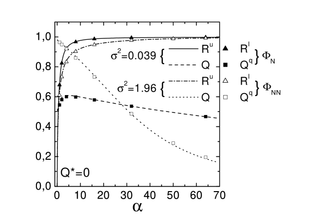
Figure 1: Order parameters of SVMs for purely linear teacher rules, $Q_{*}=0$. Symbols are experimental results for input space dimension $n=50$, corresponding to the two kinds of quadratic mappings, $\Phi_{N}$ with $a=1/\sqrt{n}$ (full symbols) and $\Phi_{NN}$ with normalizing factor $a=1$ (open symbols) respectively. Error bars are smaller than the symbols. The lines are not fits, but the solutions of the Statistical Mechanics equations for $\Delta=(n+1)/2$ and $\sigma^{2}=na^{2}/\Delta$ with $n=50$, and $a$ corresponding to each mapping.

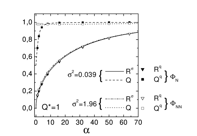
Figure 2: Order parameters of SVMs for purely quadratic teacher rules, $Q_{*}=1$. Definitions are the same as in figure 1.

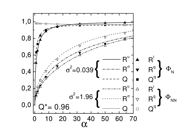
Figure 3: Order parameters of SVMs for isotropic teacher rules, $Q_{*;\,iso}=\Delta/(1+\Delta)$. Definitions are the same as in figure 1.

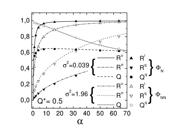
Figure 4: Order parameters of SVMs for a general teacher rule, $Q_{*}=0.5$. Definitions are the same as in figure 1.

Fig. 1 corresponds to a purely linear teacher ($Q_{*}=0$), i.e. to a quadratic SVM learning a rule linearly separable in input space. As in this case $R^{\sigma}=0$ because ${\bf w}_{*}^{\sigma}=0$, only $R^{u}$ and $Q$ are represented. Conversely, in the case of a purely quadratic rule, $Q_{*}=1$, represented on fig. 2, $R^{u}=0$. Notice that $Q\rightarrow Q_{*}$ for $\alpha\rightarrow\infty$ in both cases, meaning that the student learns in which subspace lies the teacher. Correspondingly, the normalized teacher-student overlap increases smoothly to $1$. However, the pace at which these quantities reach their asymptotic limit depends on the features normalization factor, and it is their combination given by eq. (19) that determines the generalization error $\epsilon_{g}$, represented on fig. 5. Clearly, if $Q_{*}=0$, i.e. if the problem is linearly separable in input space, the normalized mapping has lower $\epsilon_{g}$ at finite $\alpha$. Conversely, if the discriminating surface is purely quadratic in input space, the non-normalized mapping gives better results. In the asymptotic limit $\alpha\rightarrow\infty$ the mapping’s normalization becomes irrelevant, as in both cases the generalization error vanishes.

Fig. 3 shows the results corresponding to the isotropic teacher, $Q_{*}=Q_{*;\,iso}\equiv\Delta/(1+\Delta)$. For $\Delta=25.5$ we have $Q_{*;\,iso}=0.962$. A particular case of such a teacher, considered in [Dietrich et al. (1999), Yoon and Oh (1998)], has all its weight components of equal absolute value $|w_{*,\nu}|=|w_{*,\nu\mu}|=1$. Finally, the results corresponding to a general rule, with $Q_{*}=0.5$, are shown in fig. 4.

Notice that, irrespective of the mapping, the overlaps $R^{u}$ and $R^{\sigma}$ present different behaviours, as the latter increases much slower than the former. This reflects the fact that, as the number of quadratic components scales like $n\Delta$, a number of examples of the order of $n\Delta$ are needed to learn them. Thus, as a function of $\alpha$, the linear components are learned first. Indeed, $R^{u}$ reaches a value close to $1$ with $\alpha\sim O(1)$ while $R^{\sigma}$ needs $\alpha\sim O(\Delta)$ to reach similar values. We call this general trend hierarchical learning.

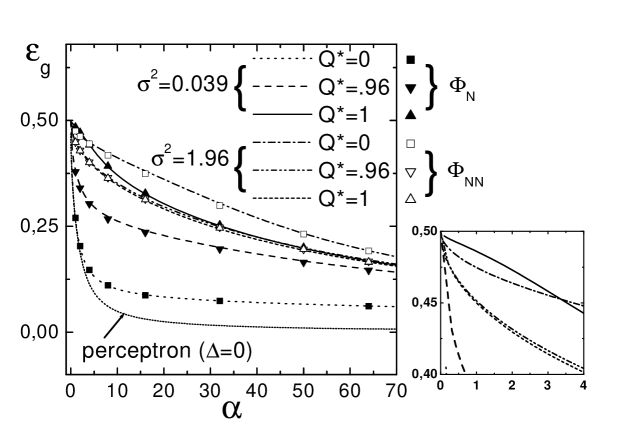
Figure 5: Learning curves of SVMs for different teacher rules $Q_{*}$. Definitions are the same as in figure 1. The inset is an enlargement of the small $\alpha$ region.

As the generalization error depends on $R^{u}$ and $R^{\sigma}$ through the combination (19), the signature of hierarchical learning is present on the learning curves $\epsilon_{g}$ corresponding to the different rules, plotted against $\alpha$ on fig. 5. The performance obtained with the normalized mapping is better the smaller the value of $Q_{*}$. The non-normalized mapping shows the opposite trend: its performance for a purely linear teacher ($Q_{*}=0$) is extremely bad, but it improves for increasing values of $Q_{*}$ and slightly overrides that of the normalized mapping in the case of a purely quadratic teacher.

These results reflect the competition on learning the anisotropically distributed features. The more the features are compressed, the more difficult the learning task. In the case of rules with $Q_{*}\ll 1$, the linear components carry the most significant information. In those cases, it is advantageous to use the normalized mapping, which has the $\sigma$-components compressed ($\sigma^{2}=0.039$) with respect to the u-components, which have unit variance.

The non-normalized mapping has $\sigma^{2}=1.96$, meaning that the compressed components are those of the u-subspace. This mapping is better whenever most of the information is contained in the $\sigma$-subspace, which is the case for teachers with large $Q_{*}$ and, in particular, with $Q_{*}=1$. In this last case, the linear components only introduce noise that hinders the learning process. As the number of linear components is much smaller than the number of quadratic ones, their pernicious effect is expected to be more conspicuous the smaller the value of $\Delta$.

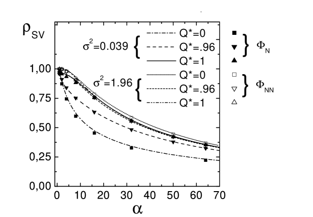
Figure 6: Fraction of learning patterns that belong to the subset of Support Vectors.

Finally, for the sake of completeness, the fraction of support vectors $\rho_{SV}\equiv\ell_{SV}/\ell$, where $\ell_{SV}$ is the number of training patterns with maximal stability, is represented on figure 6. Notice that, although these curves present qualitatively the same trends as $\epsilon_{g}$, they constitute a very loose bound to the latter. Since the student’s weights can be expressed as a linear combination of SVs [Vapnik (1995)], this result is of practical interest. It shows that increasing the number of training patterns does not increase the typical number of non-vanishing coefficients that have to be determined using the quadratic minimization program: although at low $\alpha$ most of the training patterns are expected to be support vectors, this fraction decreases smoothly with $\alpha$. Notice that $\alpha$ in our approach is the number of training patterns per input space dimension. Thus, even if $\rho_{SV}$ may seem large, this is not so in regard to the dimension of the feature space. In our simulations for example, $\alpha=50$ is of the order of the VC-dimension of the feature space. However, from fig. 6 we expect that less than half of the training patterns be SVs.

5 Discussion

In order to understand the results obtained in the previous section, we first consider the relative behaviour of $R^{u}$ and $R^{\sigma}$, deduced from the theoretical approach. If $\Delta_{*}^{\sigma}\ll\Delta$, which is the case for sufficiently small $Q_{*}$, we get that $R^{\sigma}\ll R^{u}$. This means that the quadratic components are more difficult to learn than the linear ones. On the other hand, if the teacher lies mainly in the quadratic subspace, $\Delta_{*}^{\sigma}\gg\Delta$ and $R^{\sigma}>R^{u}$. The crossover between these different behaviours occurs at $\Delta_{*}^{\sigma}=\Delta$, for which $R^{\sigma}=R^{u}$. For $n=50$, this arises for $Q_{*}=0.998$ for the normalized mapping and for $Q_{*}=0.929$ for the non-normalized one. In the particular case of the isotropic teacher and the non-normalized mapping, $Q_{*;\,iso}>0.929$, so that $R^{\sigma}>R^{u}$, as shown on figure 3.

These considerations alone are not sufficient to understand the behaviour of the generalization error, which depends on the weighted sum of $R^{\sigma}$ and $R^{u}$ (see equation (19)). The behaviour of $R^{\sigma}$ and $R^{u}$ at small $\alpha$ is useful to understand the onset of hierarchical learning. In the limit $\alpha\rightarrow 0$, we find that $Q\simeq\Delta\sigma^{2}/(\Delta\sigma^{2}+1)$ to leading order in $\alpha$. This result may be understood with the following simple argument: if there is only one training pattern, clearly it is a SV and the student’s weight vector is proportional to it. As a typical example has $n$ components of unit length in the u-subspace and $n\Delta$ components of length $\sigma$ in the $\sigma$-subspace, we have $Q=n\Delta\sigma^{2}/(n\Delta\sigma^{2}+n)$. With the normalized mapping, $\lim_{\alpha\rightarrow 0}Q=1/2$. In the case of the non normalized one $\lim_{\alpha\rightarrow 0}Q=(2\Delta-1)/2\Delta$, which depends on the inflation factor of the SVM. In this limit, we obtain:

$$\kappa \simeq \frac{1+\sigma^{2}\Delta}{\sqrt{1+\sigma^{4}\Delta}}\frac{1}{\sqrt{\alpha}},$$ (22)

$$R^{u} \simeq \sqrt{\frac{2}{\pi}}\frac{1}{\sqrt{1+\Delta_{*}^{\sigma}}}\sqrt{\alpha},$$ (23)

$$R^{\sigma} \simeq \sqrt{\frac{2}{\pi}}\,\sqrt{\frac{\Delta_{*}^{\sigma}}{1+\Delta_{*}^{\sigma}}}\,\sqrt{\frac{\alpha}{\Delta}}.$$ (24)

Therefore, $R\sim\sqrt{\alpha}$ for $\alpha\ll 1$, as for the simple perceptron MMH [Gordon and Grempel (1995)], but with a prefactor that depends on the mapping and the teacher.

In our model, we expect that hierarchical learning correspond to a fast increase of $R$ at small $\alpha$, mainly dominated by the contribution of $R^{u}$. As in the limit $\alpha\rightarrow 0$,

$$R\simeq\frac{R^{u}+R^{\sigma}\sqrt{\sigma^{4}\Delta\Delta_{*}^{\sigma}}}{\sqrt{1+\sigma^{4}\Delta}\sqrt{1+\Delta_{*}^{\sigma}}},$$ (25)

we do not expect to have hierarchical learning if $\sigma^{4}\Delta\gg 1$, as in that case mainly $R^{\sigma}$ contributes to $R$. This is what happens with the non normalized mapping. On the other hand, hierarchical learning takes place if $\sigma^{4}\Delta\ll 1$ and $\Delta_{*}^{\sigma}\lesssim 1$. The first condition establishes a constraint on the mapping, which is only satisfied by the normalized one. The second condition, that ensures that $R^{\sigma}<R^{u}$ holds, gives the range of teachers for which this hierarchical generalization takes place. Under these conditions, $R$ grows fast and the contribution of $R^{\sigma}$ is negligible because it is weighted by $\sqrt{\sigma^{4}\Delta\Delta_{*}^{\sigma}}$. The effect of hierarchical learning is more important the smaller $\Delta_{*}^{\sigma}$. The most dramatic effect arises for $Q_{*}=0$, i.e. for a quadratic SVM learning a linearly separable rule.

Notice that if the normalized mapping is used, the condition $\Delta_{*}^{\sigma}\lesssim 1$ implies that $Q_{*}<Q_{*;\,iso}\equiv\Delta/(1+\Delta)$, where $Q_{*;\,iso}$ corresponds to the isotropic teacher. A straightforward calculation shows that if the teachers are drawn at random on the surface of the hypersphere in feature space, the distribution of $Q_{*}$ is highly non symmetric, with a maximum at the value of $Q_{*;\,iso}$, that depends on $n$. The fraction of teachers with $Q_{*}<Q_{*;\,iso}$ is smaller than $1/2$. For example, only $47.5\%$ of the teachers satisfy this constraint if $n=50$. When $n\rightarrow\infty$, the distribution becomes $\delta(Q_{*}-Q_{*;\,iso})$, and $Q_{*;\,iso}$ tends to the median, meaning that in this limit, only about $50\%$ of the teachers give rise to hierarchical learning when using the normalized mapping.

In the limit $\alpha\rightarrow\infty$, all the generalization error curves converge to the same asymptotic value as the simple perceptron MMH learning in the feature space, namely $\epsilon_{g}=0.500489(1+\Delta)/\alpha$, independently of $\sigma$ and $Q_{*}$. Thus, $\epsilon_{g}$ vanishes slower the larger the inflation factor $\Delta$.

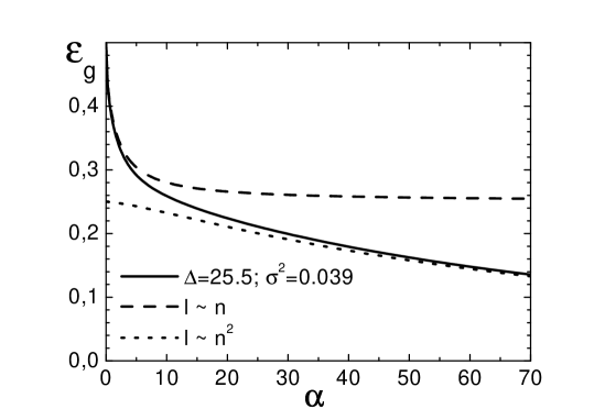
Figure 7: Generalization error of a SVM corresponding to different thermodynamic limits. See the text for the definition of $\alpha$ in each regime.

Since the inflation factor $\Delta$ of the SVM feature space in our approach is a free parameter, it does not diverge in the thermodynamic limit $N\rightarrow\infty$ . As a consequence, the two scaling regimes for $\epsilon_{g}$ give rise to a simple crossover between a fast decrease at small $\alpha$ followed by a slow decrease at large $\alpha$. The results of Dietrich et al. [Dietrich et al. (1999)] for the normalized mapping, that corresponds to $\sigma^{2}\Delta=1$ in our model, can be deduced by taking appropriately the limits before solving our saddle point equations. The regime where the number of training patterns $\ell=\alpha n$ scales with $n$, is straightforward. It is obtained, within our approach, by taking the limit $\sigma\rightarrow 0$ and $\Delta\rightarrow\infty$ keeping $\sigma^{2}\Delta=1$ and $\alpha$ finite. The regime where the number of training patterns $\ell=\alpha n$ scales with $n\Delta$, the number of quadratic features, is obtained by keeping $\tilde{\alpha}\equiv\alpha/(1+\Delta)$ finite whilst taking, here again, the limit $\sigma\rightarrow 0$, $\Delta\rightarrow\infty$ with $\sigma^{2}\Delta=1$. The corresponding curves are represented on figure 7 for the case of an isotropic teacher. In order to compare with our results at finite $\Delta$, the regime where $\tilde{\alpha}$ is finite is represented as a function of $\alpha=(1+\Delta)\tilde{\alpha}$ using the value of $\Delta$ corresponding to $n=50$, namely, $\Delta=25.5$. In the same figure we represented the generalization error $\epsilon_{g}$ obtained with our model using the parameter values $\sigma^{2}=0.039$ and $\Delta=25.5$.

These results, obtained for quadratic SVMs, are easily generalizable to higher order polynomial SVMs, as is the case with the approach of [Dietrich et al. (1999)]. We expect a cascade of hierarchical decreasings of the generalization error as a function of $\alpha$, in which successively more and more compressed features are learned.

6 Conclusion

We introduced a model that clarifies some aspects of the generalization properties of polynomial Support Vector Machines (SVMs) in high dimensional feature spaces. To this end, we focused on quadratic SVMs. The quadratic features, which are the pairwise products of input components, may be scaled by a normalizing factor. Depending on its value, the generalization error presents very different behaviours in the thermodynamic limit [Dietrich et al. (1999), Buhot and Gordon (1999)].

We showed that any finite size quadratic SVM may be characterized by two parameters: $\Delta$ and $\sigma$. The inflation factor $\Delta$ is the number of quadratic features relative to the number of input features, and is proportional to the input space dimension $n$. The variance $\sigma$ of the quadratic features is related to the normalizing factor. Usually, either $\sigma\sim 1/\sqrt{n}$ (normalized mapping) or $\sigma\sim 1$ (non normalized mapping). In previous studies, not only the input space dimension diverges in the thermodynamic limit $n\rightarrow\infty$, but also $\Delta$ and $\sigma$ are correspondingly scaled.

In our model, the proportion of quadratic features $\Delta$ and their variance $\sigma$ are considered as parameters characterizing the (finite size) SVMs. Since we keep them constant when taking the thermodynamic limit, we can study the learning properties of actual SVMs with finite inflation ratios and normalizing factors, as a function of $\alpha\equiv\ell/n$, where $\ell$ is the number of training examples.

Our theoretical results were obtained neglecting the correlations among the quadratic features. Indeed, their effect does not seem to be important, as the agreement between our computer experiments with actual SVMs and the theoretical predictions is excellent. This approximation was also shown to give good predictions in other similar problems [Dietrich et al. (1999), Yoon and Oh (1998)], but further investigations are needed to establish rigorously the conditions of its validity.

We find that the generalization error $\epsilon_{g}$ depends on the type of rule to be inferred through $Q_{*}$, the (normalized) teacher’s squared weight components in the quadratic subspace. If the normalized mapping is used and $Q_{*}$ is small enough, the behaviour of $\epsilon_{g}$ at small $\alpha$ is dominated by the high rate learning of the linear components. On increasing $\alpha$, there is a crossover to a regime where the decrease of $\epsilon_{g}$ becomes much slower. This crossover becomes smoother for increasing values of $Q_{*}$, and this effect of hierarchical learning disappears for large enough $Q_{*}$. If the limits $\Delta\sim n\rightarrow\infty$ and $\sigma^{2}\sim 1/n\rightarrow 0$ are taken together with the thermodynamic limit, the hierarchical learning effect gives rise to the different scaling regimes, corresponding to $\ell\sim n$ or $\ell\sim n^{2}$, described previously [Yoon and Oh (1998), Dietrich et al. (1999)].

On the other hand, if the features are not normalized, the contributions of both the linear and the quadratic components to $\epsilon_{g}$ are of the same order, and there is no hierarchical learning at all. For $Q_{*}>Q_{*;\,iso}$, which corresponds to the isotropic teacher, the non normalized mapping has a slightly smaller generalization error than the normalized one.

It is worth remarking that if the rule to be learned allows for hierarchical learning, the generalization error of the normalized mapping is much smaller than that of the non normalized one. In fact, the teachers corresponding to such rules are those with $Q_{*}\lesssim Q_{*;iso}$, where $Q_{*;\,iso}$ corresponds to the isotropic teacher, the one having all its weights components equal. For the others, both the normalized mapping and the non normalized one present similar performances. If the weights of the teacher are selected at random on a hypersphere in feature space, the most probable teachers have precisely $Q_{*}=Q_{*;\,iso}$, and the fraction of teachers with $Q_{*}\leq Q_{*;\,iso}$ represent of the order of $50\%$ of the inferable rules. Thus, from a practical point of view, without having any prior knowledge about the rule underlying a set of examples, the normalized mapping should be preferred.

Appendix

The average (11) within the replica approach can be expressed as a function of several order parameters, whose values have to minimize the free energy of the system. Among these, the overlaps of the weights corresponding to different replicas, $a,b$,

$$q^{u}_{ab} = \sum_{\nu=1}^{n}\overline{\langle w_{a;\nu}w_{b;\nu}\rangle}/\tilde{n},$$

$$q^{\sigma}_{ab} = \sum_{\nu=n+1}^{\tilde{n}}\overline{\langle w_{a;\nu}w_{b;\nu}\rangle}/\tilde{n}.$$ (26)

As the tasks considered are learnable, the solution that minimizes the cost function (12) with maximal $\kappa$ is unique. Thus, in the following we may assume that replica symmetry holds. Then, $q_{u}^{ab}=q_{u}$, $q_{\sigma}^{ab}=q_{\sigma}$ for all $a,b$, and the saddle point equations corresponding to the extremum of the free energy for the MMH are:

$$2\frac{\alpha}{\Delta}\Delta^{\sigma}I_{1} = (1-(R^{\sigma})^{2})\,\frac{(x+\Delta^{\sigma})^{2}}{1+\Delta^{\sigma}},$$ (27)

$$2\frac{\alpha}{\Delta}I_{2} = \sqrt{\frac{1+\Delta_{*}^{\sigma}}{\Delta_{*}^{\sigma}}}\,R^{\sigma}\,\frac{x+\Delta^{\sigma}}{\sqrt{\Delta^{\sigma}(1+\Delta^{\sigma})}},$$ (28)

$$2\frac{\alpha}{\Delta}Q(1-\sigma^{2})I_{3} = \left(1-x\frac{1-(R^{\sigma})^{2}}{1-(R^{u})^{2}}\right)\,\frac{x+\Delta^{\sigma}}{1+\Delta^{\sigma}},$$ (29)

$$\frac{(R^{\sigma})^{2}}{1-(R^{\sigma})^{2}} = \frac{\Delta_{*}^{\sigma}}{\Delta}\frac{(R^{u})^{2}}{1-(R^{u})^{2}},$$ (30)

$$\frac{R^{u}}{R^{\sigma}} = x\frac{\Delta}{\sqrt{\Delta^{\sigma}\Delta_{*}^{\sigma}}}.$$ (31)

where $\Delta^{\sigma}$ and $\Delta_{*}^{\sigma}$ are defined by eq. (20), $Q_{*}$, $Q$, $R^{u}$ and $R^{\sigma}$ by equations (13) to (16), and $x\equiv lim_{\kappa\rightarrow\kappa_{max}}(1-q_{u}/(1-Q))/(1-q_{\sigma}/Q)$. The integrals in the left hand side of equations (27-29) are

$$I_{1} = \int_{-\tilde{\kappa}}^{\infty}Dt\,(t+{\tilde{\kappa}})^{2}\,H\left(\frac{tR}{\sqrt{1-R^{2}}}\right),$$ (32)

$$I_{2} = \frac{1}{\sqrt{2\pi}}\left[\frac{\sqrt{1-R^{2}}\exp(-{\tilde{\kappa}^{2}}/(2(1-R^{2})))}{\sqrt{2\pi}}+{\tilde{\kappa}}H\left(\frac{-\tilde{\kappa}}{\sqrt{1-R^{2}}}\right)\right],$$ (33)

$$I_{3} = \int_{-\tilde{\kappa}}^{\infty}Dt\,\tilde{\kappa}\,(t+{\tilde{\kappa}})\,H\left(\frac{tR}{\sqrt{1-R^{2}}}\right),$$ (34)

with $Dt\equiv dt\,\exp{(-t^{2}/2)}/\sqrt{2\pi}$, $H(x)=\int_{x}^{\infty}Dt$, $R$ is given in eq. (19), and

$$\tilde{\kappa}=\frac{\kappa_{max}}{\sqrt{(1-Q)(1+\Delta^{\sigma})}}.$$ (35)

After solving the above equations for $Q$, $R^{u}$, $R^{\sigma}$, $x$ and $\tilde{\kappa}$, they allow to determine $\rho_{SV}$ and $\epsilon_{g}$ through (21) and (18).

References

- Buhot et al. (1997) A. Buhot, J-M. Torres Moreno and M. B. Gordon. Finite size scaling of the bayesian perceptron Phys.Rev.E, 55:7434–7440, 1997.
- Buhot and Gordon (1999) A. Buhot and M. B. Gordon. Learning properties of Support Vector Machines In Michel Verleysen, editor, Proceedings of ESANN’99-European Symposium on Artificial Neural Networks, 1998.
- Cortes and Vapnik (1995) C. Cortes and V. Vapnik. Support Vector Networks Machine Learning, 20:273–297, 1995.
- Dietrich et al. (1999) R. Dietrich, M. Opper, and H. Sompolinsky. Statistical mechanics of Support Vector Networks Phys. Rev. Lett, 82:2975–2978, 1999.
- Gardner and Derrida (1988) E. Gardner and B. Derrida. Optimal storage properties of neural networks models J. Phys A, 21:271–284, 1988.
- Gordon and Grempel (1995) M. B. Gordon and D. R. Grempel. Learning with a temperature-dependent algorithm Europhys. Lett., 29:257–262, 1995.
- Marangi et al. (1995) C. Marangi, M. Biehl and S. Solla. Supervised learning from clustered input examples Europhys. Lett, 30:117–122, 1995.
- Mézard et al. (1987) M. Mézard, G. Parisi and M. A. Virasoro Spin glasses and beyond. World Scientific, Singapore, 1987.
- Monasson (1993) R. Monasson. Storage of spatially correlated patterns in autoassociative memories J. Phys. A, 25:1141–1152, 1993.
- Nadler and Fink (1997) W. Nadler and W. Fink. Finite size scaling in neural networks Phys. Rev. Lett., 78:555–558, 1997.
- Opper et al. (1990) M. Opper, W. Kinzel, J. Kleinz and R. Nehl. On the Ability of the Optimal Perceptron to Generalise J. Phys. A: Math. Gen. 23: L-581–L586, 1990.
- Opper and Kinzel (1995) M. Opper and W. Kinzel. Statistical mechanics of generalization In E. Domany, J.L. van Hemmen, editors, Models of Neural Networks III. Springer-Verlag, Physics of Neural Networks Series, Berlin, 1995.
- Risau-Gusman and Gordon (2000) S. Risau-Gusman and M. B. Gordon. Understanding stepwise generalization of Support vector Machines : a toy model in Advances in Neural Information Processing Systems 12, S. A. Solla, T. K. Leen and K.-R. M ller(eds.), MIT Press, 321–327, 2000.
- Schroder and Urbanczik (1998) M. Schroder and R. Urbanczik. Comment on “Finite Size Scaling in Neural Networks” Phys. Rev. Lett., 80:4109, 1998.
- Seung et al. (1992) H.S. Seung, H. S. Sompolinsky and N. Tishby. Statistical mechanics of learning from examples Phys. Rev. A, 45:6056–6090, 1992.
- Smola (1999) A. Smola. Program available upon request to http://svm.first.gmd.de.
- Talagrand (1998) M. Talagrand. Self averaging and the space of interactions in neural networks Random Structures and Algorithms, 14:199–213. 1998.
- Vanderbei (1998) R. J. Vanderbei. Loqo, an interior point code for quadratic programming Technical Report SOR-94-15, Princeton University.
- Vapnik (1995) V. Vapnik. The nature of statistical learning theory. Springer Verlag, New York, 1995.
- Vapnik and Chapelle (2000) V. Vapnik and O. Chapelle. Bounds on error expectation for Support Vector Machines Neural Computation, 12:2013–2036. 2000.
- Watkin et al. (1993) T. L. H. Watkin, A. Rau and M. Biehl. The statistical mechanics of learning a rule Rev. Mod. Phys., 65:499–555, 1993.
- Yoon and Oh (1998) H. Yoon and J.-H. Oh. Learning of higher order perceptrons with tunable complexities J. Phys. A: Math. Gen., 31:7771–7784, 1998.