Non-perturbative effective field theory for two-leg antiferromagnetic spin ladders

Abstract

We study the long wavelength limit of a spin $1/2$ Heisenberg antiferromagnetic two-leg ladder, treating the interchain coupling in a non-perturbative way. We perform a mean field analysis and then include exactly the fluctuations. This allows for a discussion of the phase diagram of the system and provides an effective field theory for the low energy excitations. The coset fermionic Lagrangian obtained corresponds to a perturbed $SU(4)_{1}/U(1)$ Conformal Field Theory (CFT). This effective theory is naturally embedded in a $SU(2)_{2}\times Z_{2}$ CFT, where perturbations are easily identified in terms of conformal operators in the two sectors. Crossed and zig-zag ladders are also discussed using the same approach.

I Introduction

Antiferromagnetic Heisenberg spin ladders have been a subject of central interest during the last years. These are intermediate systems between the gapless critical spin $1/2$ Heisenberg chain and the ordered spin $1/2$ 2D system relevant for undoped cuprate superconductors. The simplest realization, i.e. the two-leg ladder, shows a dramatic different excitation spectrum with respect to the one of an isolated chain. It has a finite gap to the first excitation and magnetic correlations are short ranged. Several inorganic compounds have been recently synthesized and modeled as Heisenberg ladders [1]. Exponential decay of the low temperature magnetic susceptibility was the first signal of the existence of a spin gap in two-leg ladder materials. Neutron and optical measurements also manifest the presence of a gap and are consistently described by a two-leg ladder model with exchange integrals of the same order in the chains direction($J$) and along the rungs ($J^{\prime}$).

Theoretically, the existence of a gap was early predicted from numerical exact diagonalization and strong coupling perturbation theory ($J/J^{\prime}\ll 1$) [2]. More recently field theoretical technics have been used to analyze the excitation spectrum in the weak coupling regime ($J^{\prime}/J\ll 1$) [3, 4]. These treatments give access to the whole low energy excitation spectrum as well as to the dynamical susceptibilities, which are essential to compare with experimental probes. The philosophy underlying this study is the following: spin operators are expressed in the well known bosonized representation of each chain and the interchain coupling is treated as a small perturbation in this representation. The applicability of these studies is then valid in principle only in the weak coupling regime and its use in the description of e.g. the experimentally realized two-leg ladders in which $J^{\prime}\sim J/2$ should be taken with some care. It is therefore not clear up to which value of $\frac{J^{\prime}}{J}$ the results of [3, 4] are applicable, and it is important to develop theoretical methods which could be used beyond the weak coupling regime.

The picture that emerges from the weak coupling analysis leads to a description in terms of triplet of massive Majorana fermions and a singlet Majorana fermion with a different mass (which has been estimated to be minus three times the triplet mass) [4]. The only interactions between these fermions are marginal current-current terms which have been argued to simply renormalize their masses and velocities. A question, that has been risen in recent studies of the Raman scattering spectrum [5], is whether marginal interactions can in fact be disregarded. In particular, correlation functions obtained disregarding marginal interactions apparently do not fit experiments (see e.g. [6]).

In this work we analyze the complete phase diagram of the two-leg antiferromagnetic ladder. Our approach, first used here for spin ladders, starts from a fermionic representation of the spin operators in the functional integral framework, as introduced in [7, 8, 9] for spin chains. With a simple Ansatz to the Mean Field (MF) configurations we show that the system undergoes a cross-over from a weak to a strong coupling regime at an intermediate value of $J^{\prime}/J$. We then introduce fluctuations around MF and take them into account to all orders to construct the low energy effective field theory.

The resulting theory corresponds to a coset Conformal Field Theory (CFT) of symmetry $SU(4)_{1}/U(1)_{iso}$, perturbed by relevant operators (of dimension $1$) and marginal operators (of dimension $2$) arising from the single occupancy constraint as well as from the amplitude fluctuations of the link fields introduced to decouple the fermionic interactions. It should be noted that our approach is based on the assumption that the local single occupancy constraint can be implemented as a very last step, while it is taken into account globally from the beginning. The correctness of this procedure is not guaranteed from first principles, but is supported a posteriori.

We show that the complete structure of these perturbations can be retained and that they take a simple form in the language of conformal embeddings. In particular, the marginal terms which arise can be easily classified in the new language and their effect can then be studied in a non-perturbative way. When the relevant perturbations are expressed in the embedded $SU(2)_{2}\times Z_{2}$ CFT language the spectrum is naturally separated in the triplet and singlet of Majorana fermions. These results, which are valid up to $J^{\prime}/J\approx 8/\pi^{2}$, extend to finite coupling the weak coupling study of [4]. It should be stressed that recent estimates of the ratio of exchange constants lead to values of $J^{\prime}/J$ around $1/2$ in several cuprate materials [10].

In order to illustrate the generality and ease of use of our approach, it is then applied to the so-called crossed ladders and zig-zag ladders. Phase diagrams and low energy theories are obtained in the region containing the weak coupling limit; further analysis and details will be considered elsewhere.

The paper is organized as follows. In Section II we introduce the model, present Hubbard-Stratonovich decoupling technics and perform a MF analysis, discussing the resulting phase diagram. In Section III we construct the low energy effective field theory: our theory contains four Dirac fermionic species corresponding to the spin and band indices of the ladder. In Section IV we show that the theory has a natural relation to $SU(2)_{2}\times Z_{2}$ CFT through conformal embedding (the last part arises from the two electronic bands). In Section V we briefly report results on crossed and zig-zag ladders. Finally, in Section VI the conclusions and possible further developments of our method are given.

II Mean field analysis

We consider the Heisenberg Hamiltonian for a two-leg spin $1/2$ ladder,

$$H=\sum_{n=1}^{N}\sum_{l=1}^{2}\left(J{\vec{S}}^{(l)}_{n}.{\vec{S}}^{(l)}_{n+1}+\frac{J^{\prime}}{2}{\vec{S}}^{(l)}_{n}.{\vec{S}}^{(l+1)}_{n}\right)$$ (1)

where $N$ is the number of sites along the chains, $J>0$ and $J^{\prime}>0$ are the couplings between adjacent spins along the legs and rungs respectively. For mathematical convenience we assume periodic boundary conditions (P.B.C.) in both directions (notice that the Hamiltonian is suitable written for arbitrary $n$-leg ladders; in the present case the physical coupling along the rungs is in effect $J^{\prime}$).

The spin variables can be represented in terms of fermionic operators with spin $c^{(l)}_{n,\alpha}$ as

$${\vec{S}}^{(l)}_{n}=c^{\dagger(l)}_{n,\alpha}\frac{{\vec{\sigma}}_{\alpha\beta}}{2}c^{(l)}_{n,\beta},$$ (2)

where $\vec{\sigma}$ are Pauli matrices, together with a local constraint that ensures one spin per site, imposed on the physical states by

$$c^{\dagger(l)}_{n,\alpha}c^{(l)}_{n,\alpha}|phys\rangle=|phys\rangle\ .$$ (3)

Throughout this paper we will not use the summation convention neither for site nor leg indices; repeated spin (Greek) indices are summed.

Using (2) and (3) the Hamiltonian (1) can be rewritten as

$$H=-\sum_{n=1}^{N}\sum_{l=1}^{2}\left(\frac{J}{2}c^{\dagger(l)}_{n,\alpha}c^{(l)}_{n+1,\alpha}c^{\dagger(l)}_{n+1,\beta}c^{(l)}_{n,\beta}+\frac{J^{\prime}}{4}c^{\dagger(l)}_{n,\alpha}c^{(l+1)}_{n,\alpha}c^{\dagger(l+1)}_{n,\beta}c^{(l)}_{n,\beta}\right)+C$$ (4)

where $C=-N/2$ is an irrelevant constant term.

We now trade (4) for a quadratic Hamiltonian via a Hubbard-Stratonovich transformation, at the usual price of introducing auxiliary fields $B^{(l)}_{n}$ associated to terms containing $c^{\dagger(l)}_{n+1,\alpha}c^{(l)}_{n,\alpha}$ and $B^{\prime}_{n}$ associated to terms containing $c^{\dagger(l+1)}_{n,\beta}c^{(l)}_{n,\beta}$. It is natural to interpret $B^{(l)}_{n}$ as localized on the leg $(l)$ links between sites $n$ and $n+1$ and $B^{\prime}_{n}$ as localized on the rung links. After the transformation the Hamiltonian reads

$$H = \frac{J}{2}\sum_{n=1}^{N}\sum_{l=1}^{2}\left(B^{(l)}_{n}c^{\dagger(l)}_{n,\alpha}c^{(l)}_{n+1,\alpha}+B^{\dagger(l)}_{n}c^{\dagger(l)}_{n+1,\beta}c^{(l)}_{n,\beta}+B^{\dagger(l)}_{n}B^{(l)}_{n}\right)$$ (5)

$$+ \frac{J^{\prime}}{4}\sum_{n=1}^{N}\sum_{l=1}^{2}\left(B^{\prime}_{n}c^{\dagger(l)}_{n,\alpha}c^{(l+1)}_{n,\alpha}+B^{\dagger^{\prime}}_{n}c^{\dagger(l+1)}_{n,\beta}c^{(l)}_{n,\beta}+B^{\dagger^{\prime}}_{n}B^{{}^{\prime}}_{n}\right)$$ (6)

As we look for a low energy effective theory, we treat the $B$ variables in a long wave approximation. To this end, we parameterize these fields in terms of real MF values $(B_{0},B^{{}^{\prime}}_{0})$ and fluctuations

$$B^{(l)}_{n}=B_{0}\exp(iaA^{(l)}_{n}+aR^{(l)}_{n}),\ \ \ B^{{}^{\prime}}_{n}=B^{{}^{\prime}}_{0}\exp(iaA^{{}^{\prime}}_{n}+aR^{{}^{\prime}}_{n})\ .$$ (7)

Notice that we have included both phase and amplitude fluctuations, which will play important different rôles in the following. For this reason, we explicitly distinguish the Hermitean $(R^{(l)}_{n},R^{{}^{\prime}(l)}_{n})$, and anti-Hermitean $(iA^{(l)}_{n},iA^{{}^{\prime}(l)}_{n})$ parts of the fluctuation fields. The expression for $B^{{}^{\prime}}_{n}$ will be eventually modified when $B^{{}^{\prime}}_{0}=0$ (see eq. (37)).

As a first step, we perform the MF evaluation of the Hamiltonian (6) by setting the fluctuations to zero. The resulting MF Hamiltonian is then a tight-binding model for two coupled chains,

$$H_{mf} = -t\sum_{n=1}^{N}\sum_{l=1}^{2}\left(c^{\dagger(l)}_{n,\alpha}c^{(l)}_{n+1,\alpha}+c^{\dagger(l)}_{n+1,\beta}c^{(l)}_{n,\beta}\right)-2t^{\prime}\sum_{n=1}^{N}\left(c^{\dagger(1)}_{n,\alpha}c^{(2)}_{n,\alpha}+c^{\dagger(2)}_{n,\beta}c^{(1)}_{n,\beta}\right)$$ (9)

$$+\frac{4N}{J}t^{2}+\frac{8N}{J^{\prime}}{t^{\prime}}^{2},$$

where

$$t=-\frac{JB_{0}}{2},\ \ \ t^{\prime}=-\frac{J^{\prime}B^{{}^{\prime}}_{0}}{4}\ .$$ (10)

The coupled tight-binding model is easily diagonalized by means of a double Fourier transform. We first decouple two bands by means of

$$c^{(1)}_{n,\alpha}=\frac{1}{\sqrt{2}}(c^{(+)}_{n,\alpha}-c^{(-)}_{n,\alpha}),$$ (11)

$$c^{(2)}_{n,\alpha}=\frac{1}{\sqrt{2}}(c^{(+)}_{n,\alpha}+c^{(-)}_{n,\alpha})$$ (12)

and then introduce pseudo-momentum operators $d^{(+)},d^{(-)}$ by

$$c^{(+)}_{n,\alpha}=\frac{1}{\sqrt{2N}}\sum_{m=1}^{N}d^{(+)}_{m,\alpha}\exp(-i\frac{2\pi mn}{N}),$$ (13)

$$c^{(-)}_{n,\alpha}=\frac{1}{\sqrt{2N}}\sum_{m=1}^{N}d^{(-)}_{m,\alpha}\exp(-i\frac{2\pi mn}{N}),$$ (14)

in terms of which the Hamiltonian reads

$$H_{mf} = -\sum_{m=1}^{N}(2t\cos(\frac{2\pi}{N}m)+2t^{\prime})d^{\dagger(+)}_{m,\alpha}d^{(+)}_{m,\alpha}-$$ (16)

$$\sum_{m=1}^{N}(2t\cos(\frac{2\pi}{N}m)-2t^{\prime})d^{\dagger(-)}_{m,\alpha}d^{(-)}_{m,\alpha}+\frac{4N}{J}t^{2}+\frac{8N}{J^{\prime}}{t^{\prime}}^{2}.$$

This expression clearly represents a decoupled two-band tight-binding model.

The constraint (3), meaning one electron per site, forces the system to be exactly at half filling. Low-energy excitations are then achieved by creating holes just below the Fermi surface and creating electrons just above it[11]. Notice that this can be done only if

$$|t^{\prime}|<|t|,$$ (17)

that is when the Fermi level crosses both bands. If this condition is not satisfied, the system presents a finite energy gap to spin excitations.

The actual values of $t$ and $t^{\prime}$ are determined by minimizing the energy of (16). In order to perform this evaluation we introduce a lattice spacing $a$ and a position coordinate $x=na$ ($x\in[0,L=Na]$); the appropriate pseudo-momentum coordinate is $k=m2\pi/(Na)$ ($k\in[-\pi/a,\pi/a]$). The mean-field Hamiltonian then reads

$$H_{mf} = -\frac{L}{2\pi}\int_{-\pi/a}^{\pi/a}(2t\cos(ka)+2t^{\prime})d^{\dagger(+)}_{\alpha}(k)d^{(+)}_{\alpha}(k)dk-$$ (20)

$$\frac{L}{2\pi}\int_{-\pi/a}^{\pi/a}(2t\cos(ka)-2t^{\prime})d^{\dagger(-)}_{\alpha}(k)d^{(-)}_{\alpha}(k)dk$$

$$+\frac{4L}{aJ}t^{2}+\frac{8L}{aJ^{\prime}}{t^{\prime}}^{2},$$

from which we can read the dispersion relations for each band, sketched in Fig. 1,

$$\epsilon^{(+)}(k)=-2t\cos(ka)-2t^{\prime},$$ (21)

$$\epsilon^{(-)}(k)=-2t\cos(ka)+2t^{\prime}.$$ (22)

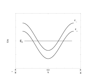
FIG. 1.: Dispersion relation for the two-band tight-binding model

The Fermi momentum for each band is defined through the equation

$$\epsilon^{(+)}(k_{F}^{(+)})=\epsilon^{(-)}(k_{F}^{(-)}).$$ (23)

The local constraint in eq. (3) leads to the global constraint $N^{(+)}+N^{(-)}=2N$, where $N^{(\pm)}$ is the occupation number operator for each band. Besides, $N^{(\pm)}=\frac{2Na}{\pi}k^{(\pm)}_{F}$. We thus obtain

$$\cos(k_{F}^{(-)}a)=\frac{t^{\prime}}{t}=\frac{J^{\prime}B^{\prime}_{0}}{2JB_{0}}$$ (24)

$$k_{F}^{(+)}=\pi/a-k_{F}^{(-)},$$ (25)

these implying

$$\epsilon^{(+)}(k_{F}^{(+)})=\epsilon^{(-)}(k_{F}^{(-)})=0.$$ (26)

The values of $t$ and $t^{\prime}$ are now determined by minimizing the energy of (20) under half-filling conditions,

$$E_{mf} = -\frac{L}{2\pi}\int_{-k_{F}^{(+)}}^{k_{F}^{(+)}}(2t\cos(ka)+2t^{\prime})\,2\,dk-\frac{L}{2\pi}\int_{-k_{F}^{(-)}}^{k_{F}^{(-)}}(2t\cos(ka)-2t^{\prime})\,2\,dk$$ (28)

$$+\frac{4L}{aJ}t^{2}+\frac{8L}{aJ^{\prime}}{t^{\prime}}^{2}.$$

Notice that $t<0$ just inverts the cosine curves, translating the Brillouin zone considered in $\pi/a$, and $t^{\prime}<0$ would just trade the roles of the two bands. Then, the relevant sector in the $t,t^{\prime}$ plane is $t\geq 0$ and $t^{\prime}\geq 0$. In this sector, the expression for the energy is

$$\frac{a\pi}{L}E_{mf}=-8t\sin(k_{F}^{(-)}a)-4t^{\prime}(\pi-2k_{F}^{(-)}a)+\frac{4\pi}{J}t^{2}+\frac{8\pi}{J^{\prime}}{t^{\prime}}^{2},~{}~{}~{}~{}~{}~{}~{}t^{\prime}<t,$$ (29)

and

$$\frac{a\pi}{L}E_{mf}=-4\pi t^{\prime}+\frac{4\pi}{J}t^{2}+\frac{8\pi}{J^{\prime}}{t^{\prime}}^{2},~{}~{}~{}~{}~{}~{}~{}~{}~{}~{}~{}~{}~{}~{}~{}~{}~{}~{}~{}~{}~{}~{}~{}~{}~{}~{}~{}~{}~{}~{}~{}~{}~{}~{}~{}~{}~{}~{}t^{\prime}>t.$$ (30)

The analysis of the above equations shows that, for $J^{\prime}<8/\pi^{2}~{}J$, the MF configuration depicts two bands which coincide with those corresponding to two decoupled chains ($t=J/\pi$, $t^{\prime}=0$), with Fermi momentum $k_{F}=k_{F}^{(-)}=k_{F}^{(+)}=\pi/(2a)$. Notice that the condition in eq. (17) holds and the linearization procedure around this minimum is valid.

On the contrary, for $J^{\prime}>\frac{8}{\pi^{2}}J$, we find that the global energy minimum corresponds to the point $t=0$, $t^{\prime}=J^{\prime}/4$ where the condition in eq. (17) does not hold (notice that there is still another local minimum while $J^{\prime}<2J$). The system in this configuration, which describes the strong coupling phase, presents a finite energy gap to spin excitations.

In the following two sections we will explore the $J^{\prime}<8/\pi^{2}~{}J$ region.

III Fluctuations and constraints: the $SU(4)_{1}/U(1)$ coset theory

In this section we take the continuum limit of the MF Hamiltonian in eq. (16) and then include fluctuations around MF and constraints in eq. (3). The outcome of this procedure is a perturbed $SU(4)_{1}/U(1)$ coset theory.

A Low-energy linearization in the thermodynamical continuum limit

In the region we consider ($J^{\prime}<8/\pi^{2}J$) the mean-field dispersion relation consists of two coinciding bands of amplitude $2J/\pi$. Linearization of low-energy excitations can be done around $k_{F}=\pi/(2a)$ in the usual way. The bandwidth will limit the validity of the resulting effective Field Theory to energies much smaller than $J$, independently of $J^{\prime}$.

Low-energy excitations in the thermodynamical continuum limit of the tight-binding model at half filling can be linearized in terms of Dirac fermions [11]. Fermionic position space operators $c^{(\pm)}$ for each band are readily written in terms of Dirac fermions $\psi^{(\pm)}(x)$ as

$$c^{(+)}_{n,\alpha}=\sqrt{a}(\exp(-ik_{F}x)\psi^{(+)}_{R,\alpha}(x)+\exp(ik_{F}x)\psi^{(+)}_{L,\alpha}(x)),$$ (31)

$$c^{(-)}_{n,\alpha}=\sqrt{a}(\exp(-ik_{F}x)\psi^{(-)}_{R,\alpha}(x)+\exp(ik_{F}x)\psi^{(-)}_{L,\alpha}(x)).$$ (32)

Here $\psi^{(+)}_{R,\alpha}$ and $\psi^{(+)}_{L,\alpha}$ stand for the right and left components of a Dirac spinor $\Psi^{(+)}_{\alpha}$ and so on. Dirac gamma matrices are taken as $\gamma_{0}=\sigma_{1}$, $\gamma_{1}=\sigma_{2}$. Notice that there is a total of four Dirac fermion species; using the notation $\alpha=\uparrow,\downarrow$ they are $(+,\uparrow),(-,\uparrow),(+,\downarrow),(-,\downarrow)$, which will be respectively denoted $\Psi_{i}(x)$, with $i=1,2,3,4$. Summation over repeated fermion species indices will be understood.

We arrive then at the linearized MF Hamiltonian

$$H_{mf}=v_{F}\int dx\bar{\Psi}_{i}(x)\gamma_{1}\partial_{x}\Psi_{i}(x),$$ (33)

where

$$v_{F}=2ta\sin(k_{F}a)=2Ja/\pi$$ (34)

is the Fermi velocity, and $\bar{\Psi}_{i}=\Psi^{\dagger}_{i}\gamma_{0}$. All four $\Psi$-fields have the same Fermi velocity, then the model, up to this point, possesses a manifest $U(4)$ symmetry.

B Fluctuations around mean field

We include now the fluctuation fields $B^{(1)}_{n},B^{(2)}_{n},B^{\prime}_{n}$. As we look for the continuum limit of the Hamiltonian (6), we will keep only relevant powers in $a$, as compared with eq. (33).

In order to keep track of $a$ orders, it is useful to make explicit the order $a$ contribution of fermion bilinears by defining

$$\begin{array}[]{l}z^{(1)}_{n}=a^{-1}c^{\dagger(1)}_{n,\alpha}c^{(1)}_{n+1,\alpha},\\ z^{(2)}_{n}=a^{-1}c^{\dagger(2)}_{n,\alpha}c^{(2)}_{n+1,\alpha},\\ z^{(3)}_{n}=a^{-1}c^{\dagger(1)}_{n,\alpha}c^{(2)}_{n,\alpha},\end{array}$$ (35)

so that the leading order for each $z$ is $a^{0}$. Notice that $z^{(1)}$ and $z^{(2)}$ still have to be expanded, as $(n+1)a=x+a$; the only relevant term in this expansion is that linear in $a$, containing first derivatives of $\psi$-fields. Our notation will be

$$z^{(i)}_{n}=w^{(i)}_{n}+av^{(i)}_{n}$$ (36)

(notice that $v^{(3)}_{n}=0$).

The relevant expansions for the $B$-fields, taking into account that the MF value of ${B^{\prime}}_{0}$ vanishes, are

$$\begin{array}[]{l}B^{(l)}_{n}=B_{0}+iaB_{0}A^{(l)}_{n}+aB_{0}R^{(l)}_{n}+O(a^{2}),\ \ \ \ (l=1,2)\\ {B^{\prime}}_{n}=iaA^{\prime}_{n}+aR^{\prime}_{n}+O(a^{2}).\end{array}$$ (37)

In particular, the terms quadratic in $B$ must be expanded as

$$\begin{array}[]{l}B^{\dagger(l)}_{n}B^{(l)}_{n}=B_{0}^{2}+2aB_{0}^{2}R^{(l)}_{n}+2a^{2}B_{0}^{2}{R^{(l)}}^{2}_{n},\ \ \ \ (l=1,2)\\ B^{{}^{\prime}\dagger}_{n}B^{\prime}_{n}=a^{2}{A^{\prime}}^{2}_{n}+a^{2}{R^{\prime}}^{2}_{n}.\end{array}$$ (38)

Using all of these, and making explicit the sums over $l=1,2$, the effective low energy Hamiltonian for (6) is written as

$$H_{eff}=H^{(1)}+H^{(2)}+H^{(3)}+O(a^{3})$$ (39)

where

$$H^{(1)} = \frac{J}{2}NB_{0}^{2}+\frac{J}{2}\sum_{n=1}^{N}aB_{0}(z^{(1)}_{n}+z^{\dagger(1)}_{n})+\frac{J}{2}\sum_{n=1}^{N}ia^{2}B_{0}A^{(1)}_{n}(w^{(1)}_{n}-w^{\dagger(1)}_{n})+$$ (41)

$$\frac{J}{2}\sum_{n=1}^{N}a(aB_{0}R^{(1)}_{n}(w^{(1)}_{n}+w^{\dagger(1)}_{n})+2B^{2}_{0}R^{(1)}_{n}+2aB^{2}_{0}{R^{(1)}}^{2}_{n}),$$

$$H^{(2)} = \frac{J}{2}NB_{0}^{2}+\frac{J}{2}\sum_{n=1}^{N}aB_{0}(z^{(2)}_{n}+z^{\dagger(2)}_{n})+\frac{J}{2}\sum_{n=1}^{N}ia^{2}B_{0}A^{(2)}_{n}(w^{(2)}_{n}-w^{\dagger(2)}_{n})+$$ (43)

$$\frac{J}{2}\sum_{n=1}^{N}a(aB_{0}R^{(2)}_{n}(w^{(2)}_{n}+w^{\dagger(2)}_{n})+2B^{2}_{0}R^{(2)}_{n}+2aB^{2}_{0}{R^{(2)}}^{2}_{n}),$$

$$H^{(3)} = \frac{J^{\prime}}{2}\sum_{n=1}^{N}ia^{2}[A^{\prime}_{n}(w^{(3)}_{n}-w^{\dagger(3)}_{n})+{A^{\prime}}^{2}_{n}]+$$ (45)

$$\frac{J^{\prime}}{2}\sum_{n=1}^{N}a^{2}[R^{\prime}_{n}(w^{(3)}_{n}+w^{\dagger(3)}_{n})+{R^{\prime}}^{2}_{n}]$$

The main things to notice here are:

- there are irrelevant (divergent) constant terms. This is expected from the combination of Hubbard-Stratonovich and MF techniques.

- the terms without fluctuations in $H^{(1)}$ and $H^{(2)}$ provide the two decoupled chains MF results discussed in the previous section.

- The $A^{(1)}$ and $A^{(2)}$ fields act as Lagrange multipliers; their total contribution to the effective action in the continuum limit reduces to a term

$$-i\frac{v_{F}}{2}\int dx\left((\bar{\Psi}_{i}(x)\gamma_{1}\Psi_{i}(x))(A^{(1)}(x)+A^{(2)}(x))+(\bar{\Psi}_{i}(x)\gamma_{1}(\sigma_{1}\otimes 1)_{ij}\Psi_{j}(x))(A^{(1)}(x)-A^{(2)}(x))\right)\ .$$ (46)

In the notation of eq. (46) the first matrix ($\sigma_{1}$) refers to isospin indices $(+),(-)$, while the second one ($1$) refers to spin indices $\uparrow,\downarrow$.

- The presence of a quadratic term in the ${A^{\prime}}$ field, with proper sign, allows for a trivial Gaussian integration. The same can be done with the $R$ fields. These of course brings back the original spin-spin rung interactions. In the present scheme their contribution includes quadratic terms in the $c$ operators, that lead to a redefinition of the Fermi velocity $v_{F}\rightarrow v_{F}/2$, and quartic perturbations that can be arranged as

$$-\frac{Ja^{2}}{16}\sum_{n=1}^{N}\left((w^{(1)}_{n}+w^{\dagger(1)}_{n})^{2}+(w^{(2)}_{n}+w^{\dagger(2)}_{n})^{2}\right)-\frac{J^{\prime}a^{2}}{2}\sum_{n=1}^{N}w^{(3)}_{n}w^{\dagger(3)}_{n}.$$ (47)

The continuum form of these quartic perturbations in terms of Dirac fermions is lengthy. We will write them down below, after introducing a convenient notation.

We notice that, for $J^{\prime}<8/\pi^{2}~{}J$, our approach leads to a description of the system which is the same as the one obtained in perturbative treatments, in principle valid for $J^{\prime}\ll J$ [4, 12]. In particular, the first two terms in (47) give rise to the well known marginally irrelevant perturbation terms in the individual chains. However, our approach does not rely on any perturbative treatment of $J^{\prime}$ and in particular allows for the determination of the phase diagram of the system, i.e. it predicts a critical value of the ratio $J^{\prime}/J$ which separates the two different regimes in the two-leg ladder. The situation is depicted in Fig. 2.

FIG. 2.: Phase diagram of the spin ladder. Bold bonds correspond to non zero links in the MF approximation.

Moreover, we show in the next section that the weak coupling structure unraveled in [4] arises naturally within our approach.

C Constraints

In this section we express the constraints (3) in terms of the linearized fermion fields and discuss how to implement them in the evaluation of the partition function for the spin ladder.

In the continuum limit the constraint on the occupation number at each site $(l),n$ separates in four parts, corresponding to oscillating and non-oscillating terms associated to each band. They read:

$$\bar{\Psi}_{i}\gamma_{0}\Psi_{i}=constant$$ (48)

which, implemented through a Lagrange multiplier $a_{0}$, provides the time component of a gauge field implementing a diagonal $U(1)$ coset constraint, $a_{\mu}=(a_{0},A^{(1)}+A^{(2)})$;

$$\bar{\Psi}_{i}\gamma_{0}(\sigma_{1}\otimes 1\!\!1)_{ij}\Psi_{j}=0$$ (49)

which, implemented through a Lagrange multiplier $b_{0}$, provides the time component of a second gauge field implementing the isospin $U(1)$ coset constraint, $b_{\mu}=(b_{0},A^{(1)}-A{(2)})$. These last two constraints

$$\bar{\Psi}_{i}\Psi_{i}=0;$$ (50)

$$\bar{\Psi}_{i}(\sigma_{1}\otimes 1\!\!1)_{ij}\Psi_{j}=0\ ,$$ (51)

lead to marginally irrelevant quartic perturbation terms when implemented through

$$\delta({\cal O}(x))\propto\lim_{\eta\rightarrow\infty}e^{-\eta{\cal O}^{\dagger}(x){\cal O}(x)},$$ (52)

just as in the case of decoupled chains.

To conclude this section, we collect all the terms in the effective low energy Hamiltonian which finally reads

$$H_{eff}=\frac{aJ}{\pi}\int dx~{}\bar{\Psi}_{i}(x)\left(\left(\gamma_{1}\partial_{x}-i\gamma_{\mu}a_{\mu}\right)\delta_{ij}-i\gamma_{\mu}(\sigma_{1}\otimes 1\!\!1)_{ij}b_{\mu}\right)\Psi_{j}(x)+\Delta H_{eff}\ ,$$ (53)

where $\Delta H_{eff}$ includes quartic terms in fermionic fields, which arise from (47) and (50),(51).

Clearly, the unperturbed theory posses a $U(4)$ symmetry which is gauged by a diagonal $U(1)$ field ($a_{\mu}$) and an isospin $U(1)$ field ($b_{\mu}$) which leads to the coset

$$\frac{U(4)}{U(1)_{diag}\times U(1)_{iso}}=\frac{SU(4)_{1}}{U(1)_{iso}},$$ (54)

where $SU(4)_{1}$ stands for the level $k=1$ WZW theory [13, 14].

Before displaying the explicit expression for the perturbations it is worth discussing in more detail the coset structure of the quadratic part of the Hamiltonian.

IV $SU(2)_{2}\times Z_{2}$ embedding, the perturbations in a new language

As it is known, the coset CFT $SU(4)_{1}$ can be alternatively described through the embedding [15]

$$SU(4)_{1}=SU(2)_{2}\times SU(2)_{2}\ .$$ (55)

The conformal central charges of the two theories coincide and primary fields in the $SU(4)_{1}$ can be written in terms of primaries in the two $SU(2)_{2}$ sectors. This will presently prove to be useful in the treatment of the perturbations. The different $SU(2)_{2}$ sectors in this embedding are naturally identified in eq. (53) as the spin and isospin sectors, in virtue of the $\sigma_{1}\otimes 1\!\!1$ non-diagonal structure. Moreover, in this language the second Lagrange multiplier $b_{\mu}$ gauges a $U(1)$ subgroup of the isospin $SU(2)_{2}$ sector giving rise to

$$SU(2)_{2}^{spin}\times SU(2)_{2}^{isospin}/U(1)^{isospin}=SU(2)_{2}^{spin}\times Z_{2}.$$ (56)

The last factor has been identified in [4] from the $Z_{2}$ structure of a two chain system.

All of this is most easily shown in the bosonized version of the coset CFT. To this end we write fermion bilinears as [13, 16]

$$\psi^{\dagger~{}i}_{R}\psi^{\bar{\jmath}}_{L}=M\Phi_{\Box}^{i{\bar{\jmath}}}$$ (57)

where $M$ is a renormalization constant and we have introduced bar indices in order to distinguish components transforming in the right and left fundamental representations of $SU(4)_{1}$. The $\Box$ subindex indicates the fundamental representation in the standard Young tableaux notation. In identifying the two $SU(2)_{2}$ sectors we find useful to keep the original spin and isospin (band) indices, writing

$$\Phi_{\Box}^{i{\bar{\jmath}}}=\Phi_{\Box}^{a\alpha,\bar{b}\bar{\beta}}$$ (58)

where we now use $a,\bar{b}$ for $(+),(-)$.

This field $\Phi_{\Box}^{i{\bar{\jmath}}}$ has scaling dimension $3/4$ and its components can be written in terms of products of the components of the fields in the fundamental representations of the two $SU(2)_{2}$ sectors as

$$\Phi_{\Box}^{a\alpha,\bar{b}\bar{\beta}}=\phi_{\Box}^{a,\bar{b}}{\phi}_{\Box}^{{}^{\prime}\alpha,\bar{\beta}}$$ (59)

where $\phi_{\Box}$ and ${\phi^{\prime}}_{\Box}$ are the primary fields in the fundamental (spin 1/2) representation of the two $SU(2)_{2}$ isospin and spin sectors respectively. These fields have scaling dimension $3/8$ so the product has the right dimension $3/4$ and moreover, correlation functions of the fields on both sides coincide.

The other primary field in the $SU(4)_{1}$ CFT is the one transforming in the antisymmetric ($6\times\bar{6}$) representation, which in the Young tableaux notation should read $\Phi_{\stackrel{{\scriptstyle\textstyle{\Box}}}{{\Box}}}$. It is built up from the antisymmetric product of two fields in the fundamental representation

$$\Phi_{\stackrel{{\scriptstyle\textstyle{\Box}}}{{\Box}}}={\cal A}\left(\Phi_{\Box}\Phi_{\Box}\right)$$ (60)

This field has scaling dimension $1$ and can be mapped into $SU(2)_{2}$ fields as

$$\Phi_{\stackrel{{\scriptstyle\textstyle{\Box}}}{{\Box}}}^{[(a_{1}\alpha_{1}),(a_{2},\alpha_{2})],[(\bar{b}_{1}\bar{\beta}_{1}),(\bar{b}_{2},\bar{\beta}_{2})]}=\phi_{\Box\!\Box}^{\{a_{1}a_{2}\},\{\bar{b}_{1}\bar{b}_{2}\}}\epsilon^{\alpha_{1}\alpha_{2}}\epsilon^{\bar{\beta}_{1}\bar{\beta}_{2}}+\epsilon^{a_{1}a_{2}}\epsilon^{\bar{b}_{1}\bar{b}_{2}}\phi_{\Box\!\Box}^{{}^{\prime}\{\alpha_{1}\alpha_{2}\}\{\bar{\beta}_{1}\bar{\beta}_{2}\}}$$ (61)

where $\phi_{\Box\!\Box},\phi_{\Box\!\Box}^{\prime}$ are the primary fields in the symmetric (spin 1) representations of the two $SU(2)_{2}$ sectors, which have the correct scaling dimension 1. In eq. (61) we have used the symbols $\{,\}$ and $[,]$ to indicate respectively symmetrization and antisymmetrization of indices.

We are now ready to analyze the different perturbation terms in $\Delta H_{eff}$. First of all, contribution coming from intrachain couplings and constraints are known to be marginally irrelevant, just as in the case of decoupled chains [8].

The interchain perturbation terms in $\Delta H_{eff}$ (those arising from the last term in (47)) can be separated into two groups according to their scaling dimensions: there are terms which correspond to relevant operators (scaling dimension 1) which can be identified with certain linear combination of the components of the primary (60) in the coset theory (53) and current-current terms, which have scaling dimension 2 and are hence marginal.

More precisely, for the relevant part we can write

$$\mbox{relevant perturbations}=-\lambda\int dx\left(\mbox{Tr}\left(A\Phi_{\stackrel{{\scriptstyle\textstyle{\Box}}}{{\Box}}}\right)+H.c.\ \right)\ ,$$ (62)

where $\lambda\propto J^{\prime}$ and $A$ is given by

$$A=\left(\begin{array}[]{cccccc}-1&0&0&0&0&0\\ 0&1/2&0&0&-1/2&0\\ 0&0&-1/2&1/2&0&0\\ 0&0&1/2&-1/2&0&0\\ 0&-1/2&0&0&1/2&0\\ 0&0&0&0&0&-1\end{array}\right)$$ (63)

(see the Appendix for details). Using the identifications described above and after some straightforward algebra we can readily identify the perturbation terms (62) in the embedding theory as

$$\mbox{relevant perturbations}=-\lambda\int dx\mbox{Tr}\left(\phi_{\Box\!\Box}+H.c.\right)+\frac{\lambda}{2}\int dx\mbox{Tr}\left(\phi^{\prime}_{\Box}\sigma_{1}\phi_{\Box}^{{}^{\prime}\dagger}\sigma_{1}+H.c.\right)$$ (64)

To analyze the effect of these perturbation terms it is convenient to reformulate the $SU(2)_{2}$ WZW sector in terms of three decoupled Majorana fermions, and in this new language it is easy to see that the first term gives a mass to all three Majorana fields [17]. The second one is simply the energy operator of the remaining Majorana sector [14, 18]. Being all perturbations of dimension $1$ we see that the gap opens linearly with the interchain coupling as predicted from the weak coupling limit [3, 4]. Note the different sign in the masses of the two sectors, also in agreement with the weak coupling analysis.

As for the current-current terms, they correspond to marginal perturbations and can be written as

$$\mbox{marginal perturbations}=-\frac{aJ^{\prime}}{8}\int dx\left(-\psi^{\dagger}_{L}((\sigma_{3}+i\sigma_{2})\otimes 1\!\!1)\psi_{L}\psi^{\dagger}_{L}((\sigma_{3}-i\sigma_{2})\otimes 1\!\!1)\psi_{L}-R\leftrightarrow L\right)$$ (65)

$$-\frac{aJ^{\prime}}{8}\int dx\left(\psi^{\dagger}_{L}((\sigma_{3}+i\sigma_{2})\otimes 1\!\!1)\psi_{L}\psi^{\dagger}_{R}((\sigma_{3}-i\sigma_{2})\otimes 1\!\!1)\psi_{R}+R\leftrightarrow L\right)$$ (66)

$$-\frac{aJ^{\prime}}{8}\int dx\left(-\psi^{\dagger}_{L}(1\!\!1\otimes 1\!\!1)\psi_{L}\psi^{\dagger}_{R}(1\!\!1\otimes 1\!\!1)\psi_{R}-\psi^{\dagger}_{L}(1\!\!1\otimes\vec{\sigma})\psi_{L}.\psi^{\dagger}_{R}(1\!\!1\otimes\vec{\sigma})\psi_{R}\right)$$ (67)

$$-\frac{aJ^{\prime}}{8}\int dx\left(\psi^{\dagger}_{L}(\sigma_{1}\otimes 1\!\!1)\psi_{L}\psi^{\dagger}_{R}(\sigma_{1}\otimes 1\!\!1)\psi_{R}+\psi^{\dagger}_{L}(\sigma_{1}\otimes\vec{\sigma})\psi_{L}.\psi^{\dagger}_{R}(\sigma_{1}\otimes\vec{\sigma})\psi_{R}\right)$$ (68)

The first two terms (first line) renormalize the Fermi velocity of the Majorana (isospin) sector, while the third and fourth (second line) correspond to marginal forward-scattering terms in the same sector. The fifth and seventh terms are effectively zero due to the constraints on the two corresponding $U(1)$ currents and the sixth term correspond to the marginal forward-scattering terms in the spin sector. The very last one mixes spin and isospin sectors. This last contribution is nevertheless marginal, so it does not change the low energy physics which in the present case is dominated by the relevant perturbations already discussed. Its effect could be important in the analysis of e.g. zig-zag ladders where the relevant perturbations are wiped out, as we show in the next Section, and only marginal interactions play a rôle [19, 20, 21, 22].

It can be easily shown that the marginal terms which are present on each separate chain, written in the present language correspond to the sixth and eight terms in the above expression. Due to the fact that these terms correspond to marginally irrelevant couplings and that they form a closed algebra, they will have no effect in the low energy dynamics whatsoever. After having observed that, one can see that the effective theory consists of two sectors which are decoupled from each other.

V Other structures: crossed and zig-zag ladders

In this section we will extend our previous analysis to more general situations, which are not only of academic interest, but are relevant in the analysis of real materials. These more general situations arise when other (diagonal) couplings between spins in neighbouring chains are not negligible. The two structures that we analyze now are the so-called crossed ladders [23, 25], in which couplings along the two diagonals are added, and zig-zag ladders in which only one diagonal coupling is added [19, 20, 21, 22]. Another potential application of the present formalism would be the study of the interplay between interchain coupling and dimerization along the legs [26, 27, 28].

i) Crossed ladders

We consider a Heisenberg Hamiltonian given by

$$H=\sum_{n=1}^{N}\sum_{l=1}^{2}J{\vec{S}}^{(l)}_{n}.{\vec{S}}^{(l)}_{n+1}+J^{\prime}\sum_{n=1}^{N}{\vec{S}}^{(1)}_{n}.{\vec{S}}^{(2)}_{n}+J_{\times}\sum_{n=1}^{N}\left({\vec{S}}^{(1)}_{n}.{\vec{S}}^{(2)}_{n+1}+{\vec{S}}^{(1)}_{n+1}.{\vec{S}}^{(2)}_{n}\right)\ .$$ (69)

where the last term corresponds to additional diagonal couplings.

Following the same approach as for the normal ladder we introduce Hubbard-Stratonovich fields associated to each coupling and perform a three-parameter MF analysis proposing constant values for the intrachain couplings, the interchain (rung) coupling and the interchain (diagonal) couplings. We find two different regions in the parameter space $(J/J^{\prime},J_{\times}/J^{\prime})$. It should be noted that this Hamiltonian is dual under the interchange $J\leftrightarrow J_{\times}$, then it is enough to study the region $J_{\times}\leq J$.

(a) If $J/J^{\prime}>\pi^{2}/8$, the MF analysis yields the system in a weak coupling regime, and following all the same steps as before, we arrive at the same effective Field Theory with the noticeable change that the coefficient of the relevant perturbations is now shifted as $J^{\prime}-2J_{\times}$. As in the weak coupling analysis [23, 24], one immediately sees that there is a line in which the relevant perturbations vanish. On this line one could expect a massless regime, as suggested by numerical studies [23, 25]. However in a recent treatment of the resulting bosonized Hamiltonian it was shown that the current-current terms are marginally relevant and a gap opens [24]. The same conclusion is attained in our resulting effective theory. Again, the new feature here is that we find the region of validity of the weak coupling effective Field Theory to go up to $J^{\prime}=8/\pi^{2}J$.

(b) If $J/J^{\prime}<\pi^{2}/8$, the system falls in a strong coupling regime in which the two dispersion bands are separated by a gap ($\propto J^{\prime}$) and then a low-energy effective Field Theory description is not suitable here.

FIG. 3.: Phase diagram of the crossed ladder. Bold bonds correspond again to non zero links in the MF approximation.

ii) Zig-zag ladders

The Hamiltonian is given by

$$H=\sum_{n=1}^{N}\sum_{l=1}^{2}J{\vec{S}}^{(l)}_{n}.{\vec{S}}^{(l)}_{n+1}+J^{\prime}\sum_{n=1}^{N}{\vec{S}}^{(1)}_{n}.\left({\vec{S}}^{(2)}_{n}+{\vec{S}}^{(2)}_{n+1}\right)\ .$$ (70)

Introducing again Hubbard-Stratonovich fields associated to each coupling and performing a MF analysis with constant values for the intrachain and interchain couplings, we find a different situation: while we still find a regime, which now exists for $J^{\prime}<J$, in which we re-obtain the standard weak coupling results, we find that the “strong coupling” regime, ($J^{\prime}>J$), can still be described by an effective low energy Field Theory.

More precisely, in the regime in which $J^{\prime}<J$ we find that all relevant perturbations cancel in a way similar to that found in the weak coupling limit [19, 20, 21, 22]. The effective low energy theory corresponds to the same coset theory, perturbed only by the operators appearing in the first, third and fourth lines in eq. (68). The so-called parity breaking terms first studied in [21] appear in the present approach from the next-to-leading order in the lattice-spacing $a$ in the expansion of the modified version of (47).

In the other regime, ($J^{\prime}>J$), the bands at the MF minimum are given by

$$\epsilon^{(+)}(k) = -\frac{J^{\prime}}{\pi}\sqrt{2(1+\cos(ka))},$$ (71)

$$\epsilon^{(-)}(k) = \frac{J^{\prime}}{\pi}\sqrt{2(1+\cos(ka))}\ ,$$ (72)

being no gap between them, and a Field Theory description is still possible. The difference is that the low energy effective theory should in this case be built up on only two fermion species, exhibiting $SU(2)_{1}$ symmetry. This should correspond to the description of a single chain plus next-nearest-neighbour interactions, which is the suitable picture for the regime where $J^{\prime}$ dominates.

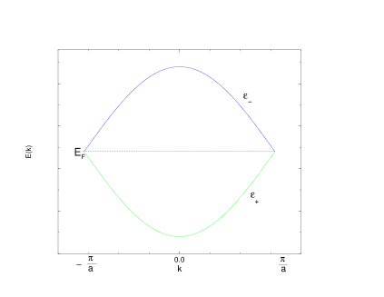
FIG. 4.: Energy bands for the zig-zag ladder at $J^{\prime}>J$ MF minimum

Once again, our method allows for the construction of an effective field Theory for the full range of couplings and in particular would allow to study the transition from the massless ($c=1$) $J=0$ limit to the massive Kosterlitz-Thouless regime known to arise at $J\approx 0.24J^{\prime}$ [29], which should, according to our analysis, extend to the limit $J^{\prime}\rightarrow 0$.

FIG. 5.: Phase diagram of the zig-zag ladder. Bold bonds correspond again to non zero links in the MF approximation.

Since the main purpose of the present paper is to emphasize the potential applications of our approach, the analysis of these effective field theories will be addressed in a separate publication.

VI Conclusions

The approach developed in the present paper shows that the spectrum predicted from weak coupling approximation extends up to a finite value of $J^{\prime}/J$, our estimation of this critical value being $\frac{J^{\prime}_{c}}{J}\sim\frac{8}{\pi^{2}}$. Beyond this value our MF analysis of Section II predicts a cross-over to the strong coupling regime, where the rungs of the ladder become disconnected among them. Fluctuations over this state will restore connectivity and the strong coupling approach of [30, 31] would be the appropriate starting point in this parameter regime. As the classical potential analyzed in Section II has a double well structure in the intermediate region ($J^{\prime}\sim J^{\prime}_{c}$) we expect a smooth cross-over from weak to strong coupling regime. Experimental observation of this cross-over supposes the variation of the ratio of the exchange parameter. This could in principle be achieved by applying pressure in the perpendicular direction of the ladder axis.

Though our approach starts from a MF analysis, fluctuations are taken into account to all orders. Besides, it allows for a classification of all the perturbations in the language of the embedding of the theory into $SU(2)_{2}\times Z_{2}$. One interesting observation which arises is that only the $Z_{2}$ Majorana Fermi velocity is renormalized to first order in $J^{\prime}$ by the interacions.

The study of hole doped spin ladders is a natural extension of our approach. For this case the $t-J$ model should be considered and the charge sector of the theory could be represented by a spinless boson (the slave boson representation). However the magnetic excitations will evolve from the triplet and the singlet found in this paper. The question of the hole pairing due to these excitations could therefore be addressed within our formalism. This will be reported elsewhere.

Acknowledgements: We are grateful to E.F. Moreno for useful discussions and computational help. We thank A. Greco, A. Honecker, A.A. Nersesyan and P. Pujol for useful comments. We thank CONICET and Fundación Antorchas (grants No. A-13622/1-106 and A-13740/1-64) for financial support.

Appendix

We write in this appendix the explicit form of some lengthy expressions appearing with compact notation in the main text.

The relevant part of the third term in eq. (47), appearing in eq. (53), reads in the continuum limit

$$\mbox{relevant perturbations}=$$ (73)

$$- \frac{J^{\prime}a}{2}\int dx\left(-\Psi^{\dagger(-)}_{R,\alpha}\Psi^{\dagger(-)}_{R,\beta}\Psi^{(-)}_{L,\alpha}\Psi^{(-)}_{L,\beta}+\Psi^{\dagger(-)}_{R,\alpha}\Psi^{\dagger(-)}_{R,\beta}\Psi^{(-)}_{L,\alpha}\Psi^{(+)}_{L,\beta}-\Psi^{\dagger(-)}_{R,\alpha}\Psi^{\dagger(-)}_{R,\beta}\Psi^{(+)}_{L,\alpha}\Psi^{(-)}_{L,\beta}+\Psi^{\dagger(-)}_{R,\alpha}\Psi^{\dagger(-)}_{R,\beta}\Psi^{(+)}_{L,\alpha}\Psi^{(+)}_{L,\beta}\right.$$ (74)

$$- \Psi^{\dagger(-)}_{R,\alpha}\Psi^{\dagger(+)}_{R,\beta}\Psi^{(-)}_{L,\alpha}\Psi^{(-)}_{L,\beta}+\Psi^{\dagger(-)}_{R,\alpha}\Psi^{\dagger(+)}_{R,\beta}\Psi^{(-)}_{L,\alpha}\Psi^{(+)}_{L,\beta}-\Psi^{\dagger(-)}_{R,\alpha}\Psi^{\dagger(+)}_{R,\beta}\Psi^{(+)}_{L,\alpha}\Psi^{(-)}_{L,\beta}+\Psi^{\dagger(-)}_{R,\alpha}\Psi^{\dagger(+)}_{R,\beta}\Psi^{(+)}_{L,\alpha}\Psi^{(+)}_{L,\beta}$$ (75)

$$+ \Psi^{\dagger(+)}_{R,\alpha}\Psi^{\dagger(-)}_{R,\beta}\Psi^{(-)}_{L,\alpha}\Psi^{(-)}_{L,\beta}-\Psi^{\dagger(+)}_{R,\alpha}\Psi^{\dagger(-)}_{R,\beta}\Psi^{(-)}_{L,\alpha}\Psi^{(+)}_{L,\beta}+\Psi^{\dagger(+)}_{R,\alpha}\Psi^{\dagger(-)}_{R,\beta}\Psi^{(+)}_{L,\alpha}\Psi^{(-)}_{L,\beta}-\Psi^{\dagger(+)}_{R,\alpha}\Psi^{\dagger(-)}_{R,\beta}\Psi^{(+)}_{L,\alpha}\Psi^{(+)}_{L,\beta}$$ (76)

$$+ \left.\Psi^{\dagger(+)}_{R,\alpha}\Psi^{\dagger(+)}_{R,\beta}\Psi^{(-)}_{L,\alpha}\Psi^{(-)}_{L,\beta}-\Psi^{\dagger(+)}_{R,\alpha}\Psi^{\dagger(+)}_{R,\beta}\Psi^{(-)}_{L,\alpha}\Psi^{(+)}_{L,\beta}+\Psi^{\dagger(+)}_{R,\alpha}\Psi^{\dagger(+)}_{R,\beta}\Psi^{(+)}_{L,\alpha}\Psi^{(-)}_{L,\beta}-\Psi^{\dagger(+)}_{R,\alpha}\Psi^{\dagger(+)}_{R,\beta}\Psi^{(+)}_{L,\alpha}\Psi^{(+)}_{L,\beta}+H.c.\ \right)$$ (77)

by simple use of eqs. (31), (32), (35), (36).

The explicit form of eq. (60) in terms of fermions, using eq. (57), is

$$\Phi_{\stackrel{{\scriptstyle\textstyle{\Box}}}{{\Box}}}^{[(i_{1}\alpha_{1}),(i_{2},\alpha_{2})],[(\bar{\jmath}_{1}\bar{\beta}_{1}),(\bar{\jmath}_{2},\bar{\beta}_{2})]}={\cal A}\left(\Phi_{\Box}^{(i_{1}\alpha_{1}),(\bar{\jmath}_{1}\bar{\beta}_{1})}\Phi_{\Box}^{(i_{2},\alpha_{2}),(\bar{\jmath}_{2},\bar{\beta}_{2})}\right)\ ,$$ (78)

where antisymmetrization affects bar and unbar pairs of indices separately.

Using eqs. (77) and (78), expression (62) follows immediately. The base used for writing the matrix $A$ in eq. (63) is the one made explicit with indices in the l.h.s. of eq. (61), ordered as $[(+,\uparrow),(-,\uparrow)],[(+,\uparrow),(+,\downarrow)],[(+,\uparrow),(-,\downarrow)],[(-,\uparrow),(+,\downarrow)],[(-,\uparrow),(-,\downarrow)],[(+,\downarrow),(-,\downarrow)]$.

REFERENCES

• [1] For a recent review on the status of experimental results on ladders see E. Dagotto, preprint cond-mat/9908250.
• [2] T. Barnes, E. Dagotto, J. Riera and E.S. Swanson, Phys. Rev. B46, 3196 (1993).
• [3] K. Totsuka and M. Suzuki, J. Phys.: Condensed Matter 7, 6079 (1995).
• [4] D.G. Shelton, A.A. Nersesyan and A.M. Tsvelik, Phys. Rev. B53, 8521 (1996).
• [5] E. Orignac and R. Citro, Phys. Rev. B 62, 8622 (2000).
• [6] M.V. Abrashev, C. Thomsen and M. Surtchev, Physica C 280, 297 (1997).
• [7] J. Marston and I. Affleck, Phys. Rev. B39, 11538 (1989).
• [8] C. Itoi and H. Mukaida, J. Phys. A: Math. Gen. 27, 4695 (1994).
• [9] C. Mudry and E. Fradkin, Phys. Rev. B 50, 11409 (1994)
• [10] P.J. Freitas and R.R.P. Singh, Phys. Rev. B 62, 5525 (2000).
• [11] I. Affleck,in Fields, Strings and Critical Phenomena, Les Houches, Session XLIX, edited by E. Brezin and J. Zinn-Justin (North-Holland, Amsterdam, 1988).
• [12] Y. Hosotani, J. Phys. A 30 L757 (1997), Erratum A31, 7415 (1998).
• [13] E. Witten, Comm. Math. Phys. 94, 455 (1984).
• [14] V.G. Knizknik and A.B. Zamolodchikov, Nucl. Phys. B247, 83 (1984).
• [15] See e.g. P. Bouwknegt and K. Schoutens, Phys. Rep. 223, 183 (1993).
• [16] S.G. Naculich and H.J. Schnitzer, Nucl. Phys. B332, 583 (1990).
• [17] A.B. Zamolodchikov and V.A. Fateev, Sov. Phys. JETP 62, 215 (1985).
• [18] D.C. Cabra and E.F. Moreno, Nucl. Phys. B475, 522 (1996).
• [19] S.R. White and I. Affleck, Phys. Rev. B54, 9862 (1996).
• [20] D. Allen and D. Sénéchal, Phys. Rev. B55, 299 (1997).
• [21] A.A. Nersesyan, A.O. Gogolin and F.H.L. Eßler, Phys. Rev. Lett. 81, 910 (1998).
• [22] D.C. Cabra, A. Honecker and P. Pujol, Eur. Phys. J. B 13, 55 (2000).
• [23] Z. Weihong, V. Kotov and J. Oitmaa, Phys. Rev. B 57, 11439 (1998).
• [24] D. Allen, F.H.L. Essler and A.A. Nersesyan, Phys. Rev. B 61 (2000), 8871.
• [25] X. Wang, preprint cond-mat/9803290.
• [26] M.A. Martín-Delgado, R. Shankar and G. Sierra, Phys. Rev. Lett. 77, 3443 (1996).
• [27] D.C. Cabra and M.D. Grynberg, Phys. Rev.  Lett. 82, 1768 (1999).
• [28] Y.-J. Wang and A.A. Nersesyan, Nucl. Phys. B583, 671 (2000).
• [29] S. Eggert, Phys. Rev. B 54, R9612 (1996).
• [30] S. Sachdev and R.N. Bhatt, Phys. Rev. B41, 9323 (1990).
• [31] S. Gopalan, T.M. Rice and M. Sigrist, Phys. Rev. B49, 8901 (1996).