Invalidation of the Kelvin Force in Ferrofluids

Abstract

Direct and unambiguous experimental evidence for the magnetic force density being of the form $M{\boldsymbol{\nabla}}B$ in a certain geometry — rather than being the Kelvin force $M{\boldsymbol{\nabla}}H$ — is provided for the first time. ($M$ is the magnetization, $H$ the field, and $B$ the flux density.)

In studying polarizable and magnetizable condensed systems, one of a few key concepts is the force exerted by applied electric and magnetic fields. A clear and precise understanding here is therefore of crucial importance. For a neutral, dielectric body, this force is usually taken to be the Kelvin force LL ; si ; n1 ,

$${\boldsymbol{\cal F}}_{\rm K}=\int[P_{i}{\boldsymbol{\nabla}}E_{i}+\mu_{0}M_{i}{\boldsymbol{\nabla}}H_{i}]\,{\rm d}^{3}r,$$ (1)

where $P$ is the polarization, $M$ the magnetization, $E$ the electric and $H$ the magnetic field; $\mu_{0}$ and $\epsilon_{0}$ are as usual the vacuum permeability and permittivity, and the integral is over the volume of the body. (Summation over repeated indices is always implied.)

In spite of general believes, however, the theoretical foundation for this expression is far from rock solid, and recent considerations have pointed to the validity, under conditions to be specified below, of the variant expression rev

$${\boldsymbol{\cal F}}_{\rm v}=\int[(P_{i}/\epsilon_{0}){\boldsymbol{\nabla}}D_{i}+M_{i}{\boldsymbol{\nabla}}B_{i}]\,{\rm d}^{3}r,$$ (2)

where $\bf D\equiv\epsilon_{0}E+P$ and $\bf B\equiv\mu_{0}(H+M)$ are the dielectric displacement and magnetic flux density, respectively. This circumstance makes a direct measurement of the electromagnetic force desirable.

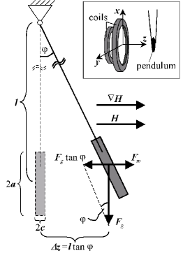
Figure 1: Schematic representation of the experiment, a pendulum deflected by a magnetic force. The inset shows the two magnetic coils producing the field. The object marked as pendulum is a disk containing ferrofluid, with its face perpendicular to both the field and field gradient.

In this Letter, such an experiment for the magnetic part of the force is reported. It consists of a pendulum exposed to a well defined, horizontal magnetic field with a gradient parallel to the field, see Fig. 1. The weight of the pendulum is a disk-shaped container. It is filled with ferrofluid and has its face aligned normal to the field. The disk is drawn by the field gradient, but leaves the applied field essentially unchanged. Given the careful design of the experiment, with especially the string of the pendulum close to 8 m, its displacement yields an easy and accurate measurement of the magnetic force. For the given geometry, Eq (2) was verified to great precision.

The quest for the correct form of the electromagnetic force sounds, and is indeed, vintage 19^th century. So it is truly amazing that something as elementary as the rest position of a pendulum subject to a static magnetic field cannot be predicted in general consensus even today. Kelvin was the first to have made a lasting contribution in this context by first calculating, microscopically, the force exerted by an external field on a single dipole, and then taking the total force as the sum of the forces on all dipoles. Clearly, this is only justified if the dipoles are too far apart to interact, if the system is electromagnetically dilute. This implies a small magnetization and susceptibility, $M\ll H$, $\chi\ll 1$. (We shall only be discussing the magnetic force from here on.) Part of the terms neglected must be quadratic in $M$, as they naturally account for interaction. Therefore, this approach cannot distinguish between Eq (1) and (2), the difference of which is $\frac{1}{2}\mu_{0}{\boldsymbol{\nabla}}M^{2}$, a term quadratic in $M$, or $\chi$.

The classic derivation of the electromagnetic force is thermodynamic in nature, and rather more generally valid, cf §15 and 35 of the book on macroscopic electrodynamics by Landau and Lifshitz  LL . Starting from the Maxwell stress tensor $\Pi_{ij}$, this derivation subtracts the hydrostatic “zero-field pressure” – the pressure that would be there in the absence of fields, for given temperature and density – and identifies the gradient of the rest as the electromagnetic (or Helmholz) force. If the susceptibility $\chi$ – irrespective of its value – is taken to be proportional to the density (or concentration of magnetic particles in a suspension such as ferrofluid), this expression reduces to the Kelvin force, Eq (1). With the difference between Eq (1) and (2) appreciable if $\chi\gtrsim 1$, this derivation may be taken to clearly rule out Eq (2).

Ferrofluids are stable suspensions of magnetic nano-particles, with an initial susceptibilities up to about 5 that are usually proportional to the volume concentration $\rho_{1}$ of magnetic particles at small fields, see Fig 2. It is therefore standard assumption that the Kelvin force, Eq (1), may be employed wherever $\chi\sim\rho_{1}$ holds rs .

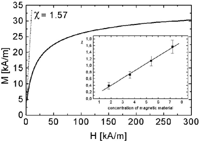
Figure 2: Magnetization of a typical ferrofluid (No 7 in Table 2) as a function of the field $H$. The inset shows the dependence of $\chi$ on the concentration of magnetic particles for four fluids of similar microscopic make-up, especially the mean particle diameter.

Closer examination luo , however, has raised doubts about the validity of Eq (1) for highly magnetizable systems, by unearthing an implicit assumption of small susceptibilities, made during the derivation as given by Landau and Lifshitz. So, in spite of appearance, neither does this derivation distinguish between Eq (1) and (2). Rather more important, however, is the fact that this force is not operative in equilibrium, when the divergence of the Maxwell stress vanishes, $\nabla_{j}\Pi_{ij}=0$, and the gradient of the zero field pressure compensates the Kelvin force.

Generally speaking, while the electromagnetic force is a simple and unique quantity in microscopic physics, given by the Lorentz force, it is a multi-faceted, heuristic concept in macroscopic physics. Not aware of this fact, and possibly for want of something better, we tend to take Eq (1) – with its curious preference of $E,H$ over $D,B$ – as the electromagnetic force. (There is of course also the macroscopic Lorentz force, which is however zero if the system is neutral and insulating).

To understand why this is a conceptual pitfall, consider the hydrodynamic theory for ordinary fluids, such as water or air, in the absence of fields. It consists of a set of partial differential equations including the Navier-Stokes equation LL6 . By solving these equations with the appropriate initial and boundary conditions, one is in principle able to predict any experimental outcome – say the trajectory of an airplane – without ever the need to introduce the concept of force. For the convenience of reasoning and arguing, however, we do label certain terms as force densities: in the differential equations, boundary conditions, or the solution under consideration. As a result, these forces depend on the context and geometry – take the form of the airfoil and the associated lift.

Circumstances are similar in the hydrodynamic theory of ponderable systems LL ; rev ; ml , and there is just as little reason to expect the existence of a unique electromagnetic force that is independent from geometry and context. But we do also need the concept of force: Physics does not comprise solely of mathematics, and clear thinking about the valid expressions for the electromagnetic force under given conditions will give us considerable heuristic power in prediction — without having to solve the set of partial differential equations each and every time. A simple question about the rest position of a pendulum subject to a field should be answerable by considering an elementary force equilibrium, between the strain in the string, the gravitational and the electromagnetic force. Solving the hydrodynamic theory with appropriate boundary conditions rev and assuming linear constitutive relation, the magnetic force is found to be

$${\boldsymbol{\cal F}}={\textstyle\frac{1}{2}}\oint[\mu_{0}\chi H{\rm{}_{t}}^{2}+\chi B{\rm{}_{n}}^{2}/(1+\chi)\mu_{0}]\,{\rm d}{\bf A},$$ (3)

where the surface integral is to be taken over the surface of the magnetizable body. The subscripts _t and _n denote the tangential and normal field component with respect to the surface. As the above fields are continuous across the interface, they may be both the external or the internal field. Eq (3) is rather generally valid. It holds irrespective of $\chi$’s size, or its dependency on either the density or the volume concentration of magnetic particles; it is also easily generalized for nonlinear constitutive relations. Equilibrium, however, is an essential requirement.

Employing the Gauss law, and provided $\chi$ is spatially constant, with $M=\chi H=$ $\chi B/\mu_{0}(1+\chi)$, we may rewrite Eq (3) as a volume integral,

$${\boldsymbol{\cal F}}=\int(\mu_{0}M_{\rm t}{\boldsymbol{\nabla}}H_{\rm t}+M{\rm{}_{n}}{\boldsymbol{\nabla}}B_{\rm n})\,{\rm d}^{3}r.$$ (4)

If the field is normal to the surface, as in the above experiment, the first term vanishes, and ${\boldsymbol{\cal F}}_{\rm v}$ of Eq (2) is retrieved; if the field is tangential to the surface, Eq (1) and ${\boldsymbol{\cal F}}_{\rm K}$ hold.

Casting doubts – however well theoretically founded – on the applicability of the Kelvin force certainly requires experimental validation. Fortunately, in strongly magnetizable systems such as ferrofluids, the difference between ${\boldsymbol{\cal F}}_{\rm K}$ and ${\boldsymbol{\cal F}}_{\rm v}$ is appreciable. For linear constitutive relations, the latter is larger by the factor $1+\chi$: With the magnetic field perpendicular to the disk surface, we have $B_{\rm in}=B_{\rm ex}$ $=\mu_{0}H_{\rm ex}$, where the subscripts _in and _ex denote the internal and external field, respectively. This implies $H_{\rm in}=$ $H_{\rm ex}/(1+\chi)$ and $M=\chi H_{\rm in}$ $=\chi H_{\rm ex}/(1+\chi)$. As the disk containing the ferrofluid is not infinite, the external field $H_{\rm ex}$ is not quite the applied field $H_{0}$. Approximating the disk as a (flat) ellipsoid, we may write $H_{\rm ex}/(1+\chi)$ $=H_{\rm in}=$ $H_{0}/(1+D\chi)$, where $D$ is the demagnetization factor. (The ferrofluid sample has the form of a flat disk with a diameter of $a=50$ mm, thickness $c=1$ mm, and $b\equiv a/c$ $=50$, from which the demagnetization factor in $z$ direction is calculated as $D=0.9694$, employing the approximation 5 $D=1-$ $\pi/2b$ $+2b^{2}$.) Inserting these formulas into Eqs (1) and (2), respectively, we find

$${\boldsymbol{\cal F}}_{\rm K}=[{\textstyle\frac{1}{2}}V\mu_{0}\chi/(1+D\chi)^{2}]{\boldsymbol{\nabla}}H_{0}^{2},$$ (5)

$${\boldsymbol{\cal F}}_{\rm v}=(1+\chi)[{\textstyle\frac{1}{2}}V\mu_{0}\chi/(1+D\chi)^{2}]{\boldsymbol{\nabla}}H_{0}^{2}.$$ (6)

They show ${\boldsymbol{\cal F}}_{\rm v}=(1+\chi){\boldsymbol{\cal F}}_{\rm K}$, and give the force in terms of simple, measurable quantities: susceptibility $\chi$, applied field $H_{0}$, the demagnetization factor $D$, and the ferrofluid volume $V$. (Due to the small gradient of the applied field, the volume integral was approximated by multiplication with $V$.)

The magnetic field, with its direction and gradient both parallel to the $z$-direction, is produced by an arrangement of two coils, which is simply half a Fanselau-arrangement 6 , see Fig. 1. The field is homogeneous in the $xy$-plane to an accuracy of better than 0.1 %. Both the field and its gradient are proportional to the applied current $I$. The field strength shows a quadratic decrease in $z$-direction, leading to a linear dependence of the field gradient. Choosing the center of the larger coil as the origin of the coordinate system ($z=0$ is at the outer edge of the coil), the field is parameterized with three coefficients, $\alpha_{1}=2.5\times 10^{4}{\rm m}^{-3}$, $\alpha_{2}=0.47$m, $\alpha_{3}=750{\rm m}^{-1}$, as

$$H_{0}=[\alpha_{1}(z-\alpha_{2})^{2}-\alpha_{3}]I.$$ (7)

($H_{0}$ denotes the $z$-component of the field. The other components are not zero for $z\not=0$, as ${\boldsymbol{\nabla}}\cdot{\bf B}=0$. The force density from the $x,y$-components of the field is quadratically small, and integrates to zero for a disk centered at $z=0$.)

The disk containing the ferrofluid is attached to two nylon strings, of length $l=7650$ mm and mounted to a tripod, forming a pendulum. The rest position of the pendulum is at $x,y=0$ and $z=7.6$ cm. If a magnetic field is applied, the magnetic force acting on the fluid attracts the disk towards the coils. This results in its displacement and, as shown in Fig. 1, a restoring gravitational force, the relevant component of which is $mg\tan\varphi$ $=mg\Delta z/l$, with $m$ the mass of the disk, $g$ the gravitational acceleration, $\varphi$ the angle of deflection, and $\Delta z$ the displacement. In equilibrium, the gravitational force is equal to the magnetic one, either ${\boldsymbol{\cal F}}_{\rm K}$ of Eq (5) or ${\boldsymbol{\cal F}}_{\rm v}$ of Eq (6), but always $\sim\nabla H_{0}^{2}$. Writing the magnetic force as $\beta\nabla H_{0}^{2}$ and equating it with $mg\Delta z/l$, we find

$$\Delta z=(\beta l/mg)\nabla H_{0}^{2}=\lambda H_{0}\nabla H_{0}.$$ (8)

The slope $\lambda\equiv 2\beta l/mg$ is measured by plotting $\Delta z$ over $H_{0}\nabla H_{0}$.

Due to the great length of the pendulum, even small changes of the magnetic force will provide easily measurable changes of $\Delta z$. For instance, a change of the magnetic force of $10^{-5}$N corresponds to $\Delta z=1$mm. In addition, since $\Delta z=13$ mm corresponds to $\varphi=0.1^{\circ}$, even relatively large displacements, of the order of a few cm, will not lead to a tilt of the disk relative to the field direction. This ensures the homogeneity, over the sample, of the magnetic field $H_{0}$ in x-direction. The position of the sample is monitored by a digital video system, allowing a determination of the displacement $\Delta z$ with an accuracy of approximately 0.2 mm.

With the experimental setup described above, we have carried out a series of experiments using 11 different ferrofluids having different initial susceptibility, ranging from 0.18 to approximately 4, cf table 2. (For ferrofluids supplied by Ferrofluidics, the trade names are given in table 2.) Because only weak magnetic fields up to a maximum of $H_{0}=10$kA/m are used in the experiment, the validity of linear constitutive relation is ensured, cf Fig 2, and we can use the initial susceptibility of table 2 throughout the evaluation of the data.

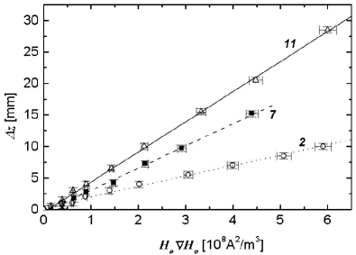
Figure 3: Dependence of the displacement $\Delta z$ of the pendulum on $H_{0}\nabla H_{0}$, for fluids 2, 7 & 11, with linear fits.

Fig. 3 shows the displacement $\Delta z$ of the disk as functions of $H_{0}\nabla H_{0}$, for three different fluids from table 2. It is obvious that the linear relation between $\Delta z$ and $H_{0}\nabla H_{0}$ is well satisfied over the whole range of investigation, attesting to the validity of the linear constitutive relation employed in the evaluation. From plots like these, we can determine the slope to an accuracy of about 3%. By averaging over five runs for each fluid, the accuracy is increased to approximately 1.5%, demonstrating the reproducibility of the data.

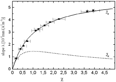
Figure 4: $\lambda=\Delta z/(H_{0}\nabla H_{0})$ as a function of the susceptibility. The dashed line is calculated employing the Kelvin force ${\boldsymbol{\cal F}}_{\rm K}$, of Eq (5), while the solid line is calculated with the variant form ${\boldsymbol{\cal F}}_{\rm v}$, of Eq (6).

Contact with theory is made by plotting $\lambda$ as a function of $\chi$ for all 11 fluids described in table 2, see Fig. 4. The solid line gives $\lambda$ as calculated with ${\boldsymbol{\cal F}}_{\rm v}$ of Eq (6), while the dashed line is calculated with ${\boldsymbol{\cal F}}_{\rm K}$ of Eq (5) – both using the data of table 1 and the independently measured susceptibility of table 2.

Clearly, the agreement between the solid line and the experimental data is excellent. Moreover, it is obvious that the error committed by using the Kelvin force indiscriminately can be considerable. As the correction is $1+\chi$, however, this is an issue only for highly magnetizable systems, say with susceptibilities $\gtrsim 0.2$, which helps to explain why this was not seen earlier.

Acknowledgment: We would like to thank Hanns-Walter Müller for a critical reading of the manuscript and for helpful comments.

References

-
(1)
odenbach@zarm.uni-bremen.de;
liu@itp.uni-hannover.de - (2) L.D. Landau and E.M. Lifshitz, Electrodynamics of Continuous Media (Pergamon Press, 1984).
- (3) K. Simonyi, Theoretische Elektrotechnik, (Ambrosius, Leizig, Berlin 1993), §1.8
- (4) The Kelvin foce is sometimes given as , which differ from Eq (1) by terms , , both zero if the applied field is static, and the medium insulating.
- (5) Mario Liu and Klaus Stierstadt, submitted to Rev. Mod. Phys., (cond-mat/0010261).
- (6) R.E. Rosensweig, Ferrohydrodynamics, (Dover, New York 1997); E. Blums, A. Cebers, M.M. Maiorov, Magnetic Fluids, (Walter de Gruyter, Berlin 1997)
- (7) W. Luo, T. Du, J. Huang, Phys. Rev. Lett. 82, 4134 (1999); Mario Liu, Phys. Rev. Lett. 84, 2762, (2000)
- (8) L.D. Landau and E.M. Lifshitz, Fluid Mechanics (Pergamon, Oxford, 1987)
- (9) Mario Liu, Phys. Rev. Lett. 70, 3580 (1993); 74, 4535 and 1884, (1995); 80, 2937, (1998)
- (10) E. Kneller, Ferromagnetismus (Springer, Berlin, 1962)
- (11) G. Fanselau, Z. Phys. 54 (1929)