Aperiodicity and Disorder – Does it Matter?

Abstract

The effects of an aperiodic order or a random disorder on phase transitions in statistical mechanics are discussed. A heuristic relevance criterion based on scaling arguments as well as specific results for Ising models with random disorder or certain kinds of aperiodic order are reviewed. In particular, this includes an exact real-space renormalization treatment of the Ising quantum chains with coupling constants modulated according to substitution sequences, related to a two-dimensional classical Ising model with layered disorder.

1 Introduction

Equilibrium statistical mechanics bridges the gap between the fundamental laws of physics at microscopic scales on the one hand and the macroscopic phenomena that we may experience in every-day life on the other hand Bal . Its main achievement is the understanding of the behaviour of macroscopic systems on the basis of the microscopic constituents and their mutual interactions.

One of the most fascinating topics in this field concerns phase transitions, i.e., a qualitative change observed in some physical properties of a macroscopic system after a slight variation of certain parameters as, for instance, the temperature or an external magnetic field. Here, statistical mechanics reveals its full power by being able to explain how even short-range interactions at the microscopic scale may lead to such violent cooperative behaviour. In mathematical terms, a phase transition corresponds to a non-analyticity of the thermodynamic potential that describes the equilibrium state of the system as a function of the external parameters. In essence, one may regard it as a battle between energetic and entropic terms, the first driving the system towards an ordered phase at low temperature, the second favouring a disordered state at higher temperatures. However, this is a somewhat simplistic view of a very complex phenomenon that should not be overstressed. As an example that teaches one to be cautious one might think of the entropy-driven phase transitions observed in non-interacting hard-core systems Fre that, counter-intuitively, may lead to an ordered state that has a higher entropy than the disordered state.

While the general picture is rather well understood, it turns out to be much more difficult to calculate the properties of a specific macroscopic system from its microscopic interactions explicitly. In fact, only for a few simple models complete solutions are known Bax . Among these is the paradigm of a ferromagnet, the celebrated Ising model Lenz ; Ising , after Onsager Ons accomplished to calculate the free energy for the two-dimensional Ising model without an external magnetic field. However, also this extremely simplistic model has, so far, defied any attempts at an analytic solution in higher dimensions, or even in two dimensions in the presence of an external magnetic field. Recent progress from complexity theory might even support the widespread belief of its general unsolvability.

Moreover, the models that have been solved analytically (or ‘exactly’, which usually does not mean rigorously in the mathematical sense) are almost exclusively tied to regular periodic structures, as for instance the Ising model on a square lattice or some other regular planar lattices. However, Nature is never completely regular, and this immediately spurs the question what happens if the regular periodic structure is disturbed by some randomness, mimicking a more realistic crystalline substance, or if it even is given up completely, resulting in either aperiodically ordered, or disordered structures. While the effects of a random disorder have been studied for many decades, aperiodically ordered systems entered the scene after the experimental discovery of aperiodically ordered solids known as quasicrystals in the 1980s, see SSH for a recent compilation of introductory lectures on this issue.

The situation is, however, not as hopeless as it may seem on first view. One of the things that come at our rescue is the important concept of universality of critical phenomena Kada . According to the universality hypothesis, the critical behaviour of a system does not depend on details of the microscopic interactions of the model, but merely on a number of general properties such as the dimension of space and the symmetries of the model, see also the contributions Binder ; RAR ; Schwabl ; TV in this volume. This means that second-order or ‘smooth’ phase transitions, which are characterized by an infinite correlation length, can be classified into universality classes of systems showing the same physical behaviour at and close to the critical point. In particular, this implies that the critical exponents that describe the singularities of physical quantities upon approaching the critical point only depend on the universality class of a model. The origin of universality and the scaling relations between different critical exponents can be understood in terms of the so-called renormalization group Car ; Binder because critical points correspond to fixed points under the renormalization flow. Of course, in reality things are not quite as simple, and the situation may, in general, turn out to be more complex. Therefore, such arguments should be taken with a grain of salt.

In two dimensions, we have another powerful tool at our disposal. There exists an intimate relation between two-dimensional statistical models at criticality and conformal field theory DFMS that explains the surprising fact that critical exponents in many cases are found to be rational numbers, and furthermore allows the computation of correlation functions. This yields an alternative, and more substantiated, explanation of the universality classes and a partial classification of the possible types of critical behaviour in two dimensions. Such strong, albeit by no means complete, results are limited to the two-dimensional case due to the particular properties of the two-dimensional conformal symmetry group.

Nevertheless, because of universality, one may expect a certain robustness of critical point properties, i.e., introducing disorder or aperiodic order may not affect the critical behaviour of some systems at all. The obvious question one would like to answer is, given an aperiodic or disordered model, does it show the same critical behaviour as its perfectly ordered fellow or not? And, if not, how does it change?

In what follows, we shall concentrate on the example of the Ising model, simply because it is the most frequently studied and, besides numerous numerical treatments, also permits analytic solutions. After a brief introduction to the Ising model and its critical properties in the subsequent section, we discuss a rather general, albeit heuristic, relevance criterion that is based on scaling arguments in section 3. Thereafter, in section 4, we give a short overview on the various types of disordered Ising models considered in the literature and the main results concerning their critical behaviour. Next we turn our attention to aperiodically ordered Ising models which are the topic of section 5. Finally, the article concludes with a brief summary in section 6.

2 The Ising Model

There have been numerous review articles and even entire books McCoyWu devoted to the Ising model, and many of these give en extensive introduction into the history of this simple, yet fascinating model. Also most textbooks on statistical mechanics treat at least the one-dimensional Ising model. For a mathematically rigorous approach, see, e.g., Georgii . Here, we shall restrict ourselves to the most important facts, the interested reader is referred to the literature for a more complete account of the historical background, for instance in Kobe . Also the recent review GB on aperiodic Ising models contains a brief historical intreoduction, and an extensive list of references.

2.1 The Square-Lattice Ising Model

Originally, the Ising model was devised by Lenz as a simplistic toy model of a ferromagnet Lenz . The one-dimensional model was later solved by Ising Ising , a student of Lenz, who obtained the disappointing result that the model does not show a phase transition at a non-zero temperature. He supposed that this should hold in higher dimensions as well, but, fortunately, it did not take too long until he was proven wrong – otherwise the model carrying his name would not have attracted the interest of physicists for almost a century.

So, how is the model defined? The local magnetic moments of the solid are modeled by ‘Ising spins’ on the sites of a regular lattice, which can only take two values, $\pm 1$. The ferromagnetic interaction between these spins is given by a simple coupling of neighbours on the lattice. Let us concentrate on the square-lattice case for definiteness. A configuration $\sigma=(\sigma_{1,1},\sigma_{1,2},\ldots,\sigma_{N,M})\in\{\pm 1\}^{NM}$ of spins $\sigma_{j,k}$ on a $N\times M$ rectangular section of the lattice is assigned an energy

$$E(\sigma)=-\sum_{j=1}^{N}\sum_{k=1}^{M}\left(K\sigma_{j,k}\sigma_{j+1,k}+L\sigma_{j,k}\sigma_{j,k+1}+H\sigma_{j,k}\right)$$ (1)

where we may assume certain boundary conditions such as, for instance, periodic ($\sigma_{j,M+1}\equiv\sigma_{j,1}$, $\sigma_{N+1,k}\equiv\sigma_{1,k}$) or free ($\sigma_{j,M+1}\equiv\sigma_{N+1,k}\equiv 0$) boundary conditions. Here, $K>0$ and $L>0$ denote the ferromagnetic coupling constants in horizontal and vertical direction, respectively, see Fig. 1, and $H$ is the magnetic field.

Figure 1: The square-lattice Ising model

The partition function, a sum of Boltzmann factors over all configurations $\sigma$, is given by

$$Z_{N,M}(T,H)=\sum_{\sigma}\exp[-E(\sigma)/k_{\mathrm{B}}T]$$ (2)

where $T$ denotes the temperature and $k_{\mathrm{B}}$ is Boltzmann’s constant. It can also be expressed in terms of a so-called transfer matrix

$$Z_{N,M}(T,H)=\mbox{Tr}[U_{N}(T,H)^{M}]$$ (3)

where $U_{N}$ is a $2^{N}\times 2^{N}$ matrix whose elements are Boltzmann weights of the configuration corresponding to a single row of the lattice, and the trace is due to the periodic boundary conditions that we assumed. Thus, the trace performs the sum over the configuration $(\sigma_{1,1},\sigma_{2,1},\ldots,\sigma_{N,1})$ of the first row, whereas the summation on the configurations $(\sigma_{1,k},\sigma_{2,k},\ldots,\sigma_{N,k})$, $2\leq k\leq N$, along the other rows are hidden in the matrix product.

2.2 Phase Transitions and Critical Exponents

In the thermodynamic limit of an infinite system, the free energy per site

$$f(T,H)=\lim_{N,M\rightarrow\infty}\left(\frac{-k_{\mathrm{B}}T}{NM}\ln[Z_{N,M}(T,H)]\right)$$ (4)

is an analytic function of the parameters $T$ and $H$, except at the phase transition. The transition is of first order if already a first derivative of the free energy is discontinuous. Otherwise, the transition is termed a second- or higher-order transition. Examples of first-order transitions are melting of ice or the evaporation of water, where one has to supply energy, the latent heat, to the system without changing the temperature. The Curie point of a ferromagnet, or the critical point of water at the end of the first-order transition line between liquid and gas, are examples of critical points.

Correspondingly, one encounters singularities in thermodynamic quantities that can be obtained as derivatives of the free energy such as the specific heat

$$c_{H}(T)=-T\frac{\partial^{2}f(T,H)}{\partial T^{2}}$$ (5)

at constant magnetic field $H$, the spontaneous magnetization

$$m_{0}(T)=\lim_{H\searrow 0}m(T,H)\;,\qquad m(T,H)=-\frac{\partial f(T,H)}{\partial H}\;,$$ (6)

or the magnetic susceptibility

$$\chi_{T}(H)=\frac{\partial m(T,H)}{\partial H}=-\frac{\partial^{2}f(T,H)}{\partial H^{2}}$$ (7)

For a second-order phase transition, on which we shall now concentrate, these singularities are characterized by so-called critical exponents describing power-law singularities on approaching the critical point. For magnetic systems such as the Ising model, some zero-field ($H=0$) critical exponents are

$$c_{0}(T) \sim |t|^{-\alpha}$$ (8)

$$m_{0}(T) \sim (-t)^{\beta}\qquad\mbox{(for $t<0$, $m_{0}(T)\equiv 0$ for $t\geq 0$)}$$ (9)

$$\chi_{T}(0) \sim |t|^{-\gamma}$$ (10)

as $t\rightarrow 0$, where $t=(T-T_{\mathrm{c}})/T_{\mathrm{c}}$ is a ‘reduced temperature’ parametrizing the distance to the critical temperature $T=T_{\mathrm{c}}$, see also TV . The power-laws are related to a particular behaviour of correlation $G(r,r^{\prime})$ at the critical point. Instead of a usual exponential decay with the distance, $G(r,r^{\prime})\sim\exp(-|r-r^{\prime}|/\xi)$, with a characteristic correlation length $\xi$, correlation functions at a critical point show a power-law decay $G(r,r^{\prime})\sim|r-r^{\prime}|^{-x})$. In other words, the correlation length $\xi$ diverges as

$$\xi\sim|t|^{-\nu}$$ (11)

as the critical point is approached. Of course, several other exponents can be considered, and there also exist phase transitions where the exponents differ when the critical point is approached from the ordered phase $t<0$ or from the disordered phase $t>0$.

2.3 The Ising Model Phase Transition

But as mentioned above, it was not clear from the beginning that the Ising model has a phase transition at all. However, already in 1936, Peierls Peierls gave an argument that showed the existence of a phase transition in two or more dimensions. The argument is simple, and indeed also holds for rather general models, including Ising models with ferromagnetic random couplings.

Essentially, the argument goes as follows. At $T=0$, the system is in one of its magnetized ground states, where all spins are either $+1$ or $-1$. The states that the system can explore at a small temperature differ from the ground state by small islands of turned spins, and their energy is given by the surface of these islands where neighbouring spins differ. So, even at small finite temperatures, the system is magnetized, and there must be a transition to a disordered high-temperature state at a non-zero temperature. Indeed, this argument breaks done in one dimension, because a flip of the local spins along an entire infinite half-line affects a single bond only, thus even an arbitrarily small temperature suffices to destroy the magnetic order, see Ellis for a more precise discussion.

The critical temperature for the zero-field Ising model was first determined by Kramers and Wannier KW in 1941 under the assumption that there is only a single phase transition. In this case, the transition has to take place at a fixed point of a duality transformation that maps low- and high-temperature phases onto each other. For the square-lattice Ising model, the critical temperature $T_{\mathrm{c}}$ is given by

$$\sinh(2K/k_{\mathrm{B}}{}T_{\mathrm{c}}{})\sinh(2L/k_{\mathrm{B}}{}T_{\mathrm{c}}{})=1\;,\qquad H=0\;,$$ (12)

Only three years later, Onsager’s celebrated solution of the zero-field square-lattice Ising model Ons revealed a logarithmic singularity of the specific heat,

$$c_{0}{}(t)\sim\ln|1/t|\;,$$ (13)

i.e., the corresponding critical exponent $\alpha=0$. The correlation length diverges at the critical point with an exponent $\nu=1$. The magnetization exponent $\beta=1/8$ was later calculated by Yang Yang by means of a perturbative approach. In Fig. 2, the specific heat and the spontaneous magnetization for the zero-field Ising model are shown.

Figure 2: The specific heat $c_{0}(T)$ and the spontaneous magnetization $m_{0}(T)$ of the square-lattice Ising model

2.4 The Ising Quantum Chain

Before we can, finally, move on to discuss disordered models, we need to introduce a one-dimensional quantum version of the Ising model St that is closely related to the two-dimensional classical Ising model, see also TV . Consider the Hamiltonian

$$H=-\frac{1}{2}\left(\sum\limits_{j=1}^{N}\sigma^{x}_{j}\sigma^{x}_{j+1}+\lambda\sum\limits_{j=1}^{N}\sigma^{z}_{j}\right)$$ (14)

on the Hilbert space $\bigotimes_{j=1}^{N}\mathbb{C}^{2}\cong\mathbb{C}^{2^{N}}$. Here, the local spin operators are defined as

$$\sigma^{x,z}_{j}=\underbrace{\mathbb{I}\otimes\mathbb{I}\otimes\ldots\otimes\mathbb{I}}_{\mbox{\scriptsize$j\!-\!1$ factors}}\otimes\sigma^{x,z}\otimes\underbrace{\mathbb{I}\otimes\ldots\otimes\mathbb{I}\otimes\mathbb{I}}_{\mbox{\scriptsize$N\!-\!j$ factors}}$$ (15)

with the standard Pauli matrices

$$\sigma^{x}=\left(\begin{array}[]{@{\,}r@{\;\;}r@{\,}}0&1\\ 1&0\end{array}\right)\;,\qquad\sigma^{z}=\left(\begin{array}[]{@{\,}r@{\;}r@{\,}}1&0\\ 0&-1\end{array}\right)\;,\qquad\mathbb{I}=\left(\begin{array}[]{@{\,}r@{\;\;}r@{\,}}1&0\\ 0&1\end{array}\right)\;.$$ (16)

Frequently, a different basis is used, where the coupling term involves the products $\sigma^{z}_{j}\sigma^{z}_{j+1}$, and the ‘transversal field’ term has the form $\sum_{j=1}^{N}\sigma^{x}_{j}$ TV . For the homogeneous Hamiltonian (14), the spectrum is known completely LSM .

The Hamiltonian (14) can be obtained as an anisotropic limit of the transfer matrix $U_{N}$ (3) of the zero-field ($H=0$) square-lattice Ising model (1), where the coupling along the chain direction $K\!\rightarrow\!0$ and the coupling in the ‘time’ direction $L\!\rightarrow\!\infty$, while $\beta K\exp(2\beta L)$ is kept fixed Kogut . Consequently, the ‘transversal field’ parameter $\lambda$ in the quantum chain acts analogously to the temperature in the classical model; and the Ising quantum chain at zero temperature displays a quantum phase transition TV , i.e., a change in the ground-state properties, at the critical value $\lambda_{\mathrm{c}}=1$ which belongs to the same universality class as the critical point of the classical square-lattice Ising model. In particular, the ground-state energy per site, $-E_{0}/N$, of the Hamiltonian (14) corresponds to the free energy of the classical Ising model, and the energy gap $E_{1}-E_{0}$ between the ground state and the first excited state corresponds to the inverse $\xi_{\parallel}^{-1}$ of the correlation length along the chain, i.e., the energy gap vanishes at criticality. According to finite-size scaling Binder ; Her , the gap vanishes as $E_{1}-E_{0}\sim N^{-z}$, where $z=\nu_{\parallel}/\nu_{\perp}$ denotes the ratio of the correlation length exponents along the chain and in the ‘time’ direction. In spite of the anisotropic limit, at criticality the homogeneous system (14) behaves isotropically, with $\nu_{\parallel}=\nu_{\perp}=1$ as in the classical square-lattice Ising model. However, as we shall see below, this may be different if one considers disordered or aperiodically ordered Ising quantum chains, which then correspond to classical two-dimensional Ising models with a layered disorder or aperiodicity.

2.5 Effects of Disorder: Some General Remarks

Phase transitions are cooperative phenomena leading to singularities in physical quantities such as the specific heat or the magnetic susceptibility. From a naïve point of view, any disorder in a system, if it affects the phase transition at all, will tend to weaken critical singularities – it is hard to imagine how it could possibly do the opposite. Thus, one might expect that a first-order transition in a perfectly ordered system may be weakened to a higher-order phase transition in a disordered or an aperiodically ordered system, and indeed there exist examples where such behaviour has been observed CBB . For a second-order transition, disorder may change the critical exponents, or the singularities may be weakened to higher-order singularities, or even washed out completely so that the phase transition disappears.

So, given a specific model, how can one estimate the effect of a certain type of disorder on the system? A quite simple answer to this question is provided by a heuristic relevance criterion based on scaling arguments. Although these arguments rely on several assumptions that may not always be fulfilled, they have proven to be rather successful in predicting the correct critical behaviour.

3 Heuristic Scaling Arguments

The relevance criterion that we are going to discuss now had first been put forward be Harris in 1974 Har for disordered Ising models. Later, it was generalized by Luck Luck to the case of aperiodically ordered Ising models. The argumentation presented here closely follows the discussion of the Harris-Luck criterion in Her , where one can also find further applications of the criterion.

We restrict ourselves to models of Ising type with purely ferromagnetic couplings; the case of frustration in disordered systems or spin glasses, see Engel , is out of reach and thus not discussed here. Furthermore, a certain homogeneity of the distribution of the ferromagnetic coupling constants $\varepsilon_{j,k}\geq 0$ is needed, such that, for instance, the mean coupling $\bar{\varepsilon}=\varepsilon_{0}$ is well defined, which we shall consider as the coupling of our unperturbed reference system denoted by a lower index $0$. We characterize the distribution of coupling constants by their fluctuations, expressed in terms of the deviations from the mean coupling. More precisely, consider an approximately spherical volume $V$ located somewhere in our infinite system, see Fig. 3. Within $V$, the mean coupling is

$$\bar{\varepsilon}_{V}=\frac{2}{n_{0}N_{V}}\sum_{\langle j,k\rangle\in V}\varepsilon_{j,k}$$ (17)

where $N_{V}$ denotes the number of spins in $V$, and $n_{0}$ is the mean coordination number, i.e., the averaged number of neighbours in the system. The deviation of the accumulated couplings from the mean is given by

$$G_{V}\;=\;\sum_{\langle j,k\rangle\in V}\!\varepsilon_{j,k}-\frac{\varepsilon_{0}n_{0}N_{V}}{2}\;=\;\frac{n_{0}N_{V}}{2}\left(\bar{\varepsilon}_{V}-\varepsilon_{0}\right)\;.$$ (18)

As a measure of the fluctuations, we consider the asymptotic behaviour of the standard deviation $\mbox{{D}}_{G_{V}}$ for large volumes $V$,

$$\mbox{{D}}_{G_{V}}\sim(N_{V})^{\omega}\;,$$ (19)

thus defining the fluctuation exponent $\omega$ which we assume to be well defined. Note that we did not specify the type of disorder in the system, we may consider both models with varying coupling constants on a regular lattice, or models that are defined on topologically disordered graphs, for instance random graphs or periodic lattices with randomly distributed vacancies. Another example we shall encounter below concerns Ising models that are defined on aperiodic graphs, which also yield fluctuations albeit there is no randomness involved.

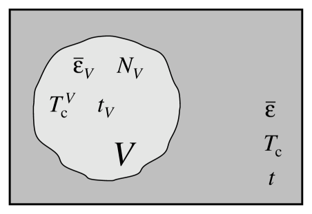
Figure 3: A volume $V$ within the system and the associated local quantities

Now comes the crucial intuitive step. Clearly, the critical temperature $T_{\mathrm{c}}$ depends on the average coupling constant $\bar{\varepsilon}=\varepsilon_{0}$. Thus, due to the fluctuations in the couplings $\varepsilon_{j,k}$, the system may locally, i.e., within a volume $V$, correspond to a different ‘local critical temperature’ $T_{\mathrm{c}}^{V}$ that, for sufficiently small disorder, may be expected to depend linearly on the local average coupling $T_{\mathrm{c}}^{V}\sim\bar{\varepsilon}_{V}$. One may think of $T_{\mathrm{c}}^{V}$ as the critical temperature of a system that essentially looks the same in any ball of volume $V$. Correspondingly, we may define a ‘local reduced temperature’ $t_{V}$.

If the disorder is irrelevant for the critical behaviour, the shift in the local reduced temperature $\udelta t=t_{V}-t$ has to vanish at criticality, i.e., $\udelta t\rightarrow 0$ as $t\rightarrow 0$. The relevance criterion now follows from this consistency requirement by using scaling relations involving the critical exponent $\nu$, which in the case of irrelevant disorder should coincide with the exponent $\nu_{0}$ of the pure system. The argument proceeds as follows. The volume $V$ of spins that are correlated is of the order $V\sim\xi^{d}$, where $\xi$ denotes the correlation length, and $d$ the dimension of the system. Then, from (19) and our assumption $T_{\mathrm{c}}^{V}\sim\bar{\varepsilon}_{V}$, we deduce

$$\udelta t\sim\xi^{-d(1-\omega)}\sim|t|^{\nu d(1-\omega)}\;,$$ (20)

where $\nu$ is the correlation exponent of the disordered system. In the irrelevant scenario $\nu=\nu_{0}$, this yields

$$\udelta t/t\sim|t|^{-\Phi}\qquad\mbox{with $\Phi=1-d\nu_{0}(1-\omega)$}\;.$$ (21)

Consequently, the disorder is irrelevant if the crossover exponent $\Phi<0$.

We can summarize the Harris-Luck relevance criterion as follows Har ; Luck ; Her . A modulation in $d_{\mathrm{m}}\leq d$ space dimensions of a ferromagnetic $d$-dimensional Ising model with correlation exponent $\nu_{0}$ is relevant for $\omega>\omega_{\mathrm{c}}$, marginal for $\omega=\omega_{\mathrm{c}}$, and irrelevant for $\omega<\omega_{\mathrm{c}}$, where

$$\omega_{\mathrm{c}}=1-\frac{1}{d_{\mathrm{m}}\nu_{0}}$$ (22)

and $\omega$ denotes the fluctuation exponent (19).

For the two-dimensional Ising model, we have $\nu_{0}=1$. Thus, for a model with layered disorder, i.e., $d_{\mathrm{m}}=1$, we obtain $\omega_{\mathrm{c}}=0$. In this case, any divergent fluctuation is relevant. For planar disorder, i.e., $d_{\mathrm{m}}=2$, the marginal value is $\omega_{\mathrm{c}}=1/2$. Thus, for randomly distributed couplings, which correspond to $\omega=1/2$, one is precisely in the marginal situation where the criterion does not give a definite prediction. Generally, one might expect to find logarithmic corrections to scaling in the marginal case, and this is indeed the case in the two-dimensional random-bond Ising model DD ; Shalaev ; Shankar ; Ludwig .

In the original formulation by Harris, the criterion was expressed in terms of the specific heat exponent $\alpha$ in place of the correlation exponent $\nu$. The two exponents are related by the hyperscaling relation $d\nu=2-\alpha$ Bax , which holds for the two-dimensional Ising model, which again corresponds to the marginal case $\alpha=0$ in the case of random disorder Har .

4 Random Ising Models

Traditionally, randomness was introduced into Ising models to describe magnetic behaviour of alloys where some magnetic atoms were replaced by non-magnetic atoms. Therefore, such models are termed dilute Ising models, and, in the simplest case, just correspond to a regular Ising model where some spins, or some bonds, have been removed, see the reviews Stinch ; Selke ; SST . Clearly, there is some relation to percolation RAR , because one at least needs infinite clusters in order to support a phase transition. Somewhat more general are random-bond Ising models, where the coupling constants are chosen randomly, often from a bimodal distribution.

In these systems, the disorder is regarded as ‘frozen’ or ‘quenched’, which means that it is static. Therefore, one has to average on the free energy on the possible realizations, which is extremely difficult Engel . Nevertheless, some analytical results have been obtained. As shown above, we expect the two-dimensional system to be marginal with respect to random disorder. Using the replica method, Dotsenko and Dotsenko DD found a double logarithmic singularity in the specific heat

$$c(t)\sim\ln[1+g\ln(1/|t|)]\;,$$ (23)

in place of the pure Ising behaviour (13), and

$$m(t)\sim\exp\{-a[\ln\ln(1/|t|)]^{2}/2\}\;,\qquad\chi(t)\sim t^{-2}\exp\{-a[\ln\ln(1/|t|)]^{2}\}\;,$$ (24)

corresponding to critical exponents $\beta=0$ and $\gamma=2$, which differ from the pure Ising values. However, by means of bosonization techniques and conformal field theory, Shalaev, Shankar, and Ludwig Shalaev ; Shankar ; Ludwig arrived at different results

$$m(t)\sim t^{1/8}(\ln|t|)^{-1/16}\;,\qquad\chi(t)\sim t^{-7/4}(\ln|t|)^{7/8}\;,$$ (25)

for the magnetization and the susceptibility, while the result for the specific heat coincides with (23). Here, the critical exponents keep their pure Ising values $\beta=1/8$ and $\gamma=7/4$, but logarithmic corrections show up. Due to the slow variation of the logarithm, it turns out to be very difficult to obtain reliable results from numerical calculations, because the logarithmic dependence on the reduced temperature translated to a logarithmic dependence on the system size, and it is hopeless to distinguish a simple logarithmic from a double logarithmic from finite-size calculations. Still, the majority of the numerous finite-size scaling studies based on Monte Carlo simulations or transfer matrix calculations favour the latter result (25), see Stinch ; Selke ; SST and references therein, which was also substantiated by a recent series expansion investigation RAJ .

The correlation exponent of the three-dimensional pure Ising model $\nu\approx 0.63$, thus $\alpha>0$, and disorder should be relevant in that case. However, a recent result indicates that for purely topological disorder introduced by considering an Ising model on a three-dimensional random graph the critical behaviour stays the same as for the regular cubic lattice JV .

In recent years, there has been an increasing activity in the mathematical literature on stochastic Ising model, see, e.g., New ; BP ; GHM , leading to a number of rather general rigorous results. For instance, for the random-field Ising model, it can be shown rigorously that for dimensions $d\leq 2$ there exists a unique Gibbs state, thus there is no phase transition in the two-dimensional random-field model, whereas there is a phase transition in $d\geq 3$. For ferromagnetic random-bond Ising models on certain periodic planar graphs, it was proven that at most two extremal Gibbs states exist, so there are no more than two phases, see GH and references therein.

5 Aperiodic Ising Models

In the remainder of this article, we shall concentrate on the case of aperiodically ordered Ising models GB . To this end, we need to introduce aperiodic sequences and tilings, see B for a recent review of the mathematical aspects. In the theoretical description of quasicrystalline structures SSH , aperiodic tilings constitute the the analogues of periodic lattices in conventional crystallography. For the sake of space, we cannot go into much detail here. The interested reader is referred to the Mathematica wolfram program packages accompanying this article, which give an insight into the construction and properties of one- and two-dimensional aperiodic tilings. The different methods employed and the corresponding Mathematica routines were described in detail in GS .

5.1 Aperiodic Tilings on the Computer

Aperiodic sequences are commonly constructed by means of substitution rules. As examples, consider an alphabet of two letters $a$ and $b$ and rules

$$\varrho^{(k)}:\;\;\begin{array}[]{lcl}a&\rightarrow&ab\\ b&\rightarrow&a^{k}\end{array}\qquad(k=1,2,\ldots)$$ (26)

that replace the single letters $a$ and $b$ by words $w_{a}^{(k)}=ab$ and $w_{b}^{(k)}=a^{k}$, the word consisting of $k$ letters $a$, in the two-letter alphabet $\{a,b\}$. We restrict ourselves to primitive substitutions, i.e., after a finite number of iterations the words obtained from the basic letters should contain all letters. Corresponding semi-infinite substitution sequences $w_{\infty}^{(k)}$ are then obtained by as fixed points of the substitution rules by an iterated application $w_{n}^{(k)}=\varrho^{(k)}(w_{n-1}^{(k)})$ of the rules (26) on some initial word, say $w_{0}^{(k)}=a$. The substitution rules (26) yield some prominent examples of aperiodic sequences, for instance the Fibonacci sequence $abaababa\ldots$ for $k=1$, the so-called periodic-doubling sequence $abaaabab\ldots$ for $k=2$, and a sequence known as the binary non-Pisot sequence $abaaaababab\ldots$ for $k=3$.

Many properties of the substitution sequences can conveniently be calculated form the associated substitution matrices

$$M^{(k)}=\left(\begin{array}[]{@{\,}r@{\;\;}r@{\,}}1&k\\ 1&0\end{array}\right)\;,\qquad\lambda_{\pm}^{(k)}=\frac{1\pm\sqrt{4k+1}}{2}\;,$$ (27)

whose elements just count the number of letters $a$ and $b$ in their substitutes $w_{a}^{(k)}$ and $w_{b}^{(k)}$, respectively. The largest eigenvalue $\lambda_{+}^{(k)}$ of $M^{(k)}$ determines the asymptotic growth of the sequence in one iteration step, while the entries of the corresponding eigenvector, suitably normalized, determine the frequencies $p_{a}=1-p_{b}=1-2/(3+\sqrt{4k+1})$ of the letters $a$ and $b$ in $w_{\infty}^{(k)}$. The second eigenvalue measures the fluctuations of the letter frequencies

$$g^{(k)}(N)=\#_{a}[{w^{(k)}_{\infty}}_{|N}]-p_{a}N\;,\qquad h^{(k)}(N)=\max_{M\leq N}\left|g^{(k)}(M)\right|\sim N^{\omega^{(k)}}\;,$$ (28)

where $\#_{a}[{w^{(k)}_{\infty}}_{|N}]$ denotes the number of letters $a$ in the first $N$ letters of the limit word $w^{(k)}_{\infty}$. Thus, $g^{(k)}(N)$ measures te deviation from the mean $p_{a}N$, and we use the maximal deviation $h^{(k)}(N)$ to define the fluctuation exponent $\omega^{(k)}$ which enters the Harris-Luck criterion, compare (19). It is given by

$$\omega^{(k)}=\frac{\ln|\lambda_{-}^{(k)}|}{\ln\lambda_{+}^{(k)}}\;;\qquad\omega^{(1)}=-1\;,\quad\omega^{(2)}=0\;,\quad\omega^{(3)}\approx 0.317>0\;;$$ (29)

and thus, according to the Harris-Luck criterion, a layered aperiodicity introduced into the Ising model according to these substitution rules is irrelevant for $k=1$, marginal for $k=2$, and relevant for $k=3$. So, contrary to what one might have expected, deterministic substitution sequences, albeit being non-random, actually provide examples for all interesting classes of ‘disorder’.

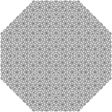
Figure 4: Eightfold patch of the Ammann-Beenker tiling

The Mathematica program FibonacciChain.m that is included in the program package offers the reader the opportunity to gain experience with substitution sequences and their properties. In addition, it also shows how quasiperiodic examples, such as the Fibonacci chain, can be derived from a projection of the two-dimensional square lattice. This approach, known as the cut-and-project method, can be generalized to higher dimensions to obtain quasiperiodic tilings (or in mathematical terminology, model sets B ) with interesting symmetry properties. Roughly, a certain part of the high-dimensional periodic lattice is projected onto a suitably chosen subspace. As an example, Fig. 4 shows a central patch of an eightfold symmetric planar tiling obtained from projection of the hypercubic lattice $\mathbb{Z}^{4}$. The tiling consists of squares and rhombi and is known as the octagonal or the Ammann-Beenker tiling ABS . In addition, this geometric structure also admits an inflation/deflation symmetry that is analogous to the substitution rule for the one-dimensional sequences. It consists of a dissection of the two basic tiles into copies of itself, such that the resulting tiling is, apart from an overall scaling, invariant under the procedure.

Both approaches are used in the Mathematica program OctagonalTiling.m GS . The remaining programs ChairTiling.m and SphinxTiling.m deal with two further planar examples of inflation tilings, while GridMethod.m introduces a variant of the cut-and-project scheme GS . The package PenrosePuzzle.m employs yet another method to construct the most famous among the zoo of quasiperiodic tilings, Penrose’s tiling of the plane. Here, the two basic rhombi are marked by certain arrow decorations on their edges, and it is the task to fill the entire plane with tiles without holes or overlaps, and without violating the matching rules that require that arrow decorations on adjacent edges have to match. The reader should be warned that this, albeit seemingly simplest, puzzle method is not suited to construct a large patch of the tiling because the matching rules do not uniquely specify how to add tiles, and, in particular, do not prevent implicit mistakes which will only be revealed when, at a certain stage, no further legal additions of tiles are possible. But, if you indeed managed to fill the entire plans without violating the rules, then the resulting tiling is a Penrose tiling with all the other ‘magic’ properties such as an inflation/deflation symmetry.

5.2 Ising Models on Planar Aperiodic Graphs

In what follows, we shall consider planar Ising models defined on quasiperiodic graphs, and, subsequently, Ising quantum chains with coupling constants varying according to substitution sequences. The latter correspond to two-dimensional classical Ising models with a layered aperiodicity, thus $d_{\mathrm{m}}=1$ in Harris-Luck criterion, and $\omega_{\mathrm{c}}=0$.

It may be surprising, but it is indeed possible to construct planar aperiodic Ising models that are exactly solvable BGB ; GB in the sense of commuting transfer matrices Bax . For such systems, the coupling constants have to be chosen in a particular way to ensure the integrability BGB . As a consequence, they have the rather unusual property that the free energy does not depend on the actual distribution of coupling constant, but only on the frequencies of the various couplings. Another evidence of the particular arrangement is the fact that the local magnetization, i.e., the expectation value of a spin at a certain site, does not depend on the site, but is uniform on the entire system. Therefore, the geometric arrangement of couplings does not play a rôle, and the critical behaviour is always the same as in the pure system. Nevertheless, these models are interesting because they provide counter-examples to the Harris-Luck criterion, because the previous statement also holds for arrangements with strong fluctuations that should have been relevant. However, the solvable examples are certainly very special, and possess some hidden underlying symmetry; and one should expect that the criterion holds for any generic distribution of coupling constants. Still, it reveals the limited predictive power of such criteria.

Ising models on quasiperiodic graphs, in particular the Penrose tiling, have been thoroughly investigated by means of Monte Carlo simulations and by approximative renormalization group treatments, see GB and the literature cited therein. Usually, the coupling is taken uniform along the bonds of the graph, so the fluctuations arise solely from the locally differing coordination numbers. This type of planar aperiodicity is irrelevant according to the Harris-Luck criterion, because the fluctuations for quasiperiodic cut-and-project sets, such as the Penrose tiling or the Ammann-Beenker tiling shown in Fig. 4, are small. Essentially, this is due to the fact that the quasiperiodic tiling is the projection of a slab of a periodic lattice, and thus, despite being aperiodic, these tilings show a pronounced regularity. The numerical results unanimously corroborate the prediction of the Harris-Luck criterion, and, undoubtedly, these models belong to the same universality class as the square-lattice Ising model.

Apart from these predominantly numerical approaches, also some analytical techniques have been employed. This concerns, for instance, high- and low-temperature expansions Domb that can be adapted to quasiperiodic systems. For the Penrose and the Ammann-Beenker tiling, the high-temperature expansion of the relevant part $\tilde{f}$ of the free energy,

$$\tilde{f}=\sum_{n=2}^{\infty}\,g_{2n}\,w^{2n}\;,\qquad w=\tanh(\beta J)\;,$$ (30)

where $J$ denotes the coupling constant, has recently been calculated to the 18th order in $w$ RGS1 . The coefficients $g_{2n}$ can be calculated from the frequencies of certain graphs of circumference $2n$ in the tiling, which, for cut-and-project sets, can be calculated explicitly. Furthermore, each graph carries a certain weight; these weights can be computed recursively. As an example, the expansion for the Ammann-Beenker tiling is given by

$$\textstyle w^{4}+\lambda w^{6}+(47\frac{1}{2}\!-\!17\lambda)w^{8}+(138\!-\!50\lambda)w^{10}+(803\frac{1}{3}\!-\!310\frac{1}{2}\lambda)w^{12}$$

$$\textstyle+(586\lambda\!-\!1220)w^{14}+(96\frac{3}{4}\!+\!295\frac{1}{2}\lambda)w^{16}+(46566\frac{1}{3}\lambda\!-\!108706)w^{18}+O(w^{20})$$

where $\lambda=1+\sqrt{2}$. This may be compared with the square-lattice result Domb

$$\textstyle w^{4}+2w^{6}+4\frac{1}{2}w^{8}+12w^{10}+37\frac{1}{3}w^{12}+130w^{14}+490\frac{1}{4}w^{16}+1958\frac{2}{3}w^{18}+O(w^{20})$$

where the coefficients are rational numbers. From the radius of convergence of the series, and the behaviour close to it, one can, in principle, derive the critical temperature and the thermal critical exponent. However, the information about the critical behaviour that one can extract from the expansion is rather poor, because, in contrast to the square-lattice case, the extrapolated values show extremely strong fluctuations RGS1 ; RGS2 , and much more terms would be necessary in order to give reliable estimates of the critical temperature and the critical exponents. But this is not feasible; a total of $244\,638$ different subgraphs of the Ammann-Beenker tiling contribute to the coefficient $g_{18}$, as compared with a mere $1975$ different graphs in the square-lattice case. A series analysis of other quantities such as the magnetic susceptibility may yield more stringent evidence, but this has not yet been calculated because the number of graphs that have to be considered is even larger.

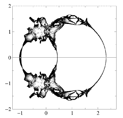
Figure 5: Part of partition function zeros in the complex variable $z=\exp(2J/k_{\mathrm{B}}T)$ for a periodic approximant of the Ammann-Beenker tiling with $41$ spins per unit cell

Another method that relies on the computation of the zeros of the partition function, in the complex temperature variable $z=\exp(2J/k_{\mathrm{B}}T)$. The set of zeros accumulates on certain curves or areas in the complex plane that separate different analytic domains, hence different phases of the system. Thus, a zero on the real positive axis will correspond to a phase transition point of the model, and the zeros close to this point contain information about the critical exponents. For periodic approximants of aperiodic tilings with rather large unit cells, the zero patterns can be calculated explicitly RGS2 . The result for an approximant of the Ammann-Beenker tiling, shown in Fig. 5, is rather involved, whereas for the square lattice case, the zeros are restricted to two circles with radius $\sqrt{2}$, centred at $z=\pm 1$. The two intersections of the zero pattern with the real axis correspond to the ferromagnetic ($J>0$) and antiferromagnetic ($J<0$) critical point, respectively, which are related to each other because the tiling is bipartite. The corresponding estimates of the critical temperature are given in Table 1. Clearly, this method allows a very precise determination of the critical temperature, in good agreement with, less accurate, Monte Carlo results Oli .

Table 1: Critical temperatures $w_{\mathrm{c}}=\tanh(J/K_{\mathrm{B}}T_{\mathrm{c}})$ for periodic approximants of the Ammann-Beenker tiling, and estimated value for the aperiodic tiling

$m$	$N$	$w_{c}$
$1$	$7$	$0.396\,850\,570$
$2$	$41$	$0.396\,003\,524$
$3$	$239$	$0.395\,985\,346$
$4$	$1393$	$0.395\,984\,811$
$5$	$8119$	$0.395\,984\,795$
$6$	$47321$	$0.395\,984\,795$
$\infty$	$\infty$	$0.395\,984\,79(1)$

5.3 Aperiodic Ising Quantum Chains

We now turn our attention to the case of one-dimensional aperiodicity and consider Ising quantum chains with aperiodically modulated coupling constants GB

$$H=-\frac{1}{2}\left(\sum\limits_{j=1}^{N}\varepsilon_{j}\,\sigma^{x}_{j}\sigma^{x}_{j+1}+\sum\limits_{j=1}^{N}h_{j}\sigma^{z}_{j}\right)\;,$$ (31)

where, in contrast to (14), the couplings $\varepsilon_{j}\in\{\varepsilon_{a},\varepsilon_{b}\}$ and the transversal fields $h_{j}\in\{h_{a},h_{b}\}$ are chosen according to the $j$th letter of an aperiodic substitution sequence.

Such models can be treated by an exact real-space renormalization approach, exploiting the recursive structure that is already inherent in the substitution sequence IT ; ITKS ; HGB ; HG ; Her . The basic idea behind this approach is that a renormalization step reverses a substitution step, i.e., the Hamiltonian is transformed into a Hamiltonian at the previous substitution level, which just differs from the original Hamiltonian by renormalized values of the parameters. The renormalization transformation then becomes a mapping in the finite-dimensional parameter space of the Hamiltonian, and the renormalization transformation is exact because no additional parameters have to be introduced. This is very interesting because it provides one of the few examples with an exact renormalization transformation for a non-trivial model, keeping in mind that the usual decimation approach does not work even for the square-lattice Ising model. Furthermore, it works for arbitrary substitution sequences HGB ; Her , not just for our examples (26), and can even be applied to the case of random substitutions Her . This encompasses a large class of models with different fluctuations in the couplings and, consequently, different physical behaviour. For the sake of space, we cannot go into detail here, but just briefly sketch the calculation.

The first step consists of a mapping of the Hamiltonian (31) onto a model of free fermions,

$$H=\sum_{j=1}^{N}\Lambda_{j}\,\eta_{j}^{\dagger}\eta_{j}\>+\>C\;,\qquad\{\eta_{j},\eta_{\ell}\}=\{\eta_{j}^{\dagger},\eta_{\ell}^{\dagger}\}=0\;,\quad\{\eta_{j}^{\dagger},\eta_{\ell}\}=\delta_{j,\ell}\;,$$ (32)

by means of a Jordan-Wigner transformation LSM . In this way, the task of computing the spectrum of (31) is reduced from the diagonalization of a $2^{N}\times 2^{N}$ matrix to that of the $2N\times 2N$ eigenvalue problem

$$\left(\begin{array}[]{@{}cccccccc@{}}0&h_{1}&0&0&0&\cdots&0&\varepsilon_{N}\\ h_{1}&0&\varepsilon_{1}&0&0&\cdots&0&0\\ 0&\varepsilon_{1}&0&h_{2}&0&\cdots&0&0\\ 0&0&h_{2}&0&\varepsilon_{2}&\cdots&0&0\\ \vdots&\vdots&\ddots&\ddots&\ddots&\ddots&&\vdots\\ 0&0&\cdots&0&\makebox[0.0pt]{$h_{\scriptscriptstyle N-1}$}&0&\makebox[0.0pt]{$\varepsilon_{\scriptscriptstyle N-1}$}&0\\ 0&0&\cdots&0&0&\makebox[0.0pt]{$\varepsilon_{\scriptscriptstyle N-1}$}&0&h_{N}\\ \varepsilon_{N}&0&\cdots&0&0&0&h_{N}&0\end{array}\right)\left(\begin{array}[]{l@{}}\Phi_{1}\\ \Psi_{1}\\ \Phi_{2}\\ \Psi_{2}\\ \;\vdots\\ \Psi_{\scriptscriptstyle N-1}\\ \Phi_{N}\\ \Psi_{N}\\ \end{array}\right)=\Lambda\left(\begin{array}[]{l@{}}\Phi_{1}\\ \Psi_{1}\\ \Phi_{2}\\ \Psi_{2}\\ \;\vdots\\ \Psi_{\scriptscriptstyle N-1}\\ \Phi_{N}\\ \Psi_{N}\\ \end{array}\right)$$ (33)

whose $N$ positive solutions $0\leq\Lambda_{1}\leq\Lambda_{2}\leq\ldots\leq\Lambda_{N}$ determine the entire spectrum of the Hamiltonian (31). The quantum phase transition appears when the lowest excitation energy tends to zero, $\Lambda_{1}\rightarrow 0$, in the thermodynamic limit $N\rightarrow\infty$, so we can concentrate on the low-energy behaviour.

The renormalization equations can now be derived by exploiting the recursive structure of the sequence, effectively combining those sites that belong to a single letter at the previous stage of the substitution rule. This results in a mapping in parameter space, which can be expanded in powers of $\Lambda$ at the fixed point $\Lambda=0$, which corresponds to the critical point given by the condition

$$1=\lim_{N\rightarrow\infty}\left|\frac{\varepsilon_{1}}{h_{1}}\frac{\varepsilon_{2}}{h_{2}}\ldots\frac{\varepsilon_{N}}{h_{N}}\right|^{\frac{1}{N}}=\left|\frac{\varepsilon_{a}}{h_{a}}\right|^{p_{a}}\left|\frac{\varepsilon_{b}}{h_{b}}\right|^{p_{b}}$$ (34)

where the last equality applies to the two-letter case discussed above. It can be parametrized as $|\varepsilon_{a}/h_{a}|=r^{-p_{b}}$ and $|\varepsilon_{b}/h_{b}|=r^{p_{a}}$ with $r\in\mathbb{R}^{+}$. The mapping determines the finite-size scaling of the smallest excitation energy $\Lambda_{1}$, and thus the critical behaviour. In complete accordance with the Harris-Luck criterion, we find that $\Lambda_{1}\sim v(r)N^{-1}$ for irrelevant aperiodicity, as in the periodic case. For marginal aperiodicity, we observe $\Lambda_{1}\sim N^{-z(r)}$ with a coupling-dependent non-universal exponent $z(r)$, corresponding to an anisotropic scaling of the correlation length with different exponents $\nu_{\parallel}$ and $\nu_{\perp}$. For relevant aperiodicity, we find that the lowest excitation energy vanishes exponentially, $\Lambda_{1}\sim\exp[-\Delta(r)N^{\omega}]$, where $\omega$ is the fluctuation exponent (19). In fact, we can calculate also the non-universal coupling-dependent terms. For our examples at hand, this yields $v(r)=2\ln(r)/(r-1/r)$ for the Fibonacci chain $k=1$ (26), the exponent $z(r)=\ln(r^{1/3}+r^{-1/3})/\ln(2)$ for the period-doubling sequence $k=2$ (26), and the coefficient $\Delta(r)=\sqrt{2\sqrt{13}-7}|\ln(r)|$ for the binary non-Pisot sequence $k=3$ (26). This renormalization approach can also be applied to obtain information about the eigenvector in (33), thus determining the behaviour of the surface magnetization in an open quantum chain HG . Furthermore, other free-fermion models such as the XY chain can also be treated Her ; Joachim .

6 Summary and Conclusions

The article gives a brief overview on recent results for aperiodic Ising models. According to the personal taste and scientific experience of the author, aperiodically ordered Ising models received most attention, while random Ising models were only discussed from a qualitative perspective. It is shown that heuristic scaling arguments like the Harris-Luck criterion can provide a rather powerful tool that, in most cases, correctly predict whether or not a certain disorder will affect the critical behaviour. Still, behind the scene are a number of tacit assumptions, and there exist at least exceptional systems which defy the relevance criterion, as shown by an exactly solvable example.

It is quite a difficult task to treat randomly disordered or aperiodically ordered planar Ising models analytically, and rather sophisticated techniques have been employed. However, it turns out that the Ising quantum chain with coupling constants modulated according to substitution sequences can be solved by an exact real-space renormalization approach, thus proving the validity of the Harris-Luck criterion for this entire class of models and, in addition, providing information about the non-universal coefficient that enter the scaling behaviour.

References

- (1) R. Balian: From Microphysics to Macrophysics, vol. I (Springer, Berlin 1991)
- (2) D. Frenkel: Physica A 263, 26 (1999)
- (3) R.J. Baxter: Exactly Solved Models in Statistical Mechanics (Academic Press, London 1982)
- (4) W. Lenz: Physikalische Zeitschrift 21, 613 (1920)
- (5) E. Ising: Zeitschrift für Physik 31, 253 (1925)
- (6) L. Onsager: Phys. Rev. 65, 117 (1944)
- (7) J.-B. Suck, M. Schreiber, P. Häussler (eds.): Quasicrystals (Springer, Berlin 2001) to appear
- (8) L.P. Kadanoff: ‘Scaling, universality and operator algebras’. In: Phase Transitions and Critical Phenomena vol. 5a, ed. by C. Domb, J.L. Lebowitz (Academic Press, London 1976) pp. 1–34
- (9) K. Binder (this volume)
- (10) R. Römer (this volume)
- (11) F. Schwabl (this volume)
- (12) T. Vojta (this volume)
- (13) J.L. Cardy: Scaling and Renormalization in Statistical Physics (Cambridge University Press, Cambridge 1996)
- (14) P. DiFrancesco, P. Mathieu, D. Sénéchal: Conformal Field Theory (Springer, New York 1997)
- (15) B.M. McCoy, T.T. Wu: The two-dimensional Ising Model (Harvard University Press, Cambridge, Massachusetts, 1973)
- (16) H.-O. Georgii: Gibbs Measures and Phase Transitions (de Gruyter, Berlin 1988)
- (17) S. Kobe: J. Stat. Phys. 88, 991 (1997); Phys. Blätter 54, 917 (1998)
- (18) U. Grimm, M. Baake: ‘Aperiodic Ising models’. In: The Mathematics of Long-Range Aperiodic Order, ed. by R.V. Moody (Kluwer, Dordrecht 1997) pp. 199-237
- (19) R. Peierls: Proc. Cambridge Philos. Soc. 32, 477 (1936)
- (20) R.S. Ellis: Entropy, Large Deviations, and Statistical Mechanics (Springer, New York 1985)
- (21) H.A. Kramers, G.H. Wannier: Phys. Rev. 60, 252 (1941)
- (22) C.N. Yang: Phys. Rev. 85, 808 (1952)
- (23) R.B. Stinchcombe: J. Phys. C 6, 2459 (1973)
- (24) E. Lieb, T. Schultz, D. Mattis: Ann. Phys. (NY) 16, 407 (1961)
- (25) J.B. Kogut: Rev. Mod. Phys. 51, 659 (1979)
- (26) C. Chatelain, P.E. Berche, B. Berche: Eur. Phys. J. B 7, 439 (1999)
- (27) J. Hermisson: Aperiodische Ordnung und Magnetische Phasenübergänge (Shaker, Aachen 1999)
- (28) A.B. Harris: J. Phys. C: Solid State Phys. 7, 1671 (1974)
- (29) J.M. Luck: J. Stat. Phys. 72, 417 (1993); Europhys. Lett. 24, 359 (1993)
- (30) A. Engel (this volume)
- (31) R.B. Stinchcombe: ‘Dilute magnetism’. In: Phase Transitions and Critical Phenomena vol. 7, ed. by C. Domb, J.L. Lebowitz (Academic Press, London 1983) pp. 151–280
- (32) W. Selke, ‘Monte Carlo simulations of dilute Ising models’. In: Computer Simulation Studies in Condensed Matter Physics IV, ed. by D.P. Landau, K.K. Mon, H.-B. Schüttler (Springer, Berlin 1993) pp. 18–27
- (33) W. Selke, L.N. Shchur, A.L. Talapov: ‘Monte Carlo simulations of dilute Ising models’. In: Annual Reviews of Computational Physics I, ed. by D. Stauffer (World Scientific, Singapore 1994) pp. 17–54
- (34) Vik. S. Dotsenko, Vl. S. Dotsenko: Adv. Phys. 32, 129 (1983)
- (35) B.N. Shalaev: Sov. Phys. Solid State 26, 1811 (1984); Phys. Rep. 237, 129 (194)
- (36) R. Shankar: Phys. Rev. Lett. 58, 2466 (1987); 61, 2390 (1988)
- (37) A.W.W. Ludwig: Phys. Rev. Lett. 61, 2388 (1988); Nucl. Phys. B 330, 639 (1990)
- (38) A. Roder, J. Adler, W. Janke: Phys. Rev. Lett. 80, 4697 (1998)
- (39) W. Janke, R. Villanova, ‘Ising spins on 3D random lattices’. In: Computer Simulation Studies in Condensed Matter Physics XI, ed. by D.P. Landau, H.-B. Schüttler (Springer, Berlin 1999) pp. 22–26
- (40) C.M. Newman: Topics in Disordered Systems (Birkhäuser, Basel 1997)
- (41) A. Bovier, P. Picco (eds.): Mathematical Aspects of Spin Glasses and Neural Networks, Progress in Probability 41 (Birkhäuser, Boston 1998)
- (42) H.-O. Georgii, O. Häggström, C. Maes: ‘The random geometry of equilibrium phases’. Preprint math.PR/9905031, to appear in: Phase Transitions and Critical Phenomena, ed. by C. Domb, J.L. Lebowitz (Academic Press, London)
- (43) H.-O. Georgii, Y. Higuchi: J. Math. Phys. 41, 1153 (2000)
- (44) M. Baake: ‘A guide to mathematical quasicrystals’. Preprint math-ph/9901014, to appear in SSH
- (45) S. Wolfram: Mathematica: A System for Doing Mathematics by Computer, 2nd ed. (Addison-Wesley, Reading, Massachusetts 1991)
- (46) U. Grimm, M. Schreiber: ‘Aperiodic tilings on the computer’. Preprint cond-mat/9903010, to appear in SSH
- (47) R. Ammann, B. Grünbaum, G. Shephard: Discrete Comput. Geom. 8, 1 (1992)
- (48) M. Baake, U. Grimm, R.J. Baxter: Int. J. Mod. Phys. B 8 3579 (1994)
- (49) C. Domb: ‘Ising model’. in: Phase Transitions and Critical Phenomena vol. 3 ed. by C. Domb, M.S. Green (Academic Press, London 1974) pp. 357–458
- (50) P. Repetowicz, U. Grimm, M. Schreiber: J. Phys. A: Math. Gen. 32, 4397 (1999)
- (51) P. Repetowicz, U. Grimm, M. Schreiber: ‘Planar quasiperiodic Ising models’. Preprint cond-mat/9908088
- (52) O. Redner, M. Baake: J. Phys. A: Math. Gen. 33, 3097 (2000)
- (53) F. Iglói, L. Turban: Phys. Rev. Lett. 77, 1206 (1996)
- (54) F. Iglói, L. Turban, D. Karevski, F. Szalma: Phys. Rev. B 56, 11031 (1997)
- (55) J. Hermisson, U. Grimm, M. Baake: J. Phys. A: Math. Gen. 30, 7315 (1997)
- (56) J. Hermisson, U. Grimm: Phys. Rev. B 57, R673 (1998)
- (57) J. Hermisson: J. Phys. A: Math. Gen. 33, 57 (2000)