Crystal structures and freezing of dipolar fluids

Abstract

We investigate the crystal structure of classical systems of spherical particles with an embedded point dipole at $T=0$. The ferroelectric ground state energy is calculated using generalizations of the Ewald summation technique. Due to the reduced symmetry compared to the nonpolar case the crystals are never strictly cubic. For the Stockmayer (i.e., Lennard-Jones plus dipolar) interaction three phases are found upon increasing the dipole moment: hexagonal, body-centered orthorhombic, and body-centered tetragonal. An even richer phase diagram arises for dipolar soft spheres with a purely repulsive inverse power law potential $\sim r^{-n}$. A crossover between qualitatively different sequences of phases occurs near the exponent $n=12$. The results are applicable to electro- and magnetorheological fluids. In addition to the exact ground state analysis we study freezing of the Stockmayer fluid by density-functional theory.

I Introduction

The last years have seen a revival of interest in simple dipolar fluids, which consist of spherical particles with embedded point dipoles, triggered by two unexpected observations: At high interaction strengths and high densities a liquid phase with long-range ferroelectric orientational order but without any positional order occurs [1]; at low densities the particles form a gas of chains behaving like living polymers [2]. The latter effect was suggested as an explanation for the apparent absence of gas-liquid condensation in dipolar hard spheres [3], but this subject is still under discussion [4]. Both phenomena have first been detected in computer simulations [5, 6, 7, 8, 9], followed by theoretical work [10, 11, 12, 13, 14]. This discussion applies to electric and magnetic dipoles in complete analogy; in the following we will use the electric language.

Knowledge about the solid phase of these systems is necessary in order to know under which circumstances formation of the ferroelectric liquid is preempted by freezing. This question has been tackled theoretically within two different versions of density-functional theory. Groh and Dietrich [15] found a stable ferroelectric liquid for the Stockmayer (i.e., dipolar Lennard-Jones) model if the dipole moment is high enough. Klapp and coworkers, however, found within their approach that the ferroelectric liquid is always metastable in comparison with the solid both for Stockmayer and dipolar hard sphere fluids [16, 17]. But in a recent study they demonstrated that their result depends sensitively on the applied approximations [18]. The only solid structures considered in these papers [15, 16, 17, 18] are face-centered cubic (fcc), which is the known crystal structure in the non-polar limit, and body-centered tetragonal (bct) with the special axis ratio $c/a=\sqrt{2/3}$, which had been determined before as the ground state of dipolar hard spheres [19] and has also been observed in simulations [20] and in experiments [21, 22] with electrorheological fluids, i.e., suspensions of polarizable colloidal particles.

In a recent simulation Gao and Zeng [23] confirmed the occurrence of a stable ferroelectric liquid phase for the Stockmayer model and, in addition, determined for the first time portions of the phase boundaries between isotropic and ferroelectric liquid and between ferroelectric liquid and solid. Although these results support the basic conclusion in Ref. [15] they found that the stable solid phase of the Stockmayer model is body-centered orthorhombic (bco) and additionally observed a metastable distorted hexagonal structure, possibilities that have not been taken into account in the theoretical work [15, 16, 17, 18] so far. Both bco and bct as well as an fcc crytal with helically varying polarization direction have been reported before in simulations of dipolar hard spheres [24], but the thermodynamically stable state could not be determined. Certain structures may be suppressed in simulations due to the periodic boundary conditions if the cell shape is not flexible enough.

A simple heurestic argument why a cubic structure is not expected runs as follows. All these crystals are ferroelectric and hence have less symmetry than in the nonpolar case; the point symmetries can only be reflections at planes that contain the polarization axis and rotations around this axis. Therefore if, e.g., in a cubic crystal a polarization in $[100]$ direction is switched on, the additional introduction of a contraction along this direction does not further reduce the remaining symmetry. Hence generically the crystal will have an axis ratio different from unity, i.e., it will be tetragonal. For polarization along the initial $[110]$ and $[111]$ directions the same reasoning leads to orthorhombic and trigonal crystals. Thus a ferroelectric solid can never be strictly cubic, in contrast to the assumptions made in the density-functional work described above and in similar work on the Heisenberg fluid [25].

Thus up to now it is quite unclear which crystal structure(s) actually are stable in these widely used dipolar model systems. As a first step to elucidate this region of their phase diagram in the present work we determine the ground state structure as a function of density, dipole strength, and softness of the isotropic interaction potential. Since in principle an infinite number of crystal structures exists, characterized by an increasing number of parameters with increasing number of particles in the basis, an exhaustive search for the ground state is not possible. However, we include a rather large class of candidate structures, comprising among others all reasonable simple Bravais lattices. A relatively complex phase behavior is found at $T=0$. There is reason to expect that the ground state results remain qualitatively valid at not too high temperatures and thus provide a valuable starting point for a more complete analysis of the full phase diagram.

In a recent work [26] ground state energies and ordering temperatures for ferroelectric and antiferroelectric arrangements of Ising dipoles on several lattices have been determined, but no attempt has been made to optimize the lattice structure. In this study also the presence of isotropic interactions was not taken into account.

In our analysis we always assume a spatially homogeneous polarization throughout the sample. In real ferroelectric materials domains will form due to the long range nature of the dipolar interaction [27]. The domain structure in the liquid ferroelectric phase for a cubic sample shape has been analyzed in detail in Ref. [28]. This more complicated situation is avoided in two cases: (i) a needle-shaped sample (infinite aspect ratio), implying a vanishing depolarization factor; (ii) cancelling of the induced surface charges by free charges which are present in a conducting surrounding medium or as impurities in the material itself.

After having reached a basically complete overview of the thermodynamically stable ground states in such systems, which is interesting in its own right, in a second step by using density-functional theory we return to the issue which solid phase the ferroelectric liquid phase the Stockmayer fluid forms upon freezing. This closes the aforementioned gap between the analysis of the solid phases as considered so far in the theoretical analyses [15, 16, 17, 18] and the observation of those types of solid structures as found in simulations [23]. It consolidates the theoretical prediction [15] that the Stockmayer fluid can exhibit a thermodynamically stable ferroelectric liquid phase, in accordance with the simulation results.

II Models and Methods

We study systems of spherical dipolar particles interacting via the dipolar potential

$$w_{dip}({\bf r})=\frac{-m^{2}r^{2}+3({\bf m}\cdot{\bf r})^{2}}{r^{5}}$$ (1)

where ${\bf r}$ is the interparticle vector and ${\bf m}$ the dipole moment, which is assumed to have the same orientation for all particles. In addition there is an isotropic interaction $w_{iso}$ which is taken as either the purely repulsive soft sphere (SS) potential

$$w_{SS}(r)=4\epsilon\left(\frac{\sigma}{r}\right)^{n}$$ (2)

or the Lennard-Jones (LJ) potential

$$w_{LJ}(r)=4\epsilon\left[\left(\frac{\sigma}{r}\right)^{12}-\left(\frac{\sigma}{r}\right)^{6}\right].$$ (3)

The parameters $\epsilon$ and $\sigma$ define the energy and length scales, respectively. The ground state properties only depend on the reduced dipole moment $m^{\ast}=(m^{2}/(\sigma^{3}\epsilon))^{1/2}$ and the reduced particle density $\rho^{\ast}=\sigma^{3}N/V$ of $N$ particles in the volume $V$. Since in the SS case only the combination $\epsilon\sigma^{n}$ enters the potential, the only independent thermodynamic parameter is $x={m^{\ast}}^{2}/{\rho^{\ast}}^{n/3-1}$. In the LJ case the ground state energy per particle $U$ has the form $U=\epsilon\hat{E}(\rho^{\ast},m^{\ast})$ whereas for the SS case one has $U=\epsilon{\rho^{\ast}}^{n/3}\bar{E}({m^{\ast}}^{2}/{\rho^{\ast}}^{n/3-1})$ where $\hat{E}$ and $\bar{E}$ are dimensionless scaling functions which contain all the structure dependence. For soft spheres the optimum structure remains the same as long as $x$ is kept constant because the prefactor ${\rho^{\ast}}^{n/3}$ is the same for all structures belonging to a given reduced density $\rho^{\ast}$. Furthermore one can show that also phase coexistence densities $\rho^{\ast}_{i}$ determined for one value of $m^{\ast}$ can be scaled to another dipole moment ${m^{\ast}}^{\prime}$ according to ${\rho^{\ast}}^{\prime}_{i}=(m^{\ast}/{m^{\ast}}^{\prime})^{6/(n-3)}\rho^{\ast}_{i}$, because $\partial(\rho^{\ast}U)/\partial\rho^{\ast}=\epsilon{\rho^{\ast}}^{n/3}E_{1}(x)$ with another scaling function $E_{1}$. Hence for the SS model without loss of generality we set $m^{\ast}=1$.

Explicitly the ground state energy per particle is

$$U=U_{dip}+U_{iso}=\frac{1}{2}{\sum_{{\bf R},{\boldsymbol{\tau}}}}^{\;\prime}\left[w_{dip}({\bf R}+{\boldsymbol{\tau}})+w_{iso}({\bf R}+{\boldsymbol{\tau}})\right]$$ (4)

where ${\bf R}$ runs over the $N_{l}$ lattice vectors of a Bravais lattice and ${\boldsymbol{\tau}}$ over the $M$ positions of the basis particles within one unit cell so that $N=N_{l}M$; the prime on the summation sign indicates that the term with ${\bf R}+{\boldsymbol{\tau}}=0$ must be omitted. Here we implicitly have replaced a double sum over the lattice sites by a single sum, assuming that the average energy per particle is equal to the energy of the particle at the origin. It is a non-trivial issue whether this assumption is justified for the long-ranged dipolar potential. In the appendix we show that it is correct for a homogeneous orientational configuration in an ellipsoidal sample shape, but not, e.g., for a parallelepiped. (But we recall that only under the conditions mentioned in the last but one paragraph of Sec. I the ground state has spatially homogeneous orientational order as assumed in Eq. (4).) Straightforward numerical calculation of these lattice sums is hampered by their slow convergence. Therefore generalizations of the Ewald technique are employed to transform the sums into a more rapidly converging form. The basic idea for evaluating adroitly a general sum $\sum_{\bf R}f({\bf R})$ is to write $f({\bf R})=h({\bf R})+g({\bf R})$ where $h({\bf R})$ decays rapidly in real space and the Fourier transform $\tilde{g}({\bf k})=\int d^{3}r\,e^{-i{\bf k}\cdot{\bf r}}g({\bf r})$ decays rapidly in reciprocal space [29]. The sum of $g$ is then evaluated in reciprocal space using the Poisson sum formula. For the inverse power sums with $f({\bf R})=R^{-n}$ one uses $h(R)=\Gamma(n/2,\nu^{2}R^{2})/(R^{n}\Gamma(n/2))$ where $\Gamma(a,x)$ is the incomplete Gamma function and obtains for a Bravais lattice [30, 29]

$$\sum_{{\bf R}\neq 0}\frac{1}{R^{n}}=\frac{1}{\Gamma(n/2)}\Big{[}\sum_{{\bf R}\neq 0}\frac{1}{R^{n}}\Gamma(n/2,\nu^{2}R^{2})+\frac{\pi^{3/2}}{V_{c}}\sum_{{\bf k}\neq 0}\left(\frac{k}{2}\right)^{n-3}\Gamma\left(\frac{3-n}{2},\frac{k^{2}}{4\nu^{2}}\right)\\ -\frac{2}{n}\nu^{n}+\frac{2}{n-3}\frac{\pi^{3/2}}{V_{c}}\nu^{n-3}\Big{]}.$$ (5)

Here ${\bf k}$ runs over the reciprocal lattice, $V_{c}$ is the volume of the unit cell and the last two contributions take into account the omissions of the terms $R=0$ and $k=0$. The parameter $\nu$ can be chosen arbitrarily and the independence of $\nu$ of the total sum provides a convenient check of the algorithm. In practice $\nu$ is chosen such that both sums converge approximately with the same rate. Typically a few hundred lattice vectors in real and reciprocal space are sufficient to obtain machine precision ($10^{-16}$). The straightforward generalization to $M$ particles in the basis leads to

$$U_{SS}^{(n)}=\frac{2\epsilon\sigma^{n}}{\Gamma(n/2)}\Big{[}{\sum_{{\bf R},{\boldsymbol{\tau}}}}^{\;\prime}\frac{\Gamma(n/2,\nu^{2}({\bf R}+{\boldsymbol{\tau}})^{2})}{|{\bf R}+{\boldsymbol{\tau}}|^{n}}+\frac{\pi^{3/2}}{V_{c}}\sum_{{\bf k}\neq 0}\sum_{\boldsymbol{\tau}}\cos({\bf k}\cdot{\boldsymbol{\tau}})\left(\frac{k}{2}\right)^{n-3}\Gamma(\frac{3-n}{2},\frac{k^{2}}{4\nu^{2}})\\ -\frac{2}{n}\nu^{n}+N\frac{2}{n-3}\frac{\pi^{3/2}}{V_{c}}\nu^{n-3}\Big{]}.$$ (6)

Clearly for the LJ case $U_{iso}=U_{SS}^{(12)}-U_{SS}^{(6)}$.

An analogous expression for the dipolar lattice sum can be obtained from the well-known result for the potential of a lattice of point charges [31]

$$U_{dip}=\frac{m^{2}}{2}\left[\sum_{{\bf R}\neq 0}\Phi_{\nu}({\bf R})+\frac{4\pi}{V_{c}}\sum_{{\bf k}\neq 0}\frac{k_{z}^{2}}{k^{2}}\exp(-\frac{k^{2}}{4\nu^{2}})-\frac{4\nu^{3}}{3\sqrt{\pi}}\right]$$ (7)

with

$$\Phi_{\nu}({\bf R})=\frac{2\nu}{\sqrt{\pi}R^{4}}(R^{2}-3R_{z}^{2}-2\nu^{2}R^{2}R_{z}^{2})e^{-\nu^{2}R^{2}}+\frac{R^{2}-3R_{z}^{2}}{R^{5}}\operatorname{erfc}(\nu R).$$ (8)

Due to the slow decay of $w_{dip}$ the dipolar sum is actually only conditionally convergent, i.e., the result is shape dependent. In the appendix we present the derivation of Eq. (7) and show that it corresponds to the case of a needle-shaped sample which is of interest here. The corresponding generalization to lattices with a basis reads

$$U_{dip}=\frac{m^{2}}{2}\left[{\sum_{{\bf R},{\boldsymbol{\tau}}}}^{\;\prime}\Phi_{\nu}({\bf R}+{\boldsymbol{\tau}})+\frac{4\pi}{V_{c}}\sum_{{\bf k}\neq 0}\sum_{\boldsymbol{\tau}}\cos({\bf k}\cdot{\boldsymbol{\tau}})\frac{k_{z}^{2}}{k^{2}}\exp(-\frac{k^{2}}{4\nu^{2}})-\frac{4\nu^{3}}{3\sqrt{\pi}}\right].$$ (9)

If the dipoles are not oriented along the $z$ axis of the lattice but have a general orientation $\hat{\bf m}$ the dipole sum has the form $\sum_{ij}\hat{m}_{i}T_{ij}\hat{m}_{j}$ with a symmetrical matrix $T_{ij}$ (see Eq. (1)). The optimum direction is then necessarily along one of the eigenvectors of $T$ which coincide with high symmetry lattice directions. Thus it suffices to consider only one or two possible orientations for each lattice.

The following crystal structures, displayed in Figs. 1 and 2, were included in the search for the minimum of the energy (except for trigonal lattices the polarization is always along the $c$ axis):

1. body-centered orthorhombic (bco) with axis lengths $a$, $b$, $c$; reduces to bct for $a=b$, to fcc polarized along $[110]$ for $b/a=c/a=1/\sqrt{2}$ (see Fig. 1), and to fcc polarized along $[001]$ for $b/a=1$, $c/a=\sqrt{2}$.

2. face-centered orthorhombic (fco); note that for the tetragonal case ($b=a$) face-centered and body-centered lattices are equivalent.

3. trigonal (trig): three equal axes with angle $\gamma$ between any pair of them, polarized along $[111]$; reduces to various cubic lattices polarized along $[111]$ for special values of $\gamma$.

4. hexagonal with axis lengths $a$, $c$ and a second basis particle at ${\boldsymbol{\tau}}=a/2(1,1/\sqrt{3},c/a)$ polarized along the $c$ axis (hexc); corresponds to hexagonal close packed (hcp) for $c/a=\sqrt{8/3}$.

5. an orthorhombic lattice with four basis particles at ${\boldsymbol{\tau}}_{0}=0$, ${\boldsymbol{\tau}}_{1}=(a/6,b/2,c/2)$, ${\boldsymbol{\tau}}_{2}=(a/2,0,c/2)$, and ${\boldsymbol{\tau}}_{3}=(2a/3,b/2,0)$ which can be viewed as a distorted hcp lattice with polarization in the $ab$-plane (hexab); this structure was observed in Ref. [23].

These possibilities have been chosen for the following reasons. The structures bco, hexc, and hexab are generated by slight distortions of the close packed fcc and hcp lattices which represent the ground state for $m=0$. The structures fco and trig are included, because they approach reasonable low density configurations in certain limits, which have been observed in electrorheological fluids [22]. For $\gamma\to 2\pi/3$ trig degenerates into a hexagonal array of dipolar chains, and for $c,b\gg a$ fco develops into a collection of parallel sheets. The only remaining Bravais lattices, monoclinic and triclinic, are improbable and also difficult to handle because of the larger number of free parameters. We tested a monoclinic variation of bco and always found that the energy is minimized for a right angle between the axes. Concerning more complex lattices it is difficult to define a reasonable parameter space without a physically motivated structure to start from.

III Results

A Stockmayer model at $T=0$

If one starts from the fcc structure of the nonpolar LJ system and introduces a dipole moment, all orientations of the polarization have the same energy, as long as the cubic symmetry is preserved. However, as discussed in the introduction, the crystal actually distorts towards bco, bct, or trig, depending on the direction of the polarization. The numerical findings indicate that the $[110]$ direction is selected, corresponding to a bco distortion as shown in Fig. 1. Intuitively this can be understood as a preference for the formation of chains along the polarization direction: $[110]$ points towards the nearest neighbors so that the particle distance along the chains is smallest in this case. Indeed, upon increasing the dipole moment the length of the $c$ axis decreases, reflecting the strong attractive interactions along the chains. Figure 3 displays the dependence of the bco axis ratios on the reduced dipole moment $m^{\ast}$. The result of Gao and Zeng [23] for $\rho^{\ast}=1.24$, $m^{\ast}=2.5$, and $T^{\ast}=k_{B}T/\epsilon=0.7$ denoted by the diamonds lies very close to the $T=0$ result. Obviously the ground state gives a good approximation to the equilibrium state at least up to half the triple temperature $T^{\ast}_{tr}\simeq 1.3$ [23]. The same authors also report a metastable hexab structure at $m^{\ast}=2.5$, $T^{\ast}=0.8$, and $\rho^{\ast}=1.146$ with the axis ratios $c/a=0.497$ and $b/a=0.953$. The corresponding values in the ideal hcp lattice are $c/a=0.577$ and $b/a=0.942$, respectively. At $T=0$ the hexab crystal is only metastable, too, with $c/a=0.510$ and $b/a=0.961$. With increasing dipole moment the two bco axis lengths $b$ and $a$ perpendicular to ${\bf m}$ approach each other until at a critical value $m^{\ast}_{c}$ a continuous transition to bct takes place (Fig. 3). After a cusp at $m^{\ast}_{c}$ in the bct phase $c/a$ decreases again and is much lower than the “ideal” value $\sqrt{2/3}=0.816$ found for dipolar hard spheres.

The true ground state of the nonpolar LJ model, however, is hcp which has an energy very slightly below the fcc value (by 0.01–0.02% depending on density). This difference is only due to second nearest neighbors because the number and distances of the 12 nearest neighbors are equal in fcc and hcp. The dipolar energy of the hcp lattice with polarization along the $c$ axis [20] is lower than with polarization along the $a$ axis [19]. Therefore for small dipole moments a slightly contracted hcp lattice (hexc) is preferred over bco, although the energy differences are always very small, e.g., below 0.16% for $\rho^{\ast}=1.24$. At larger dipole moments bco takes over as the stable phase. Because of the smallness of these differences entropy effects at finite temperature may easily tip the balance towards one or the other phase. The full $T=0$ phase diagram is shown in Fig. 4. The hexc-bco transition is first order but exhibits only a tiny density jump $\Delta\rho^{\ast}\simeq 5\cdot 10^{-3}$. The dashed line $\rho^{\ast}_{min}(m^{\ast})$ marks the absolute minimum of the energy per particle over all densities. If a system is prepared with a density below $\rho^{\ast}_{min}$ it spontaneously shrinks to this minimum and leaves a corresponding portion of empty space. Thus the region $\rho^{\ast}<\rho^{\ast}_{min}$ is a two-phase coexistence region between the lowest energy solid and an infinitely diluted gas. For $T>0$ it connects to gas-solid coexistence while the liquid phase(s) appear only at higher temperature above a triple point. That $\rho^{\ast}_{min}$ corresponds to a phase coexistence density can also be shown more formally by performing a double tangent construction on the (free) energy density $u(\rho)=\rho U(\rho)$. For finite temperatures an entropic term $\sim T\rho\ln\rho$ must be added for the gas phase, so that a double tangent at $\rho_{g}$ and $\rho_{s}$ can be constructed with

$$\rho_{g}\to 0,\qquad\rho_{s}\to\rho_{min},\qquad\left.\frac{du}{d\rho}\right|_{\rho_{min}}=\left.\frac{u}{\rho}\right|_{\rho_{min}},\qquad\text{for }T\to 0.$$ (10)

The last equation is equivalent to the minimum condition $dU/d\rho=0$.

Thus we conclude that at $T=0$ the Stockmayer crystal in the commonly studied range $m^{\ast}\lesssim 3$ is either hexc or bco, but neither fcc nor bct as assumed in various studies before.

B Stockmayer model at $T>0$

In this section we present the predictions of the density-functional theory (DFT), which we applied to freezing of the Stockmayer fluid in our previous work [15], when the additional crystal structures hexc and bco are taken into account. This approach is based on a perturbation expansion around the hard sphere solid which is treated in the modified weighted-density approximation of Denton and Ashcroft [32]. The long-ranged isotropic and dipolar interactions are added in such a way that a successful theory of the Lennard-Jones fluid [33] is reproduced in the nonpolar limit. The detailed definition of the density functional is given in Ref. [15] and therefore is not repeated here.

In order to treat the hexc phase with more than one basis particle some of the expressions given in Ref. [15] must be generalized; e.g., the expression for the long-range contribution to the excess free energy turns into

$$\frac{\Delta F_{\rm exc}^{(LR)}}{V}=-\frac{8\pi}{27}\rho^{2}m^{2}\alpha_{1}^{2}\left(1-6\sum_{{\bf k}\neq 0}|S({\bf k})|^{2}P_{2}(\cos\theta_{k})e^{-k^{2}/2\gamma}\frac{j_{1}(k\sigma)}{k\sigma}\right)$$ (11)

with $S({\bf k})=M^{-1}\sum_{{\boldsymbol{\tau}}}\exp(-i{\bf k}\cdot{\boldsymbol{\tau}})$ and the other quantities as defined in Ref. [15]. Besides the peak width $\gamma$ and the orientational order parameters, the axis ratios now appear as additional variables in the minimization.

Figure 5 shows the variation of the bco axis ratios as function of the dipole moment at fixed temperature and density. For low $m^{\ast}$ the particles in the crystal are orientationally disordered and both axis ratios are equal to $1/\sqrt{2}$ corresponding to an fcc lattice. When ferroelectric order sets in both axis ratios eventually decrease but exhibit a peculiar minimum and maximum in an intermediate range of values for $m^{\ast}$. The contraction along the polarization direction ($c$ axis) is in accordance with the ground state result. On the other hand, in contrast to the DFT results, both at $T=0$ and in the simulations the value of $b/a$ is larger than $1/\sqrt{2}$ and increases with $m^{\ast}$ (compare Fig. 3). A quantitative comparison with the simulation results for $m^{\ast}=2.5$ is not possible because such high dipole moments could not be reached in the theory. (For large values of $m^{\ast}$ the crystalline density peaks become very narrow which leads to convergence problems for example in Eq. (11).) In DFT usually both axis ratios decrease with increasing dipole moment, decreasing temperature, or decreasing density.

For $m^{\ast}=2$ hexc turns out to be the stable crystal structure at all temperatures. In Fig. 6 we show the calculated ferroelectric liquid–ferroelectric solid and gas–ferroelectric solid transition densities. For comparison our previous data assuming an fcc structure are displayed, too. The shift due to the new crystal structure is relatively small and has no impact on the occurrence of the ferroelectric liquid phase as such. The axis ratio $c/a$ always lies below the ideal hcp value $\sqrt{8/3}=1.633$; it varies between 1.58 and 1.62 along the parts of the coexistence lines shown in Fig. 6. Surprisingly it decreases with increasing density while the opposite trend is observed in the ground state. For the lower dipole moment $m^{\ast}=1$ the free energy differences between hexc, bco, and fcc are smaller than the numerical accuracy so that with the present tools it is not possible to decide which phase is the stable one. In any case, however, the loci of the phase boundaries remain practically the same as calculated in Ref. [15]. Thus we conclude that our DFT prediction of the occurrence of a stable ferroelectric liquid phase within a certain parameter range is not altered by taking into account more possibilities for the crystal structure and thus is in agreement with the findings of the simulations.

C Dipolar soft spheres at $T=0$

In this case fcc is more stable than hcp for $m^{\ast}=0$, or, equivalently, for $m^{\ast}\neq 0$ and $\rho^{\ast}\to\infty$. For large exponents $n$ with decreasing density qualitatively the same sequence of transitions fcc–bco–bct occurs as discussed for the Stockmayer system. But as shown by the phase diagram in Fig. 7 within the bco range hexc is stable in an intermediate range. Also in contrast to the Stockmayer model the vapor phase can coexist only with the bct solid.

For $n\to\infty$ one recovers the limit of dipolar hard spheres. Here the lowest energy state is the “ideal” bct with $c/a=\sqrt{2/3}$ at $\rho^{\ast}=4/3$ [19] which coexists with an infinitely diluted state at $\rho^{\ast}=0$. For higher densities close packed bco structures with

$$\frac{c}{a}=\left(\frac{3}{8}{\rho^{\ast}}^{2}-\rho^{\ast}\sqrt{\frac{9}{64}{\rho^{\ast}}^{2}-\frac{1}{4}}\right)^{1/2},\qquad\frac{b}{a}=\frac{2}{\rho^{\ast}}\left(\frac{c}{a}\right)^{2}$$ (12)

occur in which each particle has ten nearest neighbors at distance $\sigma$. At $\rho^{\ast}=1.383$ a two-phase bco–hexc region starts that extends up to the maximum possible density $\rho^{\ast}=\sqrt{2}$ where the ideal hcp lattice with $c/a=\sqrt{8/3}$ is stable. For $n\to\infty$ the values of the axis ratios along the various phase boundaries in Fig. 7 converge towards the aforementioned hard sphere values.

A quite different behavior occurs for small exponents $n$. Here the isotropic repulsion cannot be overcome by the dipolar attraction in a three-dimensional structure so that the energy is lowest at $\rho=0$ which means that the solid phase trig remains stable down to arbitrarily low densities without encoutering a gas-solid phase separation.

A semi-quantitative understanding of this effect can be obtained by considering arrangements of parallel chains, to which all crystal structures degenerate for $\rho\to 0$. The intrachain energy per particle of a soft sphere chain is [19]

$$U_{ch}=-2\zeta(3)\frac{m^{2}}{a^{3}}+4\epsilon\left(\frac{\sigma}{a}\right)^{n}\zeta(n)$$ (13)

where $\zeta(n)=\sum_{k=1}^{\infty}k^{-n}$ is the Riemann zeta function and $a$ the particle distance. The equilibrium distance follows by minimization:

$$\frac{a_{eq}}{\sigma}=\left(\frac{2n\zeta(n)}{3\zeta(3){m^{\ast}}^{2}}\right)^{\frac{1}{n-3}}.$$ (14)

The purely dipolar interaction energy between two parallel chains with distance $r$ and longitudinal offset $z$ was calculated by Tao and Sun [19]:

$$\begin{split}U_{\rm ch-ch}^{dip}&=\frac{16\pi^{2}m^{2}}{a^{3}}\sum_{k=1}^{\infty}K_{0}\left(\frac{2\pi kr}{a}\right)\cos\left(\frac{2\pi kz}{a}\right)\\ &\simeq\frac{8\pi^{2}m^{2}}{a^{3}}\sqrt{\frac{a}{r}}e^{-2\pi r/a}\cos\left(\frac{2\pi kz}{a}\right)\end{split}$$ (15)

where $K_{\nu}$ denotes modified Bessel functions. Using similar methods one finds for the isotropic contribution of a single power-law repulsion

$$U_{\rm ch-ch}^{iso}=\frac{4\epsilon\sigma^{n}}{a}\frac{\sqrt{\pi}}{\Gamma(n/2)}\left[\frac{\Gamma(\frac{n-1}{2})}{r^{n-1}}+4\sum_{k=1}^{\infty}\left(\frac{\pi}{ra}\right)^{\frac{n-1}{2}}K_{(1-n)/2}\left(\frac{2\pi kr}{a}\right)\cos\left(\frac{2\pi kz}{a}\right)\right].$$ (16)

All but the first term decay exponentially for $r\to\infty$. The total chain-chain interaction $U_{\rm ch-ch}=U_{\rm ch-ch}^{dip}+U_{\rm ch-ch}^{iso}$, evaluated at $a=a_{eq}$ and $z=a/2$ behaves qualitatively different for large and small exponents $n$, as shown in Fig. 8. For large $n$ it exhibits a minimum with $U_{\rm ch-ch}<0$ at intermediate $r$ followed by a maximum and eventually an algebraic decay for $r\to\infty$, whereas for small $n$ it is repulsive and monotonously decreasing for all distances $r$. The minimum reaches zero at $n=11.93$ and disappears at $n=11.89$. Thus the most frequently used value 12 for the exponent, mainly chosen for historical reasons, just marks the crossover between attractive and repulsive soft dipolar chains which is also reflected in the phase diagram. Near $n=12$ a low density fco phase appears. In this phase for $\rho\to 0$ the particles form parallel sheets, due to the small attraction between chains (see Fig. 8). For slightly smaller values of $n$ the ground state becomes trigonal with opening angle $\gamma\to 2\pi/3$ for $\rho\to 0$, i.e., a hexagonal lattice of chains with relative longitudinal shifts $\pm a/3$ between nearest neighbors. Using the equations above one can verify that this limiting structure is more favorable than a hexagonal arrangement with shifts $0$ and $a/2$ which can be obtained from a bco lattice with $b/a=\sqrt{3}$. In the same region the bct phase disappears so that the transition sequence upon increasing density becomes trig–bco–hexc–bco–fcc.

In both models the hexab phase turns out to be metastable for all parameters. All solid lines are first order transitions. Except for the transitions bco-hexc near $n=\infty$ and fco-bct near $n=12$ the density gaps are always very small. Dashed lines denote the continuous bco-bct and fco-bct transitions.

IV Discussion

Even at $T=0$ the investigated model systems show a rich phase behavior with a variety of solid-solid phase transitions as function of dipole moment, density, and softness of the repulsion (see Figs. 4 and 7). Concerning the experimental relevance of these phenomena molecular dipolar fluids are natural first candidates. However, for them quantitative comparison is impeded by the fact that typically such particles exhibit additional short-ranged steric anisotropies which become important at freezing densities [34]. Such a sensitive dependence of the phase behavior on the details of the repulsive part of the interaction potential is supported by our findings concerning the decay exponent $n$ (see Fig. 7). The closest effective realization of our models are colloidal suspensions of monodisperse spherical particles. The dipole moment can either be a permant magnetic moment as in ferrofluids [35] or an induced electric or magnetic moment as in electrorheological (ER) or magnetorheological fluids [36]. At present it is still difficult to prepare stable ferrofluids at sufficiently high densities. However, recently the occurrence of gas–liquid–solid phase transitions in nearly monodisperse solutions of maghemite $\gamma$-Fe₂O₃ nanoparticles in water has been reported [37]. In this ionic ferrofluid the effective isotropic interaction between the particles can be tuned by changing the screened Coulomb interaction via adding salt. This kind of intervention into the interaction potential is very interesting since our analysis demonstrates that, as mentioned above, the occurrence of different solid phases depends sensitively on the details of the isotropic repulsion.

The electrostatic energy of an arrangement of polarizable ER spheres with radius $a$ and dielectric constant $\epsilon_{P}$ in a solvent of dielectric constant $\epsilon_{F}$ and an external field $E$ is [19]

$$U_{ER}=-\frac{\alpha\epsilon_{F}a^{3}E^{2}}{2(1+2\alpha a^{3}U^{\ast}_{dip})}$$ (17)

with $\alpha=(\epsilon_{P}-\epsilon_{F})/(\epsilon_{F}+2\epsilon_{P})$ and $U^{\ast}_{dip}=U_{dip}/m^{2}$ the corresponding reduced energy for permanent dipole moments $m$. For small $\alpha$ ($|\alpha|<1/2$ by definition, $\alpha\simeq 0.3$ has been estimated for a silicon oil ER fluid [38], while $\alpha\gtrsim-1/2$ for water based fluids) Eq. (17) can be expanded and the structure dependent terms take on the same form as for permanent dipoles with an effective moment $m_{\rm eff}^{2}=\alpha^{2}\epsilon_{F}a^{6}E^{2}$ so that the calculated phase diagrams apply without changes. Moreover with typical values [22] $E=1{\rm kV/mm}$ and $a=0.5\mu{\rm m}$ the dipolar energy at contact $m_{\rm eff}^{2}/(2a)^{3}$ is larger than the thermal energy $k_{B}T$ at room temperature by three orders of magnitude, justifying the use of our ground state analysis. Concerning the effective isotropic interactions, dispersion forces as modelled by the LJ potential are present in ER fluids [39] but usually neglegibly small [40]. Steric repulsion at small distances is achieved by polymer coating. The length and density of polymers determines the softness of the repulsion although it will be difficult to reproduce a power law dependence as considered theoretically above. Thus chemical tayloring of the particle surface represents an option to produce softly repulsive potentials which differ from the hard sphere behavior usually assumed in ER models. We expect that our calculated phase diagrams at least qualitatively reflect the behavior of such ER fluids. While the subtle issue of the relative stability of the fcc and hcp phases and the corresponding bco-hexc transitions are probably masked by neglected effects such as higher multipoles, many-particle interactions, and polydispersity, the phase sequence fcc–bco–bct upon increasing field strength should be insensitive to these details.

At small field strengths or if the colloidal particles are covered by nonmagnetic or hardly polarizable spherical shells the dipolar energy at contact becomes comparable to $k_{B}T$. In Subsec. III B a previously developed density-functional theory has been applied to calculate the phase diagram including the temperature as a relevant thermodynamic variable. The overall effect of considering crystal structures different from fcc on the position of the phase boundaries is rather small. The occurrence of a stable ferroelectric liquid phase within a certain parameter range is confirmed and in agreement with corresponding conclusions based on simulation data. Nonetheless it is conceivable that some trends in the behavior of the axis ratios, such as the density dependence of $c/a$ in the hexc phase and the value of $b/a$ in the bco phase, are not correctly described by DFT, which contains a number of uncontrolled approximations. However, at present no better theory for the quite demanding problem of freezing of dipolar fluids is available.

The dipolar lattice sum

The dipolar sum is only conditionally convergent, which means that its value depends on the order of summation, or, equivalently, on the sample shape. To clarify this often overlooked difficulty, here we explicitly perform the thermodynamic limit starting from finite lattices and letting the sample size diverge for fixed shape. We consider rotational ellipsoids with axis lengths $kL$ along the $z$ direction and $L$ along the $x$ and $y$ directions.

1 Reduction to a single lattice sum

The dipolar energy per particle is

$$U_{dip}^{L}=\frac{1}{2N}\sum_{{\bf R}}\sum_{{\bf R}^{\prime}\neq{\bf R}}w_{dip}({\bf R}-{\bf R}^{\prime})={1\over 2}\sum_{{\bf R}_{12}\neq 0}h\left(\frac{{\bf R}_{12}}{L}\right)w_{dip}({\bf R}_{12})$$ (18)

where the superscript $L$ refers to a finite system and the lattice vectors ${\bf R}$ and ${\bf R}^{\prime}$ run over the $N$ sites inside the sample. In the second form one summation has been carried out so that ${\bf R}_{12}$ runs over a sample of doubled size, and the function $h$ counts the number of occurrences of a given interparticle vector ${\bf R}_{12}$. If for large systems the discrete array of sites is approximated by a uniform distribution of the same density, the function $h$ is given by the ratio of the intersection volume of two ellipsoids shifted by ${\bf R}_{12}$ relative to each other and the volume of one ellipsoid. The explicit result derived in Ref. [11] is

$$h\left(\theta,\frac{R_{12}}{L}\right) =1+h_{1}(\theta)\frac{R_{12}}{L}+h_{3}(\theta)\left(\frac{R_{12}}{L}\right)^{3}$$ (19)

with

$$h_{1}(\theta) =-\frac{3}{2}\left(\sin^{2}\theta+\frac{1}{k^{2}}\cos^{2}\theta\right)^{1/2}$$ (20)

and

$$h_{3}(\theta) =\frac{1}{2}\left(\sin^{2}\theta+\frac{1}{k^{2}}\cos^{2}\theta\right)^{3/2}$$ (21)

where $\theta$ is the angle between ${\bf R}_{12}$ and the $z$ axis. For rapidly decaying potentials in the thermodynamic limit $L\to\infty$ $h$ can be replaced by 1 because the difference $h-1$ becomes appreciable only for large values of $R_{12}$ comparable with $L$ which, however, have a small weigth in Eq. (18) due to the vanishing of $w(R_{12})$. But it is unclear whether this line of argument also holds for the slowly decaying dipolar potential. In order to check this we choose a cutoff radius $R_{c}$ beyond which one may approximate the summation in Eq. (18) by an integral. In this limit the terms with $R_{12}>R_{c}$ become

$$2\pi\rho\int_{-1}^{1}d\cos\theta\int_{R_{c}}^{2Lg(\theta)}drr^{2}\frac{m^{2}}{r^{3}}P_{2}(\cos\theta)h(\theta,\frac{r}{L})\\ =2\pi\rho m^{2}\int_{-1}^{1}d\cos\theta P_{2}(\cos\theta)\left[\ln g(\theta)+h_{1}(\theta)g(\theta)+\frac{1}{3}h_{3}(\theta)g(\theta)^{3}\right]+O(\frac{1}{L}).$$ (22)

Here $\rho$ is the density of dipoles, $P_{2}(x)=(3x^{2}-1)/2$ is the second Legendre polynomial, and the function $g(\theta)=(\sin^{2}\theta+\cos^{2}\theta/k^{2})^{-1/2}$ parametrizes the surface of the ellipsoid [11]. Due to the specific forms of the functions $h_{i}$ and $g$ the last two terms vanish so that indeed one obtains the same result if $h=1$ is set from the beginning. The same is obviously true for the contributions from $R_{12}<R_{c}$ for $L\to\infty$. These considerations justify that the average energy per particle may be replaced by the energy of the central particle. We emphasize that this argument hinges on the ellipsoidal shape of the sample. For example, by explicit calculations one can show that the replacement is not correct for a parallelepiped with general aspect ratio.

2 Shape dependence in the Ewald method

The Ewald form of the dipolar lattice sum is often used without any discussion of the shape dependence of the original sum [41, 42, 34]. In the following we show that it actually corresponds to a specific choice of the sample shape and we derive the corrections that must be applied for other shapes. To this end the dipolar sum is constructed by superposition of two slightly shifted opposite point charge lattices. Hence we first recapitulate the derivation of the corresponding Ewald sum for the electrostatic potential $\phi({\bf r})$ of a finite Bravais lattice of positive unit point charges plus an opposite uniform background charge. The Ewald method proceeds by rearranging the charge density $\rho({\bf r})$ into two contributions, employing a suitable addition of zero: first $\rho_{1}({\bf r})$ corresponding to a lattice of positive Gaussian charge distributions plus the negative background, second $\rho_{2}({\bf r})$ corresponding to a lattice of negative Gaussians plus the positive point charges:

$$\rho({\bf r}) =\rho_{1}({\bf r})+\rho_{2}({\bf r})=\sum_{{\bf R}}[\rho_{1}^{(0)}({\bf r}-{\bf R})+\rho_{2}^{(0)}({\bf r}-{\bf R})]$$ (23)

where

$$\rho_{1}^{(0)}({\bf r}) =\left(\frac{\nu^{2}}{\pi}\right)^{3/2}e^{-\nu^{2}r^{2}}-\frac{1}{V_{c}}\Theta_{c}({\bf r})$$ (24)

and

$$\rho_{2}^{(0)}({\bf r}) =\delta({\bf r})-\left(\frac{\nu^{2}}{\pi}\right)^{3/2}e^{-\nu^{2}r^{2}}$$ (25)

with $\Theta_{c}({\bf r})=1$ if ${\bf r}$ is in the unit cell around the origin and $\Theta_{c}({\bf r})=0$ otherwise. The Fourier transform

$$\tilde{\rho}_{1}({\bf k})=\int_{{\mathbb{R}}^{3}}d^{3}re^{-i{\bf k}\cdot{\bf r}}\rho_{1}({\bf r})$$ (26)

of the first contribution is

$$\tilde{\rho}_{1}^{L}({\bf k})=\tilde{\rho}_{1}^{(0)}({\bf k}){\sum_{\bf R}}^{\prime}e^{-i{\bf k}\cdot{\bf R}}.$$ (27)

The $L$ dependence arises via the summation over the finite number of lattice vectors, indicated by the prime on the summation sign. The sum in Eq. (27) is strongly peaked around the reciprocal lattice vectors $\bf G$ for large systems and approaches $(2\pi)^{3}/V_{c}\sum_{\bf G}\delta({\bf k}-{\bf G})$ in the thermodynamic limit. The corresponding electrostatic potential is

$$\phi_{1}^{L}({\bf r})=\frac{4\pi}{(2\pi)^{3}}\int_{{\mathbb{R}}^{3}}d^{3}k\,e^{i{\bf k}\cdot{\bf r}}\tilde{\rho}_{1}^{L}({\bf k})/k^{2}.$$ (28)

If the unit cell is chosen as the volume spanned by the basis vectors and as centered around ${\bf r}=0$ one finds $\tilde{\Theta}_{c}({\bf G})=0$ for all ${\bf G}\neq 0$ and $\tilde{\rho}_{1}^{(0)}(k=0)=0$ due to local charge neutrality. For the second contribution $\rho_{2}({\bf r})$ the potential is easily obtained by integration of the Poisson equation in spherical coordinates yielding

$$\phi_{2}^{L}={\sum_{\bf R}}^{\prime}\frac{\operatorname{erfc}(\nu|{\bf r}-{\bf R}|)}{|{\bf r}-{\bf R}|}.$$ (29)

For $L\to\infty$ the total potential is [31]

$$\phi({\bf r})=\frac{4\pi}{V_{c}}\sum_{{\bf G}\neq 0}\frac{1}{G^{2}}e^{i{\bf G}\cdot{\bf r}}\exp(-\frac{G^{2}}{4\nu^{2}})+\sum_{{\bf R}}\frac{\operatorname{erfc}(\nu|{\bf r}-{\bf R}|)}{|{\bf r}-{\bf R}|}+C(\nu)$$ (30)

where $C(\nu)=-\pi/(\nu^{2}V_{c})$ is a constant stemming from the small $k$ contributions in Eq. (28). In this form both sums are rapidly converging and $\phi({\bf r})$ is independent of $\nu$.

The potential of a corresponding arrangement of dipoles is now obtained from the superposition of two slightly shifted point charge lattices with opposite signs:

$$\phi_{dip}^{L}({\bf r})=\lim_{d\to 0}\frac{m}{d}\left[\hat{\phi}^{L}({\bf r}-{\bf d}/2)-\hat{\phi}^{L}({\bf r}+{\bf d}/2)+\phi^{L}_{uni}({\bf r}-{\bf d}/2)-\phi^{L}_{uni}({\bf r}+{\bf d}/2)\right],\qquad{\bf d}=d{\hat{\bf m}}.$$ (31)

The potentials $\phi_{uni}^{L}$ of the uniform background charges, which do not cancel each other in this limit, have been subtracted. Furthermore the hats indicate that the Coulomb potential $1/r$ must also be subtracted, because the field of the dipole at the origin must not be included. The energy of the central dipole follows as

$$U_{dip}^{L}=\frac{m}{2}\frac{\partial}{\partial z}\left.\phi_{dip}^{L}\right|_{{\bf r}=0}=-\frac{m^{2}}{2}\frac{\partial^{2}}{\partial z^{2}}\left[\hat{\phi}^{L}({\bf r})+\phi_{uni}^{L}({\bf r})\right]_{{\bf r}=0}$$ (32)

where the limit $d\to 0$ generates the second derivative. The first term reproduces Eq. (7) for $L\to\infty$ (see Eq. (30)). The generalization to lattices with basis follows from summing the contributions from each sublattice. The second term is calculated using

$$\begin{split}\phi_{uni}^{L}({\bf r}=(0,0,r))&=\rho\int d^{3}r^{\prime}\frac{1}{|{\bf r}-{\bf r}^{\prime}|}\\ &=2\pi\rho\int_{-1}^{1}d\cos\theta\int_{0}^{2Lg(\theta)}dr^{\prime}{r^{\prime}}^{2}(r^{2}+{r^{\prime}}^{2}-2rr^{\prime}\cos\theta)^{-1/2}.\end{split}$$ (33)

By performing the inner integration and expanding in terms of $r$ one finds

$$\frac{\partial^{2}}{\partial z^{2}}\left.\phi_{uni}^{L}({\bf r})\right|_{{\bf r}=0}=-4\pi\rho\left(\frac{1}{3}+\int_{-1}^{1}d\cos\theta P_{2}(\cos\theta)\ln g(\theta)\right)=-4\pi\rho D(k).$$ (34)

The expression in brackets is the depolarization factor $D(k)$ of an ellipsoid with aspect ratio $k$ [11]. All other terms are independent of $k$ for $L\to\infty$. Thus we have derived an explicit result for the shape dependence of the dipolar energy which is the same as for the homogeneous dipole density studied in Ref. [11]. Since $D(k\to\infty)=0$ Eq. (7) is correct for a needle-shaped sample. In other sample shapes the dipolar energy can be lowered by domain formation.

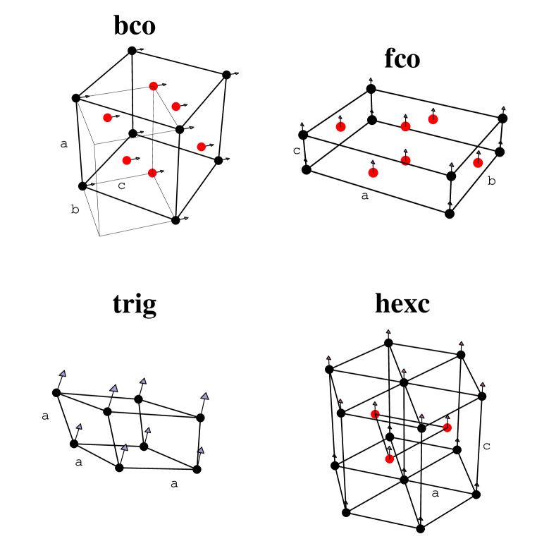
FIG. 1.: Geometries of the first four lattice structures considered in the search for the energy minimum. For bco the situation at the fcc-bco transition is shown: when a small dipole moment is introduced in a nonpolar fcc crystal, polarization along $[110]$ is preferred and the crystal contracts in this direction. Thick and thin lines mark the conventional unit cells of fcc and bco, respectively. Red particles lie on the face centers for fcc and fco and at half height ($z=c/2$) for hexc.

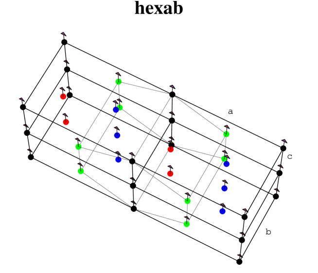
FIG. 2.: The “hexab” crystal structure which arises from a distortion of a hexagonal close packed lattice polarized in a nearest-neighbor direction within the hexagonal plane. It is an orthorhombic structure with three additional basis particles shown in red (${\boldsymbol{\tau}}_{1}$), green (${\boldsymbol{\tau}}_{2}$), and blue (${\boldsymbol{\tau}}_{3}$) with coordinates as given in the main text. Four orthorhombic unit cells are shown. The thin lines mark the hexagonal unit cell that is recovered for the special axis ratio $c/a=1/\sqrt{3}$.

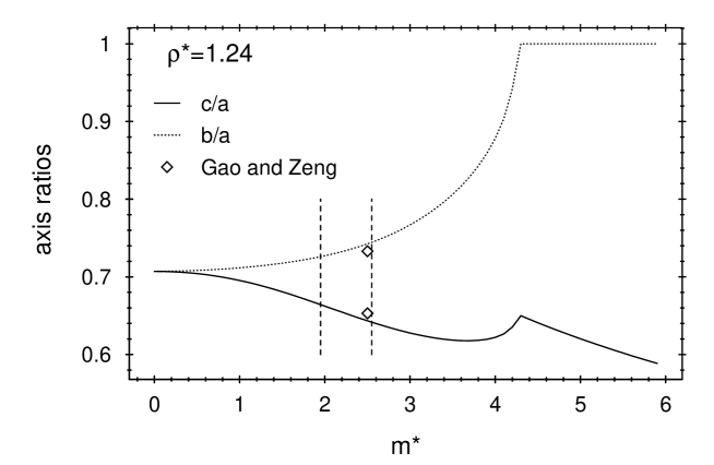
FIG. 3.: Axis ratios of the bco phase of a Stockmayer solid at $T=0$ and $\rho^{\ast}=1.24$ as a function of the dipole moment. For $m^{\ast}=0$ one has $c/a=b/a=1/\sqrt{2}$ corresponding to fcc. The diamonds denote simulation results of Gao and Zeng [23] for $\rho^{\ast}=1.24$, $m^{\ast}=2.5$, and $T^{\ast}=0.7$. At $m^{\ast}_{c}\simeq 4.25$ a continuous transition to bct takes place. Note that for $m^{\ast}<1.95$ the hexc structure is slightly more stable than bco, while for $m^{\ast}>2.55$ gas-solid phase separation occurs. Thus for this density bco is stable within the indicated window and metastable outside.

FIG. 4.: Ground state phase diagram of the Stockmayer model. The solid (dotted) line denotes first (second) order transitions. The dashed line indicates the global minimum of the energy per particle over all densities. The unlabeled area to the left of this line is a two-phase region where an infinitely diluted gas coexists with the solid. The maximum of the pressure $p=\rho^{2}\partial U/\partial\rho$ in the depicted parameter range occurs in the lower right corner where $p\simeq 500\epsilon/\sigma^{3}$. Using parameter values for argon this corresponds to about 20 GPa which is accessible in a laboratory.

FIG. 5.: Axis ratios of the bco structure of a Stockmayer solid at $\rho^{\ast}=1.24$ and $T^{\ast}=0.7$ calculated from density-functional theory. Ferroelectric order sets in for $m^{\ast}\gtrsim 0.67$. The detailed behavior near this point could not be clarified due to numerical problems.

FIG. 6.: Phase diagram of the Stockmayer fluid as calculated from density-functional theory for $m^{\ast}=2$. The ferroelectric solid has hexc structure. The dotted line indicates the gas–ferroelectric liquid–ferroelectric solid triple temperature. The dashed lines are the corresponding phase boundaries if an fcc solid is assumed. The unlabeled areas are two-phase regions.

FIG. 7.: Ground state phase diagram of the dipolar soft sphere model for $m^{\ast}=1$. The meaning of the line styles is the same as in Fig. 4. The abbreviations for the various crystal structures are explained in the main text. The unlabeled areas are two-phase regions. The plots in the middle and at the bottom are magnifications of the regions around $n=12$ and near the hard sphere limit $n=\infty$, respectively. The phase diagram for other dipole moments $m^{\ast}$ can be inferred from the one given here by rescaling the reduced density according to $\rho^{\ast}/{m^{\ast}}^{6/(n-3)}$. In the limit $\rho^{\ast}\to\infty$ the upper bco phase turns into fcc continuously.

FIG. 8.: Interaction potential between parallel chains of dipolar soft spheres, with a longitudinal shift of half the intrachain particle distance $a$, for different values of the exponent $n$ as a function of the chain separation $r$. The plot is for $m^{\ast}=1$; corresponding curves for other dipole moments can be obtained by rescaling the distance with ${m^{\ast}}^{-2/(n-3)}$ and the energy with ${m^{\ast}}^{2n/(n-3)}$.

REFERENCES

- [1] B. Groh and S. Dietrich, in New Approaches to Problems in Liquid State Theory, Vol. 529 of NATO Science Series, edited by C. Caccamo, J.-P. Hansen, and G. Stell (Kluwer, Dordrecht, 1999), pp. 173–196, and references therein.
- [2] P. Teixeira, J. Tavares, and M. T. da Gama, J. Phys.: Condens. Matter 12, 411 (2000).
- [3] R. van Roij, Phys. Rev. Lett. 76, 3348 (1996).
- [4] J. Shelley, G. Patey, D. Levesque, and J. Weis, Phys. Rev. E 59, 3065 (1999).
- [5] D. Wei and G. Patey, Phys. Rev. Lett. 68, 2043 (1992).
- [6] J. Weis, D. Levesque, and G. Zarragoicoechea, Phys. Rev. Lett. 69, 913 (1992).
- [7] M. Stevens and G. Grest, Phys. Rev. E 51, 5976 (1995).
- [8] J. Weis and D. Levesque, Phys. Rev. Lett. 71, 2729 (1993).
- [9] M. Stevens and G. Grest, Phys. Rev. E 51, 5962 (1995).
- [10] B. Groh and S. Dietrich, Phys. Rev. Lett. 72, 2422 (1994).
- [11] B. Groh and S. Dietrich, Phys. Rev. E 50, 3814 (1994).
- [12] S. Klapp and F. Forstmann, J. Chem. Phys. 106, 9742 (1997).
- [13] R. Sear, Phys. Rev. Lett. 76, 2310 (1996).
- [14] M. Osipov, P. Teixeira, and M. T. da Gama, Phys. Rev. E 54, 2597 (1996).
- [15] B. Groh and S. Dietrich, Phys. Rev. E 54, 1687 (1996).
- [16] S. Klapp and F. Forstmann, Europhys. Lett. 38, 663 (1997).
- [17] S. Klapp and F. Forstmann, J. Chem. Phys. 109, 1062 (1998).
- [18] S. Klapp and G. Patey, J. Chem. Phys. 112, 10949 (2000).
- [19] R. Tao and J. Sun, Phys. Rev. Lett. 67, 398 (1991).
- [20] J. Martin, R. Anderson, and C. Tigges, J. Chem. Phys. 108, 3765 (1998).
- [21] T. Chen, R. Zitter, and R. Tao, Phys. Rev. Lett. 68, 2555 (1992).
- [22] U. Dassanayake, S. Fraden, and A. van Blaaderen, J. Chem. Phys. 112, 3851 (2000).
- [23] G. Gao and X. Zeng, Phys. Rev. E 61, 2188 (2000).
- [24] J. Weis and D. Levesque, Phys. Rev. E 48, 3728 (1993).
- [25] E. Lomba, J. Weis, and C. Tejero, Phys. Rev. E 58, 3426 (1998).
- [26] J. Fernández and J. Alonso, Phys. Rev. B 62, 53 (2000).
- [27] B. Groh and S. Dietrich, Phys. Rev. E 53, 2509 (1996).
- [28] B. Groh and S. Dietrich, Phys. Rev. E 57, 4535 (1998).
- [29] A. Smith and N. Ashcroft, Phys. Rev. B 38, 12942 (1988).
- [30] B. Nijboer and F. de Wette, Physica 23, 309 (1957).
- [31] J. Slater, Insulators, Semiconductors, and Metals (McGraw-Hill, New York, 1967).
- [32] A. Denton and N. Ashcroft, Phys. Rev. A 39, 4701 (1989).
- [33] W. Curtin and N. Ashcroft, Phys. Rev. Lett. 56, 2775 (1986).
- [34] S. Gay, P. Beale, and J. Rainwater, J. Chem. Phys. 109, 6820 (1998).
- [35] R. Rosensweig, Ferrohydrodynamics (Cambridge University Press, Cambridge, 1985).
- [36] Electro-Rheological Fluids, Magneto-Rheological Suspensions and Associated Technology, edited by W. A. Bullough (World Scientific, Singapore, 1996).
- [37] E. Dubois, R. Perzynski, F. Boué, and V. Cabuil, Langmuir 16, 5617 (2000).
- [38] E. Lemaire, G. Bossis, and Y. Grasselli, Langmuir 8, 2957 (1992).
- [39] J. Woestman and A. Widom, Phys. Rev. E 48, 1995 (1993).
- [40] L. Marshall, C. Zukoski, and J. Goodwin, J. Chem. Soc. Faraday Trans. I 85, 2785 (1989).
- [41] D. Adams and I. McDonald, Mol. Phys. 32, 931 (1976).
- [42] C. Kittel, Einführung in die Festkörperphysik, 12th ed. (R. Oldenbourg, Munich, 1999).