Scattering properties of a cut-circle billiard waveguide with two conical leads

Abstract

We examine a two-dimensional electron waveguide with a cut-circle cavity and conical leads. By considering Wigner delay times and the Landauer-Büttiker conductance for this system, we probe the effects of the closed billiard energy spectrum on scattering properties in the limit of weakly coupled leads. We investigate how lead placement and cavity shape affect these conductance and time delay spectra of the waveguide.

PACS numbers: 73.50.Bk, 73.23.Ad, 05.60.Gg, 05.45.Mt

I Introduction

The scattering properties of ballistic electron waveguides have been studied by a number of authors, but primarily in the semi-classical regime, where resonances strongly overlap [1], [2]. Several experiments [3] have shown that the shape of the waveguide cavity can strongly affect the conductance, depending on whether the shape induces integrable or chaotic motion [4]. In this paper, we investigate the scattering properties of an electron waveguide whose scattering cavity strongly resembles that of a quantum dot. We investigate this system in a regime where the resonances are well separated in energy, and we look at the effect of distortions in shape and changes of lead placement, which change the symmetry of the scattering cavity, on the behavior of the scattering resonances.

The geometry of the waveguide we consider in this paper is shown in Fig. 1. The scattering system consists of a cavity with two cone shaped leads attached, which we will treat as infinitely long. The walls of both the cavity and the leads are assumed to be infinitely hard (infinite potential) walls. The cavity has the shape of a circle of radius $R$, but with a segment of the wall, subtended by an angle $\omega$, replaced by a flat segment which we call the cut. The opening angles of the leads are $\Delta\theta_{1}$ and $\Delta\theta_{2}$. The angular positions of the center of the cut and the center of the lead openings are denoted by $\zeta$, $\theta_{1}$, and $\theta_{2}$, respectively.

The effect of conical leads has already been studied in earlier works (e.g., Ree and Reichl [5], Persson et al. [6], and Berggren, Ji, and Lundberg [7]). Compared to straight leads (which have most commonly been used in publications on waveguides), conical leads are more similar to the electron sea which provides the source of electrons in most experiments. As shown in Ref. [5], conical leads allow tunneling resonances through the waveguide cavity for energy regimes in which conduction is prohibited for straight leads.

A classical particle moving in a closed billiard whose shape is that of a circle with a cut (the shape of our cavity) will display a rich range of chaotic behavior as the size of the cut is varied [8]. Quantum signatures of the classical chaos in this billiard have been studied in Ref. [9]. One question we will be interested in is how well the scattering process can probe this dynamics of the closed cavity. In the low-energy regime we will consider, we expect that the waveguide will exhibit well-separated Fano resonances at energies close to the energy eigenvalues of the closed billiard.

Beyond simply allowing to probe eigenenergies of the closed billiard as scattering resonances, lead placement itself can alter the symmetry properties of the closed billiard. We will study the effect of symmetries by investigating how the positions of the leads affect the behavior of the Fano resonances.

In Sec. 2, we will discuss cavity states and the scattering states that are used to obtain the scattering S-matrix for a system with conical leads. In Sec. 3, quantum properties of the closed circular cavity with a cut will be reviewed. In Secs. 4 and 5, we will look at the behavior of conductance and Wigner delay times for waveguides with full-circle and cut-circle cavities. Leads will be attached to cavities symmetrically or asymmetrically. Finally, in Sec. 6, we will summarize our results. A short discussion of the numerical method used for our computations is given in the Appendix.

II Scattering wavefunction and S-matrix

Matter waves inside the waveguide pictured in Fig. 1 are governed by the Schrödinger equation, which, in polar coordinates, takes the form

$$({\nabla}^{2}+k^{2}){\Psi}(\rho,\varphi)={\biggl{(}}{{\partial}^{2}\over{\partial}{\rho}^{2}}+{1\over{\rho}}{{\partial}\over{\partial}{\rho}}+{1\over{\rho}^{2}}{{\partial}^{2}\over{\partial}{\varphi}^{2}}+{2mE\over{\hbar}^{2}}{\biggr{)}}{\Psi}(\rho,\varphi)=0.$$ (1)

Here, $k=\sqrt{2mE/{\hbar}^{2}}$ is the wavevector of the particle wave, $m$ is the particle mass, $\hbar$ is Planck’s constant, and $E$ is the energy. The geometry of the system, which determines its scattering properties, is taken into account by the boundary condition that the scattering wavefunction $\Psi$ vanish on the walls.

The solution $\Psi$ is computed numerically by expanding it into suitable basis functions, and determining the expansion coefficients from the Schrödinger equation and its boundary conditions by the method described in the Appendix. Below, we will discuss the expressions for $\Psi$ in the different regions of our system. In Sec. II A, we look at the wavefunction inside the cavity. The wavefunction inside the leads is considered in Sec. II B, where we will also define the scattering S-matrix of the waveguide.

A Cavity states

In the interior region of the cavity, the solution of Eq. (1) can be written as

$$\Psi={\sum_{\gamma=-n_{\gamma}+1}^{n_{\gamma}}}c_{\gamma}f_{\gamma}\>.$$ (2)

Here, the $f_{\gamma}$’s are suitable expansion functions. The $c_{\gamma}$’s are the expansion coefficients, which must be determined from the boundary conditions, by the procedure described in the Appendix. The cutoff number $n_{\gamma}$ has to be chosen in a proper way to achieve optimal numerical accuracy within a reasonable computation time. We used $n_{\gamma}=90$ for all computations presented here.

For the functions $f_{\gamma}$, several choices are possible in principle. For our geometry, it proved to be numerically most efficient to use solutions of the Helmholtz equation [$(\nabla^{2}+k^{2})f_{\gamma}=0$, without boundary conditions] which can be separated into polar coordinates, ($\rho,\varphi$). These functions take the form

$$f_{\gamma}(\rho,\varphi)=J_{|\gamma|}(k\rho)\>e^{i\gamma\varphi}\>,$$ (3)

where $J_{|\gamma|}$ denotes the Bessel function of order ${|\gamma|}$.

B Lead states

For waveguide scattering problems, it is usual to express the properties of the system in terms of an S-matrix, which contains reflection and transmission amplitudes from incoming channels to outgoing channels in the leads. Before we can properly define the S-matrix for our system, we first have to specify what we mean by incoming and outgoing channels (also called “modes”) in this particular case.

Following the conventions from scattering problems with straight leads, we require that an incoming (outgoing) mode $\chi^{-}$ ($\chi^{+}$) is a solution of

$$(\nabla^{2}+k^{2})\chi^{\pm}=0$$ (4)

which is separable into coordinates longitudinal and transversal to the lead walls. As a further condition, the transverse part has to be a standing wave vanishing on the walls and the longitudinal part describes a wave propagating towards (away from) the cavity.

For the conical shape of our leads, the longitudinal and transversal coordinates are just the polar coordinates $\rho$ and $\varphi$, respectively. Thus, the separation ansatz with a standing wave in the transverse direction ($\alpha=1,2,\ldots$) takes the form

$${\chi}_{\alpha}^{i\pm}=Nu_{\alpha}^{i\pm}(\rho)~{}\sin\left[{{\alpha}{\pi}{\left(\varphi-\theta_{i}+{\Delta\theta_{i}\over 2}\right)}\over{\Delta}{\theta_{i}}}\right],$$ (5)

where $\theta_{i}$ locates the angular position of the center of the $i$th lead, $R\leq\rho<\infty$, and $\theta_{i}-\Delta\theta_{i}/2\leq\varphi<\theta_{i}+\Delta\theta_{i}/2$ ($i=$1, 2 for leads 1 and 2, respectively). $N$ is a (yet unknown) constant factor.

Inserting this into Eq. (4) leads to an equation for the radial part of the wavefunction,

$$\left[{\rho^{2}}{{\partial}^{2}\over\partial{\rho^{2}}}+\rho{\partial\over{\partial\rho}}-\left(\frac{\alpha\pi}{\Delta\theta_{i}}\right)^{2}+k^{2}\rho^{2}\right]u^{i\pm}_{\alpha}(\rho)=0\>.$$ (6)

This is the Bessel differential equation and therefore $u^{i\pm}_{\alpha}(\rho)$ can be expressed as a linear combination of Bessel functions, $J_{\alpha\pi/\Delta\theta_{i}}(k\rho)$ and $Y_{\alpha\pi/\Delta\theta_{i}}(k\rho)$. Since we required that the longitudinal part represent a propagating wave, we write the radial solution in terms of Hankel functions,

$$u_{\alpha}^{\pm}(\rho)=H^{\pm}_{\frac{\alpha\pi}{\Delta\theta_{i}}}(k\rho)=J_{\frac{\alpha\pi}{\Delta\theta_{i}}}(k\rho)\pm iY_{\frac{\alpha\pi}{\Delta\theta_{i}}}(k\rho)\>,$$ (7)

which approach exponential functions at infinity:

$$H^{\pm}_{\frac{\alpha\pi}{\Delta\theta_{i}}}(k\rho)\stackrel{{\scriptstyle k\rho\rightarrow\infty}}{{\rightarrow}}\sqrt{\frac{2}{\pi k\rho}}\>\exp\left\{\pm i\left[k\rho-\frac{\pi}{4}\left(2\frac{\alpha\pi}{\Delta\theta_{i}}+1\right)\right]\right\}+{\cal O}\left[\frac{1}{(k\rho)^{3/2}}\right]\>.$$ (8)

Here, we used the notation $H_{\gamma}^{+}$ ($H_{\gamma}^{-}$) for the Hankel functions of first (second) kind, of order $\gamma$.

The normalization constant, $|N|$, is calculated from the condition that each channel carry unit current, i.e., we require that

$$\left|\int_{\theta_{i}-\Delta\theta_{i}/2}^{\theta_{i}+\Delta\theta_{i}/2}\rho\>d\varphi\>j^{i\pm}_{\rho}\right|=1.$$ (9)

Here, the longitudinal component of the probability current density, ${\bf j}^{\,i\pm}=j^{\,i\pm}_{\rho}\>{\bf e_{\rho}}+j^{\,i\pm}_{\varphi}\>{\bf e_{\varphi}}$, is given by

$$j^{\,i\pm}_{\rho}=\frac{i\hbar}{2m}\left[\left(\frac{\partial\chi^{i\pm}}{\partial\rho}\right)^{*}\chi^{i\pm}-\chi^{i\pm^{*}}\left(\frac{\partial\chi^{i\pm}}{\partial\rho}\right)\right].$$ (10)

This yields

$$|N|=\sqrt{\frac{\pi m}{\hbar\Delta\theta_{i}}}\>.$$ (11)

With these results, the expression for the incoming/outgoing channel $\alpha=1,2,\ldots$, corresponding to the $\alpha$th standing wave in transverse direction, becomes

$$\chi_{\alpha}^{\pm}=\frac{N}{|N|}\sqrt{\frac{m\pi}{\hbar\Delta\theta_{i}}}\;\sin\left[\frac{\alpha\pi{\left(\varphi-\theta_{i}+\frac{\Delta\theta_{i}}{2}\right)}}{\Delta\theta_{i}}\right]\>H^{\pm}_{\frac{\alpha\pi}{\Delta\theta_{i}}}(k\rho)\>.$$ (12)

To fix the overall phase factor, $N/|N|$, in Eq. (12), we require that the solution be real at the interface between the leads and the cavity. Then, if a mode is completely reflected back at this position, the corresponding reflection coefficient will be 1. This can be achieved by multiplying the modes with a complex phase factor. At $\rho=R$, the Hankel functions (the only complex factor in $\chi_{\alpha}^{i\pm}$) can be written as

$$H_{\frac{\alpha\pi}{\Delta\theta_{i}}}^{\pm}(kR)=\left|H_{\frac{\alpha\pi}{\Delta\theta_{i}}}^{\pm}(kR)\right|\>\exp\left\{\pm i\arctan\left[\frac{Y_{{\alpha\pi}/{\Delta\theta_{i}}}(kR)}{J_{{\alpha\pi}/{\Delta\theta_{i}}}(kR)}\right]\right\}\>.$$ (13)

Because we want the probability amplitude at this position to be real, we will use the complex phase factor

$$\frac{N}{|N|}=\exp\left\{\mp i\>\arctan\left[\frac{Y_{{\alpha\pi}/{\Delta\theta_{i}}}(kR)}{J_{{\alpha\pi}/{\Delta\theta_{i}}}(kR)}\right]\right\}\>.$$ (14)

Then, the final form of the incoming and outgoing propagating modes in channel $\alpha$ becomes

$$\chi_{\alpha}^{i\pm}(\rho,\varphi)=\sqrt{\frac{m\pi}{\hbar\Delta\theta_{i}}}\;\exp\left\{\mp i\>\arctan\left[\frac{Y_{\frac{\alpha\pi}{\Delta\theta_{i}}}(kR)}{J_{\frac{\alpha\pi}{\Delta\theta_{i}}}(kR)}\right]\right\}\sin\left[\frac{\alpha\pi{\left(\varphi-\theta_{i}+\frac{\Delta\theta_{i}}{2}\right)}}{\Delta\theta_{i}}\right]\>H^{\pm}_{\frac{\alpha\pi}{\Delta\theta_{i}}}(k\rho)\>.$$ (15)

As we now have derived the expression for incoming and outgoing channels, we are finally in the position to define the S-matrix of our system. The matter wave $\Psi$ inside the leads is expanded in terms of the incoming and outgoing modes, $\chi_{\alpha}^{i-}(\rho,\varphi)$ and $\chi_{\alpha}^{i+}(\rho,\varphi)$, respectively. Then the expansion coefficients describe the probability amplitudes of reflection or transmission of the matter wave from an incoming channel to the outgoing channels. More precisely, if the electron is incident in lead 1 and channel $\beta$, the wavefunction in the leads takes the form

$$\Psi_{\beta,1}=\chi^{1-}_{\beta}+\sum_{\alpha}r_{\alpha\beta}\chi^{1+}_{\alpha}~{}~{}~{}{\rm and}~{}~{}~{}\Psi_{\beta,2}=\sum_{\alpha}t_{\alpha\beta}\chi^{2+}_{\alpha}\>.$$ (16)

Here, $\Psi_{\beta,1}$ is the state in lead 1, $\Psi_{\beta,2}$ is the state in lead 2, and $r_{\alpha\beta}~{}(t_{\alpha\beta})$ is the probability amplitude that the electron enters in channel $\beta$ and is reflected (transmitted) into channel $\alpha$. Likewise, if the electron is incident in lead 2 and channel $\beta$, the wavefunction in the leads takes the form

$${\Psi}_{\beta,2}=\chi^{2-}_{\beta}+\sum_{\alpha}r^{{}^{\prime}}_{\alpha\beta}\chi^{2+}_{\alpha}~{}~{}~{}{\rm and}~{}~{}~{}\Psi_{\beta,1}=\sum_{\alpha}t^{{}^{\prime}}_{\alpha\beta}\chi^{1+}_{\alpha}\>.$$ (17)

Here $\Psi_{\beta,2}$ is the state in lead 2, $\Psi_{\beta,1}$ is the state in lead 1, and $r^{{}^{\prime}}_{\alpha\beta}$ and $t^{{}^{\prime}}_{\alpha\beta}$ are the reflection and transmission probability amplitudes, respectively. Note that the solution $\Psi$ of Eq. (1) is not unique, but we obtain different solutions $\Psi_{\beta}$ depending on which channel $\beta$ is assumed to carry the incoming part of the matter wave.

The S-matrix connects the amplitudes of the incoming propagating electrons to the amplitudes of the outgoing propagating electrons and it is therefore constructed out of all the reflection and transmission amplitudes. Thus, the S-matrix can be written

$${\bf S}=\left(\begin{array}[]{cc}{\bf R}&{\bf T^{\prime}}\\ {\bf T}&{\bf R^{\prime}}\end{array}\right)\>,$$ (18)

where $\bf R$ and $\bf R^{\prime}$ are square matrices composed of reflection amplitudes, $r_{\alpha\beta}$ and $r^{\prime}_{\alpha\beta}$, and $\bf T$ and $\bf T^{\prime}$ are square matrices composed of transmission amplitudes, $t_{\alpha\beta}$ and $t^{\prime}_{\alpha\beta}$. The reflection and transmission amplitudes must be computed numerically (see Appendix).

III Closed cut-circle billiard

One aspect of the scattering properties of the waveguide that we wish to explore is how close a correspondence there is between the Fano scattering resonances and the eigenstates of a closed version of the waveguide cavity. In this section, we therefore describe some features of these eigenstates as the cut size on the cut-circle billiard is changed.

The Schrödinger equation [Eq. (1)] for a quantum particle in a closed full-circle billiard is separable, with one part describing the radial and the other part the azimuthal motion. The (discrete) energy spectrum can be labeled with two good quantum numbers. One of them, $n=1,2,...$, is associated with radial motion, and the other, $l=0,{\pm}1,{\pm}2,...$, with the angular motion. The eigenfunctions are

$$\Psi_{l,n}=J_{|l|}\left(k_{|l|,n}~{}\rho\right)e^{il\varphi}\>,$$ (19)

where $J_{|l|}$ is the Bessel function of order $|l|$ and $(k_{|l|,n}R)$ is its $n$th zero (i.e., $J_{|l|}$ vanishes at $\rho=R$). The corresponding eigenenergies $E_{|l|,n}$ are then calculated via $E=\hbar^{2}k^{2}/(2m)$. The energy eigenstates of the circle billiard with angular momentum $|l|{\geq}1$, corresponding to clockwise or counter clockwise rotation of the matter wave, produce two-fold degenerate eigenenergies. Only the eigenenergies with $l=0$ are non-degenerate.

If we apply a cut to the closed system, the classical dynamics of the particle exhibits hard chaos [8], as long as ${\omega}{\leq}180^{\circ}$. Looking at the quantum properties, we observe a splitting of the degenerate eigenenergies as the cut is inserted. The absence of degenerate eigenvalues (level repulsion) is a well-known quantum feature of classically chaotic systems (see, e.g., Ref. [10]).

Examining the quantum properties of the cut-circle billiard in more detail, we show how five of the energy levels of the cut billiard behave as the cut size is varied from ${\omega}=50^{\circ}$ to ${\omega}=70^{\circ}$ in Fig. 2. The states shown are continuations of the circle cavity degenerate pairs $(l=3,n=2)$, $(l=6,n=1)$, and one of the pair, $(l=1,n=3)$.

Here and in later numerical computations, we are using dimensionless variables. The dimensionless energy $\epsilon$ is given by

$${\epsilon}={mR^{2}\over{\hbar}^{2}}E={(kR)^{2}\over 2}={{\kappa}^{2}\over 2},$$ (20)

where ${\kappa}=kR$ is a dimensionless wavevector. To get an idea of how this translates to the physical dimensions of our system, consider an electron density of $n\>{\approx}\>4{\times}10^{11}\>{\rm cm}^{-2}$, which is a typical value measured for a two dimensional electron gas in a GaAs/Al_0.3Ga_0.7As heterostructure [11]. The corresponding Fermi wavevector is $k_{f}={\sqrt{2\pi n}}\>{\approx}\>1.6{\times}10^{8}\>{\rm m}^{-1}$, the Fermi energy $E_{f}=\pi\hbar^{2}n/m\approx 0.014\>{\rm eV}$ (for an effective electron mass in GaAs of $m=0.067m_{e}$). This yields for $\epsilon=100$, which is the maximum energy we used in the computations, $R\>\approx\>90\>{\rm nm}$.

In Fig. 2, we observe a (distant) avoided crossing, which occurs between states 2b and 3a in the interval $\omega=53^{\circ}$ to $\omega=63^{\circ}$. We also see an actual crossing in this plot. This occurs between the states labeled 2a and 2b at about $\omega=65^{\circ}$.

However, as discussed in Ref. [12], separate eigenvalues of a generic Hamiltonian can in general only be brought to coincide if at least three parameters are varied. Thus, at first sight, we would expect another level repulsion instead of the actual crossing, since we only vary $\omega$. Yet we ignored that the Hamiltonian of the cut-circle is not completely “generic”. Even if the cut is inserted, the system retains parity symmetry with respect to an axis perpendicular to the cut, i.e.,

$$P_{\zeta}\Psi(\rho,\varphi)\equiv\Psi(\rho,\zeta-\varphi)=\Psi(\rho,\varphi)\>,$$ (21)

where $P_{\zeta}$ is the parity operator for a symmetry axis through the center of the cavity, at angle $\zeta$ (i.e., the angle at which the center of the cut is placed). Because of parity symmetry, we have two different symmetry classes, namely the classes formed by even and odd states. Since parity is a discrete symmetry, states of one class cannot interact with states of the other, thus both classes are completely independent of each other. Therefore, crossings between states of different parity may occur. Only within each parity class, i.e., among states with the same parity, crossings remain impossible.

In Fig. 3, we show energy eigenstates corresponding to the eigenvalues 2a, 2b, and 3a in Fig. 2, for three different cut sizes taken before the avoided crossing, between the avoided and actual crossings, and after the actual crossing. It can be seen that 2a has even parity, and 2b and 3a both have odd parities. This explains why 2a and 2b can undergo the crossing, whereas a crossing between 2b and 3a is avoided.

We also see that the state 2a, which does not participate in the avoided crossing and undergoes the crossing with 2b, remains unchanged. However, states 2b and 3a, which do undergo an avoided crossing, become mixed and loose their original identities. The mutual parity of states 2b and 3a allows them to couple, whereas this is impossible for states 2a and 2b with differing parities.

IV Waveguide with a circle cavity

If we attach leads to the circle billiard, we have a matter waveguide and the eigenstates of the billiard become unstable and may decay. These unstable states strongly affect the scattering dynamics of the waveguide. They appear as resonances in the transmission probabilities through the waveguide,

$$T_{\beta}=\sum_{\alpha}|t_{\alpha\beta}|^{2}\>,$$ (22)

for incoming mode $\beta$ in lead 1, where $\alpha$ runs over the outgoing modes in lead 2. We can examine the individual $T_{\beta}$’s or consider their sum over all possible incoming modes in lead 1, which is proportional to the Landauer-Büttiker conductance [13],

$$G=\frac{2e^{2}}{h}\sum_{\beta}T_{\beta}\>.$$ (23)

As shown in Ref. [5], there is an energy range where, for conical leads, mode $\beta$ has nonzero transmission, whereas for straight leads with the same opening angles it would still be evanescent. This occurs for energies too small for the $\beta$th transverse standing wave to fit into the lead opening at the junction to the cavity, such that the wave has to “tunnel” into the cavity. The condition for this tunneling (see Ref. [5]) is $k<\beta\pi/d_{i}$, if $d_{i}=2R\sin(\Delta\theta_{i}/2)$ is the width of the lead opening (for opening angle $\Delta\theta_{i}$). Thus, tunneling occurs for energies such that

$$\epsilon<\tilde{\epsilon}_{\beta}=\frac{\beta^{2}\pi^{2}R^{2}}{2d_{i}^{2}}=\frac{\beta^{2}\pi^{2}}{8\sin^{2}(\Delta\theta_{i}/2)}\>,$$ (24)

where $\epsilon$ is the dimensionless energy defined in Eq. (20).

In addition to the transmission probabilities and Landauer-Büttiker conductance, it is useful to look at the Wigner delay times,

$$\tau_{n}^{W}=\hbar\frac{\partial\theta_{n}}{\partial E}\>,$$ (25)

where $\theta_{n}$ are the phases of the S-matrix eigenvalues $s_{n}=e^{i\theta_{n}}$. The Wigner delay times are a measure of the time delay of the electron due to the presence of the cavity. In the following plots, we will use dimensionless delay times

$$\tau_{n}=\frac{\partial\theta_{n}}{\partial\epsilon}=\frac{\hbar\tau^{W}_{n}}{m_{e}^{*}R^{2}}\>.$$ (26)

(For $R\approx 100\>{\rm nm}$, $\tau_{n}\approx 20$, and $m_{e}^{*}=0.067m_{e}$, the Wigner delay time is of the order of 0.1 ns.) From Ref. [14] it is clear that peaks in the Wigner delay time correspond to resonances and poles of the scattering matrix in the complex energy plane. Therefore we can use peaks in the delay time spectra to indicate the resonances of our system.

A Symmetric placement of leads

In Fig. 4, we show numerical data obtained for an electron waveguide with a circle cavity with symmetrically placed leads, one at $\theta_{1}=0^{\circ}$ and the other at $\theta_{2}=180^{\circ}$. Both leads subtend the same angle $\Delta\theta_{1}=\Delta\theta_{2}=20^{\circ}$. The dimensionless energy $\epsilon$ is varied in steps of 0.5.

The transmission probability in Fig. 4(a) shows the quantities $T_{\beta}$ for incoming modes $\beta=1,2$ in lead 1. The first mode ($\beta=1$) starts transmitting (i.e., becomes significantly larger than zero) at about $\epsilon\approx 20$. The second mode starts transmitting too closely below 100 to be visible in the plot. The transmission for higher modes is zero everywhere in the energy interval below 100, and therefore these modes were not included in the computations or the plot.

The threshold energies $\tilde{\epsilon}_{\beta}$, for which the modes would start propagating in the case of straight leads with $\Delta\theta=20^{\circ}$, are $\tilde{\epsilon}_{1}=40.91$, and $\tilde{\epsilon}_{2}=163.66$ for the first two channels. This means that for the conical leads, we observe tunneling of the first mode in the energy range between $\epsilon\approx 20$ and 40.

Examining the correspondence between eigenenergies of the closed circle (indicated by filled circles for degenerate levels and open circles for non-degenerate levels) and resonances of the open system, one finds that there is obviously a strong association. In energy intervals without eigenenergies, the transmission changes smoothly, whereas there are sharp changes close to eigenenergies. In the tunneling regime, we see peaks close to the eigenenergies. The peaks tend to be slightly shifted to the left. Above the tunneling threshold, we also observe valleys, e.g., at $\epsilon=67.5,74.7$. In this regime, most peaks and valleys in the vicinity of an eigenenergy are too close together to tell which is associated with the eigenenergy. Since the lead openings themselves alter the geometry of the system, we cannot expect the resonances to be found exactly at the same positions as the eigenenergies.

In Fig. 4(b), we plot the dimensionless delay times $\tau_{n}$. The energy derivatives at each point are approximated by carrying out two computations for each point, with energy spacing $\Delta\epsilon=10^{-5}$. Since the transmission probabilities $T_{\beta}$ vanish for $\beta\geq 3$, we only have to consider the two channels $\beta=1$ and $\beta=2$. Thus, the S-matrix is a 4x4 matrix and we get four eigenphases and four delay time curves.

Here, unlike for the transmission probabilities, we only need to look for peaks in the Wigner delay times at the resonance energies, in the tunneling as well as in the normal regime. The first two time delays display their first peak around $\epsilon\approx 15$, the others at $\epsilon\approx 75$. At these energies, the corresponding transmission probabilities are still too close to zero to produce a visible peak in Fig. 4(a). This shows that the delay times are a more sensitive indicator of resonances than the $T_{\beta}$’s.

We see that the degenerate eigenenergies of the circle billiard do not produce double resonances when leads are attached at the special angles $\theta_{1}=0^{\circ}$ and $\theta_{2}=180^{\circ}$. Every eigenenergy of the circle billiard is associated only with a single delay time peak. Although placing leads to the circle cavity destroys its radial symmetry, the breaking of the degeneracy is not observed in this case.

B Asymmetric placement of leads

In Fig. 5, we show the same waveguide, but with asymmetric placement of leads instead of the symmetric placement we had in Fig. 4. Lead 1 is placed at $\theta_{1}=0^{\circ}$ and lead 2 at $\theta_{2}=125^{\circ}$.

Now we not only see again the close correspondence between delay time peaks and eigenenergies of the circle, but we also observe double peaks at most of the degenerate billiard eigenenergies, most evidently at $\epsilon=$24.6, 28.8, 35.4, 38.5, and 49.4. At higher energies, the observation of double peaks is more difficult because the second mode starts transmitting. (Some of its first peaks are too small to be seen in the plot, but can be found by looking at the data file.) Many of the double peaks show a small energy spacing: One peak is slightly shifted to smaller energies, the other one to higher energies. Here, the degeneracy is obviously broken by the addition of the leads. For the non-degenerate eigenenergies on the other hand, no splitting can be observed. Especially at $\epsilon=37.4$, this becomes very obvious.

The difference between this case and the previous case with symmetric lead placement ($\theta_{2}=180^{\circ}$) is that, for symmetric placement, we had two discrete symmetries, namely invariance under the parity transformations $P_{0^{\circ}}$ and $P_{90^{\circ}}$ [where the parity operators are defined as in Eq. (21)]. When the leads are placed asymmetrically, the symmetry under $P_{0^{\circ}}$, with respect to the axis bisecting both leads, is destroyed, and we are only left with one parity symmetry under $P_{62.5^{\circ}}$. The breaking of one parity symmetry seems to be the reason for the splitting of resonances seen in Fig. 5(b).

C Numerical accuracy

To get an estimate of the numerical error, the sum of the absolute values squared of all reflection and transmission amplitudes was calculated. Due to the unitarity of the S-matrix, this value has to be the dimension of the S-matrix, which is 4 here. The relative error,

$$1-\frac{1}{4}\sum_{\alpha,\beta=1}^{2}(|r_{\alpha\beta}|^{2}+|t_{\alpha\beta}|^{2}+|r^{{}^{\prime}}_{\alpha\beta}|^{2}+|t^{{}^{\prime}}_{\alpha\beta}|^{2})\>,$$ (27)

was usually smaller than 0.2% for the individual data points. The errors of the absolute values of the S-matrix eigenvalues (which should be 1) were of the same order of magnitude. For the delay times, there is no easy way to estimate the error.

The most crucial factor determining numerical accuracy was found to be the number $2n_{\gamma}$ of parameters (expansion coefficients $r_{\alpha\beta},t_{\alpha\beta},b_{\nu\beta}$) used to approximate the total wavefunction $\Psi$ of our system [see Eqs. (16), (A10), and (A19)]. An estimate for a suitable choice of this number can be found by comparing the Fermi wavelength, $\lambda_{f}=2\pi/k_{f}$, to a typical length scale of the system, e.g., the length of the boundary $\approx 2\pi R$ (for zero or small cut size). If we assume that the total wavefunction of our system varies rather smoothly on a length scale of $\lambda_{f}$, it seems plausible that a “small” number of parameters, say about 10, should be sufficient to approximate $\Psi$ on an interval of length $\lambda_{f}$. Therefore, we expect that such a “small” multiple of $\kappa=k_{f}R=\sqrt{2\epsilon}$=“the number of $\lambda_{f}$-intervals needed to cover the cavity boundary” should give a reasonable order of magnitude estimate for $2n_{\gamma}$.

In Fig. 6, we compare the transmission spectra [Fig. 6(a)] and the spectra of the time delay sums [Fig. 6(b)] for different values of $n_{\gamma}$. As deviations are expected to be most pronounced for large cut size, the calculations shown were done exemplarily for the symmetric cut-circle waveguide to be examined in Sec. V A, at $\omega=80^{\circ}$.

We find noticeable deviations for $n_{\gamma}=30$ and, to a small extent, also for $n_{\gamma}=60$. The values for $n_{\gamma}=90$ practically coincide with those for $n_{\gamma}=120$. Therefore, in view of computation time, we used $n_{\gamma}=90$ in all computations presented in this paper.

V Waveguide with a cut-circle cavity

We now consider a waveguide with a cut-circle cavity. Fig. 7 shows the sum of the partial delay times, $\tau=\sum_{n=1}^{4}\tau_{n}$, and the Landauer-Büttiker conductance $G$. For this computation, leads and cut are placed asymmetrically. The leads are centered at $\theta_{1}=0^{\circ}$ and $\theta_{2}=166^{\circ}$, and the cut at $\zeta=225^{\circ}$. The cut size $\omega$ varies from $0^{\circ}$ (circle) to $80^{\circ}$, with step size $5^{\circ}$. The dimensionless energy $\epsilon$ is varied in steps of 0.25.

In the delay time spectrum (upper plot), we observe chains of separated double peaks, corresponding to the split-up branches of degenerate circle eigenenergies. If we compare the positions of maxima in the Wigner delay time to the positions of eigenenergies of the closed system, we find a good agreement between (open system) resonances and (closed cavity) eigenenergies.

The conductance (lower plot) shows similar features. However, the first visible chains of resonances occur at significantly higher energies than in the delay time plot. For energies between 20 and 40, both plots show basically the same structures. Above the first tunneling threshold at $\tilde{\epsilon}_{1}=40.91$, the conductance reflects the onset of “normal” (compared to tunneling) transmission of the first mode. In this energy regime, we cannot tell any more whether resonances are indicated by peaks or dips in the conductance.

We will now compare the properties of the cut-circle cavity waveguide for symmetric and asymmetric lead placements. Note, however, that although this may seem to be analogous to the analysis from the previous section (for the full-circle cavity), the insertion of the cut already leaves us with only one parity symmetry (under $P_{\zeta}$). As a result, the “symmetric” cut-circle waveguide is analogous to the asymmetric full-circle waveguide rather than to the symmetric full-circle waveguide. Finally, in the “asymmetric” cut-circle waveguide, there are no geometric symmetries present at all. Since this could not be achieved by merely placing two leads to a circle, this case has no parallel in Sec. IV.

A Symmetric placement of leads and cut

Let us examine the Wigner delay times for the energy range where we found an actual crossing and an avoided crossing in Fig. 2 for the closed cut-circle billiard. We first consider a system in which the leads are placed at $\theta_{1}=0^{\circ}$ and $\theta_{2}=120^{\circ}$, symmetrically with respect to the cut at $\zeta=240^{\circ}$. The lead openings are $\Delta\theta_{1}=\Delta\theta_{2}=16^{\circ}$. The plot of the sum $\tau$ of the Wigner delay times is shown in Fig. 8.

We observe five delay time peaks, which are Fano resonances resulting from the closed cut billiard eigenstates 1a, 1b, 2a, 2b, and 3a shown in Fig. 2. Starting from the left, we label these delay time peaks in the same manner. For cut size $\omega=20^{\circ}$, we designate the delay time peaks, going from left to right, as 1b, 2a, 2b, 3a, and 3b. 1a is the resonance chain in the upper left corner. The first two delay time peaks, 1a and 1b, are Fano resonances resulting from the circle eigenstate with $(l=3,n=2)$, the following two from $(l=6,n=1)$, and the last two, 3a and 3b, from $(l=1,n=3)$.

Again, we observe an avoided crossing between 2b and 3a, and the two delay time peaks 2a and 2b actually cross. Like for the closed cavity, the crossing is possible due to the parity symmetry of the system, which has been preserved by adding the leads symmetrically with respect to the cut. Since 2a and 2b have different parities, these eigenvalue chains are allowed to cross.

The symmetric placement of leads has not broken any additional symmetries. Only the energies and cut sizes at which the avoided crossing and actual crossing take place are slightly shifted from the case of the closed cut billiard.

B Asymmetric placement of leads and cut

In Fig. 9 we show the same Fano resonances as in Fig. 8, but for asymmetric placement of leads. Now we place the leads at $\theta_{1}=0^{\circ}$ and $\theta_{2}=166^{\circ}$ and the cut at $\zeta=225^{\circ}$.

The crossing of resonances 2a and 2b, which occurred for the symmetric leads and for the closed cut-circle billiard, has now become an avoided crossing. (In fact we now have a sequence of two closely spaced avoided crossings, similar to the case studied in Ref. [10].) Here, the parity symmetry of the closed system is destroyed by placing the leads asymmetrically. Therefore, in the asymmetric open system, we no longer have two separate classes of states (namely states of even and odd parity) and the crossing, which was possible in the closed system and in the symmetric open system, is avoided here.

C Cavity wavefunctions

We now look at the distribution of electron probability in the cavity at the resonance energies. This is shown in Fig. 10 for the asymmetric system. A three-way avoided crossing has mixed the resonance states, and has destroyed the identity they had for smaller cut size. The upper row displays the four states before the avoided crossing, which still reflect the quantum numbers of the associated circle states very well. For the middle row, the character of states 2a, 2b, and 3a has been changed. Only the resonance state 1b, which never comes really close to the crossing region, has preserved its characteristic structure (two rings with six peaks each) quite well. In the bottom row, after the second avoided crossing, 2a and 2b have mixed even further.

VI Conclusion

In this paper, we investigated a waveguide with a cut-circle cavity by calculating conductances and Wigner delay times. We attached conic leads to the cavity in two ways, symmetrically and asymmetrically. We observed two kinds of avoided crossings when the leads were placed asymmetrically, breaking the parity symmetry of the closed cavity. One avoided crossing was due to the chaos of the closed cavity, i.e., due to level repulsions between states in the same symmetry class, which are known to occur for fully chaotic systems. The other avoided crossing was due to the breaking of the discrete symmetry (the parity in our case) by placing leads asymmetrically (see Fig. 9).

There is now great interest in exploring the effects of underlying chaos on the dynamics of open quantum systems. However, open quantum systems must make contact with the outside world. This contact itself may induce some of the signatures of chaos. This fact has also been studied extensively by Jung and Seligman [15] for classical scattering systems. The avoided crossing between 2a and 2b, shown in Fig. 9, provides another example of this effect.

A Numerical method

1 Basic concept

In order to obtain an explicit expression for the S-matrix, we need to find the stationary solutions $\Psi$ of Eq. (1). This can only be done numerically for our system. For that purpose, we use the boundary integral method described in Ref. [16]. Below, we will give an outline of this method adapted to our particular problem.

The boundary integral method is based on the use of Green’s Theorem, which, for two functions $f$ and $g$, states that

$$\oint_{\Gamma}dl\left(f{\frac{\partial g}{\partial n}}-{\frac{\partial f}{\partial n}}{g}\right)=\int_{A}dA^{\prime}({f}{\nabla}^{2}{g}-{g}{\nabla}^{2}{f})\>,$$ (A1)

if $\Gamma$ is a closed contour confining an area $A$, $l$ is the longitudinal coordinate along $\Gamma$, and $n$ is the normal coordinate. For the boundary integral method, we choose for the functions $f$ and $g$ the wavefunction $\Psi$ and a weight function $\Phi$ that satisfies the Helmholtz equation

$${\nabla}^{2}{\Phi}=-k^{2}\Phi\>.$$ (A2)

Then, since $\Psi$ is a solution of the Schrödinger equation [Eq. (1)], i.e., $\Psi$ also satisfies ${\nabla}^{2}{\Psi}=-k^{2}\Psi$, the right hand side of Eq. (A1) is identically zero. Therefore we get

$$\oint_{\Gamma}dl\left(\Psi{\frac{\partial\Phi}{\partial n}}-{\frac{\partial\Psi}{\partial n}}{\Phi}\right)=0\>$$ (A3)

as the basic equation of this numerical approach. (Note that the difference between $\Psi$ and $\Phi$ is that there are no boundary conditions for $\Phi$, whereas $\Psi$ has to satisfy the boundary conditions imposed by the geometry of the waveguide.)

For our problem, we choose $\Gamma$ to follow the walls of the cavity. For the places where the leads come in, $\Gamma$ is taken to be the continuation of the circular wall segments in order to construct a closed contour. Then, Eq. (A3) allows us to obtain the S-matrix and the probability distribution inside the cavity for any incoming particle energy. This is done by inserting (approximate) expansions of $\Psi$ with, say, $n_{\rm cutoff}$ yet unknown expansion coefficients. As we need $n_{\rm cutoff}$ equations to solve for these expansion coefficients, we apply Eq. (A3) with sufficiently many different weight functions $\Phi_{n}$ ($n=1,\ldots,n_{\rm cutoff}$).

In principle, there are several choices possible for the $\Phi_{n}$’s, as long as they satisfy Eq. (A2). For numerical convenience, we used the same functions as for the expansion of $\Psi$ inside the cavity, namely $\Phi_{\gamma}=f_{\gamma}$ with the $f_{\gamma}$’s given by Eq. (3), where $\gamma=-n_{\gamma}+1,\ldots,n_{\gamma}$ (i.e., $n_{\rm cutoff}=2n_{\gamma}$). For $n_{\gamma}$, we also used the same value as in Sec. II A, $n_{\gamma}=90$, which allows us to determine $n_{\rm cutoff}=180$ expansion coefficients.

2 S-matrix

In order to compute the S-matrix, we split up $\Gamma$ into parts $C_{1},C_{2}$ across the lead openings, $P_{1},P_{2},P_{3}$ along the circular walls, and $P_{0}$ along the cut (see Fig. 11).

We first regard a part $I_{C}$ of the integral in Eq. (A3), for which we only integrate over the lead openings $C_{1}$ and $C_{2}$ instead of $\Gamma$. Inserting for $\Phi$ the $f_{\gamma}$’s and for $\Psi$ its expansion into lead channels from Eq. (16) (for an electron incident in channel $\beta$ in lead 1), we obtain

$$I_{C} = \int_{C_{1}}dl\left(\chi^{-}_{\beta}{\frac{\partial f_{\gamma}}{\partial n}}-{\frac{\partial\chi^{-}_{\beta}}{\partial n}}f_{\gamma}\right)+\sum_{\alpha}r_{\alpha\beta}\int_{C_{1}}dl\left(\chi^{+}_{\alpha}{\frac{\partial f_{\gamma}}{\partial n}}-{\frac{\partial\chi^{+}_{\alpha}}{\partial n}}f_{\gamma}\right)$$ (A5)

$$+\sum_{\alpha}t_{\alpha\beta}\int_{C_{2}}dl\left(\chi^{+}_{\alpha}{\frac{\partial f_{\gamma}}{\partial n}}-{\frac{\partial\chi^{+}_{\alpha}}{\partial n}}f_{\gamma}\right)$$

$$= (z_{0}^{1-})_{\gamma\beta}-(z_{L}^{1-})_{\gamma\beta}+\sum_{\alpha}r_{\alpha\beta}\left[(z_{0}^{1+})_{\gamma\alpha}-(z_{L}^{1+})_{\gamma\alpha}\right]$$ (A7)

$$+\sum_{\alpha}t_{\alpha\beta}\left[(z_{0}^{2+})_{\gamma\alpha}-(z_{L}^{2+})_{\gamma\alpha}\right]\>,$$

where we introduced the abbreviations

$$(z^{i\pm}_{L})_{\gamma\alpha} \equiv \int_{C_{i}}dl\>\frac{\partial\chi^{i\pm}_{\alpha}}{\partial n}f_{\gamma}\>,$$ (A8)

$$(z^{i\pm}_{0})_{\gamma\alpha} \equiv \int_{C_{i}}dl\>\chi^{i\pm}_{\alpha}\frac{\partial f_{\gamma}}{\partial n}\>,$$ (A9)

with $i=$1, 2 denoting lead 1 and 2. (For an electron incident in lead 2, the expressions look similar.)

Along the walls of the cavity, the electron wavefunction is zero, but it may have a finite slope perpendicular to the wall. We can expand this slope in terms of a complete orthonormal basis along the wall. Therefore, we can write

$$\Psi_{\beta,P_{i}} = 0\>,$$ (A10)

$$\left(\frac{\partial\Psi_{\beta}}{\partial n}\right)_{P_{i}} = \sum_{\nu}\>b^{(i)}_{\nu\beta}\;\xi^{(i)}_{\nu}(l),$$ (A11)

with some set of basis functions $\xi^{(i)}_{\nu}$ in variable $l$. The index $i=0$ is used to denote the cut, and $i=1,2,3$ denote the three different circular wall segments. We are free to choose any complete basis, and for the circular wall segments we choose a Fourier basis,

$$\xi^{(i)}_{\nu}(l)=\sqrt{\frac{2}{\Delta_{i}}}\cos{\biggl{[}}\frac{\pi\nu\left(l-{\delta}_{i}+\frac{\Delta_{i}}{2}\right)}{\Delta_{i}}{\biggr{]}}\>,$$ (A12)

where ${\delta}_{i}$ is the angular position of the center of wall segment $i=1,2,3$, $\Delta_{i}$ is its opening angle, $\nu=0,1,\ldots$, and ${\delta}_{i}-\frac{\Delta_{i}}{2}\leq l<{\delta}_{i}+\frac{\Delta_{i}}{2}$. For the cut, we could use the Fourier basis, too. However, as this results in very long computation times, a basis of small triangles proved to be more efficient. Thus, along the straight wall we use

$$\xi^{(0)}_{\nu}(l)=\frac{2(n_{\nu_{0}}+1)}{l_{0}}\left\{\begin{array}[]{lcr}l-\frac{\nu}{n_{\nu_{0}}+1}\;l_{0}&{\rm for}&\frac{\nu}{n_{\nu_{0}}+1}\;l_{0}\leq l<\frac{\nu+1/2}{n_{\nu_{0}}+1}\;l_{0}\\ \frac{\nu+1}{n_{\nu_{0}}+1}\;l_{0}-l&{\rm for}&\frac{\nu+1/2}{n_{\nu_{0}}+1}\;l_{0}\leq l<\frac{\nu+1}{n_{\nu_{0}}+1}\;l_{0}\\ 0&{\rm else}&\end{array}\right.\;,$$ (A13)

for $0\leq l<l_{0}$, where $l_{0}=2R\sin(\omega/2)$ is the length of the cut, $\omega$ is its opening angle, and $\nu=0,1,\ldots,n_{\nu_{0}}$. Now we can write down the part $I_{P}$ of the integral in Eq. (A3), for which we only integrate over the wall segments $P_{0},\ldots,P_{3}$ instead of $\Gamma$. Inserting the expansions from Eq. (A10), we get

$$I_{P}=-\sum_{i=0}^{3}\sum_{\nu}b^{(i)}_{\nu\beta}\int_{P_{i}}dl\>\xi^{(i)}_{\nu}f_{\gamma}=-\sum_{i=0}^{3}\sum_{\nu}b^{(i)}_{\nu\beta}~{}(x^{i})_{\gamma\nu}\>,$$ (A14)

with the abbreviation

$$(x^{i})_{\gamma\nu}\equiv\int_{P_{i}}dl\>\xi^{(i)}_{\nu}(l)f_{\gamma}\>.$$ (A15)

Now we can combine these results to obtain a matrix equation for the unknown expansion coefficients, which can easily be solved numerically. With the integrals $I_{C}$ and $I_{P}$, Eq. (A3) becomes $I_{C}+I_{P}=0$. Inserting Eqs. (A5) and (A14) yields (after a slight reordering of terms)

$$\sum_{\alpha}\left[(z_{0}^{1+})_{\gamma\alpha}-(z_{L}^{1+})_{\gamma\alpha}\right]r_{\alpha\beta}~{}+~{}\sum_{\alpha}\left[(z_{0}^{2+})_{\gamma\alpha}-(z_{L}^{2+})_{\gamma\alpha}\right]t_{\alpha\beta}$$ (A16)

$$+\sum_{i=0}^{3}\sum_{\nu}(-x^{i})_{\gamma\nu}~{}b^{(i)}_{\nu\beta}~{}~{}=~{}~{}-\left[(z_{0}^{1-})_{\gamma\beta}-(z_{L}^{1-})_{\gamma\beta}\right]\>,$$ (A17)

or, in compact matrix form:

$$\left(\begin{array}[]{lr}{\bf Z}^{+}_{0}-{\bf Z}^{+}_{L}\;,&-{\bf X}\end{array}\right)\left(\begin{array}[]{c}{\bf r}\\ {\bf t}\\ {\bf b}\end{array}\right)_{\beta}=\left({\bf z}^{\;-}_{L}-{\bf z}^{\;-}_{0}\right)_{\beta}\>.$$ (A18)

The matrices ${\bf Z}^{+}_{0}$, ${\bf Z}^{+}_{L}$, and ${\bf X}$, as well as the column matrix $\left({\bf z}^{-}_{L}-{\bf z}^{-}_{0}\right)_{\beta}$ can be computed numerically from Eqs. (A8) and (A15). Note that in order to include both leads ($i=1,2$) in ${\bf Z}^{+}_{0}$ and ${\bf Z}^{+}_{L}$, the first columns of these matrices correspond to lead 1, and the columns for lead 2 are simply appended. (Similarly, ${\bf X}$ is composed of the different wall parts, $i=0,\ldots,3$, also columnwise.)

The quantity $\left(\begin{array}[]{c}{\bf r}\\ {\bf t}\\ {\bf b}\end{array}\right)_{\beta}$ is a column matrix containing the unknown transmission and reflection coefficients for a particle incident in channel $\beta$ in lead 1, as well as the coefficients $b^{(i)}_{\nu\beta}$, which describe the normal derivative of $\Psi_{\beta}$ on the walls. As this is the quantity which we want to solve for, we need to invert the matrix $\left(\begin{array}[]{lr}{\bf Z}^{+}_{0}-{\bf Z}^{+}_{L}\;,&-{\bf X}\end{array}\right)$. Therefore, this matrix has to be square. This can be achieved by using appropriate cutoff numbers $n_{\alpha_{i}}$ ($i=1,2$) in the lead expansions [Eq. (16)] and $n_{\nu_{i}}$ ($i=0,\ldots,3$) in the wall expansions [Eq. (A10)]. Since the matrix consists of $2n_{\gamma}$ rows, these numbers have to satisfy the relation

$$\sum_{i=1}^{2}n_{\alpha_{i}}+\sum_{i=0}^{3}(n_{\nu_{i}}+1)=2n_{\gamma}\>.$$ (A19)

(Note that $\nu=0,\ldots,n_{\nu_{i}}$, therefore we actually sum over $n_{\nu_{i}}+1$ terms for the wall parts.) For best numerical accuracy, the relations of the cutoff numbers are chosen approximately equal to the length relations of the corresponding integration paths.

3 Cavity probability amplitude

Once the elements of the S-matrix have been obtained by the method described above, it is an easy task to calculate the probability amplitude for the electron state inside the cavity. We know that the wavefunction, which, inside the cavity, is described by Eq. (2), is zero along all the walls and that is continuous at the interface between the leads and the cavity. Thus we require that along the walls,

$${\sum_{\gamma}}c_{\gamma\beta}f_{\gamma}(\rho,\varphi)=0\>,$$ (A20)

and along the interface $C_{1}$ and $C_{2}$ between the leads and cavity

$${\sum_{\gamma}}c_{\gamma\beta}f_{\gamma}(\rho,\varphi)=\Psi_{\beta}(\rho,\varphi)\>,$$ (A21)

where $\Psi_{\beta}$ (in the leads, for incoming mode $\beta$) is known from the previous section. It is straightforward to solve for the $c_{\gamma\beta}$’s, e.g., by evaluating the above expressions at $2n_{\gamma}$ different points on $\Gamma$, and inverting the resulting system of linear equations.

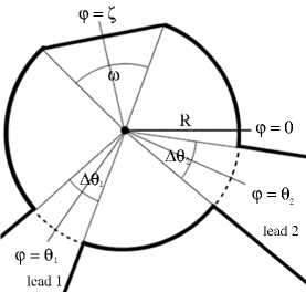
FIG. 1.: Geometry of the scattering system with cavity radius $R$, lead positions at $\theta_{1}$ and $\theta_{2}$, lead opening angles $\Delta\theta_{1}$ and $\Delta\theta_{2}$, cut position at $\zeta$ and cut angle $\omega$.

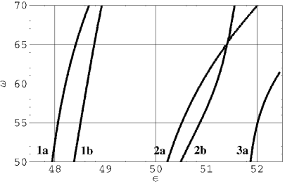
FIG. 2.: Five energy eigenvalues of the closed cut billiard as a function of dimensionless energy $\epsilon$ and cut size $\omega$. From left to right we label them as 1a, 1b, 2a, 2b, and 3a. For $\omega=0^{\circ}$, the states 1a and 1b are degenerate with quantum numbers $(l=3,n=2)$, the states 2a and 2b are degenerate with $(l=6,n=1)$, and 3a is one of a degenerate pair with $(l=1,n=3)$.

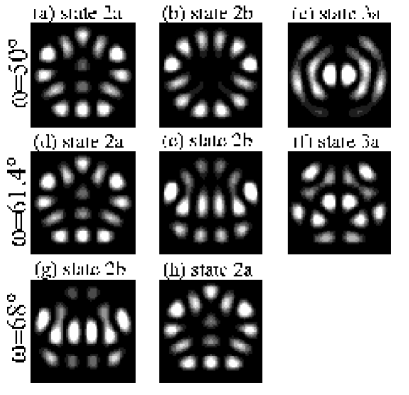
FIG. 3.: Three energy eigenstates corresponding to energy eigenvalues 2a, 2b, and 3a in Fig. 2. The cut is located at $\zeta=270^{\circ}$. The top row has $\omega=50^{\circ}$ and consists of (a) State 2a for $\epsilon=50.2$, (b) State 2b for $\epsilon=50.5$, and (c) State 3a for $\epsilon=51.9$. The middle row has ${\omega}=61.4^{\circ}$ and consists of (d) State 2a for $\epsilon=51.0$, (e) State 2b for $\epsilon=51.3$, and (f) State 3a for $\epsilon=52.4$. The bottom row has $\omega=68^{\circ}$ and consists of (g) State 2b for $\epsilon=51.5$ and (h) State 2a for $\epsilon=51.7$. Note that, from left to right, we show states with increasing energy. This means that 2a and 2b switch position from the middle to the bottom row, as their eigenenergies cross.

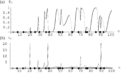
FIG. 4.: (a) Transmission probability and (b) delay time spectra for lead openings $\Delta\theta_{1}=20^{\circ}$, $\Delta\theta_{2}=20^{\circ}$ and lead positions $\theta_{1}=0^{\circ}$ and $\theta_{2}=180^{\circ}$. Eigenvalues of the closed circle are marked by filled (degenerate eigenvalues) and open (non-degenerate eigenvalues) circles.

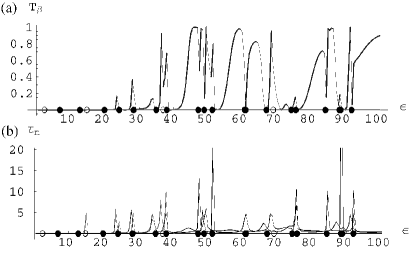
FIG. 5.: (a) Transmission probability and (b) delay time spectra for lead openings $\Delta\theta_{1}=20^{\circ}$, $\Delta\theta_{2}=20^{\circ}$ and lead positions $\theta_{1}=0^{\circ}$ and $\theta_{2}=125^{\circ}$. Eigenvalues of the closed circle are marked by filled (degenerate eigenvalues) and open (non-degenerate eigenvalues) circles.

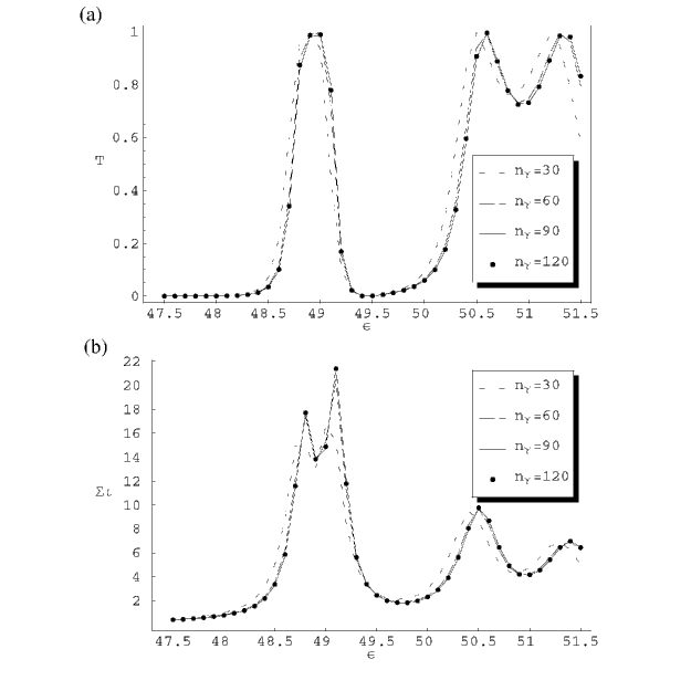
FIG. 6.: (a) Transmission spectra and (b) spectra of the sum of partial delay times in the dimensionless energy interval $47.5{\leq}\epsilon{\leq}52.5$, for cut size $\omega{\leq}80^{\circ}$. The lead openings are $\Delta\theta_{1}=\Delta\theta_{2}=16^{\circ}$. Lead and cut positions are $\theta_{1}=0^{\circ}$, $\theta_{2}=120^{\circ}$, and $\zeta=240^{\circ}$. The results for different values of $n_{\gamma}$ are compared.

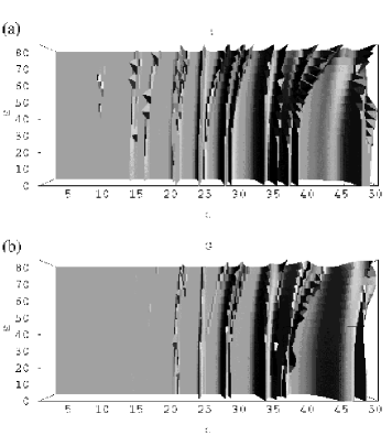
FIG. 7.: (a) Sum of the partial Wigner delay times and (b) conductance for lead opening $\Delta\theta=20^{\circ}$ and varying cut size $\omega$. The leads are centered at $\theta_{1}=0^{\circ}$ and $\theta_{2}=166^{\circ}$, and the cut is centered at $\zeta=225^{\circ}$.

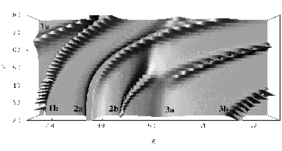
FIG. 8.: Spectrum of the sum of partial delay times for the energy interval $47.5{\leq}\epsilon{\leq}52.5$ and cut size interval $20^{\circ}{\leq}\omega{\leq}80^{\circ}$. The lead openings are $\Delta\theta_{1}=\Delta\theta_{2}=16^{\circ}$. Lead and cut positions are $\theta_{1}=0^{\circ}$, $\theta_{2}=120^{\circ}$, and $\zeta=240^{\circ}$.

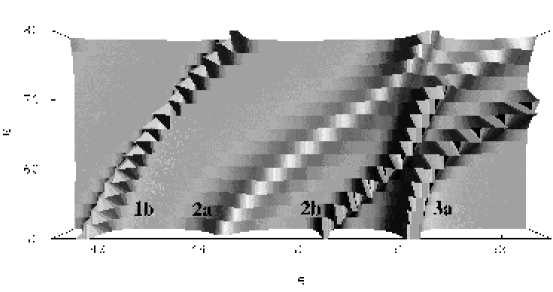
FIG. 9.: Spectrum of the sum of partial delay times for the energy interval $47.5{\leq}\epsilon{\leq}52.5$ and cut size interval $52^{\circ}{\leq}\omega{\leq}80^{\circ}$. The lead openings are $\Delta\theta_{1}=\Delta\theta_{2}=16^{\circ}$. Lead and cut positions are $\theta_{1}=0^{\circ}$, $\theta_{2}=166^{\circ}$, and $\zeta=225^{\circ}$.

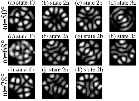
FIG. 10.: Electron probability distribution in the waveguide cavity at the resonance energy for Fano resonances shown in Fig. 9. The lead openings are $\Delta\theta_{1}=\Delta\theta_{2}=16^{\circ}$. Lead and cut positions are $\theta_{1}=0^{\circ}$, $\theta_{2}=166^{\circ}$, and $\zeta=225^{\circ}$. The top row has $\omega=50^{\circ}$ and consists of (a) State 1b for $\epsilon=47.8$, (b) State 2a for $\epsilon=49.2$, (c) State 2b for $\epsilon=50.2$, and (d) State 3a for $\epsilon=51.1$. The middle row has $\omega=68^{\circ}$ and consists of (e) State 1b for $\epsilon=48.5$, (f) State 2a for $\epsilon=50.7$, (g) State 2b for $\epsilon=51.3$, and (h) State 3a for $\epsilon=52.3$. The bottom row has $\omega=78^{\circ}$ and consists of (i) State 1b for $\epsilon=49.2$, (j) State 2a for $\epsilon=50.7$, (k) State 2b for $\epsilon=52.2$.

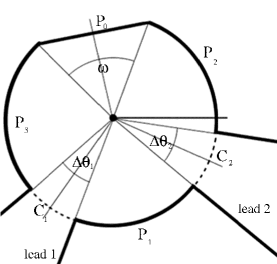
FIG. 11.: Integration contour for the cut-circle waveguide, consisting of $C_{1},C_{2},P_{0},P_{1},P_{2}$, and $P_{3}$.

REFERENCES

- [1] H. U. Baranger, R. A. Jalabert, A. D. Stone, Chaos 3 665 (1993).
- [2] C. Rouvines and U. Smilansky, J. Phys. A 28 77 (1994).
- [3] C. M. Marcus, R. M. Westervelt, P. F. Hopkins, and A. C. Gossard, Chaos 3 643 (1993); A. M. Chang, H. U. Baranger, L. N. Pfeiffer, and K. W. West, Phys. Rev. Lett. 73 2111 (1994); I. H. Chan, R. M. Clarke, C. M. Marcus, K. Campman, and A. C. Gossard, Phys. Rev. Lett. 74 3876 (1995); A. G. Huibers, S. R. Patel, C. M. Marcus, P. W. Brouwer, C. I. Duruoz, and J. S. Harris, Jr., Phys. Rev. Lett. 81 1917 (1998).
- [4] Gursoy B. Akguc and L. E. Reichl, J. Stat. Phys. 98 813 (2000).
- [5] S. Ree and L. E. Reichl, Phys. Rev. B 59, 8163 (1999).
- [6] M. Persson, J. Petterson, B. von Sydow, P. E. Lindelöf, A. Kristensen, and K. F. Berggren, Phys. Rev. B 52, 8921 (1995).
- [7] K. F. Berggren, L. L. Ji, and T. Lundberg, Phys. Rev. B 54, 11612 (1996).
- [8] L. A. Buminovich, Commun. Math. Phys. 65, 295 (1979).
- [9] S. Ree and L. E. Reichl, Phys. Rev. E 60, 1607 (1999).
- [10] T. Timberlake and L. E. Reichl, Phys. Rev. A 59, 2886 (1999).
- [11] C. M. Marcus, R. M. Westervelt, P. F. Hopkins, and A. C. Gossard, Chaos 3, 643 (1993).
- [12] J. von Neumann, E. Wigner, Phys. Z. 30, 467 (1929); English translation in R. Knox, A. Gold, Symmetry in the Solid State (W. A. Benjamin Inc., New York, 1964).
- [13] R. Landauer, Phil. Mag. 21, 863 (1970); R. Landauer, J. Phys. Condens. Matter 1, 8099 (1989); M. Büttiker, Phys. Rev. Lett. 57, 1761 (1986)
- [14] K. Na and L. E. Reichl, J. Stat. Mech. 93, 519 (1998).
- [15] C. Jung and T. Seligman, Phys. Rep. 285, 77 (1997).
- [16] H. R. Frohne, M. J. McLennan, and S. Datta, J. Appl. Phys. 66, 2699 (1989).