Virginia Polytechnic Institute and State University, Blacksburg, VA 24061-0435, USA 33institutetext: Fachbereich Physik, Universität - Gesamthochschule Essen, D-45117 Essen, Germany.
A Lattice Gas Coupled to Two Thermal Reservoirs: Monte Carlo and Field Theoretic Studies
Abstract
We investigate the collective behavior of an Ising lattice gas, driven to non-equilibrium steady states by being coupled to two thermal baths. Monte Carlo methods are applied to a two-dimensional system in which one of the baths is fixed at infinite temperature. Both generic long range correlations in the disordered state and critical poperties near the second order transition are measured. Anisotropic scaling, a key feature near criticality, is used to extract and some critical exponents. On the theoretical front, a continuum theory, in the spirit of Landau-Ginzburg, is presented. Being a renormalizable theory, its predictions can be computed by standard methods of -expansions and found to be consistent with simulation data. In particular, the critical behavior of this system belongs to a universality class which is quite different from the uniformly driven Ising model.
pacs:
64.60.Ht Dynamic critical phenomena and 64.60.Ak Renormalization-group, fractal, and percolation studies of phase transitions and 05.10.Ln Monte Carlo methods and 05.70.Ln Non–equilibrium thermodynamics, irreversible processes.1 Introduction
In recent years, there has been considerable interest in the collective behavior of many body systems which, despite being far from equilibrium, have settled in time-independent steady states. Unlike their equilibrium counterparts, there is no simple Boltzmann factor which provides, in general, the distribution for these non-equilibrium steady states, so that most of the progress to date is made by studying specific cases. One distinguishing feature of these systems is their coupling to more than one reservoir of energy, so that there is a constant “through-flux” of energy. Examples include particles driven by external fields such as gravity or DC electricity, gaining energy from these fields and losing energy thermally to their environment. An important class is driven diffusive systems kls ; DL17 , which were motivated physically by the properties of fast ionic conductors FIC and theoretically by their simplicity. In particular, they are arguably the simplest generalization of the well-known Ising model ising to non-equilibrium conditions. In this paper, we investigate a lattice gas in which particle hopping rates are controlled by two thermal baths, with temperatures and , first introduced in glms . Of course, systems subjected to two (or more) baths are extremely common, from food being cooked on a stove to the earth as a whole. In most cases, temperature gradients (in space or time or both) are present, so that the “steady” states are typically inhomogeneous, controlled by “external” parameters with macroscopic length scales. An excellent example is Rayleigh-Bénard cells, where macroscopic length scales are introduced through gravity as well as temperature gradients. Not surprisingly, large scale properties in such systems can be quite complex, while universal features may be well hidden. In contrast, this two-temperature model is macroscopically homogeneous in both space and time, so that crucial features associated with non-equilibrium steady states are prominently displayed in the foreground.
Of the many large scale (in both space and time) phenomena displayed by this class of non-equilibrium systems, two have received considerable attention. One is the presence of long range correlations at all temperatures above criticality, despite the absence of long range interactions or dynamics (e.g., jumps) at the microscopic level. First revealed in the uniformly driven lattice gas LRC-DDS , they have also been observed in the randomly driven lattice gas LRC-RDDS and the two-temperature models LRC-TT . The other remarkable behavior is associated with the critical point, where significant deviations from the Ising universality class were found marro ; VM ; ktl ; epl ; wang ; antimarro . Here, we focus on the simple two-temperature Ising lattice gas and present an extensive Monte Carlo study, with many results beyond those briefly reported in epl . In this model, particle-hole pairs in the -direction exchange randomly, simulating coupling to a bath with . Exchanges in the -direction do depend on the energy change in a manner consistent with coupling to a reservoir at . As we vary , we observe a second order phase transition, similar to the one found by Onsager Onsager , but located at an approximately 40% higher value. A careful study of the two-point correlations in the disordered phase verifies the long-range nature () to a much better extent than before LRC-TT . These long-range correlations are “generic” glms ; GG and can be easily understood zhls through a Langevin equation for a continuum field, which is simply a non-equilibrium version of time-dependent Landau-Ginzburg theory. Based on this theory, a renormalization group (RG) analysis can be applied to extract the critical behavior. Reported briefly in the past SZ-prl ; S-epl , the details of such an analysis are given here. Similar to the uniformly driven lattice gas, momenta in the - and -directions scale with different power laws. Unlike the uniformly driven lattice gas, where the powers differ by a factor of three (in two dimensions), the difference here is much closer to the “mean-field” value of two. Relying on these results, we carried out extensive simulations using a series of rectangular samples (), so as to simplify the finite size scaling analysis. We measured a cumulant ratio, the “magnetization”, the “specific heat” and “energy” fluctuations. A consistent picture emerges, in general agreement with theoretical predictions. In contrast, using the customary square samples (), no consistent set of parameters can be found to collapse the data. Undoubtedly, a new scaling variable is playing a dominant role here. Our conclusion is that anisotropic scaling is crucial and that the simulations support the field theoretic renormalization group analysis of this system.
The paper is organized as follows. In the next section, the lattice model and its continuum partner will be described. Simulation methods and results, as well as comparisons with the theoretical predictions, may be found in Section 3. For completeness, we present details of the field theoretic renormalization group analysis (Section 4). A concluding section is devoted to a summary and an outlook.
2 The Discrete Model and A Continuum Theory
2.1 A Two Temperature Lattice Gas
The constituents of our model are identical to the two-dimensional Ising lattice gas ising ; YangLee . On a square lattice with fully periodic boundary conditions, the sites may be empty or occupied by a single particle, so that a configuration, , is completely specified by the set of occupation numbers , with each being or . In general, our system will be rectangular, i.e.,
with typically. The particles interact with nearest neighbor attraction, so that, in the Hamiltonian
| (1) |
is positive. We choose here so that the effective part of in the spin language is just , since . To simulate diffusing particles, we will allow only particle hops to empty nearest neighbor sites, a dynamics corresponding to Kawasaki spin exchange Kawasaki . Thus, the total particle number is conserved and, in all cases studies here, fixed to be , where
| (2) |
Such a half-filled lattice is equivalent to a spin system with zero total magnetization (), so that the critical point can be accessed.
If this system is in contact with a single thermal bath at temperature , then the probability for finding it in any configuration is given by the Boltzmann factor
| (3) |
and many of its properties are well known McCoyWu . For temperatures above the Onsager Onsager value, , the system is in a homogeneous, disordered state. Particle-particle correlations decay exponentially, governed by a finite correlation length . As , while correlations decay with a power law. Thermodynamic quantities develop singularities as a function of various parameters. Due to the constraint , the ordered state for is inhomogeneous, consisting of a particle-rich (mainly ) region co-existing with a hole-rich one (mainly ). Given the boundary conditions, each of these regions is a single strip, of width , spanning the lattice along (where is the longer dimension, etc.). In this manner, the interfacial energy is minimized. Thus, for example, states with vertical strips will dominate in a system with . Finally, the average within one of these regions will be, in the thermodynamic limit, the spontaneous magnetization: .
Our interest in this model lies in its behavior when placed in contact with two baths, at different temperatures. In general, we can expect energy to flow through our system, from one bath to another. In the limit that the baths are infinitely larger than the lattice gas, this energy flux will settle down to a constant (on the average) and our system reaches a non-equilibrium time-independent state. However, unlike Eqn (3) above, the steady state probability distribution, is not known in general. Indeed, is expected to depend on the details of the dynamics, namely, how our system is coupled to the two baths. Nevertheless, within a class of models, we believe that there are many universal properties which do not depend on such details. Here, we will focus on a particular model, deferring a discussion of the universality class until Section 4.
To completely specify our model, we list the rules of time evolution:
-
•
choose a random nearest neighbor particle-hole pair
-
•
if the pair lies along the -direction, exchange them
-
•
if the pair lies along the -direction, exchange them with probability , where is the energy change due to the exchange.
Note that the second rule can be replaced by one similar to the third, with , the temperature of the second bath. Here, we have further simplified the model by setting Of course, this model may be tied “continuously” to the equilibrium case by lowering down to .
In our Monte Carlo simulation, a random pair is first chosen. If this is a particle-hole pair, the rules above apply; otherwise, another pair will be randomly chosen. A Monte Carlo step (MCS) is defined by attempts. Starting from, typically, a random initial configuration, the system is evolved for up to MCS. Allowing the first MCS for the system to come to steady state, we measure various quantities every - MCS. The results quoted in the next section are obtained by averaging these measurements.
As will be discussed in more detail, the second order phase transition is found to survive. However, the critical temperature is raised by approximately ! In addition, the two-particle correlation function develops power law decays at all temperatures in the disordered phase, while the critical properties are modified from the equilibrium Ising class WilsonFisher . To understand such collective behavior in the long-time and large-scale limit, we often rely on continuum descriptions. This is the topic of the next subsection.
2.2 Formulation of a Langevin Equation
In this subsection, we formulate a continuum approach, based on field theory. For the convenience of readers who may not be familiar with this approach, we first summarize the well-established steps for the Ising model in equilibrium. In that case, a series of continuum theories yield better and deeper understanding of its properties. The simplest continuum description starts with Landau’s macroscopic free energy function for the magnetization
which focuses only on spatially homogeneous features. To capture spatial inhomogeneities and thermal fluctuations, we rely on the “mesoscopic” Landau-Ginzburg Hamiltonian for a magnetization which is a coarse-grained version of from the lattice model. Furthermore, from renormalization group studies, we learned that it is important to formulate such theories in general dimension WilsonFisher (even though our simulations are restricted to ). Thus, we write
| (4) |
Far from the critical point, which is modeled by vanishing here, good agreement with data can be gleaned from by inserting Eqn (4) into Eqn (3), i.e., , and relying on simple approximation schemes in subsequent computations. Near the phase transition, however, more powerful renormalization group techniques RG are needed, providing excellent predictions of long-wavelength properties, such as critical behavior. Further, these approaches can be generalized to dynamic phenomena ZJ ; DF near equilibrium, starting with a Langevin equation for .
For later reference, we briefly review this procedure for the Ising model, in the presence of a conservation law on the total magnetization . Then, the Langevin equation takes the form of a continuity equation:
| (5) |
The form of the current is postulated, guided by the symmetries and key physical features of the microscopic rates. It typically consists of a deterministic term, capturing the thermodynamic forces acting on , and a Gaussian noise term which reflects the effect of thermal fluctuations. For the Ising model, the deterministic part ensures that relaxes towards configurations of lower energy. Moreover, must be chosen such that the known equilibrium distribution, , controls the static properties of . This constraint forces the Langevin equation to satisfy the fluctuation-dissipation theorem (FDT) FDT . Let us briefly recall the resulting structure. The most general form of the Langevin equation is
| (6) |
Here, is a functional of and its derivatives, constructed on physical grounds in the spirit of a Landau expansion. It reflects the deterministic part of the dynamics. denotes the noise term, with correlations
| (7) |
is just a positive constant which measures the strength of the correlations. More importantly, the noise “matrix” carries information about conservation laws or internal symmetries which are obeyed by the dynamics. For our purposes, it is sufficient to consider only a scalar order parameter and noise matrices which do not depend on . (More general cases are discussed in, e.g., risken and hkj .) Given this basic form, a steady-state solution for the configurational probability is easily found risken provided is “Hamiltonian”, i.e., if it can be written as acting on the functional derivative of an appropriate Hamiltonian :
| (8) |
In this case, the steady state is simply the equilibrium distribution, , irrespective of the choice of . We will refer to such a dynamics, in an operational sense DL17 , as “FDT-satisfying”. Note that the “noise strength,” , plays the role of a temperature here. Since it just sets the scale for the energy, it may be absorbed into the definition of . In the Ising case, the microscopic dynamics is isotropic (at least near the critical point) and order-parameter conserving, so that . Our preceding discussion suggests the equation of motion
| (9) |
with
| (10) |
The current is therefore , where the second term is the noisy part, related to simply by . The coefficient sets the time scale. In fact, symmetry considerations alone would have forced us into this form, even without invoking the FDT: the deterministic part of (9), just contains the leading terms of a general Landau expansion, in powers of and which are consistent with all symmetries of the Ising model.
This Langevin equation, known as Model B HH , describes the critical dynamics of a conserved scalar order parameter. The time-independent, or static, aspects of its critical behavior are controlled by and fall into the equilibrium Ising class. In addition, one obtains time dependent properties as well, such as the dynamic critical exponent and the scaling behavior of dynamic correlation and response functions. These are characteristic for the Model B class. We note, for later reference, that the critical parameter, , now plays the role of a diffusion coefficient: As drops below , becomes negative indicating that “antidiffusion”, i.e., phase segregation, occurs.
Following these lines, we formulate a continuum theory for our non-equilibrium Ising lattice gas. Once again, we begin with a continuity equation for , so that the conservation law is guaranteed. Before writing an expression for the current, however, it is paramount that we should summarize the symmetries of our microscopic theory. Like the equilibrium Ising model, it exhibits full translation and reflection invariance, as well as the characteristic Ising “up-down” symmetry. However, in contrast to its equilibrium counterpart, even near criticality we can no longer expect full rotational symmetry, since distinct temperatures, , control exchanges along different directions . In the simulations, and while . Clearly, we enjoy some freedom here in extending this model to general dimensions: in principle, we could imagine couplings to different temperature baths, with temperatures . However, the most interesting and fundamental case remains that of just two baths, with and . In other words, we select a one-dimensional subspace to be coupled to the higher temperature ( in simulations). The full rotational symmetry, , of the Ising model is obviously reduced to an symmetry in the remaining dimensions. We will refer to the subspace associated with the higher temperature as “parallel” (e.g., ) and the complementary subspace as “transverse” (). In the section on field theoretic studies, we will return briefly to the general case, in order to show that all nontrivial features are indeed captured by the simpler two-temperature theory.
Given the restricted rotational invariance of our model, we can no longer expect the same Landau expansion for the currents in the parallel and the transverse subspaces. In particular, all operators should be split into parallel () and transverse () parts, accompanied by different coefficients. Note, however, that invariance under reflections guarantees that gradients still appear in pairs: or . Thus, “splits” into , becomes , and turns into . By appropriate rescaling of both parallel and transverse lengths, and can be set to unity. Thus, we can write the most general Landau expansion which still respects all symmetries of the microscopic theory as
| (11) | |||||
where, for later convenience, we have written () for (). Turning to the noise, while keeping it Gaussian, we should expect different variances in the two subspaces. Hence,
| (12) |
where the ’s represent the noise strengths. Since the transverse subspace is still fully isotropic, we have . Generically, however, we should expect . Clearly, the noise terms could also have been expressed via , with correlations . Higher derivatives or powers of the order parameter which have been neglected above are expected to be small above the critical point. Near , they will be irrelevant, in the renormalization group sense, as we will see in Section 4.2.1.
This Langevin equation forms the basis of our theoretical analysis. Since the isotropic diffusion term in Eqn (9), , has been modified to , with two different “diffusion” coefficients for the parallel and transverse subspaces, a serious question arises. Should we expect both, or just one, of these to vanish as approaches criticality? For the equilibrium system, we recall that the lowering of is a consequence of the presence of interparticle interactions which slow (or even reverse) the decay of density gradients, as decreases. In the two-temperature model, the parallel subspace is held at a higher temperature than the transverse one, suggesting that density gradients should decay much faster in the parallel directions. Thus, we anticipate that, generically, so that criticality, in particular, is marked by vanishing at positive . This is borne out by the structure of typical ordered configurations, namely, single strips aligned with the parallel direction, indicating that “antidiffusion”, i.e., , dominates in the transverse directions below .
The inequality satisfied by the diffusion coefficients is obviously crucial for the correct description of criticality. Otherwise, it is fortunate that the detailed dependence of the parameters in Eqns (11) and (12) on the microscopic , , and , is not important. In the disordered phase, Eqns (11) and (12) can be simplified even further, by truncating the Landau expansion after linear terms, considering, in effect, a purely Gaussian theory.
To conclude this section, let us check whether Eqns (11,12) satisfy the FDT. Comparing our noise correlations with Eqn (7), we read off . It is straightforward to see that it is impossible to recast the right hand side of Eqn (11) in the Hamiltonian form of Eqn (8). We conclude that our continuum theory for the two-temperature model generically violates the FDT. However, in Section 4 we will show that the critical properties are controlled by a fixed point theory which is associated with, surprisingly, a system (not Ising) in equilibrium S-epl . The implications are that FDT is restored in the critical region, for the leading singular parts of thermodynamic quantities.
3 Simulation Results
This section will be devoted to the main results from Monte Carlo simulations on the two dimension model specified in Section 2.1. In the first sub-section, we study the two-point correlations in the disordered phase, showing convincing evidence for power law decays in configuration space. In the second part, extensive investigations of the critical properties will be presented. We will use subscripts and for the “parallel” () and “transverse” () directions, respectively. In the remainder of this article, will be quoted in units of the Onsager value .
3.1 Two-point Correlations Far Above Criticality
For an Ising model in equilibrium, regardless of the dynamical aspects of the system, two-point correlations
display power law decay only at the critical point. However, for a system driven into a steady state under non-equilibrium conditions, the asymptotic behavior of will depend on the dynamics. In particular, for our model at any above the critical point, decays as , where . Of course, the associated amplitude must be direction dependent, so that the integral over space is not divergent. In general, a simple rescaling of one co-ordinate (say, ) will bring it to the same form as an electrostatic potential of a quadrupole (in ) glms ; LRC-TT , so that there are long range positive/negative correlations in the longitudinal/transverse direction, i.e.,
| (13) |
and and are positive amplitudes depending on and . Had we used a finite , both would depend on the difference as well, in a manner that vanishes as . The presence of these amplitudes can be traced to FDT violation in these systems, as we will see in Section 4.1. Here, we provide some details of how this power law behavior can be observed directly in , as well as the simpler, “indirect” method using the Fourier transform of
We begin with the simpler way, i.e., by measuring the structure factor
and seeking a discontinuity singularity zhls at the origin . Unlike the Ornstein-Zernike form for the equilibrium Ising model, where
with being the static susceptibility, the limit depends on the direction of as it approaches the origin glms ; zhls . In particular, the maximum range is embodied in, say,
| (14) |
Another convenient way to express such a discontinuity is
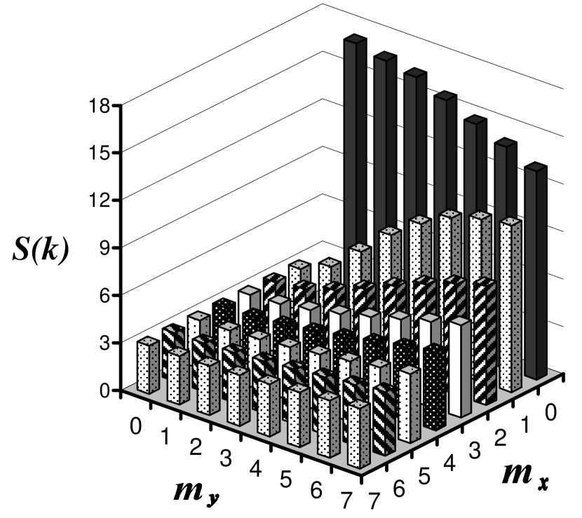
Now, for a finite system, the wave-vectors are discrete, being with integer . Further, our system is set at , so that . Thus, through measuring at the two lowest wave-vectors:
in a series of systems with various and , the discontinuity singularity in (14) can be estimated by extrapolation. Here, we are content to display the presence of such a discontinuity, as in the first Monte Carlo study of driven systems kls .
In Fig. 3.1, we show for the case at . For this plot, we made measurements every MCS on 5-10 runs, each up to MCS. Note the sizable difference between and . By contrast, for the equilibrium case, these two quantities would be the same, within statistical errors.

Parenthetically, let us point out that, for the series, a multitude of long runs are crucial for minimizing the scatter in the data. This “difficulty” may be traced to another manifestation of long range correlations like Eqn (13), namely, the presence of strips along which are anti-correlated in . This property favors slow decays of strips with a range of widths, so that short runs may find only configurations “locked in” particular regions of phase space. We believe that this phenomenon is intimately tied to the metastability of “multistrip configurations” first reported in VM .
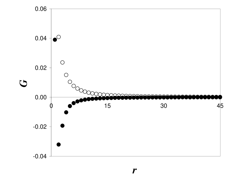
Though the discontinuity in is the easiest way to deduce the presence of a power law decay, it is naturally more satisfying to observe the evidence directly. Indeed, in the early studies LRC-DDS ; LRC-TT , is measured along the two axes and vs. is plotted. However, the data used there to support the behavior are susceptible to criticisms. Typically, a straight line is drawn through less than 10 scattered points, even though sizes up to were used. In the study on the two-temperature model LRC-TT , low statistics (K MCS) further limits the reliability. To remedy this situation, we carried out a more careful study, measuring every MCS on 5-10 runs, each up to MCS, on a system at . In Fig. 3.2, we present and vs. or
Apart from finding a more convincing evidence of the decay, we discovered a non-trivial finite size effect, which must be taken into account before a log-log plot can be exploited. Due to the conservation law , we have , so that the asymptotic behavior of the two-point correlation in a finite system is not zero. Indeed, for the totally disordered state (), we must have . As a result, for high , the power law tail (13) can be easily overwhelmed by negative contributions. In practice, the precise values of these corrections (for finite ) are not known and represent the only parameters in the fitting procedure. The result reveals excellent decays. In Figs. 3.3 and 3.4, dashed lines of slope are included simply for the sake of comparison. From these plots, we conclude that the behaviors (13) are well established.

3.2 Critical Properties
As is lowered toward a critical value, , correlations build up and the system is expected to undergo a continuous transition to an ordered state, characterized by phase segregation. Unlike in the equilibrium Ising case, this segregation occurs only along the -direction, a phenomenon undoubtedly related to the anisotropic long-range correlation above . Another manifestation of this type of ordering is that only diverges (as for ), while remains for all temperatures. The consequences of this behavior are quite serious. Further, without some theoretical elucidations, the pitfalls awaiting finite size analysis in computer simulation studies are well hidden. As an example, in contrast to the equilibrium case, the use of samples (with a series of ’s) will not lead to consistent collapse of data (Section 3.4). Instead, due to the conserved dynamics and FDT violation, lengths/momenta in the two directions scale with different exponents SZ-prl , as will be shown in detail below (Section 4.1). Thus, we resort to the method of “strong anisotropic scaling”ktl ; wang , i.e., using a series of rectangular samples with fixed and non-trivial
Before delving into the details of the results, let us provide an “appetizer” for the origins of a non-zero , from “mean field theory”. To describe this transition in the equilibrium case, Landau let (in Eqn 4) go through zero. As a result, the leading relaxation term in (4) vanishes, regardless of the noise “matrix” . In particular, for (9) both diffusion coefficients vanish at the same (critical) temperature. However, without the constraint of FDT, it is not necessary that both vanish at one . Indeed, to describe phase segregation into horizontal strips (along with being ), it is natural to let only the transverse diffusion coefficient, , in (11), vanish. As a result, the leading restoration terms become and , which translate into
in the language relevant for our simulations. Since the effects of these are supposedly comparable in the critical region, the implication is
| (15) |
But, the lowest wavevectors available to our finite system are and . To insure that both types of fluctuations are comparable in the critical region, we must choose Thus, we arrive at the “mean field” result
| (16) |
As will be shown (Section 4.2), corrections to this result are expected to be small, even in (unlike the uniformly driven lattice gas, where ). Thus, for convenience, we simply used systems with , namely, , , , , and . To have some confidence that is indeed small and positive, we also carried out runs with and . All results are entirely consistent within statistical errors, in that a good quality of data collapse is observed. By contrast, the use of square samples does not lead to consistent data collapse (Section 3.2.3), signaling the presence of another scaling variable:
| (17) |
Finally, let us remark on possible choices for order parameters. Due to the conservation law, is fixed at zero and cannot serve as the order parameter. Instead, in the seminal work on driven systems kls and several subsequent studies marro , a quantity was used which is sensitive to ordering into horizontal strips rather than vertical ones:
| (18) |
However, (18) is likely to overestimate the segregation into two macroscopic phases ktl ; wang . For example, it cannot distinguish single strip configurations from multiple strip ones, as long as the latter are all horizontal. Further, since it is a sum of over all ’s (along both axes in space) up to the ultraviolet cut-off, its scaling properties are quite nebulous. Therefore, we decided upon the structure factor being the clearest measure of the spontaneous symmetry breaking, as our order parameter ktl . Configurations with multiple strips contribute little to this quantity. Also, as a correlation function associated with the smallest possible wavevector, there is little doubt on how to compare simulation data with field theoretic predictions.
3.2.1 Crossing of a Cumulant Ratio, Data Collapse and the Exponent
For the equilibrium Ising model, Binder Binder introduced a convenient ratio , which varies monotonically between and as ranges in , regardless of In the thermodynamic limit, it should be a simple step function, with the step occurring at the critical temperature. For finite ’s, curves should cross at temperatures approaching Furthermore, the value at the crossing is predicted to be universal Binder , so that this method has been the favorite for the first determination of the critical temperature. For our model, is clearly futile, since it is identically zero. Instead, we must consider the first non-zero wavenumber in the Fourier transform:
Note that we chose as our order parameter. The equivalent cumulant ratio here is ktl ; wang
| (19) |
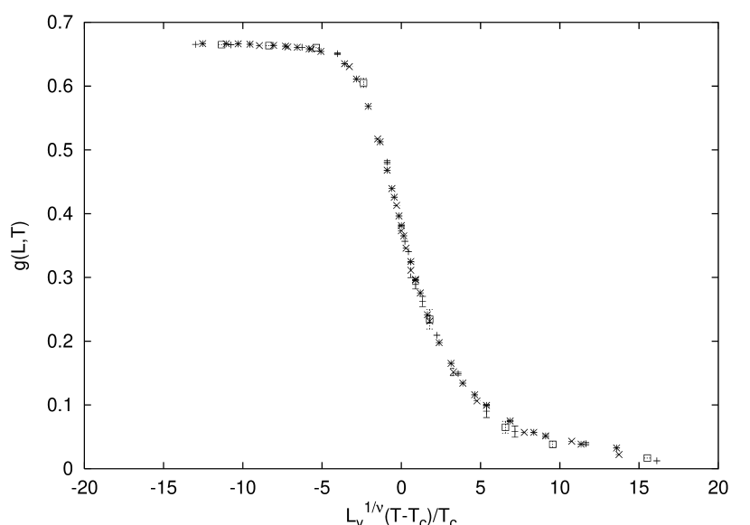
In this definition, the dependence on is suppressed, since we have used only sizes which correspond to fixed . Also, due to , it is more convenient to have as the first term, so that . At the opposite end, , so that is precisely the Heaviside function: . In the inset of Fig. 3.5, we plot the ratio against for the system sizes chosen. Within the errors of our simulations, the crossing occurs at

More importantly, when plotted against the scaling variable
| (20) |
all curves may be collapsed into a single one (Fig. 3.5), with
| (21) |
and
| (22) |
Note that we have tested the effects of having slightly less than as well. We are encouraged by the data associated with these cases ( and ) also lying within the typical scatter of the “universal” curve. Thus, it is not crucial that we keep careful account of the possible presence of a small . The value for the exponent is entirely consistent with the results of renormalization group calculations (Section 4.2.3).
Finally, we emphasize that a general scaling ansatz for should be of the form . Thus, the use of square samples would have introduced the added complication of a varying . However, if were to enter as an additional power, then data collapse can still be achieved, but with another value for . We will return to this topic in Section 3.2.3.
3.2.2 Scaling Plot of and the Exponent
From scaling arguments, the other independent exponent may be chosen as . By definition, it is the anomalous dimension associated with the structure factor at criticality in the limit of small . In models with “strong anisotropy” such as ours, we must be more careful and define it to be the anomalous dimension in . (See Section 4.2.2 below for other -like exponents.) For that reason, serves conveniently in a finite size scaling analysis to extract . In practice, it is more convenient to use ktl
which is normalized to unity at . Thus, the presence of scaling is signaled by being a function of alone. Of course, there are generally two branches, associated with ’s above/below criticality. For , we may define in the usual way, via in the thermodynamic limit. In other words, should be proportional to . Using the definition of , we obtain the usual scaling relation . Meanwhile, for , plays the important role of for non-conserved systems and serves to probe , the order parameter exponent. So, should be a function of alone, leading to another scaling relation: . Thus, data collapse in a single scaling plot, for both above and below , is a good test of the hyperscaling relation:
| (23) |
As will be shown below, field theory predicts , so that its validity can be tested by plotting against and checking for data collapse. Further consistency can be verified by extracting the exponents and from the two branches and checking if they correspond to and , respectively.

Fig. 3.6 shows a log-log plot of the best data collapse of the two branches, using (21) for and (22) for . To guide the eye, and to show consistency, we have inserted lines with the expected slopes. From this graph (and others with varying values of ) we estimate the value
| (24) |
and conclude that a consistent set of exponents exists, including
The smaller samples deviate from the collapse as the temperature rises. This deviation can probably be traced to the following. For small system sizes, larger temperature ranges are needed to accumulate data for the scaling plot, corresponding to ’s further outside the critical region.
3.2.3 Data from Square Samples
In order to test the importance of “strong anisotropic scaling,” we have also performed simulations using square samples from to . With data from such runs, it is possible to achieve reasonably good collapse of , using and (Fig. 3.7). However, with these values for and , the best “collapse” we can achieve for is shown in Fig. 3.8, with . Better collapse of these data can be accomplished, but only by using values of and different from those in Fig. 3.7, or at the expense of a large, negative value of ! We believe that the lack of good data collapse (with a consistent set of values for the critical temperature and exponents) is a strong indication that another scaling variable is playing a dominant role. In this case, it would be . If we use the mean-field value for , then this variable ranges over a factor of , for the set of data presented. Such a large variation should be enough to explain the significant scatter in Fig. 3.8.

In the literature, it has been claimed that consistent data collapse can be achieved using square samples marro . However, we believe that, by using a different order parameter (Eqn (18)), these authors may be probing a different “phase.” In connection with the uniformly driven lattice gas, the possible existence of such a “new” phase has been conjectured recently stringy and may resolve the differences observed here. Further investigations are clearly necessary to clarify these issues.
3.2.4 Fluctuations and Specific Heat
For an Ising model in thermal equilibrium, both the free energy and the internal energy, , are well defined and useful concepts. For non-equilibrium systems in steady state, the concept of free energy becomes less clear, especially in our case of having thermal reservoirs at two different temperatures. Nevertheless, we may continue to regard as an internal energy, associated with the interparticle interactions. Furthermore, since anisotropy is expected, we may define the “longitudinal” and “transverse” parts of this energy, by and respectively, where
and
| (25) |
Needless to say, these are nothing but the energies stored in the broken bonds in the two directions.
As in equilibrium, the internal energy is a function of and we may define its response to changes in as the heat capacity
Similarly, its fluctuations can be measured. To emphasize the similarities and differences between our system and one in equilibrium, we consider
Replacing in these expressions by and , we can define similar quantities: , etc. Of course, had we used , we would have , etc. Thus, measurements of all these quantities will provide not only a specific-heat-like exponent , but also the degree of FDT-violation.

We are able to compile reasonably good statistics on the fluctuations (’s). For the critical region, the best data are associated with , the fluctuations in the “transverse” part of the energy (Fig. 3.9). By contrast, due to the positive long range correlations, there are fewer broken “longitudinal” bonds, which may be the reason behind the lower quality of the data for . To study scaling properties, we consider first the positions of the peaks, In Fig. 3.10 (inset), we show a log-log plot of vs. , along with a line of slope of , so that we have a consistent estimate for . On the other hand, a similar plot for the heights of the peaks (Fig. 3.10) leads us to . This value of is also entirely consistent with the scaling relation predicted from field theory (Section 4.2.3), i.e., . Unfortunately, scaling plots for do not exhibit data collapse of the same quality as those for and . We believe that better statistics would remedy this situation. Similarly, the data for energy are not precise enough for estimates of the heat capacities (’s). Nevertheless, we may conclude from these observations that the qualitative features of the ’s are the same as the ’s. In particular, a log-log plot of the heights of the maxima vs. provides us with a similar . However, it is not surprising that the numerical values of the ’s are quite distinct from those for the fluctuations, since FDT is clearly violated.


We end this section with a brief comment on energy fluxes. Since our system is coupled to two temperature baths, we expect that there would be a steady flow of energy through our system, from the bath with to the one with To be specific, with each spin-exchange update, we can track whether it is associated with an -bond or a -bond. Respectively, the energy change resulting from these exchanges would be determined by and We have verified that, in the steady state, the average energy change associated with an -bond spin-exchange is positive. Indeed, far from being just fluctuations, the average change in a MCS, which we denote by , is a few percent of , for all the sizes we investigated. Of course, being in steady state, the average change associated with -bond exchanges is of the same magnitude, but negative: . In other words, the energy flux through the system, , is an extensive quantity. By contrast, for an equilibrium system, the flux is fluctuating around zero, at the order of . Similar differences have been observed in uniformly driven diffusive systems CCP99 . Qualitatively, this flux rises with temperature until about the critical point. Thereafter, it appears relatively constant (Fig. 3.11). A quantitative study of this flux, which lies outside the scope of this paper, would undoubtedly yield rich information about an important non-equilibrium characteristic of this system.
4 Field Theoretic Studies
Exact solutions for many-particle systems far away from thermal equilibrium are restricted mostly to one-dimensional cases DL19 with excluded volume interactions alone. Thus, progress for higher-dimensional models relies entirely on mesoscopic continuum theories, such as the Langevin equation for our two-temperature model. While these field theories cannot be rigorously derived from the microscopic dynamics, many of their key ingredients and predictions are easily tested by Monte Carlo simulations. Considerable confidence in these theories can therefore be established before they are used to predict less easily measurable quantities. In the following, we will outline how some of the simulations results of the preceding sections are reflected in our continuum theory. We begin with the disordered phase, before turning to fully developed critical behavior.
4.1 Long-Range Correlations
Well above , typical configurations are nearly homogeneous, and fluctuations of the local magnetization away from zero are very small. It is therefore reasonable to neglect fourth-order gradient terms as well as higher powers of in our Langevin equation. The resulting theory, for the equilibrium Ising model, is completely analytic for all . In contrast, for our far-from-equilibrium system, even the disordered phase already exhibits nontrivial singularities. In the following, we will discuss how these manifest themselves in our continuum theory.
We begin with the simplified version of Eqns (11,12) which is fully appropriate for the disordered phase:
| (26) |
The noise correlations are given by
| (27) |
Since Eqn (26) is linear, it is easily solved via a Fourier transform to momentum and frequency space. With , where , we find
| (28) |
The corrections in the denominator are a reminder of the neglected fourth-order derivatives. Arbitrary correlation functions follow from (28) by averaging appropriate products of over the Gaussian distribution of the noise.
The most remarkable property of the disordered phase is the presence of power-law correlations, even well above . In the equal-time structure factor, being the Fourier transform of the correlation function, these should be reflected as an anomaly near the origin. Starting from the full dynamic structure factor, defined via , its Fourier transform back into the time domain, , is easily found:
| (29) | |||||
The subscript reminds us that we are considering a purely Gaussian theory. Setting yields the equal-time structure factor, :
| (30) |
In contrast to what one might have expected naively, (30) is not a simple anisotropic generalization, such as , of the usual isotropic Ornstein-Zernike structure factor for the equilibrium Ising model. The key difference resides in the discontinuity singularity exhibited by (30). Defining
we find that both and its isotropic version lead to , indicating that such an anisotropy is too weak to affect the long-wavelength limit. In stark contrast, (30) results in , since the value of at the origin depends on the angle under which vanishes!
At a more fundamental level, this discontinuity singularity is a direct consequence of the violation of the FDT. For linear theories such as ours, the FDT demands that the matrices of noise correlations, , and of diffusion coefficients, , should be proportional to one another. Thus, if the FDT were to hold, the general form (30) would be immediately reduced to . This is the case for, e.g., an Ising model with anisotropic interactions. For our two-temperature model, however, there is no such constraint, so that generically . At criticality, the FDT is maximally violated, i.e., diverges as .
One consequence of such a singularity in is that its Fourier transform, the two-point correlation function , becomes long-ranged, decaying as at large distances. The amplitude, in addition to being proportional to , has a dipolar angular dependence, resulting in positive and negative , in agreement with our data. Of course, our continuum theory presupposes an infinite system, so that no finite size corrections appear here. Moreover, the dipolar character combined with the corrections ensures that an appropriate angular average of is again exponentially cut off DL17 . However, the divergence of at criticality indicates a crossover to a different behavior, which will be the subject of the next section.
To conclude, we note that the Ising “up-down” symmetry of our model ensures that all three-point functions vanish identically above and at criticality. This feature clearly distinguishes our model from the uniformly driven system where such correlations are generically nonzero and can even be singular at the origin, along selected directions 3pf .
4.2 Critical Properties and the Nontrivial Fixed Point
As the temperature approaches , the local magnetization begins to develop large fluctuations, both in absolute value and in gradients. This signals the breakdown of the linear theory, Eqns (26,27), as a valid description of the disordered phase. We should therefore return to the full Langevin equation, Eqns (11) and (12). Our first task is to identify all couplings relevant for critical properties, i.e., retaining non-zero values at the fixed point of the renormalization group. We will see that simple dimensional analysis alone can already exhibit some of the key differences between our two-temperature system and its equilibrium counterpart, Model B. Most remarkably, the fixed point theory restores the FDT, but with respect to a different Hamiltonian. We define a set of critical exponents and perform a scaling analysis for our model, by anticipating the scaling forms for a few key quantities. Finally, we provide the technical foundation for this scaling analysis, in the form of an explicit renormalization group calculation, up to and including two-loop order S-epl .
4.2.1 The Fixed Point Theory and FDT Restoration.
In the continuum theory, (11,12), criticality is marked by the vanishing of the transverse diffusion coefficient, , while its parallel counterpart remains positive. Reconsidering our Landau expansion in powers of gradients, we clearly need the term to limit fluctuations with large transverse gradients, since cannot serve this purpose near . In contrast, fluctuations with large parallel gradients are still controlled by , so that the higher order term, , is not needed and will be neglected. As a result, the two leading linear terms in the Langevin equation, near criticality, are and . Introducing a characteristic momentum scale for transverse critical fluctuations, , we conclude, on the basis of simple dimensional analysis, that parallel wave vectors scale as . In the long-wavelength limit () which is the focus of our study, parallel gradients are therefore less relevant than transverse ones: may be neglected in favor of , and transverse noise correlations dominate parallel ones. Similarly, the mixed term is irrelevant compared to . Collecting so far, we arrive at a reduced Langevin equation, containing relevant terms only:
| (31) | |||||
Here, the noise has been restricted to the transverse subspace, with correlations
| (32) |
This equation forms the starting point for the analysis of universal critical properties. Continuing the dimensional analysis, we find that , characteristic for a conserved order parameter. Care must be exercised with the scaling of the spatial volume. For example, , since parallel lengths generate an extra factor . By construction, both and are of order . In fact, the latter is a trivial coefficient which will be rescaled to in the following. The role of is more intriguing and will be discussed in Section 4.2.3. It is now easy to obtain so that the order parameter itself scales as . The upper critical dimension of our model is since . Since all irrelevant couplings have been neglected, we refer to Eqns (31,32), somewhat loosely, as the fixed point theory. Strictly speaking, we should set also, since the naive scaling indicates that zero is the fixed point value of the transverse diffusion coefficient.
It is instructive to define , where is the dimension of the parallel subspace. In the spirit of the more general models alluded to in Section 2.2, may be considered a model parameter. Of course, we require , for a transverse subspace to exist. Then, the magnetization scales as and , whence . In this form, the similarity to Model B scaling, where , is quite apparent. However, we emphasize that the physical upper critical dimension is , below the Ising model value 4. This already indicates that the two-temperature model falls outside the Ising universality class. Clearly, the only “interesting” case is : then, nontrivial exponents are expected in two dimensions, as borne out by our Monte Carlo simulations. In contrast, the choice results in an upper critical dimension of , for a model that is defined only in dimensions. As a result, only mean-field exponents should be observable in this case.
Returning to Eqns (31,32), we observe an intriguing consequence of neglecting irrelevant terms: the reduced Langevin equation for the near-critical theory obeys the FDT. Defining , and noting that is a positive definite symmetric operator, we can rewrite our Langevin equation as follows:
| (33) |
with a Hamiltonian that is most easily expressed in momentum space:
| (34) | |||||
Since the only relevant contribution to the noise acts in the transverse subspace, its correlations are simply
| (35) |
This structure leads to several important consequences. First of all, near criticality, the static properties of the system are in fact equilibrium-like, being controlled by the distribution . Interestingly, even though our microscopic dynamics is purely local, effective long-range interactions are generated at the mesoscopic level. These are dipolar in nature, as reflected by the static Gaussian propagator
| (36) |
In fact, it is helpful to recall the Hamiltonian for uniaxial ferromagnets with dipolar interactions dipolar . Assuming that the spins are aligned with the parallel direction and located at and , the dipolar interaction takes the form , with . A Fourier transform to momentum space yields . Including the exchange interaction, we obtain the propagator for uniaxial dipolar ferromagnets, , where marks the critical point and is a constant. At first sight, the -dependences of these propagators, and , are obviously not identical. However, closer examination reveals that the difference resides in irrelevant terms alone (e.g., , in a sum with )! Of course, the nonlinear term, in both cases, is just the usual interaction. Thus, we conclude that the leading static critical singularities of our two-temperature model fall into the universality class of an equilibrium Hamiltonian, which also describes uniaxial dipolar ferromagnets. This result is quite remarkable, given that we started from an FDT-violating microscopic dynamics. At a technical level, it simplifies our renormalization group analysis, since the statics of uniaxial dipolar ferromagnets has been discussed in the literature BZ .
Second, the FDT generates a hierarchy of equations, relating correlation and response functions. These are more easily discussed if we first recast our theory in terms of a dynamic functional. The latter also represents a much more convenient starting point for the RG calculation of the dynamic critical properties. Introducing a Martin-Siggia-Rose MSR response field , we obtain the dynamic functional at the fixed point,
| (37) |
This form has the advantage that both correlation and response functions can be computed as functional averages with weight . Specifically, response functions are just expectation values containing the field . For example, represents the response of the local magnetization , at , to an infinitesimal perturbation at . If we were to add a magnetic field to the Hamiltonian , the dynamic zero-field susceptibility would be just where the prefactor reminds us that the order parameter is conserved and therefore cannot respond to uniform perturbations (such as a homogeneous magnetic field). By virtue of the FDT, this susceptibility is related to the dynamic structure factor, according to
| (38) |
Higher order response and correlation functions satisfy similar relations.
Some caution must be exercised here. The FDT, and hence Eqn (38), holds strictly only at the fixed point of the two-temperature model. Away from the fixed point, the full functional is generically FDT-violating, including irrelevant operators which cannot be recast in the form prescribed by Eqn (37). Thus, these irrelevant operators generate different corrections-to-scaling for response and correlation functions. With respect to simulation data, this implies that (38) holds only inside the critical region, for the leading singular parts of and . A similar statement qualifies the relation between energy fluctuations and the specific heat. In this sense, “FDT breaking” operators are dangerously irrelevant: their absence mimics a symmetry which is not strictly satisfied.
Before concluding this section, let us briefly return to the discussion of more general models and consider the case of more than two temperatures, . Naturally, we expect the lowest of these to control criticality. Let us assume that, say, the lowest temperatures are degenerate and are decreased while keeping the remaining (higher) temperatures fixed. In the continuum limit, this will give rise to a series of diffusion coefficients, . Not surprisingly, will vanish first, defining the transverse subspace. The remaining dimensions specify the parallel subspace, marked by finite diffusion coefficients at criticality.
4.2.2 Scaling Analysis
Near criticality, large fluctuations on all length scales dominate the behavior of the system, so that renormalization group techniques are indispensable. These allow us to compute, e.g., scaling forms and critical exponents explicitly, in an expansion about the upper critical dimension. Here, we will anticipate the scaling properties of our model, deferring technical details to the next section.
The discussion leading to the fixed point theory, Eqns (31) and (32), suggests that the critical behavior of the two-temperature model is distinct from its Ising origins: since parallel and transverse wave vectors scale with different powers, the upper critical dimension is shifted to . Anticipating renormalization, we reformulate this scaling as , introducing the strong anisotropy exponent . For comparison, weak anisotropy refers to systems where remains zero and only scaling amplitudes are anisotropic. Equilibrium examples for the former include, e.g., Lifshitz points or structural phase transitions lifshitz , while the Ising model with anisotropic interactions falls into the second category. Far from equilibrium, the usual driven lattice gas kls is the prototype model for strongly anisotropic scaling ktl ; wang . Since all characteristic lengths are expected to scale with the same exponents near criticality, a finite size scaling analysis should rely on aspect ratios with constant .
For any system with strong anisotropy, irrespective of its universality class, the renormalization group predicts the general scaling form of, e.g., the dynamic structure factor near criticality:
| (39) |
Here, is just a scaling factor. Eqn (39) can be viewed as a definition of the critical exponents , , and . The latter is a new exponent, in addition to the usual two independent static exponents and , and the dynamic exponent . Different universality classes are distinguished by the characteristic values of these exponents, expressed, e.g., through their -expansions. These will be discussed in the next section.
The scaling of the structure factor is particularly instructive, since strong anisotropy plays a key role here. For example, four -like exponents can be defined DL17 , all of which would take identical values in an isotropic system. In contrast, here we should introduce and via , and , for . Similarly, the two-point correlation function decays with exponents and for large distances, , and . Fortunately, even though these four exponents are generically different, they are not independent. Instead, they are related to and through simple scaling laws DL17 . For example, , and . Similarly, we can define two critical exponents, and : choosing to satisfy , transverse momenta scale as , whence parallel momenta obey , resulting in and . The scaling of the momenta with time determines two dynamic critical exponents, and , according to and . We easily find and . The dynamic exponents are especially interesting here, since they have not been investigated previously, unlike the static ones which agree with those for the dipolar system BZ .
To compare with simulation data, several other exponents are interesting. The order parameter exponent , obtained from an equation of state, controls the response of the magnetization. In the absence of dangerous irrelevant operators, it can be extracted from a scaling analysis, discussed in the next section:
Other exponents of interest include the “specific heat” exponent . To be specific, let us consider fluctuations of the energy, , first. Taking the naive continuum limit of , the average total internal energy would be identified as (plus higher order, less singular terms). Thus, the fluctuations are associated with the connected part of . To extract the singular part of this operator, we only need to consider the fixed point functional. But the latter corresponds to a Hamiltonian system, so that the computation follows standard routes for static systems. In this sense, there is no need to recompute , since it will be related to through the usual scaling relation. The only point we should emphasize is that, due to the anomalous scaling of the longitudinal momenta (), we have
| (40) |
Since FDT is restored for the fixed point, we may also conclude that the singular part of the heat capacity, , is of the same form, so that there will not be a new exponent. Of course, in contrast to an equilibrium system, is not strictly equal to , so that different amplitudes associated with the leading singularities may be expected.
We may further inquire into the singular parts of the energy “difference” in simulations, which is identically zero in case the two temperatures are equal. In higher dimensions, the equivalent quantity would be . Taking the naive continuum limit, the corresponding operator is
With a higher naive dimension than the total energy, its singular parts should be of higher order, so that verifying their presence would not be facile.. From the theoretical perspective, perhaps a more interesting question is to explore the energy flux: , which is associated inherently with a non-equilibrium process. However, since the fixed point dynamic functional is Hamiltonian, we believe that the singular parts of such operators would be irrelevant (though dangerously so). Though intriguing, the tasks of deriving and analyzing their corresponding operators in field theory lies outside the scope of the present paper.
4.2.3 Renormalization Group Computation at Two-loop Order
In this Section, we finally provide some technical details of the renormalization group analysis. The starting point is the Langevin equation (31,32), recast as (37), the dynamic functional DF . Following standard methods FT , we perform a renormalized perturbation expansion, organized in powers of the nonlinearity. We first collect the elements of perturbation theory, i.e., the bare correlation and response propagators and the vertex. We then focus on the one-particle irreducible vertex functions and identify those which are primitively divergent. Using dimensional regularization, we compute the associated poles in , up to and including two loops, followed by the renormalization of vertex functions and coupling constants. Finally, we establish and solve the renormalization group equation for the vertex functions, thus arriving at the full scaling behavior.
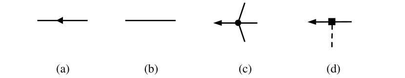
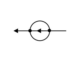
The bare propagators are easily read off from the Gaussian theory, corresponding to , indicated by the subscript . For the response propagator, shown in Fig. 4.1a, we find
| (41) | |||||
while the correlation propagator (Fig. 4.1b), also referred to as the correlator, is given by:
| (42) | |||||
The latter, of course, is just the dynamic structure factor for the Gaussian theory. A comparison of Eqns (39) and (42) allows us to identify the Gaussian, or mean-field, values of the critical exponents:
| (43) |
Clearly, these will acquire nontrivial corrections of .
The theory possesses only a single nonlinearity, easily identified from Eqn (37) as . In Fourier space, this gives rise to a four-point vertex, shown in Fig. 4.1c,
| (44) |
in Feynman integrals. Here, is the (transverse) momentum carried by the -leg. However, the expansion is not organized simply in powers of , as one can infer from an additional scaling symmetry of the theory: Due to the spatial anisotropy, parallel and transverse momenta (or lengths) can be rescaled independently, namely while remains unchanged. The functional, Eqn (37), is invariant under this transformation, provided we rescale and , so that is the invariant form of the nonlinearity. For convenience, we also absorb a geometric factor into the definition of the effective coupling constant:
| (45) |
In the following, we consider the critical theory, i.e., we set to zero in all propagators. However, does require renormalization which can be extracted from insertions of into graphs of the critical theory. As usual, the insertion corresponds to a two-point vertex, shown in Fig. 4.1d, carrying nonzero external momentum Pu . For later reference, we note that vertex functions with insertions can be resummed, to generate the vertex functions of the theory above FT .
Even though the detailed momentum dependence of propagators, vertex and insertion is of course different from Model B, the topology and combinatorics of the Feynman diagrams are identical. This helps to simplify some of the technicalities. For example, denoting bare one-particle irreducible vertex functions with () external - (-) legs and insertions as , it is straightforward to identify the primitively divergent ones as , , and . At the upper critical dimension, i.e., in , the last two of these both scale as . This momentum dependence is already carried by a factor of on one of the external legs, so that the remaining integrals are momentum-independent. In contrast, has the dimension of , so that the integral itself must contribute another factor of , in addition to the one carried by the external leg. Similar to Model B, each of the three vertex functions gives rise to one nontrivial renormalization, so that we anticipate two independent exponents provided an infrared stable fixed point can be found. All other vertex functions, including especially , are primitively convergent. It is now straightforward to evaluate these diagrams and extract the singularities. Relegating the details to the Appendix, we only quote the results:
| (46) | |||||
Here, as well as and are integrals defined in the Appendix.
Next, we renormalize our theory, by introducing a set of renormalized quantities (which are identified by the superscript ) and the associated -factors. These are related to the original (bare) set of quantities by:
| (47) | |||||
Note that is dimensionless, and can be used to define a renormalized effective coupling
| (48) |
which is, unlike , also dimensionless. Based on and , we consider a set of renormalized vertex functions:
| (49) | |||||
The renormalization conditions consist of demanding that all ’s be finite as . As a result, through Eqns (46) and (47), all renormalized quantities are implicitly dependent on – the (momentum) scale at which these conditions are imposed. Of the many routes to realize finiteness, the minimal subtraction scheme is the most facile. Only pure poles in need to be introduced in the -factors, to cancel those in the ’s. Thus, we can easily read off the results for the ’s.
First, we find to all orders in that
| (50) |
i.e., the couplings and require no renormalization while the -factors for the fields are inverse to one another. The remaining -factors must be determined order by order in perturbation theory. To two loops, we obtain
| (51) | |||||
where the expressions and are defined in the Appendix.
Once the (finite) ’s are known, we can find their scaling behavior in the infrared limit by studying their “flow” as . Since the bare ’s are independent of , flow equations FT for the ’s arise from applying , at fixed bare quantities, to Eqn (49):
| (52) |
where and the dots represent similar terms for the other parameters. Defering the complete equation until below, we focus on , which controls the flow of the effective coupling . To describe critical behavior, we seek infrared stable fixed points of the flow, i.e., zeroes of which are attractive under . In our case,
| (53) |
where . For , the only stable fixed point is the Gaussian . It becomes unstable below the critical dimension, i.e., in , to be replaced by a second, nontrivial fixed point which emerges smoothly from the origin:
| (54) |
Near , flows as
| (55) |
if initially. Here,
| (56) |
is positive (within perturbation theory), so that (54) is indeed stable. This is also a critical exponent, controlling corrections-to-scaling.
Having established the existence of an infrared stable fixed point below the upper critical dimension, we now focus on the scaling properties of our theory which can be extracted from the RG equation. The latter expresses the -independence of the bare vertex functions, at fixed bare parameters, as a differential equation for the renormalized vertex function. To begin with, let us introduce several additional Wilson functions:
| (57) |
where the symbol represents any of the variables , , , , or . Given the definitions of the couplings and the -factors computed above, these functions satisfy the following identities, valid to all orders in perturbation theory:
| (58) |
Thus, there are only two independent Wilson functions, and , whose expansions are easily computed up to . For the following, only their values at the fixed point are important:
| (59) | |||||
Finally, we recall that the vertex functions of the critical theory, with insertions of , are easily resummed to give the vertex functions of the disordered phase, at finite . Suppressing the superscript on all parameters for the sake of clarity, we quote the full RG equation:
| (60) | |||||
This equation can be solved, using the method of characteristics. In the immediate vicinity of the fixed point, where the theory exhibits scaling, we can incorporate dimensional analysis and the anisotropic scale transformation into the solution, whence:
Here, the overall scaling exponent is
| (62) |
and the parameter is just a scaling factor, as in Eqn (39). In Eqn (4.2.3), we list only those parameters in the argument that take an active part in the scaling form.
Let us illustrate how Eqn (39) emerges from the solution of the RG equation. To obtain the scaling form of the structure factor, we recall the connection between the two-point correlations and the two-point vertex functions:
Inserting the appropriate scaling forms, and performing a Fourier transform from the time- into the frequency domain yields Eqn (39):
In analogy with the scaling form of Model B, we now define two static exponents
| (63) |
and
| (64) | |||||
which are the only two independent indices. We emphasize that both of these differ from their counterparts for the Ising model near . Thus, the two-temperature model falls into a different universality class, defined by the dipolar system as shown by a comparison with the exponents quoted in BZ . However, a two-loop calculation is necessary in order to exhibit the differences between Model B and the dipolar system. At the order of one loop, retains its mean-field value, and is determined by combinatorics alone. Moving beyond statics, we find that the dynamic exponent is related to the static ones by the conservation law:
While this scaling law is also obeyed by the Model B exponents, the explicit result for is characteristic for the two-temperature model, as well as the dipolar system in the presence of a conservation law for the magnetization. Finally, we quote the strong anisotropy exponent , which controls the anisotropic scaling of parallel and transverse momenta:
Scaling laws relate all other exponents to these two, e.g., the “specific heat” exponent as discussed above.
The most interesting remaining index is the order parameter exponent which can be extracted from the equation of state. Since there are no dangerous irrelevant operators here, a simple scaling analysis is sufficient. In order to describe the effect of a magnetic field, we add a term to the dynamic functional. The transverse gradient operator imposes the (relevant) effect of the conservation law. Clearly, this will generate a nonvanishing, spatially varying magnetization, , which breaks the Ising symmetry of our system. Introducing the vertex generating functional , the equation of state for the renormalized quantities follows from
Here, the conservation law, reflected in the derivative , selects the first nonzero Fourier component of the right hand side. Expanding in powers of , the right hand side is reduced to a sum of vertex functions which are computed in the disordered phase:
The scaling form of the equation of state now follows directly from the solution of the RG equation, Eqn (4.2.3):
Choosing such that , the equation of state is recast in standard form
with an appropriately defined scaling function . We can now read off the magnetic-field exponent
and the order parameter exponent
5 Summary and Outlook
We have presented a detailed study of a non-equilibrium Ising system, with Kawasaki exchange dynamics coupled anisotropically to two thermal baths. Even when one of the baths is set at infinite temperature, this system is known to display a second order phase transition similar to the equilibrium model, with generic scale invariance at all temperatures above criticality glms ; epl . Both field theoretic renormalization group techniques and Monte Carlo simulations on 2-dimensional square lattices have been used. Excellent agreement between the two approaches is found for . Since this system displays strongly anisotropic scaling properties, we exploit finite size scaling with rectangular samples to control the effects of a new scaling variable associated with the aspect ratio (Eqn 17). The results are entirely consistent with the predictions of the field theory. By contrast, data from square samples fail to collapse, showing that the aspect ratio indeed plays a significant role.
One of the more intriguing aspects of this system is the following. The fixed point controlling critical properties can be associated with a uniaxial magnet with dipolar interactions in equilibrium. More specifically, the leading singularities in the thermodynamic functions of our non-equilibrium lattice gas are, in the critical region, identical to those for the equilibrium magnetic system. Of course, our lattice gas is still a bona-fide non-equilibrium system. To find these aspects, we must study either sub-leading singularities, such as corrections to scaling, or quantities associated with dangerous irrelevant operators dangIRO . A good example of the latter is the energy flux through the system, which is easily measured in simulations but quite difficult to compute theoretically.
Looking beyond this study, we see opportunities for further pursuit. Apart from the obvious need for better statistics and larger system sizes, there are many new avenues. To end this paper, we list a few. (a) Very little is known about this system below the critical point. Only the fluctuations of the interface were scrutinized KETTinterface . Correlations within each bulk phase are expected to be long-ranged, but confirmations from simulations are still lacking. Similar to the case of a uniformly driven lattice gas, domain growth during phase segregation is expected to display strongly anisotropic time scales DDScoarsen . Unlike that case, there is no particle-hole asymmetry in our model. As a consequence, there may be no serious disagreement between the microscopic lattice gas model and the mesoscopic Cahn-Hilliard like approach. (b) For the driven lattice gas, imposing open OBC or skewed-periodic SPBC boundary conditions leads to surprisingly different behavior, especially at low temperatures. Viable field theories for these systems are yet to be formulated. (c) On the other hand, a complete renormalization group analysis exists for multi-temperature models, as shown above. Though most of the predictions are mean-field like, it would be interesting to carry out simulations to confirm or disprove them.
Of course, this model represents only a small example in the vast field of systems in non-equilibrium steady states. Other models subjected to two thermal baths abound other TT , not to mention complex physical systems ranging from heating a pot on a stove to the ecosystem of the earth. Hopefully, the richness displayed in this very simple two-temperature model will spur further interest in pursuing other models and, most importantly, enhance our insights into this vast class of physical systems in non-equilibrium steady states.
ACKNOWLEDGMENTS
We thank A.D. Bruce, H.K. Janssen, O.G. Mouritsen, and Z. Rácz for many illuminating discussions. The computational assistance of H. Larsen is gratefully acknowledged. This research is supported in part by grants from the US National Science Foundation under DMR-9727574, NATO under OUTR.CRG 961238, and the Danish Natural Science Research Council under Snr. 9901699. One of us (RKPZ) thanks H.W. Diehl for his hospitality at the University of Essen, where some of this work was performed.
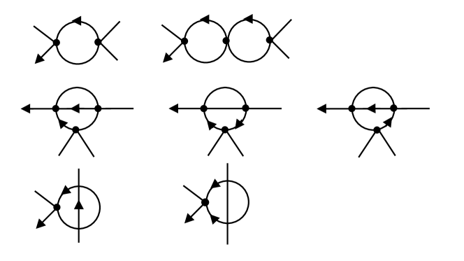
6 Appendix
In this appendix, we include some details of how to extract the singular parts of the three vertex functions of interest: and Figs. 6.2-4 show the corresponding Feynman graphs, up to and including two loops. Contributions that vanish in dimensional regularization or due to causality have already been omitted. We stress that we are only interested in the ultraviolet singular parts of the vertex functions, in the critical theory. To regularize the infrared behavior of our integrals, it is sufficient to keep transverse external momenta finite. Parallel external momenta and external frequencies may eventually be set to zero, since they contribute to finite terms only. The abbreviated notation will be used throughout.
The structure of at this order is:
| (65) | |||||
Any neglected terms involve at least three loops. This expression can be simplified considerably. First, it is straightforward to integrate over ’s, and the external may be set to zero. Next, we absorb the parallel diffusion coefficient into the parallel momenta, so that the effective coupling constant, Eqn (45), appears explicitly. Finally, we can recast the remaining momentum integrals in a more symmetric form, resulting in:
| (66) |
where the remaining integral (which still carries a nontrivial -dependence, as we will see below) is defined as
| (67) | |||||
In the second line, we have recognized that the momenta under the integral combine into three factors of the static Gaussian structure factor, Eqn (36). Thus, the resulting expression, up to a prefactor , is identical to the static two-point vertex function of the uniaxial dipolar ferromagnet, at two-loop order, with the correct momentum integrals and combinatoric factors! This structure reflects the restoration of the FDT, Eqn (38), and can be observed at each order in perturbation theory.
Similar reductions occur for the other two vertex functions. Let us demonstrate it for the one-loop graph of the (dynamic) four-point function, . Its calculation is further simplified by choosing transverse external momenta at a symmetry point, defined by
for . Up to one loop, the expression reads:
| (68) | |||||
Defining
| (69) | |||||
we write
| (70) |
Again, we recognize the zero-frequency part as the one-loop form of the static four-point function (up to a factor ), involving just static propagators. The explicit reductions at the two-loop level involve combinations of several dynamic diagrams into one static one. For brevity, we only quote the results, so that the leading singular parts of read:
| (71) |
where the last integral is given by
Finally, we turn to the last vertex function, namely which carries the insertion. As in Model B, the integrals contributing to are just those of : The insertion corresponds to two of the four external legs being “tied together”. In general, it carries both momentum () and frequency (), but the latter can be set to zero again. Thus,
| (73) |
It is now straightforward, if tedious, to evaluate these integrals and to extract the singularities. The one-loop diagrams present no difficulties. It is rather instructive, however, to consider one of the nontrivial two-loop diagrams as an example. We illustrate our procedure with the help of the integral contributing to :
| (74) |
First, we integrate over the parallel momenta. To do so, we recast the -function for the parallel momenta via its Fourier transform, leading to a product of three integrals of the form
| (75) |
The integral over is now easily performed, and the external may again be set to zero, resulting in
| (76) | |||||
The advantage is obvious: the extremely inconvenient -terms in the denominator have been reduced to quadratic () powers, in the process cancelling the -factors in the numerator. The remaining integral is of a much simpler form and requires only the familiar tools for evaluating standard -theory integrals FT . In a similar fashion, one can simplify the two-loop integrals for . Collecting our results for the integrals, we obtain, up to corrections:
Here, is Euler’s constant. The anticipated factor of is, finally, displayed explicitly in . It indicates that this integral is a correction to the zero-loop term in Eqn (66):
| (77) | |||||
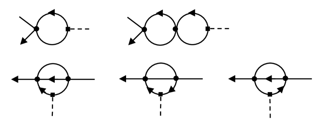
In the minimal subtraction scheme, only the pure -poles in the ’s and will be needed. Thus, we define
| (78) | |||||
where all corrections have been neglected. Note that, within this framework, is “more than the square of” .
References
- (1) S. Katz, J.L. Lebowitz and H. Spohn, Phys. Rev. B 28, 1655 (1983); J. Stat. Phys 34, 497 (1984).
- (2) B. Schmittmann and R.K.P. Zia, Phase Transitions and Critical Phenomena, Vol. 17, edited by C. Domb and J. L. Lebowitz (Academic, London, 1995).
- (3) See, e.g., S. Chandra, Superionic Solids. Principles and Applications (North Holland, Amsterdam 1981).
- (4) E. Ising, Z. Physik 31, 253 (1925).
- (5) P. L. Garrido, J. L. Lebowitz, C. Maes and H. Spohn, Phys. Rev. A42, 1954 (1990).
- (6) M. Q. Zhang, J. -S. Wang, J. L. Lebowitz and J.L. Vallés, J. Stat. Phys. 52, 1461 (1988); B. Schmittmann and R.K.P. Zia, J. Stat. Phys. 91, 525 (1998).
- (7) K. Hwang (1993), unpublished and K. Hwang, B. Schmittmann and R.K.P. Zia, Phys. Rev. E48, 800 (1993).
- (8) Z. Cheng, P. Garrido, J.L. Lebowitz, and J.L. Vallés, Europhys. Lett. 14, 507 (1991) and Garrido, et. al. in glms .
- (9) J. Marro, J.L. Vallés, and J.M. Gonzalez-Miranda, Phys. Rev. B35, 3372 (1987).
- (10) J.L. Vallés and J. Marro, J. Stat. Phys. 49, 89 (1987).
- (11) K.-t. Leung, Phys. Rev. Lett. 66, 453 (1991) and Int. J. Mod. Phys. C3, 367 (1992).
- (12) E. Praestgaard, H. Larsen, and R.K.P. Zia, Europhys. Lett. 25, 447 (1994).
- (13) J. S. Wang, J. Stat. Phys., 82, 1409 (1996).
- (14) K.-t. Leung and R.K.P. Zia, J. Stat. Phys., 83, 1219 (1996).
- (15) L. Onsager, Phys. Rev. 65, 117 (1944).
- (16) G. Grinstein, J. Appl. Phys. 69, 5441 (1991).
- (17) R.K.P. Zia, K. Hwang, K-t. Leung, and B. Schmittmann, in Computer Simulation Studies in Condensed Matter Physics V, eds. D.P. Landau, K.K. Mon, and H.-B. Schüttler, (Springer, Berlin, 1993).
- (18) B. Schmittmann and R.K.P. Zia, Phys. Rev. Lett. 66, 357 (1991).
- (19) B. Schmittmann, Europhys. Lett. 24, 109 (1993).
- (20) C.N. Yang and T.D. Lee, Phys. Rev. 87, 404 (1952); and T.D. Lee and C.N. Yang, Phys. Rev. 87, 410 (1952).
- (21) K. Kawasaki, Phys. Rev. 148, 375 (1966).
- (22) B.M. McCoy and T.T. Wu, The Two-dimensional Ising Model (Harvard Univ. Press, Cambridge, Mass., 1973).
- (23) K.G. Wilson and M.E. Fisher, Phys. Rev. Lett. 28, 240 (1972).
- (24) See, e.g., K.G. Wilson, Rev. Mod. Phys. 47C, 773 (1975); D.J. Amit, Field Theory, the Renormalization Group and Critical Phenomena, 2nd revised edition, (World Scientific, Singapore, 1984).
- (25) B.I. Halperin, P.C. Hohenberg, and S-k. Ma, Phys. Rev. B10, 139 (1974); J. Zinn-Justin, Quantum Field Theory and Critical Phenomena, (Oxford University Press, Oxford, 1996).
- (26) H.K. Janssen, Z. Phys. B23, 377 (1976); C. de Dominicis, J. Phys. (Paris) Colloq. 37, C247 (1976).
- (27) R. Kubo, Rep. Progr. Phys. 29, 255 (1966). See R. Graham, Z. Phys. 26 397 (1977) and B40, 149 (1980), for a much deeper discussion of this fundamental issue.
- (28) H. Risken, The Fokker-Planck Equation (Springer, Heidelberg 1989).
- (29) H.K. Janssen, in Dynamical Critical Phenomena and Related Topics, ed. C.P. Enz, Lecture Notes in Physics, Vol. 104 (Springer, Heidelberg, 1979).
- (30) P.C. Hohenberg and B.I. Halperin, Rev. Mod. Phys. 49, 435 (1977).
- (31) K. Binder, Z. Phys. B43, 119 (1981).
- (32) R.K.P. Zia, L.B. Shaw, and B. Schmittmann, Physica A279, 60 (2000).
- (33) R.K.P. Zia, L.B. Shaw, B. Schmittmann, and R.J. Astalos, Com. Phys. Comm. 127, 23 (2000).
- (34) G. Schüetz, in Phase Transitions and Critical Phenomena, Vol. 19, edited by C. Domb and J.L. Lebowitz (Academic, London 2000).
- (35) K. Hwang, B. Schmittmann and R.K.P. Zia, Phys. Rev. Lett. 67, 326 (1991) and Phys. Rev. E48, 800 (1993).
- (36) A.I. Larkin and D.E. Khmelnitskii, Zh. Eksp. Teor. Fiz. 56, 2087 [Sov. Phys.-JETP 29, 1123] (1969); A. Aharony and M.E. Fisher, Phys. Rev. B8, 3323 (1973); A. Aharony, Phys. Rev. B8, 3363 (1973); R.A. Cowley, Adv. Phys. 29, 1 (1980); A.D. Bruce, Adv. Phys. 29, 111 (1980).
- (37) E. Brézin and J. Zinn-Justin, Phys. Rev. B13, 251 (1976).
- (38) P.C. Martin, E.D. Siggia and H.H. Rose, Phys. Rev. A8, 423 (1973).
- (39) R.M. Hornreich, M. Luban, and S. Shtrikman, Phys. Rev. Lett. 35, 1678 (1975). See also Cowley and Bruce in dipolar .
- (40) See, e.g., D.J. Amit, Field Theory, the Renormalization Group and Critical Phenomena, 2nd revised edition, (World Scientific, Singapore, 1984) or Zinn-Justin in ZJ .
- (41) Instead of introducing an additional “field” renormalization, , for the insertion, we choose a “coupling constant” renormalization of the parameter . Both procedures are equivalent.
- (42) M.E. Fisher, in Renormalization Group in Critical Phenomena and Quantum Field Theory: Proceedings of a Conference, eds. J.D. Gunton and M.S. Green, (Temple University, Philadelphia, 1974).
- (43) R.K.P. Zia and K.-t. Leung, J. Phys. A24, L1399 (1992) and K.-t. Leung and R.K.P. Zia, Journal of Physics A26, L737 (1993).
- (44) C. Yeung, T. Rogers, A. Hernandez-Machado, and D. Jasnow, J. Stat. Phys. 66, 1071 (1992);S. Puri, K. Binder, and S. Dattagupta, Phys. Rev. B46, 98 (1992); S. Puri, N. Parekh, and S. Dattagupta, J. Stat. Phys. 75, 839 (1994); and F.J. Alexander, C.A. Laberge, J.L. Lebowitz, R.K.P. Zia, J. Stat. Phys. 82, 1133-1158(1996); A.D. Rutenberg and C. Yeung, Phys. Rev. E60, 2710 (1999).
- (45) D.H. Boal, B. Schmittmann, and R.K.P. Zia, Phys. Rev. A43, 5214 (1991).
- (46) J.L. Vallés, K-t. Leung, and R.K.P. Zia, J. Stat. Phys. 56, 43 (1989).
- (47) See, e.g., A.L. Toom, Probl. Peredachi. Info. 12, 78 and 220 (1976); C.H. Bennet and G. Grinstein, Phys. Rev. Lett. 55, 657 (1985); Z. Rácz, Phys. Rev. Lett. 55, 1707 (1985); M. Creutz, Ann. Phys. (N.Y.) 167, 62 (1986); M. Droz, Z. Rácz, and P. Tartaglia, Phys. Rev. A41, 6621 (1990); H.W.J. Blöte, J.R. Heringa, A. Hoogland, and R.K.P. Zia, J. Phys. A23, 3799 (1990); K.E. Bassler and R.K.P. Zia, Phys. Rev. E49, 5871 (1994); K.E. Bassler and Z. Racz, Phys. Rev. Lett. 73, 1320 (1994); A. Szolnoki, G. Szabó and O.G. Mouritsen, Phys. Rev. E55, 2255 (1997); and M.C. Sabra, H. Gilhoj and O.G. Mouritsen, Phys. Rev. E58, 3547 (1998).