Kondo ground state in a quantum dot with an even number of electrons in a magnetic field

Abstract

Kondo conduction has been observed in a quantum dot with an even number of electrons at the Triplet-Singlet degeneracy point produced by applying a small magnetic field $B$ orthogonal to the dot plane. At a much larger field $B\sim B_{*}$, orbital effects induce the reversed transition from the Singlet to the Triplet state. We study the newly proposed Kondo behavior at this point. Here the Zeeman spin splitting cannot be neglected, what changes the nature of the Kondo coupling. On grounds of exact diagonalization results in a dot with cylindrical symmetry, we show that, at odds with what happens at the other crossing point, close to $B_{*}$, orbital and spin degrees of freedom are “locked together”, so that the Kondo coupling involves a fictitious spin $1/2$ only, which is fully compensated by conduction electrons under suitable conditions. In this sense, spin at the dot is fractionalized. We derive the scaling equation of the system by means of a nonperturbative variational approach. The approach is extended to the $B\neq B_{*}$-case and the residual magnetization on the dot is discussed.

]

I Introduction

Low temperature transport properties of quantum dots (QD) are primarily determined by electron-electron interactions[1]. When a QD is weakly coupled to the contacts its charging energy is larger than the thermal energy. Therefore, in the absence of a source-drain voltage bias, $V_{sd}$, electrons can be added to the dot in a controlled way by changing an applied gate voltage, $V_{g}$ [2, 3]. Conductance peaks are separated by Coulomb Blockade (CB) regions, in which the electron number $N$ is fixed (Coulomb oscillations).

However, there is a well established experimental evidence for zero-bias anomaly in the conductance in a CB region when $N$ is odd [4, 5]. This occurs when the temperature is further decreased and the strength of the coupling to the contacts increased. Such a behavior is attributed to the formation of a Kondo-like hybridized state between the QD and the contacts [6, 7]. Kondo effect is not expected when $N$ is even, because of lack of spin degeneracy as the QD is in a singlet state. An exception is provided when a QD with $N$ even is in a triplet state because of Hund’s rule. In this case the QD shows a very peculiar spin-1 Kondo Effect [8, 9, 10, 11]. The Kondo anomaly is enhanced if the singlet state is close to be degenerate with the triplet. Such a regime can be achieved experimentally by applying a weak magnetic field orthogonal to the dot, $B_{\perp}$, because Hund’s rule breaks down quite soon. Correspondingly, the QD undergoes a triplet-singlet transition, which eventually suppresses the Kondo effect. In the following we shall refer to the transition above as “TS crossing”.

If the magnetic field is further increased, orbital effects induce the reverse transition from the singlet to the triplet state at some “critical field” $B_{\perp}=B_{*}$, in the general landscape of transitions to higher spin states [12, 13]. In this paper we focus on this transition, in the following referred to as “ST crossing”. The accidental degeneracy between states with different total spin can restore the Kondo effect. However, as we will show below, the presence of a substantial Zeeman splin splitting (Zss) makes the ST crossing very different from the TS crossing. Our analysis is an extension of the results of [14].

We consider a vertical QD with contacts located at the top and at the bottom of a pillar structure [2] (see Fig. 1a). Because the confining potential is chosen to be parabolic in the radial direction, single particle states on the dot are labeled by $(n,m,\sigma)$ where $n$ is an integer, $m$ is the orbital angular momentum and $\sigma$ the electron spin. We have chosen $N=2$ for sake of simplicity, but we believe that the pattern we describe is quite frequent. For example, it can be extended to the case when $N$=4.

Because of the Zss, the crossing occurring at the ST point involves the singlet and the $S^{z}=1$-component of the triplet state only. The analysis of the quantum numbers of the $N\pm 1$ states visited by virtual transitions (cotunneling processes ) shows that orbital and spin quantum numbers of the electrons involved are “locked together” (Fig. 2a). Tunneling from the contacts does not conserve $n$, but, since the geometry is cylindrical, it conserves $m$ and the spin. In particular, if the dot is in the triplet state, only $(m=0,\downarrow)$-electrons can enter it, while is it is in the singlet state, then only $(m=1,\uparrow)$-electrons enter. This envisages a one-channel spin 1/2-like Kondo coupling different from what occurs at the TS point.

The existence of a Kondo effect between states belonging to different representations of the total spin is very peculiar. Being the total dot spin of both the degenerate levels integer ($S=0,1$), spin compensation has to be incomplete. In this work we show that it is as if the total spin were decomposed into two fictitious spins $\frac{1}{2}$ which we refer to as $S_{r}$ and $S_{\text{\it eff}}$ [15]. We stress that these dynamical variables involve both orbital and spin degrees of freedom which are locked together. The magnetic field $B_{*}$ favors antiferromagnetic (AF) coupling between the delocalized electrons of the contacts and $S_{\text{\it eff}}$, which quenches it in the strong coupling limit. $S_{r}$ is the residual spin $\frac{1}{2}$ at the dot[16]. CB pins $N$ to an even value, but the correlated state that sets in will have half-odd spin, i.e., “fractionalization of the spin” at the QD site will take place [14]. $B_{*}$ only affects the magnetization related to $S_{r}$, but we will not discuss such a point in this paper. On the contrary, detuning $B$ from $B_{*}$ corresponds to an effective magnetic field $\delta B=B-B_{*}$, which affects Kondo screening.

On the other hand, at temperatures $T>T_{K}$ ( $T_{K}$ being the Kondo temperature), there is no Kondo correlation. Furthermore, being the dot in CB, the screening by the delocalized electrons is quite negligible. As long as $B<B_{*}$, the total spin is 0. For $B>B_{*}$, the total spin is 1. The spin density on the dot has a drastic change at $B_{*}$, while the charge density is only slightly affected. This is shown in Fig. 3a: for $B<B_{*}$ (singlet state) the spin density is zero, while it is half the charge density for $B>B_{*}$ (triplet state $S=1$ with $z-$ component $S_{z}=1$).

This shows that the total spin of the dot is the relevant dynamical variable in the correlation process that sets in when temperature is lowered, while the charge degree of freedom is frozen for $B\sim B_{*}$.

In Section IV we set up a variational technique similar in spirit to Yosida’s approach [18] for the construction of a trial wavefunction of the correlated Ground State (GS). We start from a Fermi sea (FS) of delocalized electrons of the contacts, times the impurity spin wavefunction and we project out states which do not form a singlet at the dot site. This is a modified version of the Gutzwiller projector and the results we obtain qualitatively reproduce the strongly-coupled regime of the Kondo model [7, 19, 20, 21]. Our formalism also allows us to discuss the $\delta B\neq 0$-case and to calculate “off-critical” quantities, like the magnetization, as a function of $\delta B$. In [14] we estimated the Kondo temperature $T_{K}$. It is slightly below the border of what is reachable nowadays within a transport measurement ($T_{K}\sim$ tens of mK). Instead, an Electron Paramagnetic Resonance (EPR) experiment could provide evidence for the fractionalization of the spin. At $T<T_{K}$, the system goes across the Kondo state when $B$ is moved across $B_{*}$. Partial compensation of the dot spin due to the local screening implied by the Abrikosov-Suhl resonance takes place at the QD site. The residual magnetization is the one of a spin-1/2 in all the range $B\sim B_{*}$. Therefore, in lowering the temperature, the response to the microwave field should also appear all the way from $B<B_{*}$ to $B>B_{*}$ and a temperature-dependent Knight shift of the frequency should occur. Moreover, this feature should be detectable, due to the enhanced susceptibility of the Kondo state.

Differently from the scenario described here, the TS crossing has a nonsymmetric behavior across the degeneracy point. Spin 1 Kondo effect should take place for $B$ prior to the degeneracy point, It is renforced at the TS transition, but no Kondo effect at all should occur when the GS is a singlet.

The paper is organized as follows:

• In Section II we show that $B_{*}$ makes only four levels involved in the Kondo coupling, in analogy to the single impurity spin $\frac{1}{2}$ Anderson model (AM). We discuss the strongly coupled regime of the system by briefly recalling the scaling theory of the AM and specify what we mean as spin fractionalization.

• In Section III we employ the Schrieffer-Wolff transformation to map our system onto an Effective Kondo model. We show that the corresponding interaction between $S_{\text{\it eff}}$ and the spin of the electrons from the Fermi sea is antiferromagnetic (AF), which generates the strongly coupled Kondo regime.

• In Section IV we construct a trial GS using a modified version of the Gutzwiller projection method. We calculate the energy, which depends on the exchange interaction: $j$. We show that $j$ scales according to Anderson’s poor man’s scaling [22].

• In Section V we extend our technique to the $\delta B\neq 0$-case. Because of the presence of $\delta B$, a second scaling parameter, $h$, arises. We compute the energy and the magnetization as a function of $h$ and discuss how this is related to the bare field $\delta B$.

• In Section VI we report our final remarks and conclusions.

II The model for the dot at the level crossing ($B=B_{*}$).

Using exact diagonalization[13], two of us studied few interacting electrons in two dimensions, confined by a parabolic potential in the presence of a magnetic field $B$ orthogonal to the dot disk ($z-$direction). We chose the energy separation between the levels of the confining potential $\hbar\omega_{d}$ to be of the same size as the effective strength of the Coulomb repulsion $U$ ($\sim 4meV$), which makes the correlations among the electrons relevant. The magnetic field favors the increase of the total angular momentum in the $z-$ direction, $M$, as well as of the total spin of the dot, $S$, in order to minimize the Coulomb repulsion. The $B$-dependence of the spectrum of the QD energy levels can be monitored via a linear transport measurement, by attaching electrodes to it in a pillar structure (Fig. 1) [4, 5, 9]. At special values $B=B_{*}$, one can identify several level crossings between states with different $M$ and $S$.

In this paper we shall focus onto a QD with $N=2$ electrons, but the features we discuss here are appropriate for dots with any even $N$. The parameters of the device can be chosen such that $B_{*}$ is rather large, which lifts the spin degeneracy, because of Zeeman spin splitting [23]. We define $B_{*}$ as the field at which the GS of the isolated dot switches from singlet ($~{}^{2}S^{0}_{0}$; $S=0,M=0$) to the triplet state lowest in energy (the state $S_{z}=1$ of the three states $~{}^{2}T^{1}_{0,\pm 1}$: $S=1,M=1$ and $S^{z}=0,\pm 1$).

Only two $N=2$ states are primarily involved at the level crossing, namely, the $S=0$ singlet and the $S=1,M=1,S^{z}=1$ component of the triplet (see Fig. 2a). At the same $B$, the low lying $N=1$ and $N=3$-GS’s are spin doublets. We shall denote them as $~{}^{1}D_{\frac{1}{2}}^{0}$ and $~{}^{3}D_{\frac{1}{2}}^{1}$, respectively. Lifting the spin degeneracy makes the $S^{z}=\frac{1}{2}$ components lower in energy in both cases. If $V_{g}$ is tuned in the CB region between $N=2$ and $N=3$ (Fig. 1b), only the four states listed above are primarily relevant for the conduction.

We now construct a model by taking the 1-particle state , $~{}^{1}D_{\frac{1}{2}}^{0}$, as the “vacuum” of the truncated Hilbert space $\Xi$ (which we denote by $|0\rangle$). Let us take $|0\rangle$ to be the initial state of the QD. The dot can exchange one electron at a time with the contacts. A $(q,m,\uparrow)$-electron entering the QD generates a transition between $|0\rangle$ and $~{}^{2}T^{1}_{1}$. Alternatively, the lowest energy state available for a $(q,m,\downarrow)$-electron entering the QD is the singlet $~{}^{2}S_{0}^{0}$ (here $q$ is the modulus of the momentum of the particles and $m$ is the azimuthal quantum number, which is conserved by the interaction with the dot). It is useful to define the operators $d_{1,2}^{\dagger}$ which create the two $N=2$ many body states $|\alpha\rangle$ ($\alpha=1,2)$, belonging to $\Xi$, by acting on $|0\rangle$:

$$|1\rangle\equiv|~{}^{2}S^{0}_{0}\rangle=d_{1}^{\dagger}|0\rangle;\>\>\>|2\rangle\equiv|~{}^{2}T^{1}_{1}\rangle=d_{2}^{\dagger}|0\rangle$$ (1)

The operator $d_{1}^{\dagger}/d_{2}^{\dagger}$ adds a $(m=0,\downarrow)/(m=1,\uparrow)$ electron to the dot. Finally, the state $|3\rangle$ is defined as: $|3\rangle\equiv|~{}^{3}D_{\frac{1}{2}}^{1}\rangle=d_{2}^{\dagger}d_{1}^{\dagger}|0\rangle$. The operators $d_{1,2}$ defined above cannot be associated to any single particle function on the dot. Nevertheless, as far as low-energy excitations only are involved, it is a good approximation to take them to be anticommuting. To show this we refer to Fig. 4, where we report the calculated quasiparticle spectral weight, when an extra electron is added to the dot in one of the two possible GS’s at $B=B_{*}$ and $N=2$. In Fig. 4a we show the weight for addition of an extra particle to the state $|~{}^{2}T^{1}_{1}\rangle$ to give a state with total angular momentum $M=1$. This is close to 1 for a $\downarrow$-spin but is practically zero at low energies for an $\uparrow$ spin because states with $S=3/2$ are higher in energies. According to the definitions of eq.(1), this implies that, while the state $d_{1}^{\dagger}d_{2}^{\dagger}|0\rangle$ can be normalized, one has $(d_{2}^{\dagger})^{2}|0\rangle\approx 0$. Analogously, Fig. 4b shows that there is an energy shift of the spectral weight peak when a $\uparrow$ or a $\downarrow$ spin particle is added to the state $|~{}^{2}S^{0}_{0}\rangle$. This shift corresponds to the Zeeman spin splitting between the states ${}^{3}D^{1}_{\frac{1}{2}}$ and ${}^{3}D^{1}_{-\frac{1}{2}}$. We ignore the latter that is placed at higher energy. In Section III we argue that inclusion of this state does not qualitatively change our results. Then, within this approximation that includes the lowest energy state only, we take $(d_{1}^{\dagger})^{2}|0\rangle\approx 0$. So, we are alleged to assume $(d_{1,2}^{\dagger})^{2}=0$. Hence, the $d$-operators behave as they were single-particle fermion operators, although, in fact, they create many-particle states.

We write the Hamiltonian for the QD as:

$$H_{D}=\epsilon_{d}(n_{1}+n_{2})+Un_{1}n_{2}$$ (2)

where $n_{\alpha}=d_{\alpha}^{\dagger}d_{\alpha}$, $\epsilon_{d}$ is the energy of the degenerate $N=2$ levels and $U$ is the charging energy for adding a third electron.

We assume the electrons in the leads to be noninteracting. Let $b_{jq\sigma}$ be the annihilation operators for one electron in the left ($j=L$) and the right ($j=R$) contact, respectively, and let $\epsilon_{q}$ be the corresponding energy (independent of $j$ and $\sigma$ for simplicity). The Hamiltonian for the leads is:

$$H_{l}=\sum_{q\sigma}\sum_{j=L,R}\epsilon_{q}b_{jq\sigma}^{\dagger}b_{jq\sigma}$$ (3)

We denote by ${\cal{H}}_{0}=H_{D}+H_{l}$ the sum of the two Hamiltonian terms given by eqs.(2,3). They do not change the particle number $N$ on the dot. Instead, $N$ is changed by tunneling between the leads and the dot, according to the above mentioned selection rules. Let $\Gamma_{R}$ and $\Gamma_{L}$ be the amplitudes for single-electron tunneling between the dot and the $R$ or $L$ contact, respectively. Removal of one electron from the contacts is described by the following linear combination of the $b_{jq\sigma}$’s:

$$\phi_{q\sigma}\equiv\frac{1}{\sqrt{|\Gamma_{L}|^{2}+|\Gamma_{R}|^{2}}}(\Gamma_{L}b_{Lq\sigma}+\Gamma_{R}b_{Rq\sigma})$$ (4)

For a point-like QD, there will be no tunneling term involving the combination of $b_{jk\sigma}$ operators linearly independent of $\phi_{q\sigma}$. The terms to be added are $(\alpha=1,2)$:

$$V_{\alpha 0}=\sum_{q}v_{\alpha 0}^{*}(q)d_{\alpha}^{\dagger}\phi_{q\sigma_{\alpha}}$$ (5)

for $N=1\to N=2$ and:

$$V_{3\alpha}=\sum_{q}v_{3\alpha}(q)d_{\bar{\alpha}}^{\dagger}\phi_{q\sigma_{\bar{\alpha}}},$$ (6)

for $N=2\to N=3(\bar{\alpha}\neq\alpha)$ . Because spin is conserved in the tunneling is $\sigma_{1}=\downarrow$, and $\sigma_{2}=\uparrow$ and $\bar{\alpha}\neq\alpha$. Hermitian conjugate operators of $V_{\alpha 0}$ and $V_{3\alpha}$ decrease the electron number on the dot.

This model Hamiltonian has the form of the nondegenerate Anderson Model (AM). In [14] we have considered a special choice of the $V_{g}$ fine tuning (see Fig. 1b), which corresponds to the symmetric case: the singly occupied localized impurity level has energy $\epsilon_{d}=-U/2$, while the doubly occupied one has energy $\epsilon_{d}+U=U/2$. Also, $\Gamma_{j}\>\>(j=L,R)$ have been taken independent on $j$.

Integration over the contact fields $\phi_{q\sigma}$ in the partition function leads to the constrained dynamics of the dot between the two degenerate states $|\alpha\rangle$, labeled by $\alpha=1,2$ and coupled to an external fluctuating field $X(\tau)$ [24]. As shown in [14], the main contributions to the partition function are the quantum fluctuations of an effective fictitious spin $\frac{1}{2}$ $S_{\text{\it eff}}$, due to the coupling among the dot and the leads. This spin flips from 1 to 2 because of cotunneling processes in which an $(m=1,\uparrow)$ electron is added/removed in the dot while an $(m=0,\downarrow)$ electron is removed/added (see Fig. 2a ) Its quantum dynamics produces a correlated state between dot and leads in which the charge excitations, being higher in energy, are fully decoupled and suppressed. Four states are available prior to correlation, corresponding to $S=0,1$, two of which are degenerate. They factorize according to the decomposition law:

$$\vec{S}=\vec{S_{r}}+\vec{S}_{\text{\it{eff}}}.$$ (7)

where $S_{r}$ is a residual spin $1/2$ whose wavefunction factorizes close to $B_{*}$. Correlation with the contacts is governed by a single channel spin $\frac{1}{2}$ AF Kondo Hamiltonian for $S_{\text{\it eff}}$, which is derived in Section III and discussed in detail in Appendix A. In the corresponding GS, $S_{\text{\it eff}}$ is fully compensated as in the usual Kondo Effect at zero magnetic field.

In Sect. III and IV we show that, provided that the coupling to the leads is symmetrical for $\alpha$=1,2, the GS is doubly degenerate at $B=B_{*}$ (the limiting states are derived from the $|g^{\lambda}\rangle$ $(\lambda=\pm)$ of eq.(18), having energy $\epsilon(\xi,j)$ given by eq.(25)). The degeneracy disappears when is $\delta B=B-B_{*}\neq 0$ (see Fig.2b). Such a spin fractionalization closely resembles quantum number fractionalization in strongly-correlated 1-dimensional electron systems [25].

III Effective AF Kondo interaction.

In the previous Section we have introduced the four states $|i\rangle$, $i=0,1,2,3$ , which are primarily relevant to the low-temperature dynamics of the QD (see eq.(1)). Tuning $V_{g}$ as described in Section II (see Fig. 1b) allows only the $N=2$ states, $|1\rangle$ and $|2\rangle$, to be the initial and final states of any process. Let $\Xi$ be the subspace they span. The $N\neq 2$-states, $|0\rangle$ and $|3\rangle$, play a role only as virtual states allowing for higher-order tunneling processes. Then, it is desirable to describe the dynamics of the dot in terms of an effective Hamiltonian acting on $\Xi$ only. This is accomplished in this Section, by employing the Schrieffer-Wolff (SW) transformation at second order in the tunneling amplitudes.

According to eqs.(2,3 ) the elements of ${\cal H}_{0}$ are diagonal in the Fock space and are given by:

$$H_{00}=H_{l};\;H_{11}=H_{22}=H_{l}+\epsilon_{d};\;H_{33}=H_{l}+U+2\epsilon_{d}$$ (8)

$H_{03}=H_{12}=0$, while the tunneling part of the Hamiltonian of eq.s (5,6) provides the remaining off-diagonal terms $H_{ij}$ $(i,j=0,1,2,3)$.

The effective Schrödinger equation projected onto $\Xi$ is:

$$P[({\cal H}_{0}-E)-V^{\dagger}(1-P)({\cal H}_{0}-E)^{-1}V]P|\Psi\rangle=0$$ (9)

where $P$ is the corresponding projection operator.

For the sake of simplicity we shall take $v_{3\alpha}(q)$ and $v_{\alpha 0}(q)$ to be independent of $\alpha$. Then, to second order in $v$, eq.(9 ) becomes (see Appendix A for details):

$$H^{\rm\text{\it eff}}=H_{l}+\sum_{qq^{\prime}}Q_{qq^{\prime}}\sum_{\sigma}\phi_{q\sigma}^{\dagger}\phi_{q^{{}^{\prime}}\sigma}+$$ (10)

$$\sum_{qq^{\prime}}J_{qq^{\prime}}\sum_{a}\vec{S}_{\text{\it eff}}^{a}\phi_{q\lambda}^{\dagger}\sigma^{a}_{\lambda\lambda^{{}^{\prime}}}\phi_{q^{{}^{\prime}}\lambda^{{}^{\prime}}}$$ (11)

where $\sigma_{\lambda\lambda^{\prime}}^{a}$ are the spin $\frac{1}{2}$ matrices $(a=x,y,z)$ and $\vec{S}_{\text{\it eff}}$ is a spin-$\frac{1}{2}$ representation of the rotation within $\Xi$, which is well defined, provided the constraint $n_{1}+n_{2}=1$ is satisfied. Indeed, in this case, $(\vec{S}_{\text{\it eff}})^{2}$ = $\frac{3}{4}(n_{1}+n_{2}-2n_{1}n_{2})=\frac{3}{4}$. More explicitly: $S_{\text{\it eff}}^{z}=\frac{1}{2}(d^{\dagger}_{2}d_{2}-d^{\dagger}_{1}d_{1})$ and the ladder operator is $S_{\text{\it eff}}^{-}=d^{\dagger}_{1}d_{2}$.

The interaction matrix elements are

$$Q_{qq^{\prime}}=-\frac{1}{2}\left[\frac{v^{*}_{3}(q)v_{3}(q^{{}^{\prime}})}{\epsilon_{d}+U-\epsilon_{q}}+\frac{v_{0}(q)v^{*}_{0}(q^{{}^{\prime}})}{\epsilon_{d}-\epsilon_{q^{{}^{\prime}}}}\right]\>,$$ (12)

$$J_{qq^{\prime}}=2\left[\frac{v^{*}_{3}(q)v_{3}(q^{{}^{\prime}})}{\epsilon_{d}+U-\epsilon_{q}}-\frac{v_{0}(q)v^{*}_{0}(q^{{}^{\prime}})}{\epsilon_{d}-\epsilon_{q^{{}^{\prime}}}}\right]\>,$$ (13)

corresponding to the potential scattering term and the Kondo coupling term, respectively.

The potential scattering term $Q_{qq^{\prime}}$ provides a one-body interaction in the “charge” channel. It is irrelevant for the physics of the Kondo effect, which is related to interactions in the “spin” channel [20], and we shall disregard it in the following.

By taking $q$ at the Fermi surface, the Kondo term in eq.(11) becomes:

$$H_{K}=H^{\rm eff}-H_{l}\sim J\vec{S}_{\rm\text{\it eff}}\cdot\sum_{qq^{{}^{\prime}}}\phi_{q\lambda}^{\dagger}\vec{\sigma}_{\lambda\lambda^{{}^{\prime}}}\phi_{q^{{}^{\prime}}\lambda^{{}^{\prime}}}.$$ (14)

Tuning $V_{g}$ such that the chemical potential of the leads is the zero of the single-particle energies, the Kondo coupling strength in eq.(13) takes the usual form:

$$J=|V|^{2}\left[\frac{1}{\epsilon_{d}+U}-\frac{1}{\epsilon_{d}}\right]$$ (15)

$\epsilon_{d}\approx-U/2$ implies $J>0$, i.e., the interaction between the spin density of the Fermi sea at the location of the dot and the effective spin $S_{\text{\it eff}}$, described by eq.(14), is antiferromagnetic. Thus, the low-energy physics of the system will be controlled by the strongly coupled AF- $S=\frac{1}{2}$-Kondo fixed point, where a spin singlet takes place at the impurity site. Because of the way $S$ is related to $S_{\rm eff}$ (eq.(7 )), total compensation of $S_{\rm eff}$ leads to a spin $S=\frac{1}{2}$ at the QD.

In the next Section we will make use of such an equivalence to construct a formalism for the strongly coupled fixed point of our system.

IV Gutzwiller projection.

In Section II we have shown that cotunneling at the ST point strongly involves just two among the four available states of the isolated dot, which can be described in terms of $S_{\text{\it eff}}$, including both orbital and spin degrees of freedom locked together. Instead, the other relevant degrees of freedom of the dot can be lumped into another pseudospin variable $\vec{S}_{r}$ ($S_{r}=\frac{1}{2}$) which decouples below $T_{K}$, because the dot is tuned at CB (eq.(7)). According to Section III the dynamics of correlations involves the true spin density of the delocalized electrons at the dot site $\vec{\sigma}(0)$. Therefore, the study of the magnetization in the correlated state requires the knowledge of $\vec{\sigma}(0)$.

In Section III we discuss the assumptions under which the isotropic single channel spin $\frac{1}{2}$ AF Kondo model of eq.(14) describes the physics at the fixed point. The correlated state is a Noziéres local Fermi Liquid (FL) [26], with a spin singlet at the origin. In our case there is a substantial magnetic field $B\sim B_{*}$ and a small detuning $\delta B\neq 0$ is likely to occur.

In this Section, we construct an approximated GS of the strongly coupled system, described by $H^{\text{\it eff}}$ (eq.(14)). In order to describe the scaling of $S_{\text{\it eff}}$ toward total compensation, we use a variational method based on the Gutzwiller projection (GP) technique. This qualitatively reproduces the main features of the correlated singlet state. Detuning $B$ off $B_{*}$ allows for probing the QD magnetization and for studying the magnetic response in the correlated state. So, in Section V we extend our approach to the $B\neq B_{*}$-case.

As $J$ increases, states other than a singlet at the impurity become higher in energy and can be “projected out” from the physical Hilbert space. This is quite similar to what happens in the 1-d Hubbard model at large $U$, where higher-energy states are “projected out” by the interaction and the GP method works successfully [27]. Our approach is similar in spirit to Yosida’s variational technique [18]. However, here we are mostly interested in the “macroscopic” variable $\vec{\sigma}(0)$. Hence, it is the only lead operator involved in the construction of the variational state. This makes our technique much simpler than the one in [18], because our approach requires just one variational parameter for the trial state.

Here we list the basic assumptions concerning the model Hamiltonian and the trial variational state. We introduce our approach for the simple spin-$\frac{1}{2}$ Kondo Hamiltonian (which corresponds to $B=B_{*}$). In Section V we generalize it to the $\delta B\neq 0$-case. To simplify the notation, we drop the suffix ${}_{\text{\it{{eff}}}}$ from $S_{\text{\it eff}}$ all throughout this Section and the next one.

  a.

The Hamiltonian is (see eq.(14)):

$$H=H_{l}+H_{K}=H_{l}+Ja\vec{\sigma}(0)\cdot\vec{S}$$ (16)

The impurity is located at $x=0$. The scattering is $s$-wave, so that the model is effectively 1-d and can be defined on a lattice with spacing $a$ and periodic boundary conditions at $L=N_{l}a$. ($N_{l}$ is the number of lattice sites ) [28]. $H_{K}$ provides an effective interaction among the delocalized electrons. At each stage of the scaling process, we take the Slater determinant $|FS\rangle=\prod_{\sigma}\prod_{q<0}c_{q\sigma}^{\dagger}|0\rangle$ as a reference state (FS: Fermi sea). The $c_{q\sigma}$ operators annihilate the quasiparticles and $|0\rangle$ is the quasiparticle vacuum. The spectrum is linearized around the Fermi point $q_{F}$. $D$ is the bandwidth. Therefore, the lead Hamiltonian is $H_{l}=\sum_{q\sigma}\epsilon_{q\sigma}c_{q\sigma}^{\dagger}c_{q\sigma}$, where $\epsilon_{q\sigma}=v_{F}q$. Here $v_{F}$ is the Fermi velocity and $q$ is the momentum measured with respect to the Fermi momentum. The bandwidth is $2D=2\pi v_{F}/a$. The density of states at the Fermi level is $\nu(0)=N_{l}/D$ and is assumed to be constant during the scaling.

  b.

One can represent the real space field operator in terms of the $c$-operators:

$$\psi_{\sigma}(x)=\frac{1}{\sqrt{L}}\sum_{q}e^{iqx}c_{q\sigma}.$$ (17)

It satisfies the anticommutation relations $\{\psi_{\sigma}^{\dagger}(x),\psi_{\sigma^{{}^{\prime}}}(x^{{}^{\prime}})\}=\frac{1}{a}\delta_{\sigma,\sigma^{{}^{\prime}}}\delta_{x,x^{{}^{\prime}}}$.

The quantity $an_{\sigma}(0)=a\psi_{\sigma}^{\dagger}(0)\psi_{\sigma}(0)$ plays the role of the occupation number at the impurity site. This is consistent with the operator identity $(an_{\sigma}(0))^{2}=an_{\sigma}(0)$. The corresponding spin amplitude due to the delocalized electrons at $x=0$ is $a\vec{\sigma}(0)=\frac{1}{2}a\psi_{\alpha}^{\dagger}(0)\vec{\sigma}_{\alpha\alpha^{{}^{\prime}}}\psi_{\alpha^{{}^{\prime}}}(0)$. The average value of $(a\vec{\sigma}(0))^{2}$ on $|FS\rangle$ is: $\langle FS|(a\vec{\sigma}(0))^{2}|FS\rangle$=3/8. This is a consequence of averaging over configurations with zero or double occupancy at $x=0$ (total spin 0) and configurations with single occupancy at the same point (total spin 1/2).

  c.

The correlation between the impurity and the FL is accounted for by projecting out of the uncorrelated state the components with a triplet or a doublet of the total spin at the impurity site, $\vec{S}+a\vec{\sigma(0)}$.

Denoting the projector as $P_{g}$, the variational trial state is defined as:

$$|g^{\lambda}\rangle=P_{g}|FS,\lambda\rangle\equiv P_{g}\left(|FS\rangle\otimes|\lambda\rangle\right)\>.$$ (18)

Here $|\lambda\rangle$ is an eigenstate of $S^{z}$ with eigenvalue $\frac{1}{2}\lambda=\pm\frac{1}{2}$ and $g$ is the variational parameter. The explicit form of the Gutzwiller projection operator $P_{g}$ will be given below. So far, it is enough to say that all the components of the state other than a localized singlet at $x=0$ are projected out, as $g$ changes from zero to the limiting value, $g=4/3$.

  d.

At $B=B_{*}$, we assume the usual one parameter scaling process when $D\to D-\delta D$. $g$ approaches 4/3, and, in order to to guarantee that at each step the total energy is at a minimum, the parameter $\nu(0)J$ is correspondingly renormalized. If $\delta B=B-B_{*}\neq 0$, a second parameter appears in the model, related to $\delta B$. We shall refer to such a parameter as $h$ and will introduce it in the next Section. It is generated by the shift in the quasiparticle energies, according to their spin and will determine the “off-critical” magnetization (see point e).

  e.

According to eq.(7), the effective magnetization of the dot is given by the average of the total spin at $x=0$ on the trial state $|g^{\lambda}\rangle$ (shortly denoted by $\langle...\rangle_{g,\delta B}$):

$$\lim_{g\to 4/3}\left\{M_{d}(g,\delta B)-M_{d}(g,\delta B=0)\right\}$$ (19)

$$\approx\lim_{g\to 4/3}g^{*}\mu_{B}\left[\langle S_{\text{\it eff}}^{z}\rangle_{g,\delta B}+\langle a\sigma^{z}(0)\rangle_{g,\delta B}\right]$$ (20)

$$\equiv M_{imp}+m(h)\>\>.$$ (21)

Here we have temporarily restored the suffix _eff, for clarity. The dot magnetization $M_{d}$ includes the local moment on the impurity site $M_{imp}$, and the induced magnetic moment of the delocalized electrons from the contacts, $m(h)$.

At $\delta B=0$ both $M_{imp}$ and $m(h)$ vanish, due to the compensation of the effective spin $S_{\text{\it eff}}$ of the standard spin $\frac{1}{2}$ AF Kondo problem. $M_{d}(g,\delta B=0)$ is the residual magnetization at $B=B_{*}$ associated to the expectation value of $S_{r}$ of eq.(7) and is not discussed in this paper. However, the spin susceptibility of $S_{r}$ is expected to be much smaller than the Kondo susceptibility of $S_{\text{\it eff}}$.

One remark concerns the fact that the giromagnetic factor in eq.(21) might not be the bare one, appearing in the electron Zeeman spin splitting.

In Section V we work out the form of $M_{imp}$ and $m(h)$ in the strongly coupled scaling regime.

Let us now construct $P_{g}$.

According to Noziere’s FL picture of the correlated Kondo state [26], the main effect of the interaction between the FS and the impurity taken at the AF fixed point is to fully project out the components of the trial state other than a singlet of the total spin at the impurity site. Let us consider the operator

$$a\vec{\sigma}(0)\cdot\vec{S}=\frac{1}{2}[(a\vec{\sigma}(0)+\vec{S})^{2}-\frac{3}{4}-(a\vec{\sigma}(0))^{2}]$$ (22)

It will give zero when acting on a state that has a doublet on the impurity site, (i.e. $\langle(a\sigma(0))^{2}\rangle=0$), $-3/4$ when acting on a singlet, $1/4$ when acting on a triplet. Among the three possibilities listed above, the state corresponding to the triplet is the one highest in energy. We fully exclude it from the trial state from the outset and gradually project out the doublet by varying the parameter $g$ from 0 to 4/3. Accordingly, we define $P_{g}$ as:

$$P_{g}=\left(1-\frac{3}{4}g-ga\vec{\sigma}(0)\cdot\vec{S}\right)(1-4a\vec{\sigma}(0)\cdot\vec{S})=$$ (23)

$$\left(1-\frac{3}{4}g+g(a\vec{\sigma}(0))^{2}\right)-4a\vec{\sigma}(0)\cdot\vec{S}$$ (24)

This operator projects out the components other than the localized singlet. When $g$=4/3 the projection is complete.

In this section we report the result for the zero magnetic field case. The key points of the calculations are summarized in Appendix B.

The expectation value of the Hamiltonian in eq.(16) differs from the energy of the reference Fermi sea $|FS\rangle$, $E_{0}=-2\pi v_{F}N_{l}/a$, just by a term of order $O(1)$ in the particle number $N_{l}$. In units of $D$, this correction is:

$$\epsilon(\xi,j)=\frac{1}{D}\left(\frac{\langle g^{\lambda}|H|g^{\lambda}\rangle}{N[\xi]}-E_{0}\right)=2\frac{1+\xi^{2}-\xi-j}{1+\xi^{2}}$$ (25)

where $N[\xi]$ is norm of the trial state (see eq.(B2)) and we have introduced the dimensionless variables $j=3\nu(0)J/(8N_{l})$ and $\xi=\frac{3}{8}(\frac{4}{3}-g)$ for convenience.

It is worth stressing that $\epsilon(\xi,j)$ does not depend on the polarization of the impurity, $\lambda$. Such a degeneracy disappears when $\delta B\neq 0$[29].

For each $j\propto J/D$, eq.(25 ) takes a minimum as a function of $\xi$ (i.e. $g$). The minimum $\overline{\xi}(j)$ w.r.t. $j$ is given by:

$$\overline{\xi}(j)=-j+\sqrt{j^{2}+1}$$ (26)

Both the triplet and the doublet are fully projected out of the trial GS when $g\to 4/3$, i.e. when $\overline{\xi}$ flows to zero. Eq.(26) shows that this limit corresponds to $j\rightarrow\infty$.

The derivative of eq.(26) w.r.t. $\overline{\xi}$, reproduces the poor man’s scaling law for $j$ [22] provided $g$ is small (that is, $\xi$ is close to 1/2) :

$$\frac{dj}{d(ln\xi)}\approx-j^{2}.$$ (27)

Eq.(27) has been worked out in [22] within perturbation theory, provided $g$ is small, that is, $\xi$ is close to $\frac{1}{2}$. In our simplified approach , eq.(26) (not eq.(27) !) holds all the way down to the fixed point.

V The magnetic moment

In this Section we qualitatively discuss what happens to the energy and to the magnetic moment of the dot when a magnetic field is present and $B$ is possibly detuned off $B_{*}$.

Here we do not consider the in detail the magnetic moment associated to $S_{r}$. Instead, we focus on the one in the third line of eq.(21). We generalize the construction of Sect IV to the $\delta B\neq 0$-case by shifting the energies of the quasiparticles of the FS according to their spin. Two corrections to the magnetic moment arise due to this shift: $a)$ $\langle S_{\text{\it eff}}\rangle_{g,B}$ may not scale down to zero, $b)$ an induced moment of the delocalized electrons $m(h)$ may arise. We first discuss the latter contribution. In the absence of correlations, because $B_{*}$ is the degeneracy point, the energy difference of electrons involved in cotunneling at the Fermi level is the same for both spins. Therefore, provided also the density of states of the conduction electrons is the same at the Fermi energy for both spins, $B_{*}$ will only be responsible for changes in the tunneling Hamiltonian due to orbital effects [30], which do not influence the flow to strong coupling in a relevant way.

This is not the case if $\delta B\neq 0$. Qualitatively, there will be changes in the number of the conduction electrons involved, according to their spin $\sigma=\pm\frac{1}{2}$ as follows:

$$\frac{N_{\sigma}-N_{l}/2}{N_{l}/2}=\sigma\delta B\frac{\nu(0)}{N_{l}}=\sigma\frac{\delta B}{D}$$ (28)

The interaction modifies eq.(28) by scaling, so, we generalize it by defining a dimensionless quantity $h$ in terms of the expectation value of the quasiparticle spin at the origin evaluated on the reference state $|FS\rangle$:

$$\langle FS,\lambda|a\sigma^{z}(0)|FS,\lambda\rangle_{\delta B\neq 0}=$$ (29)

$$\langle FS,\lambda|\frac{1}{2}\left(an_{\uparrow}(0)-an_{\downarrow}(0)\right)|FS,\lambda\rangle\equiv\frac{1}{2}h_{\lambda}\>,$$ (30)

($h_{\lambda}=\lambda\cdot h$, where $\lambda=\pm$ is the polarization of the impurity ). Eq.(30) states that the magnetic field produces a spin density at the impurity site proportional to $h$. When $\delta B=0$, rotational symmetry of the FS implies $h=0$ unless a local paramagnetism takes place, so that $h$ is a homogeneous function of $\delta B$.

Eq.(30) is enough to generalize eq.(25) to the $\delta B\neq 0$-case. Using the results of of Appendix B, we get:

$$\epsilon_{\lambda}(\xi,h,j)=$$ (31)

$$\frac{[2(1-\xi+\xi^{2})+h_{\lambda}(1-2\xi)](1-h_{\lambda})-2j(1+h_{\lambda})}{[(1+h_{\lambda})+\xi^{2}(1-h_{\lambda})]}$$ (32)

As in the previous Section, the minimum of eq.(32) $w.r.t.\>\>\xi$ $(\partial\epsilon/\partial\xi=0)$ fixes $\overline{\xi}^{\lambda}(j,h)\sim(1+h)/2j$. The states $|g^{\lambda}\rangle(\lambda=\pm)$ are no longer degenerate, except for $h=0$ and they represent the ground and excited state, depending on the sign of $h$ ( Fig.2b). At $h=0$ the delocalized electrons do not have an intrinsic magnetic moment close to the fixed point: $m(h=0)=0$. Because of the degeneracy, the magnetization at $h\sim 0$ is obtained from the average $E/J=(\epsilon_{+}+\epsilon_{-})/2$. Minimization with respect to $\xi$ yields the leading large $j$-correction to the energy for $h\neq 0$, due to the delocalized electrons of the leads:

$$\frac{E}{J}\to\frac{3}{4}\left(-1+\frac{1}{j_{o}}+\frac{h^{2}}{j_{o}}+{\cal O}(h^{4})\right)\>.$$ (33)

Hence, the contribution from the delocalized electrons to the magnetic moment is linear in $h$ as expected from the exact result [20]. However, the relation between $h$ and $\delta B$ cannot be established within this model, unless we state some direct link between the strong coupling fixed point and the uncorrelated state previous to scaling. This link can be inferred from the educated guess that the response of the conduction electrons to $\delta B$, given by eq.(30) in the absence of correlations, smoothly evolves into the one of the correlated state, $m(h)$, in the form:

$$m(h)=\lim_{j\to\infty}\langle g^{\lambda}|a\sigma^{z}(0)|g^{\lambda}\rangle_{j,h}\sim\frac{1}{2}\frac{T_{K}}{J}h_{\lambda}$$ (34)

(here $T_{K}$ is the Kondo temperature).

Indeed, by using the insight we have from the exact solution, we infer that, the fraction of delocalized electrons involved in the correlated state is expected to be ${\cal{O}}(T_{K}/J)$. Because $T_{K}$ is a scale invariant, both $h$ and $j$ scale to larger values in the same way as $\xi\to 0$.

Then, by comparing eq.(34), supplemented with the derivative of eq.(33), to the magnetization of the uncorrelated state, $\frac{1}{2}(N_{\uparrow}-N_{\downarrow})/N_{l}=g^{*}\mu_{B}\delta B/4D$, we obtain:

$$\frac{1}{2J}\frac{\partial E}{\partial h}\sim\mu_{B}g^{*}\frac{\delta B}{T_{K}}.$$ (35)

Thus, we recover the expected result that the spin susceptibility is $\propto 1/T_{K}$[20].

This concludes our discussion of $m(h)$.

According to eq.(21), the total magnetization also includes the term $M_{imp}$. This term just provides a subleading correction to the total magnetization.

Indeed, $M_{imp}$ is given by

$$M_{imp}(\xi,h_{\lambda})=\frac{1}{4}\mu_{B}g^{*}\lambda\frac{\xi^{2}}{\frac{1+h_{\lambda}}{1-h_{\lambda}}+\xi^{2}}\>\>,$$ (36)

i.e. this correction to the fractional spin of the dot decreases as the second power of $\xi$ when $\xi$ decreases in the strong coupling limit.

VI Concluding remarks

Kondo coupling is the striking realization of non-perturbative tunneling between a QD in the CB region and contacts. It requires the degeneracy of the GS dot level, what certainly takes place when $N$ is odd. In the even-$N$ case, the GS can be a triplet, because of Hund’s rule and corresponding partial screening of the $S=1$ spin on the dot has been observed [8, 9]. The proximity to a Triplet-Singlet (T-S) transition enhances the coupling and increases the Kondo temperature[10]. A small magnetic field driving the system across the level crossing can tune the intensity of the effect due to the T-S conversion. This enhanced Kondo conductance was indeed measured for $N=6$.

In [14, 17] a different mechanism for the Kondo effect in an even-$N$ QD has been proposed, considering states belonging to different representations of the total spin, $S$=0,1, at the accidental crossing between the singlet and the triplet state lowest in energy. In [17] $B$ is taken in the plane of the dot and the crossing is attributed to the Zeeman spin splitting term. Because the latter is usually very small, it is unlikely that this can occur anywhere else but at the point mentioned above. Then the mechanism discussed by [8, 10] seems to be more likely[31].

On the contrary, by increasing $B_{\perp}$ up to a suitable value $B_{*}$, the degeneracy of the triplet state is lifted and the singlet state ceases to be the GS of the system. In [14] we estimate quantitatively the parameter values of the optimal device by using results of exact diagonalization for few interacting electrons in a dot[23]. A vertical QD with a magnetic field along the $z-$axis, undergoes a S-T transition mainly due to the Zeeman term, which favors larger angular momenta along $z$, and to the correlation. The spins of the electrons in the contacts are still unpolarized at the Fermi energy if the contacts are bulk (i.e. 3-dimensional) metals. This allows Kondo coupling to occur at the crossing between the two lowest levels among the four with $S=0,1$. In [17] the zero voltage anomaly in the differential conductance is discussed by including just these two levels. The fact that two different spin states are involved is reflected in the asymmetry in the transmission probabilities w.r.t. the spin index. This can be traced back to a term which couples the charge and spin degrees of freedom in the exchange Hamiltonian that can be derived from a Schrieffer-Wolff transformation. However, this term is irrelevant as the system flows toward the strongly-coupled fixed point, consistently with the full decoupling of the charge and the spin degrees of freedom in such a limit, due to the widely different energy scales for the two excitations [20]. The Schrieffer-Wolff transformation (see Section III) maps the problem onto the AF spin $\frac{1}{2}-$ Kondo Hamiltonian. Coupling is better described by splitting the total dot spin $S=0,1$ into two spins $\frac{1}{2}$, which we refer to as $S_{r}$ and $S_{\text{\it eff}}$ (see eq.(7)). $S_{\text{\it eff}}$ is totally screened, independently on $B_{*}$, while a residual spin $\frac{1}{2}$ survives, whose magnetic moment depends on $B_{*}$.

In this work we have concentrated on the magnetization at the strong coupling fixed point. A variational approach is used for the GS, based on the Gutzwiller projection method, which, as far as we know, has never been applied to the Kondo problem. This technique allows for studying a small detuning of $B$ off $B_{*}$ and for discussing the dependence of the magnetic moment on $\delta B=B-B_{*}$. The basic assumption is that $\delta B\neq 0$ does not move the system away from the strongly coupled state. The scale of magnetic field at which the Kondo state is disrupted, is expected to be quite large (it was estimated in [14] to be of the order of 1 Tesla). A similar conjecture in the case of magnetic impurities in metals has been formulated by Y. Ovchinnikov $et\;al.$ [32], starting from a perturbative approach in a reduced Hilbert space.

When $\delta B\neq 0$, besides the Kondo coupling parameter $j\propto\nu(0)J$, our variational correlated state includes a new coupling parameter which is related to the detuning magnetic field, $h_{\lambda}\propto\delta B/T_{K}$. As the system flows toward strong coupling, this parameter increases together with $j$. Within our formalism we show that $j$ scales according to Anderson’s poor man’s scaling, provided the ration $h/j$ keeps small ($<1$).

We have proved that the magnetic moment on the dot has a term linear in $h$ (see eq.s(21,34)), which arises from the screening due to the electron density of the Abrikosov-Suhl resonance located at the dot site. Still, more work has to be done in order to provide the relation between $h$ and $\delta B$ (in our formalism $h$ is introduced as the shift of the quasiparticle energies corresponding to $\nu(0)\delta B$).

The QD GS includes what we referred to as a spinon, carrying a magnetic moment $S_{r}=1/2$ but no charge. The splitting in energy with magnetic field arising from this term will depend on the spinon wavefunction itself. At this stage, an estimate of the renormalized giromagnetic factor is impossible. However, the residual half integer spin on the dot, together with the screening effects in the GS at non zero $\delta B$, has important experimental implications.

In [14] $T_{K}$ has been estimated to be rather low, i.e., of the order of tens of mK. At such a low temperature a transport measurement is cumbersome. We proposed to probe the fractional magnetization of the QD by means of a magnetic resonance experiment with microwaves. The energy splitting of the dot magnetic moment can be detected by observing resonant absorption as $B$ is slightly detuned from $B_{*}$.

A Knight shift should be measured, depending on the sign of $\delta B$, which is a consequence of the term $m(h)$ in eq.(21). In Fig. 3 we plot the radial behavior of the $z-$ component of the total spin in the GS when $B$ is slightly less or larger than $B_{*}$. The dot is isolated and in the Coulomb blockade regime at $N=2$. In absence of Kondo coupling, screening from the delocalized electrons of the contacts does not occur and the magnetic moment changes abruptly from zero to its maximum value at the transition. On the contrary, in the Kondo regime, the spin susceptibility of the conduction electrons on the dot is expected to be large and a temperature dependent screening should be present in the neighborhood of $B_{*}$. This gives rise to a smooth crossover in the paramagnetic resonance close to $B_{*}$ at low temperature.

In conclusion, we have discussed the new possibility that Kondo effect arises in a QD with $N=2$ at low temperature, when the dot is tuned to the ST point and the coupling to the leads increases. This happens when the GS of the unperturbed dot changes from ${}^{2}S^{0}_{0}$ ($B<B_{*}$) to ${}^{2}T^{1}_{1}$ ($B>B_{*}$), due to level crossing.

The theory of [14] and of this work is not applicable to the TS crossing. Orbital effects are dominant in our case in producing the crossing as well as the properties of the many body states with $N+1$ or $N-1$ particles, as described in the text. All our results about the nature of the states involved are totally independent on the Zss. However, at the ST point the Zeeman spin splitting is quite substantial, and favors a certain component of $S^{z}$. Its role becomes important in two respects:

a) Only two $N$-electron levels cross at the TS point (not four oh them, as is the case of the TS point), which we label by 1 and 2.

b) states at $N$, $N+1$ and $N-1$, although they are many-body levels, have quantum numbers such that there is just one channel by which an electron can be virtually added or subtracted to the dot in the $N$-state, because spin and orbital momentum of the extra electron are strictly ”locked together” in the selection rules.

The spin of the QD becomes $\frac{1}{2}$ without changing the average occupancy [14]. We propose to probe spin fractionalization with a magnetic resonance experiment. A continuous shift in the resonance frequency should take place across the transition point between the two degenerate states. This is at odds with an abrupt onset of energy absorption at $B>B_{*}$ that is expected in the absence of the Kondo coupling.

A The Schrieffer-Wolff tranformation.

In this Appendix we report the details of the Schrieffer-Wolff transformation, leading to the Effective Kondo-like Hamiltonian (11).

The Hamiltonian matrix elements $H_{ij}$ between states $|i\rangle,|j\rangle(i,j=0,1,2,3)$ defined in and below eq.(2) are introduced in and below eq.(8). The Hamiltonian operator (9) projected onto the subspace $\Xi$ generated by the two degenerate levels ($\alpha,\beta=1,2)$ is:

$$H^{eff}=(H_{l}+\epsilon_{d})+\sum_{\alpha\beta}{\cal M}_{\alpha\beta}$$ (A1)

The operators ${\cal M}_{\alpha\beta}$ are given by:

$${\cal M}_{\alpha\beta}=H_{\alpha 0}\frac{1}{E-H_{l}}H_{0\beta}+H_{\alpha 3}\frac{1}{E-U-2\epsilon_{d}-H_{l}}H_{3\beta}$$ (A2)

The basic approximations we introduce in order to compute the ${\cal M}_{\alpha\beta}$ consists in keeping only lead excitations with energy around the Fermi level, whose energy is negligible. Moreover, we approximate $E$ at the denominators with $\epsilon_{d}$. Thus, the matrix elements become:

$${\cal M}_{\alpha\beta}=\frac{H_{\alpha 0}H_{0\beta}}{\epsilon_{d}}-\frac{H_{\alpha 3}H_{3\beta}}{U+\epsilon_{d}}$$ (A3)

Their explicit form is:

$${\cal M}_{\alpha\alpha}=\frac{1}{\epsilon_{d}}d_{\alpha}^{\dagger}d_{\alpha}\sum_{qq^{{}^{\prime}}}v_{\alpha 0}^{*}(q)v_{\alpha 0}(q^{{}^{\prime}})\phi_{q\sigma_{\alpha}}\phi^{\dagger}_{q^{{}^{\prime}}\sigma_{\alpha}}$$ (A4)

$$-\frac{1}{U+\epsilon_{d}}d_{\bar{\alpha}}d_{\bar{\alpha}}^{\dagger}\sum_{qq^{{}^{\prime}}}v_{\alpha 3}^{*}(q)v_{\alpha 3}(q^{{}^{\prime}})\phi_{q\sigma_{\bar{\alpha}}}^{\dagger}\phi_{q^{{}^{\prime}}\sigma_{\bar{\alpha}}}$$ (A5)

$${\cal M}_{\alpha\bar{\alpha}}=d_{\alpha}^{\dagger}d_{\bar{\alpha}}\sum_{qq^{{}^{\prime}}}\biggl{[}\frac{v_{\alpha 3}^{*}(q)v_{\bar{\alpha}3}(q^{\prime})}{U+\epsilon_{d}}-\frac{v_{\alpha 0}(q^{\prime})v_{\bar{\alpha}0}^{*}(q)}{\epsilon_{d}}\biggr{]}\phi^{\dagger}_{q\sigma_{\bar{\alpha}}}\phi_{q^{{}^{\prime}}\sigma_{\alpha}}$$ (A6)

Here is $\bar{\alpha}\neq\alpha$ and $\sigma_{1(2)}=\downarrow(\uparrow)$.

The Effective Hamiltonian can be expressed as the following operator:

$\displaystyle H^{eff}=H_{l}+\epsilon_{d}+\sum_{q}[A(q)+B(q)S^{z}]+$

$\displaystyle\sum_{qq^{{}^{\prime}}}U_{c}(q,q^{\prime})[\phi_{q\uparrow}^{\dagger}\phi_{q^{{}^{\prime}}\uparrow}+\phi_{q\downarrow}^{\dagger}\phi_{q^{{}^{\prime}}\downarrow}]+$

$\displaystyle\sum_{qq^{{}^{\prime}}}U_{s}(q,q^{\prime})\frac{1}{2}[\phi_{q\uparrow}^{\dagger}\phi_{q^{{}^{\prime}}\uparrow}-\phi_{q\downarrow}^{\dagger}\phi_{q^{{}^{\prime}}\downarrow}]+$

$\displaystyle\sum_{qq^{{}^{\prime}}}{\cal J}^{\prime}(q,q^{\prime})[\phi_{q\uparrow}^{\dagger}\phi_{q^{{}^{\prime}}\uparrow}+\phi_{q\downarrow}^{\dagger}\phi_{q^{{}^{\prime}}\downarrow}]S^{z}+$

$\displaystyle\sum_{qq^{{}^{\prime}}}\biggl{\{}{\cal J}^{z}(q,q^{\prime})\frac{1}{2}[\phi_{q\uparrow}^{\dagger}\phi_{q^{{}^{\prime}}\uparrow}-\phi_{q\downarrow}^{\dagger}\phi_{q^{{}^{\prime}}\downarrow}]S^{z}+$

$${\cal J}_{\perp}(q,q^{\prime})[S^{-}\phi_{q\uparrow}^{\dagger}\phi_{q^{{}^{\prime}}\downarrow}+\phi_{q\downarrow}^{\dagger}\phi_{q^{{}^{\prime}}\uparrow}S^{+}]\biggr{\}}$$ (A7)

$\vec{S}\equiv\vec{S_{\text{\it eff}}}$ is defined in the body of the paper, after eq.(11). An enormous exemplification happens in eq.(A7) if one takes the amplitudes $v$ to be independent on $q$ and real. If this is the case, the coefficients are:

$$A=\frac{1}{2}\frac{v_{10}^{2}+v_{20}^{2}}{\epsilon_{d}};B=\frac{v_{20}^{2}-v_{10}^{2}}{\epsilon_{d}}$$ (A8)

$\displaystyle U_{c}=-\frac{1}{4}\left[\frac{v_{23}^{2}+v_{13}^{2}}{U+\epsilon_{d}}+\frac{v_{10}^{2}+v_{20}^{2}}{\epsilon_{d}}\right]$

$\displaystyle U_{s}=-\frac{1}{2}\left[\frac{v_{13}^{2}-v_{23}^{2}}{U+\epsilon_{d}}+\frac{v_{20}^{2}-v_{10}^{2}}{\epsilon_{d}}\right]$

$\displaystyle{\cal J}^{z}=\left[\frac{v_{13}^{2}+v_{23}^{2}}{U+\epsilon_{d}}-\frac{v_{10}^{2}+v_{20}^{2}}{\epsilon_{d}}\right]$

$\displaystyle{\cal J}_{\perp}=2\left[\frac{v_{13}v_{23}}{U+\epsilon_{d}}-\frac{v_{10}v_{20}}{\epsilon_{d}}\right]$

$\displaystyle{\cal J}^{{}^{\prime}}=\left[\frac{v_{13}^{2}-v_{23}^{2}}{U+\epsilon_{d}}-\frac{v_{10}^{2}-v_{20}^{2}}{\epsilon_{d}}\right]$

and the Hamiltonian finally becomes:

$\displaystyle H^{eff}=H_{l}+\epsilon_{d}+A+BS^{z}+U_{c}\rho(0)+U_{s}\sigma(0)$

$$+\left\{{\cal J}^{z}\sigma^{z}(0)S^{z}+{\cal J}_{\perp}(\sigma^{x}(0)S^{x}+\sigma^{y}(0)S^{y}){\cal J}^{\prime}\rho(0)S^{z}\right\}$$ (A9)

where $\rho(0)=\sum_{qq^{{}^{\prime}}}\phi_{q\sigma}^{\dagger}\phi_{q^{{}^{\prime}}\sigma}$ and $\vec{\sigma}(0)=\frac{1}{2}\sum_{qq^{{}^{\prime}}}\phi_{q\alpha}^{\dagger}\vec{\sigma}_{\alpha\beta}\phi_{q^{{}^{\prime}}\beta}$

The extra terms in the Hamiltonian are: $i)$ a renormalization of the relative position of the two degenerate levels. (this can be eliminated by re-tuning $B$) ; $ii)$ a potential scattering term in the charge channel; $iii)$ a potential scattering term in the spin channel; $iv$) an anisotropic Kondo coupling; and, finally, $v)$ a spin-charge coupling.

If the couplings to the states 1 and 2 are symmetrical, $v_{\alpha 0}$ and $v_{3\alpha}$ do not depend on $\alpha$, the terms $iii)$ and $v)$ are zero and the model becomes isotropic ( ${\cal J}^{z}={\cal J}_{\perp}$). This leads to eq.(11) and to the matrix elements of eq.(13).

Nevertheless, even in the non symmetrical case the potential scattering terms do not matter for the Kondo physics anyway, because they can be re-absorbed in a redefinition of the energy levels of the leads. Moreover, a “poor-man”’s scaling argument shows that the coupling ${\cal J}^{{}^{\prime}}$ does not scale as one lowers the energy cutoff (as confirmed by the corresponding differential equation in [17], as well). Hence, one can safely neglect it, as we have done in the paper. Finally, in the range of the parameters relevant for our system, the fixed point of the unisotropic Kondo Hamiltonian we have obtained is the same as the fixed point of its isotropic limit, so that our model Hamiltonian (11) describes all the relevant physics of the problem.

The results we obtained with the Schrieffer-Wolff transformation basically agree with the ones in [17]. However, at odds with [17], in working out the transformation we choose to keep the couplings to the $N=1$ and the $N=3$ levels different. Indeed, both should be taken into account, unless one makes a special choice of $V_{g}$, which appears to be unjustified [33].

B Relevant expectation values.

In this appendix we review the basic rules for the calculations leading to the results of Section IV and Section V.

We start by computing the norm of the state $|g^{\lambda}\rangle$ defined in eq.(18),with the projector $P_{g}$ given by eq.(24).

$$N[g]=\langle g^{\lambda}|g^{\lambda}\rangle=\langle FS,\lambda|(P_{g})^{2}|FS,\lambda\rangle$$ (B1)

$$=2(1+\xi^{2})$$ (B2)

where $\xi=\frac{1}{2}\left(\frac{1}{2}-\frac{3}{4}g\right)$, as always. In order to reduce higher powers of the angular momentum in $(P_{g})^{2}$ we make use of the general property of the spin-1/2 matrices, $S^{a}S^{b}=\frac{\delta^{ab}}{4}+\frac{i}{2}\epsilon^{abc}S^{c}$ and of the following identities:

$$a\sigma^{z}(0)=\frac{1}{2}(an_{\uparrow}(0)-an_{\downarrow}(0))$$ (B3)

$$(a\vec{\sigma}(0))^{2}=\frac{3}{4}(an_{\uparrow}(0)+an_{\downarrow}(0)-2a^{2}n_{\uparrow}(0)n_{\downarrow}(0))$$ (B4)

$$(a\vec{\sigma}(0))^{4}=\frac{3}{4}(a\vec{\sigma}(0))^{2}$$ (B5)

Using eq.(B5 ) we get the final result

$$(P_{g})^{2}=(2\xi)^{2}+\frac{16}{3}\left(1-\xi^{2}\right)(a\vec{\sigma}(0))^{2}-8a\vec{\sigma}(0)\cdot\vec{S}$$ (B6)

Taking the expectation value of $\vec{S}$ on $|\lambda\rangle$ and because $\langle FS|an_{\alpha}(0)|FS\rangle=\frac{1}{2}$, (where $an_{\alpha}(0)=\frac{1}{N}\sum_{kk^{{}^{\prime}}}c_{k\alpha}^{\dagger}c_{k^{\prime}\alpha}$) we use

$$\langle FS|a\sigma^{z}(0)|FS\rangle=0;\;\;\;\langle FS|(a\vec{\sigma}(0))^{2}|FS\rangle=\frac{3}{8}$$ (B7)

to obtain eq.(B2).

Next, we calculate the expectation value of the Kondo interaction Hamiltonian $H_{K}$ defined in eq.(14). Because $H_{K}$ and $P_{g}$ commute, we get:

$$E_{K}\cdot N[\xi]=J\langle FS,\lambda|P_{g}^{2}a\vec{\sigma}(0)\cdot\vec{S}|FS,\lambda\rangle=-\frac{3}{2}J$$ (B8)

The interaction between the delocalized conduction electrons and the impurity provides corrections to the ground state energy of the FS, $\langle FS|H_{l}|FS\rangle=-E_{GS}=-N_{l}D$, that is again of order ${\cal{O}}(1)$ in the number of particles. Such a correction is expressed as:

$$\Delta E_{c}\cdot N[\xi]=\langle FS,\lambda|P_{g}[H_{l},P_{g}]|FS,\lambda\rangle=$$ (B9)

$$\frac{4}{3}(1-2\xi)\langle FS,\lambda|P_{g}[H_{l},(a\vec{\sigma}(0))^{2}]|FS,\lambda\rangle$$ (B10)

$$-4\langle FS,\lambda|P_{g}[H_{l},a\vec{\sigma}(0)\cdot\vec{S}]|FS,\lambda\rangle$$ (B11)

We now calculate the r.h.s of eq.(B11). Because $[H_{l},an_{\alpha}(0)]=\frac{1}{N}\sum_{qq^{{}^{\prime}}}\epsilon_{q}(c_{q\alpha}^{\dagger}c_{q^{{}^{\prime}}\alpha}-c_{q^{{}^{\prime}}\alpha}^{\dagger}c_{q\alpha})$, we find $\langle FS,\lambda|[H_{l},an_{\alpha}(0)]|FS,\lambda\rangle=0$ and, using Wick theorem:

$$\langle FS,\lambda|an_{\alpha}(0)[H_{l},an_{\alpha}(0)]|FS,\lambda\rangle=\frac{E_{GS}}{2N_{l}}\>.$$ (B12)

Next, one more contribution to the kinetic energy is:

$$\langle FS,\lambda|a\sigma^{a}(0)[H_{l},a\sigma^{b}(0)]|FS,\lambda\rangle=$$ (B13)

$$\frac{E_{GS}}{2N_{l}}{\rm Tr}\left[\frac{\sigma^{a}}{2}\frac{\sigma^{b}}{2}\right]=3\frac{E_{GS}}{2N_{l}}$$ (B14)

Finally, the variational estimate of the energy correction due to the coupling to the impurity, which is ${\cal{O}}(1)$ in the particle number, is:

$$\epsilon(\xi,J)=\frac{1}{D}(\Delta E_{c}+E_{K})=\frac{2(1-\xi+\xi^{2})-\frac{3}{4}J/D}{(1+\xi^{2})}$$ (B15)

Because $J/D=\nu(0)J/N_{l}$, we obtain eq.(25) of the text.

In Section V we extend eq.(B15 ) to the $\delta B\neq 0$-case. The new quantity that appears in the problem is $h_{\lambda}$, defined by eq.(30). All the operator identities we have proved so far still hold in the $\delta B\neq 0$-case. However, being $h_{\lambda}\neq 0$, the average values of $(a\vec{\sigma}(0))^{2}$ is now given by:

$$\langle FS,\delta B|(a\vec{\sigma}(0))^{2}|FS,\delta B\rangle=\frac{3}{8}\left[1+(h_{\lambda})^{2}\right]$$ (B16)

which we used in order to obtain $\epsilon[\xi,h_{\lambda}]$ in eq.(32).

Finally, the average value of the $z$-component of the $S_{\text{\it eff}}^{z}$ at nonzero $h$, which is required in eq.(36) is given by:

$$\langle S^{z}_{eff}\rangle=\frac{1}{N[\xi,h_{\lambda}]}\langle FS,\lambda|P_{g}S^{z}P_{g}|FS,\lambda\rangle_{\delta B\neq 0}=$$ (B17)

$$\frac{\xi^{2}(1-h_{\lambda}^{2})}{4[(1+h_{\lambda})^{2}+\xi^{2}(1-h_{\lambda}^{2})]}\>\>$$ (B18)

All other calculations in the text are straightforward.

We acknowledge interesting discussions with C. Marcus, D. M. Zumbuhl (D.G.) and Y.Nazarov (A.T.).

Work supported by INFM (Pra97-QTMD ) and by EEC with TMR project, contract FMRX-CT98-0180.

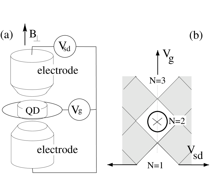
FIG. 1.: (a) Vertical Quantum Dot with contacts in a pillar configuration. (b) Grey-scale plot of the differential conductance $vs$ gate voltage $V_{g}$ and biasing voltage $V_{sd}$ (schematic), showing the CB regions (white) at various $N$. Operation point is marked by $\otimes$.

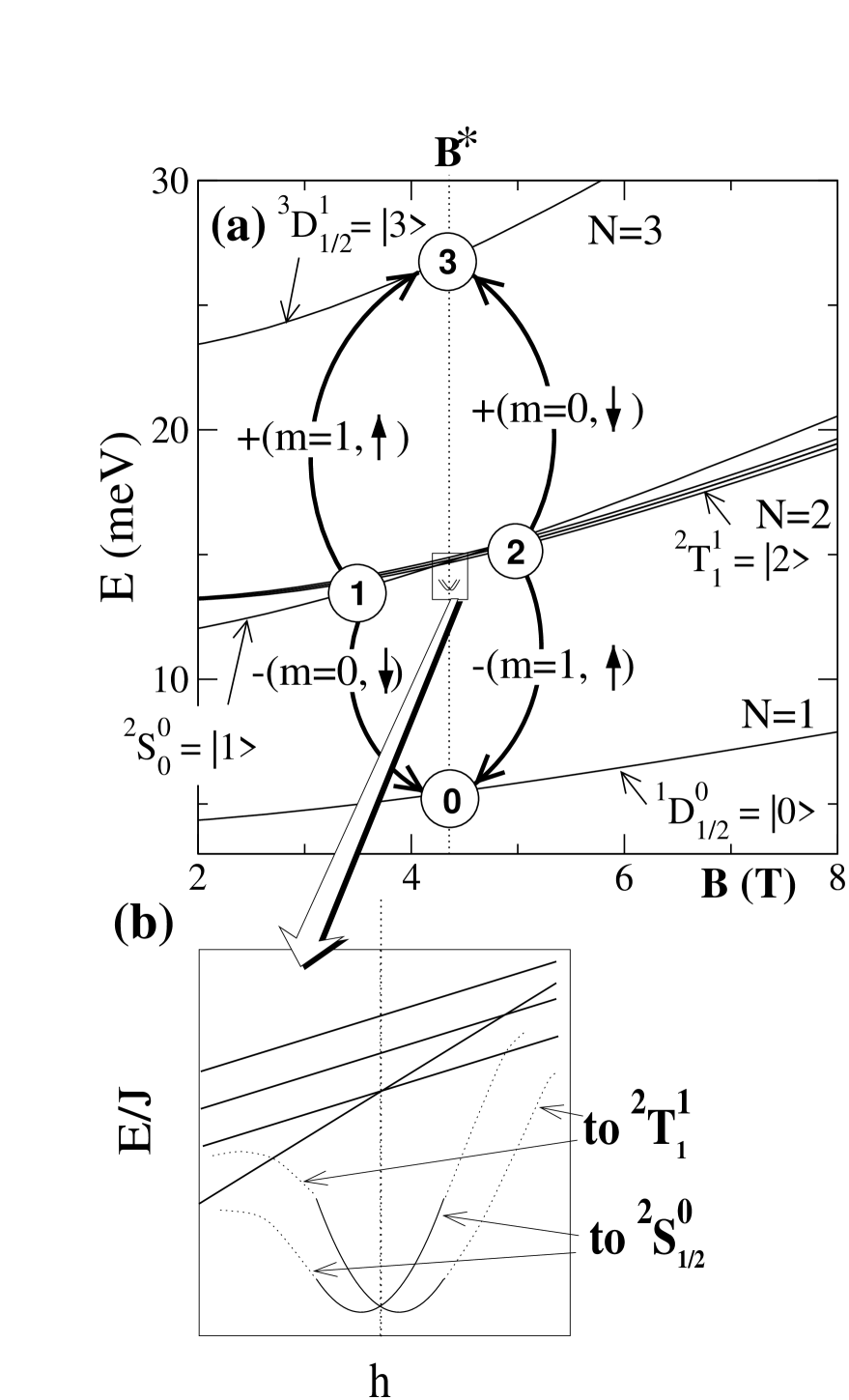
FIG. 2.: (a) General scheme of the energy level of the QD $vs$ magnetic field $B$. Only few states are plotted (labels are defined in Section II). The level spacing of the parabolic lateral confinement of the QD is $\hbar\omega_{0}$= 4meV , the Coulomb interaction $U$ = 3meV. Circled numbers represent the four dot states involved in the Kondo resonance. (b) Energy gain of the Kondo correlated state (not in scale) and removal of the degeneracy at $\delta B=B-B_{*}\neq 0$ ( $h\propto\delta B/T_{K}$: see Section V).

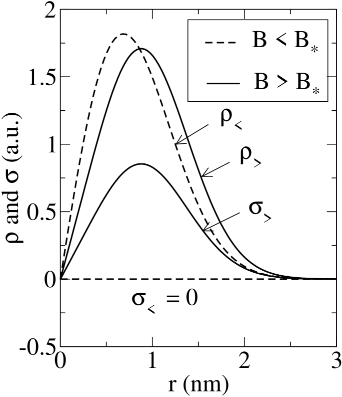
FIG. 3.: Charge density as a function of the radius $r$. $B<B_{*}$ ($B>B_{*}$) should be understood as $B$ slightly smaller (higher) than $B_{*}$. The charge density $\rho$ is only slightly affected when $B$ goes across $B_{*}$. The spin density $\sigma$ is zero when $B<B_{*}$. It has the profile of the charge density as $B>B_{*}$ ($\sigma_{>}=\frac{1}{2}\rho_{>}$).

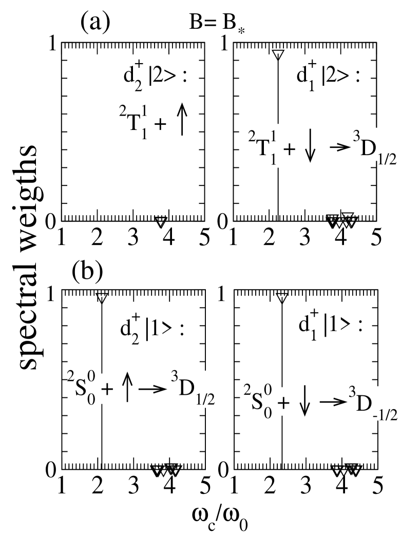
FIG. 4.: Spectral weights for addition of a spin up or down to the N=2 states. (a) Top panel-left: Spectral weight for addition of a $(m=1,\uparrow)$-spin electron to $~{}^{2}T_{1}^{1}$; -right: Spectral weight for addition of a $(m=0,\downarrow)$-spin electron. (b) Bottom panel-left: Spectral weight for addition of a $(m=1,\uparrow)$-spin electron to $~{}^{2}S_{0}^{0}$; -right: Spectral weight for addition of a $(m=0,\downarrow)$-spin electron. Separation of the peaks is due to the Zeeman spin splitting

REFERENCES

- [1] L.P. Kouwenhoven et al., in “Mesoscopic electron transport”, L. Sohn, L.P. Kouwenhoven and G. Schön eds., NATO ASI Series E 345,105; Kluwer, Dordrecht,Netherlands (1997).
- [2] L.P. Kouwenhoven et al. , Science 278, 1788 (1997); S. Tarucha et al., Phys. Rev. Lett. 77, 3613 (1996).
- [3] J. Schmid, J. Weis, K. Eberl and K.v. Klitzing, Physica B 256-258, 182 (1998).
- [4] D. Goldhaber-Gordon, H. Shtrikman, D. Mahalu, D. Abusch-Magder, U. Meirav and M.A. Kastner, Nature 391, 156 (1998).
- [5] S.M. Cronenwett, T.H. Oosterkamp and L.P. Kouwenhoven, Science 281, 540 (1998).
- [6] L.I. Glazman and M.E. Raikh, Pis’ma Zh. Eksp. Teor. Fiz. 47,378 (1988) [JETP Lett. 47,452 (1988)]; T.K.Ng and P.A.Lee, Phys. Rev. Lett. 61,1768 (1988); W. Xue and P.A. Lee, Phys. Rev. B 38,3913 (1988); Y. Meir, N.S. Wingreen and P.A. Lee, Phys. Rev. Lett. 70, 2601 (1993).
- [7] A.C. Hewson: “The Kondo Effect to Heavy Fermions” (Cambridge University Press, Cambridge, 1993).
- [8] S. Sasaki, S. De Franceschi, J.M. Elzerman, W.G. van der Wiel, M. Eto, S. Tarucha and L.P. Kouwenhoven, Nature 405, 764 (2000).
- [9] S. Tarucha, D.G. Austing, Y. Tokura, W.G. van der Wiel and L.P. Kouwenhoven, Phys. Rev. Lett. 84, 2485 (2000).
- [10] M. Eto and Y. Nazarov, Phys. Rev. Lett. 85, 1306 (2000).
- [11] M.Pustilnik and L.I.Glazman, Phys. Rev. Lett. 85, 2993 (2000).
- [12] M. Wagner, U. Merkt and A.V. Chaplik, Phys. Rev. B 45, 1951 (1992).
- [13] B. Jouault, G. Santoro and A. Tagliacozzo, Phys. Rev. B 61, 10242 (2000).
- [14] D. Giuliano and A. Tagliacozzo, Phys. Rev. Lett. 84, 4677 (2000).
- [15] a similar construction appears in [11] for the TS crossing point but there the role of the two fictious spins is quite different from the here.
- [16] a model has been proposed for the case when is parallel to the dot plane[17] which shows some similarities to ours at first sight. However it does not apply to the ST crossing as is discussed in Section VI.
- [17] M. Pustilnik, Y. Avishai and K. Kikoin, Phys. Rev. Lett. 84, 1756 (2000).
- [18] Yosida K., Phys. Rev. 147, 223 (1966); G.D.Mahan, “Many-Particle Physics” (New York : Plenum Press, 1990).
- [19] I. Affleck, Acta Phys. Pol. B 26, 1869 (1995).
- [20] A.M. Tsvelick and P.B. Wiegmann, Adv. Phys. 32,453 (1983). P.B. Wiegmann and A.M. Tsvelick, J. Phys. C, 2281 (1983); , 2321.
- [21] D.C. Mattis, Phys. Rev. Lett. 19, 1478 (1967); P. Nozières and A. Blandin, J. Physique 41, 193 (1980).
- [22] P.W. Anderson, J. Phys. C, 2436 (1970).
- [23] Note that with =8 meV and =6 meV used in B.Jouault et al. cond-mat/9810094, the S-T crossing takes place at 11T with a spin splitting of =0.27 meV. However, the amount of the splitting depends on the actual value of the effective giromagnetic factor which is controversial for dots ( M. Dobers, K.v. Klitzing and G. Weinmann, Phys. Rev B 38, 5453 (1988)).
- [24] D.R. Hamann, Phys. Rev. B 2, 1373 (1970); P.W. Anderson, G. Yuval and D.R. Haman, Phys. Rev. B 1, 4464 (1970).
- [25] L.A. Takhtajan and L.D. Fadeev, Russ. Math. Surveys 34, 11 (1979).
- [26] P.Noziéres, J. Low Temp. Phys. 17 31 (1974).
- [27] F. Gebhard and D. Vollhardt, Phys. Rev. Lett. 59, 1472 (1987).
- [28] For simplicity one electron per site will be implicitely assumed but this choice is inessential.
- [29] lifting of the degeneracy of the two variational states when electron-hole symmetry is broken is a feature in common with [18].
- [30] it would not be so in Yosida’s original approach.
- [31] note added in proof: this opinion also appears in the conclusions of ref.[11].
- [32] Yu.N. Ovchinnikov and A.M. Dyugaev, JETP Lett.s 70, 111 (1999); Yu.N. Ovchinnikov and A.M. Dyugaev, JETP 88, 696 (1999).
- [33] Our result fixes a sign mistake in ref.[17]. where is immediately apparent that the effective Hamiltonian, as it stands, is not spin-rotationally invariant in the limit in which couplings to states 1 and 2 are equal, thus leading to an unphysical result.