Large Stock Market Price Drawdowns Are Outliers

Abstract

Drawdowns (loss from the last local maximum to the next local minimum) offer a more natural measure of real market risks than the variance, the value-at-risk or other measures based on fixed time scale distributions of returns. Here, we extend considerably our previous analysis of drawdowns by analyzing the major financial indices, the major currencies, gold, the twenty largest U.S. companies in terms of capitalisation as well as nine others chosen randomly. Approximately $98\%$ of the distributions of drawdowns is well-represented by an exponential (or a minor modification of it with a slightly fatter tail), while the largest to the few ten largest drawdowns are occurring with a significantly larger rate than predicted by the exponential. This is confirmed by extensive testing on surrogate data. Very large drawdowns thus belong to a different class of their own and call for a specific amplification mechanism. Drawups (gain from the last local minimum to the next local maximum) exhibit a similar behavior in only about half the markets examined.

Large Stock Market Price Drawdowns Are Outliers

1 Introduction

It is now quite universally accepted that the distribution of asset returns is not only leptokurtotic but belongs to the class of fat tailed distributions. More formally, it has been shown that the tails of the distribution of returns follow approximately a power law $P({\rm return}>x)\sim C/x^{\mu}$, with estimates of the ’tail index’ $\mu$ falling in the range 2 to 4 [de Vries (1994); Lux (1996); Pagan (1996); Guillaume et al. (1997); Gopikrishnan et al. (1998)]. This implies that the second and probably the third moment of the distribution are finite. Extrapolating this distribution to infinite values, the fourth and higher moments are predicted to be mathematically infinite. This approximate law seems to hold for returns calculated over time scales ranging from a few minutes to about three weeks while the distributions are consistent with a slow convergence to Gaussian behavior at larger time scales [Gopikrishnan et al. (1998); Plerou et al. (1999)]. An alternative description with finite moments of all orders but still with fat tails has been suggested in terms of stretched exponential, also known as sub-exponential or Weibull (with exponent less than one) distributions [Laherrère and Sornette (1998)] (see [Sornette (2000)] for a synthesis of maximum likelihood estimators for the Weibull distributions).

This “one-point” statistics is however far from sufficient for characterizing market moves [Campbell et al. (1997); Lo and MacKinlay (1999)]. Two-point statistics, such as correlations of price returns and of volatilities (with the persistence phenomenon modeled by ARCH processes and its generalizations) offers important and complementary but still limited informations. In principle, one would like to have access to the full hierarchy of multiple-point correlations functions, but this is not attainable in practice due to finite statistics. A short-cut is to realize that using a fixed time scale, such as daily returns, is not adapted to the real dynamics of price moves and that relatively low-order statistics with suitable adjustments to the relevant time scales of the market may be more efficient descriptions. Indeed, physical time is probably not the proper quantity to characterize the flow of information and the rhythm of trading. Clark (1973) first noticed that subordinated processes, in which time is itself a stochastic process, provide a natural mechanism for fat tails resulting from the fact that the distribution of increments of subordinate random walks is a mixture of normal distributions (which is generically leptokurtic). A possible candidate for the stochastic time process (the subordinator) is the transaction volume [Clark (1973)] or the number of trades [Geman and Ané (1996)]. These processes can be generalized into multifractal subordinated processes [Mandelbrot (1997)]. In a similar vein, Müller et al. (1995), Guillaume et al. (1995) and Dacorogna et al. (1996) have advocated the concept of an elastic time that expands periods of high volatility and contracts those of low volatility, thus capturing better the relative importance of events on the market. Related empirical works have shown that return volatilities exhibit long-range correlations organized in a hierarchical way, from large time scales to small time scales [Ghashghaie et al. (1996); Müller et al. (1997); Dacorogna et al. (1998); Arneodo et al. (1998); Ballocchi et al. (1999); Muzy et al. (2000, 2001); Breymann et al. (2000)]. All these approaches suggest that a fixed time scale is not adequate for capturing the perception of risk and return experienced by traders and investors. There is thus a large potential gain in being time-adaptive rather than rigid in order to gain insight into the dynamics of financial markets.

Extreme value theory (EVT) provides an alternative approach, still based on the distribution of returns estimated at a fixed time scale. Its most practical implementation is based on the so-called “peak-over-threshold” distributions [Embrechts et al., 1997; Bassi et al., 1998], which is founded on a limit theorem known as the Gnedenko-Pickands-Balkema-de Haan theorem which gives a natural limit law for peak-over-threshold values in the form of the Generalized Pareto Distribution (GPD), a family of distributions with two parameters based on the Gumbel, Weibull and Frechet extreme value distributions. The GPD is either an exponential or has a power law tail. Peak-over-threshold distributions put the emphasis on the characterization of the tails of distribution of returns and have thus been scrutinized for their potential for risk assessment and management of large and extreme events (see for instance [Phoa, 1999; McNeil, 1999]). In particular, extreme value theory provides a general foundation for the estimation of the value-at-risk for very low-probability “extreme” events. There are however severe pitfalls [Diebold et al., 2001] in the use of extreme value distributions for risk management because of its reliance on the (unstable) estimation of tail probabilities. In addition, the EVT literature assumes independent returns, which implies that the degree of fatness in the tails decreases as the holding horizon lengthens (for the values of the exponents found empirically). Here, we show that this is not the case: returns exhibit strong correlations at special times precisely characterized by the occurrence of extreme events, the regime that EVT aims to describe. This suggests to re-examine EVT and extend it to variable time scales, for instance by analyzing the EVT of the distribution of drawdowns and drawups.

In order to address the problem of the possible effect of correlations that may occur at different time scales, we focus here on the statistics of drawdowns (and their complement, the drawups). We define a drawdown as a persistent decrease in the price (specifically the closing price) over consecutive days. A drawdown is thus the cumulative loss from the last maximum to the next minimum of the price. Symmetrically, a drawup is defined as the change (in percent) between a local minimum and the following maximum, i.e., a drawup is the event that follows the drawdown and vice versa. A drawup is a drawdown for an agent with a short (sell) position on the corresponding market.

Drawdowns are highly relevant: they measure directly the cumulative loss that an investment can incur. They also quantify the worst case scenario of an investor buying at the local high and selling at the next minimum. It is thus worthwhile to ask if there is any structure in the distribution of drawdowns. Notice that drawdowns embody a subtle dependence since they are constructed from runs of the same sign variations. They are not defined over a fixed time scale. Some drawdowns will last only one day, other five days or more. Their distribution measures how successive drops can influence each other and construct a persistent process, not captured by the distribution of returns nor by the two-point correlation function. In Appendix A, we show that the distribution of drawdowns for independent price increments $x$ is asymptotically an exponential (while the body of the distribution is Gaussian [Mood (1940)]) when the distribution of $x$ does not decay more slowly than an exponential, i.e., belong to the class of exponential or super-exponential distributions. In contrast, for sub-exponentials (such as stable Lévy laws, power laws and stretched exponentials), the tail of the distribution of drawdowns is asymptotically the same as the distribution of the individual price variations. Since stretched exponentials have been found to offer an accurate quantification of price variations [Lahérrere and Sornette, 1998; Sornette et al., 2000; Andersen and Sornette, 2001] thus capturing a possible sub-exponential behavior and since they contain the exponential law as a special case (exponent $z=1$ in the definition (4)), we shall take the stretched exponential law as our null hypothesis.

Our emphasis on drawdowns is motivated by two considerations: 1) drawdowns are important measures of risks used by practitioners because they represent their cumulative loss since the last estimation of their wealth. It is indeed a common psychological trait of people to estimate a loss by comparison with the latest maximum wealth; 2) drawdowns automatically capture an important part of the time dependence of price returns, similarly to the so-called run-statistics often used in statistical testing [Knuth (1969)] and econometrics [Campbell et al. (1997); Barber and Lyon (1997)]. As we have previously showed [Johansen and Sornette (1998,2000b)], the distribution of drawdowns contains an information which is quite different from the distribution of returns over a fixed time scale. In particular, a drawndown embodies the interplay between a series of losses and hence measures a “memory” of the market. Drawdowns will examplify the effect of correlations in price variations when they appear, which must be taken into account for a correct characterisation of market price variations. They are direct measures of a possible amplification or “flight of fear” where previous losses lead to further selling, strengthening the downward trend, occasionally ending in a crash. We stress that drawdowns, by the “elastic” time-scale used to define them, are effectively function of several higher order correlations at the same time.

The data used in our work comprises

1. major world financial indices: the Dow Jones, Standard & Poor, Nasdaq Composite, TSE 300 Composite (Toronto, Canada), All Ordinaries (Sydney stock exchange, Australia), Strait Times (Singapore stock exchange), Hang Seng (Hong Kong stock exchange), Nikkei 225 (Tokyo stock exchange, Japan), FTSE 100 (London stock exchange, U.K.), CAC40 (Paris stock exchange, France), DAX (Frankfurt stock exchange, Germany), MIBTel (Milan stock exchange, Italy);

2. currencies: US$/DM, US$/Yen, US$/CHF;

3. gold;

4. the $20$ largest companies in the US market in terms of capitalisation, as well as 9 others taken randomly in the list of the 50 largest companies (Coca Cola, Qualcomm, Appl. Materials, Procter&Gamble, JDS Uniphase, General Motors, Am. Home. Prod., Medtronic and Ford).

These different data have not the same time span, largely due to different lifespan, especially for some recent “new technology” companies. In this selection of time series, we are far from exhaustive but have a reasonable sample for our purpose: as we shall see, with the exception of the index CAC40 (the “French exception”?), all time series 1-3 exhibit clear outlier drawdowns. This suggests that outliers constitute an ubiquitous feature of stock markets, independently of their nature.

In the next section 2, we discuss some properties of drawdowns. In particular, we analyze the drawdowns of a model with no correlation but strong dependence and present preliminary evidence of intermittent dependence on the Dow Jones Industrial Average index.

In section 3, we present our results for the drawdowns and the drawups of the major world financial markets, of the major world currencies and of gold. While it is well-known that price returns are essentially uncorrelated, section 3 will show that strong correlations do appear at special times when large drawdowns and drawups occur: the distribution of large drawdowns and large drawups is strongly non-exponential with a much fatter tail. Since this anomalous behavior is observed only for the largest drawdowns and drawups, in some cases up to a few tens of the largest events, these very large drawdowns and drawups can thus be considered to be outliers because they do not conform to the model suggested by the main part of the data. This points to the brief appearence of a dependence in successive drops leading to an amplification which makes these drops special. The results confirm and extend our previous announcements [Johansen and Sornette (1998,2000b)]. We test these results by constructing error plots and by adding noise to investigate the robustness of the distribution of drawdowns and drawups.

Section 4 presents the evidence that large drawdowns and drawups are outliers for 29 of the largest US companies. The distribution of drawups is found significantly different from that of drawdowns. While drawups of amplitude larger than $15\%$ occur about twice as often as drawdowns of the same amplitude, the case for the largest drawups to be outliers is less clear-cut. Half the time series have their largest drawups significantly larger than explained by the bulk of the distribution, the converse is observed for the other half. It thus seems that outlier drawups is a less conspicuous feature of financial series with more industry specificities than the ubiquitous outlier drawdowns observed essentially in all markets.

Section 5 presents statistical tests using surrogate data that confirm that large drawdowns are outliers with a large degree of significance.

Section 6 summarizes our results and concludes with a discussion on the implications for risk management.

Appendix A derives the distribution of drawdowns for a large class of distributions of returns in the restricted case of independent returns. The results justify our choice of the exponential and stretched exponential null hypothesis. Appendix B gives the confidence interval for drawdowns when the distribution of returns is in the exponential or superexponential class.

2 Some properties of drawdowns

2.1 A model with no correlation but strong dependence

To see how subtle dependences in successive price variations are measured by drawdowns, consider the simple but illustrative toy model in which the price increments $\delta p(t)$ are given by [Robinson (1979); Hsieh (1989)]

$$\delta p(t)=\epsilon(t)+\epsilon(t-1)\epsilon(t-2)~{},$$ (1)

where $\epsilon(t)$ is a white noise process with zero mean and unit variance. Then, the expectation ${\rm E}(\delta p(t))$ as well as the two-point correlation ${\rm E}(\delta p(t)\delta p(t^{\prime}))$ for $t\neq t^{\prime}$ are zero and $\delta p(t)$ is also a white noise process. However, the three-point correlation function ${\rm E}(\delta p(t-2)\delta p(t-1)\delta p(t))$ is non-zero and equal to $1$ and the expectation of $\delta p(t)$ conditioned on the knowledge of the two previous increments $\delta p(t-2)$ and $\delta p(t-1)$ is non-zero and equal to

$${\rm E}(\delta p(t)|\delta p(t-2),\delta p(t-1))=\delta p(t-2)\delta p(t-1)~{},$$ (2)

showing a clear predictive power. This leads to a very distinct signature in the distribution of drawdowns. To simplify the analysis to the extreme and make the message very clear, let us restrict to the case where $\epsilon(t)$ can only take two values $\pm 1$, Then, $\delta p(t)$ can take only three values $0$ and $\pm 2$ with the correspondance

$$\epsilon(t-2),\epsilon(t-1),\epsilon(t)~{}~{}~{}~{}~{} \to ~{}~{}~{}~{}~{}\delta p(t)$$ (3)

$$+++~{}~{}~{}~{}~{} \to ~{}~{}~{}~{}~{}+2$$

$$++-~{}~{}~{}~{}~{} \to ~{}~{}~{}~{}~{}0$$

$$+-+~{}~{}~{}~{}~{} \to ~{}~{}~{}~{}~{}0$$

$$+--~{}~{}~{}~{}~{} \to ~{}~{}~{}~{}~{}-2$$

$$-++~{}~{}~{}~{}~{} \to ~{}~{}~{}~{}~{}0$$

$$-+-~{}~{}~{}~{}~{} \to ~{}~{}~{}~{}~{}-2$$

$$--+~{}~{}~{}~{}~{} \to ~{}~{}~{}~{}~{}+2$$

$$---~{}~{}~{}~{}~{} \to ~{}~{}~{}~{}~{}0$$

where the left colum gives the three consecutive values $\epsilon(t-2),\epsilon(t-1),\epsilon(t)$ and the right column is the corresponding price increment $\delta p(t)$. We see directly by this explicit construction that $\delta p(t)$ is a white noise process. However, there is a clear predictability and the distribution of drawdowns reflects it: there are no drawdowns of duration larger than two time steps. Indeed, the worst possible drawdown corresponds to the following sequence for $\epsilon$: $--+--$. This corresponds to the sequence of price increments $+2,-2,-2$, which is either stopped by a $+2$ if the next $\epsilon$ is $+$ or by a sequence of $0$’s interupted by a $+2$ at the first $\epsilon=+$. While the drawdowns of the process $\epsilon(t)$ can in principle be of infinite duration, the drawdowns of $p(t)$ cannot. This shows that the structure of the process $\delta p(t)$ defined by (1) has a dramatic signature in the distribution of drawdowns in $p(t)$ and illustrates that drawdowns, rather than daily or weekly returns or any other fixed time scale returns, are useful time-elastic measures of price moves.

2.2 Variations on drawdowns

There is not a unique definition of drawdowns as there are several possible choices for the peak where the drawdown starts from. For instance, the “current drawdown” is the amount in percent that a portfolio has declined from its most recent peak. The maximum drawdown is the largest amount (in percent) that a fund or portfolio dropped from a peak over its lifetime. Grossman and Zhou (1993) analyze the optimal risky investment for an investor not willing to lose at each point in time a drawdown (calculated relative to the highest value of the asset in the past) larger than a fixed percentage of the maximum value his wealth has achieved up to that time. Maslov and Zhang (1999) have investigated the distribution of “drawdowns from the maximum”, where the drawdowns are also calculated relative to the highest value of the asset in the past. This distribution is defined only for an asset exhibiting a long-term upward trend and can be shown, for uncorrelated returns, to lead to power law distributions. In this paper, drawdowns will be defined as the decrease in percent from a local maximum to the following local minimum after which the price again increases.

2.3 Preliminary evidence of intermittent dependence

Appendix A shows that the distribution of drawdowns for independent price increments $x$ is asymptotically an exponential when the distribution of $x$ does not decay more slowly than an exponential, i.e., belong to the class of exponential or super-exponential distributions. In contrast, for sub-exponentials (such as stable Lévy laws, power laws and stretched exponentials), the tail of the distribution of drawdowns is found to be asymptotically the same as the distribution of the individual price variations.

These results hold as long as the assumption, that successive price variations are uncorrelated, is a good approximation. There is a large body of evidence for the correctness of this assumption for the largest fraction of trading days [Campbell et al. (1997)]. However, consider, for instance, the 14 largest drawdowns that has occurred in the Dow Jones Industrial Average in the last century. Their characteristics are presented in table 1. Only 3 lasted one or two days, whereas 9 lasted four days or more. Let us examine in particular the largest drawdown. It started on Oct. 14, 1987 (1987.786 in decimal years), lasted four days and led to a total loss of $-30.7\%$. This crash is thus a run of four consecutive losses: first day the index is down with $3.8\%$, second day with $6.1\%$, third day with $10.4\%$ and fourth with $30.7\%$. In terms of consecutive losses this correspond to the following sequence of daily losses: $3.8\%$, $2.4\%$, $4.6\%$ and $22.6\%$ on what is known as the Black Monday of 19th Oct. 1987.

The observation of large successive drops is suggestive of the existence of a transient correlation. To make this point clear, consider an hypothetical drawdown of $30\%$ made up of three successive drops of $10\%$ each. A daily loss of $10\%$, while severe, is not that uncommon and occurs typically once every four years (or one in about $1000$ trading days). It thus corresponds to a probability of $10^{-3}$. Assuming that the three successive drops of $10\%$ are uncorrelated, the probability of the drawdown of $30\%$ is $[10^{-3}]^{3}=10^{-9}$, i.e., corresponds to one event in four millions years. In other words, the lack of correlations is completely in contradiction with empirical observations.

For the Dow Jones, this reasoning can be adapted as follows. We use a simple functional form for the distribution of daily losses, namely an exponential distribution with decay rate $1/0.63\%$ obtained by a least-square fit. This quality of the exponential model is confirmed by the direct calculation of the average loss amplitude equal to $0.67\%$ and of its standard deviation equal to $0.61\%$ (recall that an exact exponential would give the three values exactly equal). Using these numerical values, the probability for a drop equal to or larger than $3.8\%$ is $\exp(-3.8/0.63)=2.4~{}10^{-3}$ (an event occurring about once every two years); the probability for a drop equal to or larger than $2.4\%$ is $\exp(-2.4/0.63)=2.2~{}10^{-2}$ (an event occurring about once every two months); the probability for a drop equal to or larger than $4.6\%$ is $\exp(-4.6/0.63)=6.7~{}10^{-4}$ (an event occurring about once every six years). Under the hypothesis that these three first events are uncorrelated, they together correspond to a probability of occurrence of $3.5~{}10^{-8}$, i.e., one event in about $11,000$ years, an extremely rare possibility. It turned out that, not only this exceedingly rare drawdown occurred in Oct. 1987 but, it was followed by an even rarer event, a single day drop of $22.6\%$. The probability for such a drop equal to or larger than $22.6\%$ is $\exp(-22.6/0.63)=2.6~{}10^{-16}$ (an event occurring about once every $10^{14}$ years). All together, under the hypothesis that daily losses are uncorrelated from one day to the next, the sequence of four drops making the largest drawdown occurs with a probability $10^{-23}$, i.e., once in about $4$ thousands of billions of billions years. This clearly suggests that the hypothesis of uncorrelated daily returns is to be rejected and that drawdowns and especially the large ones may exhibit intermittent correlations in the asset price time series.

3 Cumulative distributions of drawdowns and drawups for major world indices, currencies and gold

In this section, we present three pieces of evidence supporting the existence of two classes of drawdowns (and to a lesser degree of drawups).

First for all studied assets, we construct on the same graphs the cumulative distribution of drawdowns and the complementary cumulative distribution of drawups. Each of these cumulative distributions is fitted to the null hypothesis taken as an exponential or a stretched exponential represented in the graphs by the continuous lines. The cumulative stretched distribution is defined by

$$N_{c}\left(x\right)=A~{}\exp\left(-(|x|/\chi)^{z}\right)~{},$$ (4)

where $x$ is either a drawdown or a drawup. In order to stabilize the fit, it has been performed as $\log(N_{c})=\log(A)-B|x|^{z}$, where $A$ is the total number of drawdowns (or drawups) and hence is fixed . The characteristic scale $\chi$ is related to the coefficient $B$ by the relation $\chi=1/B^{1/z}$. When $z<1$ (resp. $z>1$), $N_{c}\left(x\right)$ is a stretched exponential or sub-exponential (resp. super-exponential). The special case $z=1$ corresponds to a pure exponential. In this case, $\chi$ is nothing but the standard deviation of $|x|$.

The success in using the stretched exponential for parameterising the data does not of course mean that better parametrizations cannot be found, neither does it prove that the processes governing the dynamics of the main part of the distribution is giving stretched exponential distributions. As we said above, its virtue lies in the fact that it is a straightforward generalisation of the pure exponential, which represents the simplest and natural null-hypothesis for uncorrelated price variations. We find that the stretched exponential model parameterizes $\approx 98\%$ of all data points, while the $2\%$ largest values are the “outliers”. We find that twelve markets have a value of the exponent $z$ below $1$ and only five have a value larger than $1$.

The second piece of evidence is provided by plotting the relative error between the empirical cumulative distributions and the stretched exponential fits. This graphical presentation makes very apparent the transition between the two regimes.

Third, we test for the robustness of these results by adding noise of different amplitudes to the data.

3.1 Major financial indices

Figures 1 to 3 show the cumulative distributions $N_{c}\left(x\right)$ of drawdowns and complementary distributions of drawups in three major US indices: The Dow Jones Industrial Average, the S&P500 and the Nasdaq Composite. The two continuous lines show the fits of these two distributions with the stretched exponential distribution defined by formula (4). Up to drawdawns of amplitudes $\approx 10\%$, the stretched exponential distribution provides a faithful description while above $\approx 10\%$, the distribution “breaks away”, most abruptly for the Dow Jones Industrial Average and the S&P500.

Both the Dow Jones Industrial Average and the Nasdaq Composite indice show a distinct upward curvature in the distribution of drawdowns corresponding to $z\approx 0.82\pm 0.02$, whereas the S&P500 is closer to a pure exponential with $z\approx 0.90$, see table 2. Note that an exponent $z<1$ corresponds to a fatter tail than an exponential. The law (4) is also known in the mathematical literature as a “subexponential” and in the engineering field as a stretched distribution (see chap. 6 in (Sornette, 2000) for useful informations on this family of distributions and how to calibrate them). Our aim is not to defend the model (4) but rather to use it as a convenient and parsimonious tool. This family (4) is particularly adapted to our problem because it both contains the null hypothesis of an exponential distribution $z=1$ valid for exponential and superexponential distributions and also allows us to describe subexponential distributions (see Appendix A). Allowing $z$ to depart from $1$ then provides us a simple and robust measure of the deviation from an exponential. We actually find that allowing for an even fatter tail is not enough to account for the very largest drawdowns which wildly depart from this description. Playing the devil’s advocate, one could argue that the strong departure from model (4) of the few largest drawdowns observed in figures 1 to 3 is not a proof of the existence of outliers, only of the inadequacy of the model (4). It is true that we can never prove the existence of outliers in an absolute sense. However, we have calculated a reasonable null-hypothesis, provided a family of distributions that extends the null-hypothesis to account for larger moves. Nevertheless, we find that the largest drawdowns are utterly different from the distribution containing approximately $98\%$ of the data. We find this to be an important message which may lead to a better understanding of how the financial markets react in times of large losses. This has been tested within a rigorous statistical procedure in [Sornette and Johansen, 2001].

There is a clear asymmetry between drawdowns and drawups. The asymmetry occurs more clearly in the bulk of the distribution for the Dow Jones Industrial Average where $z=0.84\pm 0.01$ for drawdowns compared to $z=0.99\pm 0.01$ for drawups. In the case of the Dow Jones Industrial Average, the change of regime to extreme events is maybe even stronger for drawups than for drawdowns. The difference is weaker for the S&P500 index with $z=0.90\pm 0.01$ for drawdowns compared to $z=1.03\pm 0.02$ for drawups. The change of regime occurs clearly for both drawdowns and drawups with the difference that a very strong outlier exists only for drawdowns. The asymmetry in the bulk of the distributions of drawdowns and drawups is also apparent for the Nasdaq composite index with $z=0.80\pm 0.02$ for drawdowns compared to $z=0.90\pm 0.02$ for drawups. However, the asymmetry is much more pronounced in the extreme event regime: no clear change of regime is observed for drawups whose full distribution is satisfactory described by the stretched exponential distribution (4) while a strong departure from (4) is observed for the five large drawdowns.

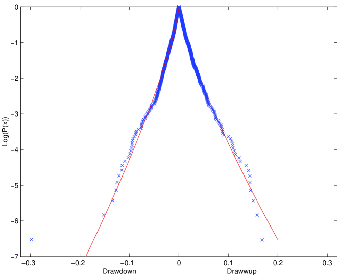
Figure 6: Same as figure 1 for the Strait Times index (Singapore stock exchange).

Is this behavior confined to U.S. markets or is it a more general feature of stock market behavior? In order to answer this question, we have analysed the main stock market index of the remaining six G7-countries as well as that of Australia, Hong-Kong and Singapore. The results of this analysis is shown in figures 4 to 12 and more quantitatively in table 2. Quite remarkably, for the drawdowns, we find that all markets except the French market, the Japanese market being on the borderline, show the same qualitative behavior exhibiting a change of regime and the presence of “outliers”. The Paris stock exchange is the only exception as the distribution of drawdowns is an almost perfect exponential. It may be that the observation time used for CAC40 is not large enough for an outlier to have occurred. If we compare with the Strait Times index (Singapore stock exchange) shown in figure 6, we see that all the distribution except the single largest drawdown is very well-fitted by a stretched exponential. The presence or absence of this outlier thus makes all the difference.

The results obtained for the drawups are not as clear-cut as for the drawdowns. Whereas the distributions for the Dow Jones Industrial Average and the S&P500 clearly exhibits a similar behavior to that of the drawdowns, this is not the case for the TSE 300, the Strait times, the Hang Seng, the FTSE 100, the DAX and the MIBTel indices. The other markets are at the borderline of significance. In the one case where we have sufficient statistics (for the Dow Jones Industrial Average), we have successfully parameterized the tail of the drawup distribution with another stretched exponential (not shown), see table 3. However, how to interpret the interpolation of such two rather excellent fits is difficult. With respect to the other markets that clearly exhibit outliers, it is impossible to give a qualified estimation of the distribution of the outliers due to the limited statistics just as with the drawdowns.

To quantify the statistical significance of the fluctuations obtained in the exponent $z$ reported in table 2, we use the asymptotic covariance matrix of the estimated parameters, the typical scale $\chi\equiv 1/B^{1/z}$ and the exponent $z$ calculated by Thoman et al. (1970):

$${\sigma_{\chi}\over\chi} = {1.053\over z}~{}{1\over\sqrt{N}}~{},$$ (5)

$${\sigma_{z}\over z} = {0.78\over\sqrt{N}}~{},$$ (6)

where $N$ is the sample size (number of drawdowns (resp. drawups) in our data sets) and $\sigma_{\chi}$ (resp. $\sigma_{z}$) is the standard deviation of $\chi$ (resp. $z$). The fluctuations in the exponent $z$ are statistically significant: excluding the CAC40, we find an average $z=0.87$ with a standard deviation of $0.04$ which is about two times larger than expected from the statistics (6). These two expressions (5) and (6) are used to give the one-sigma error bars in the tables.

3.2 Gold and in currencies

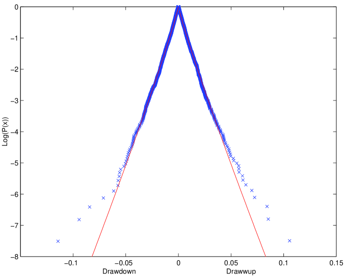
Figure 13: Same as figure 1 for the US$/DM exchange rate, i.e., US $ expressed in Deutchmark).

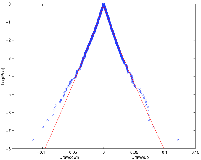
Figure 15: Same as figure 1 for the US$/CHF exchange rate i.e., US $ expressed in Swiss franc).

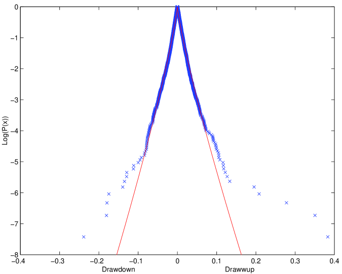
Figure 16: Same as figure 1 for Gold.

To test whether the existence of outliers beyond a stretched exponential regime apply more generally, we now analyze currencies and gold. As seen in figure 13 for the US$/DM exchange rate, figure 14 for the US$/YEN exchange rate, figure 15 for the US$/CHF exchange rate and figure 16 for gold, a similar behavior is observed. The exponent $z$ for drawdowns tends to be larger with a smaller characteristic drawdown $\chi$ (thinner tails) for currencies compared to the indices. The gold market and the currencies confirm the previous evidence by providing us with some of the strongest cases for the presence of outliers, together with the US indices, TSE 300, All Ordinaries, FTSE 100 and the DAX indices.

The bulk of the distributions of drawdowns and drawups are well-fitted by the stretched exponential model with an almost perfect symmetry except for the US$/YEN exchange rate. Indeed, the exponents $z$ and characteric scales $\chi$ are basically identical for drawdowns and drawups, except for the US$/YEN exchange rate which exhibits a strong asymmetry in the parameter $\chi=1.17\pm 0.03$ for drawdowns and $\chi=0.79\pm 0.02$ for drawups, while $z=0.90\pm 0.02$ is the same for both drawdowns and drawups. Interestingly, the asymmetry is further strengthened by the fact that the “outlier” regime is only observed for drawdowns while all the drawups are very well-described by the stretched exponential distribution, as seen in figure 14.

In general, it is expected that, for most currency pairs, the pdf for the return is symmetric. We note however that this is not always true: Laherrère and Sornette [1998] documented that the distribution of returns of the French franc expressed in German mark (before the introduction of the Euro) is asymmetric with a fatter tail for the losses than for the gains. Thus, the slow and continuous depreciation of the French franc against the German mark over the years preceding the unique European currency has occurred by a globally fatter distribution of losses rather than by a slow drift superimposed upon a symmetric distribution. It seems that a similar asymmetry of the daily return distribution of the US $ expressed in Yen may explain in part the asymmetry of the drawdowns: from 1972 to 1999, the US $ has lost a factor $3$ in its value compared to the Yen. As for the French franc/German mark case, this loss has occurred by a slighly fatter tail of the distribution of losses compared to the distribution of gains of the US $ in Yen. The construction of drawdowns seems to enhance this asymmetry of the distribution of daily returns and indicates that the slow depreciation of the US $ has occurred in bursts rather as a continuous drift. To investigate further this question, we analyzed the the GPB/US$ exchange rate and the GPB/DM distributions. We find that they are to a good approximation described by a pure exponential behaviour with no outliers. This may be the evidence of a singular increasing role played by the Japanese Yen over the thirty years since the early 1970s.

3.3 Error plots

Figures 17 and 18 show the differences (error plots) between the cumulative distributions of drawdowns (respectively drawups) and the best fits with the stretched exponential model (4) for the DJIA, the S&P500, the Nasdaq composite index, the German mark in US $ and Gold. These two figures clearly identify two regimes.

1. The bulk of the distributions correspond to errors fluctuating around $0$. This characterizes typically the drawdowns and drawups less than about $5-7\%$ representing about $98\%$ of the data points. This is nothing but a restatement of the good fit provided by the stretched exponential model.

2. In contrast, for drawdowns and drawups larger than $5-7\%$, one observes a striking systematic deviation characterizing the “outlier” regime.

3.4 Tests of robustness by adding noise

As we already mentioned, the definition of drawdowns and drawups may vary slightly under small changes in the data. For instance, consider a run of daily losses in which one day witnessed a small loss of $-0.05\%$. Had the market changed this value to a small gain of $+0.05\%$, this drawdown would have been replaced by two drawdowns separated by one slightly positive day. Since one should not expect such days with very small positive or negative returns to play a role in the significance of the cumulative losses and gains captured by the drawdowns, the question therefore arises whether our results are robust with respect to the addition of a noise that may modify these small returns.

In order to address this question, we define the “time series neighborhood” of a given price trajectory as follows.

1. We define the $i$-th return $r(i)=\ln[{\rm price}(i)]-\ln[{\rm price}(i-1)]$.

2. We perform the transformation $r(i)\to r_{A}(i)=r(i)+A~{}{\rm Ran}~{}\sigma$ where ${\rm Ran}$ is a i.i.d. random noise with uniform distribution in $[-1,+1]$ and $\sigma$ is the standard deviation of the returns. We have performed tests with $A=0$ (no added noise), $A=0.5,1$ and $2$.

3. We exponentiate the time series $r_{A}(i)$ to get a new noisy price time series

   $$p_{A}(i)=p_{0}\exp\left[r_{A}(i)+r_{A}(i-1)+r_{A}(i-2)+...+r_{A}(1)\right]~{}.$$ (7)

4. We then construct the runs of successive losses (drawdowns) and of successive gains (drawups) for this noise price time series $p_{A}(i)$.

If the anomalous behavior of the drawdowns in the “outlier” regime is due to high order correlations of the return, it should not be destroyed by the addition of noise and the distribution of outliers should be similar to the one computed with the initial price series. This is indeed verified in figures 19-21 which show the cumulative distribution of drawdowns and complementary distributions of drawups for the “time series neighborhoods” of the DJIA, the S&P500 and the Nasdaq composite index for the different values of $A=0$, $A=0.5,1$ and $2$.

These tests are encouraging. Other tests that will be reported elsewhere [Johansen and Sornette, in preparation] confirm this picture. They involve either ignoring increases (decreases) of a certain fixed magnitude (absolute or relative to the price) or ignorings increases (decreases) over a fixed time horizon and in both cases letting the drawdown (drawup) continue. Both approaches provide a natural “coarse-graining” of the drawdowns and drawups and confirm/strengthen the validity of our results.

4 Drawdowns and drawups in stock market prices of major US companies

4.1 “Universal” normalized distributions

We now extend our analysis to the very largest companies in the U.S.A. in terms of capitalisation (market value). The ranking is that of Forbes at the beginning of the year 2000. We have chosen the top 20, and in addition a random sample of other companies, namely number 25 (Coca Cola), number 30 (Oualcomm), number 35 (Appl. Materials), number 39 (JDS Uniphase), number 46 (Am. Home Prod.) and number 50 (Medtronic). Three more companies have been added in order to get longer time series as well as representatives for the automobile sector. These are Procter & Gamble (number 38), General Motors (number 43) and Ford (number 64). This represent a non-biased selection based on objective criteria.

To avoid a tedious repetition of many figures, we group the cumulative distributions of drawdowns and complementary cumulative distributions of all these stocks in the same figure 22. In order to construct this figure, we have fitted the stretched exponential model (4) to each distribution and obtained the corresponding parameters $A$, $\chi$ and $z$ given in tables 4 and 5. We then construct the normalized distributions

$$N_{C}^{(n)}(x)=N_{c}\left((|x|/\chi)^{z}\right)/A$$ (8)

using the triplet $A$, $\chi$ and $z$ which is specific to each distribution. Figure 22 plots the expression (8) for each distribution, i.e., $N_{c}/A$ as a function of $y\equiv{\rm sign}(x)~{}(x/\chi)^{z}$. If the stretched exponential model (4) held true for all the drawdowns and all the drawups, all the normalized distributions should collapse exactly onto the “universal” functions $e^{y}$ for the drawdowns and $e^{-y}$ for the drawups. We observe that this is the case for values of $|y|$ up to about $5$, i.e., up to typically $5$ standard deviations (since most exponents $z$ are close to $1$ as seen in tables 4 and 5), beyond which there is a clear upward departure observed both for drawdowns and for drawups. Comparing with the extrapolation of the normalized stretched exponential model $e^{-|y|}$, the empirical normalized distributions give about $10$ times too many drawdowns and drawups larger than $|y|=10$ standard deviations and more the $10^{4}$ too many drawdowns and drawups larger than $|y|=20$ standard deviations. Note that for AT&T, a crash of $\approx 73\%$ occurred which lies beyond the range shown in figure 22.

4.2 Detailed results on the distributions of drawdowns and drawups

A detailed analysis of each individual price distribution of drawdowns shows that the five largest companies (MicroSoft, Cisco, General Electric, Intel and Exxon-Mobil) clearly exhibits the same features as those for the major financial markets. Of the remaining 24, for all but America Online and JDS Uniphase, we find clear outliers but also a variety of different tails of the distributions. The main difference is in the value of the exponent $z$, which is $\approx 1$ or larger. This means that the distributions tends to bend downward instead of upward, thus emphasising the appearance the outliers. It is interesting to note that the two companies, America Online and JDS Uniphase, whose distributions did not exhibit outliers are also the two companies with by far the largest number per year of drawdowns of amplitude above $15\%$ (close to $4$), see table 4.

For the drawups in the price of major US companies, the picture is less striking when compared to the major financial markets. Again, a fraction of the companies exhibit a behavior similar to that of the major financial markets. A clear-cut distinction is always difficult, but we find three groups according to the outlier criterion:

• Obvious outliers: General Electric, Intel, Exxon-Mobil, Oracle, Wall-Mart, IBM, HP, Sun Microsystems, SBC, Coca-Cola, Procter & Gamble and Medtronic.

• Difficult to classify in the first group : AT&T, Citigroup, Applied Materials and General Motors.

• Clearly no outliers: Microsoft, Cisco, Lucent, Texas Instrument, Merck, EMC, Pifzer, AOL, MCI WorldComm., Qualkomm, JDS Uniphase, American Home Products and Ford.

This means that $12$ companies belong to the first catagory, $13$ to the last and only $4$ companies on the borderline. Hence, it is difficult to conclude with the same force as for the drawdowns about the existence of outliers. The concept of large drawups as outliers seems however a persuasive feature of about half the markets. Another interesting observation is that the fits with the stretched exponential are consistent with a value for the exponent $z\approx 1$ (albeit with significant fluctuations from market to market). The two observations may be related. Again, it is interesting to observe that the two companies, America Online and JDS Uniphase, which have by far the highest rate of drawdowns above $15\%$ also have by far the highest rate of drawups above $15\%$, as shown in table 5. In fact, this ranking holds approximately for most of the companies. Figure 23 shows the number of drawups of amplitude larger than $15\%$ as a function of the number of drawdowns larger than $15\%$ for all the companies analyzed here and shown respectively in tables 5 and 4. The linear regression is good with a $R$-statistics of $0.97$ and a correlation coefficient of $0.62$. In the linear regression, we have allowed the value $M1$ at the origin to be non-zero. However, the fit finds $M1$ to have a negligible value: vanishing draw downs come with vanishing draw ups.

Quantitatively, there are on average $0.94$ drawdowns per year per company of amplitude equal to or larger than $15\%$, compared to $1.92$ drawups per year per company of amplitude equal to or larger than $15\%$. Large drawups are twice as frequent and thus to a much lesser extent to be characterised as outliers. The difference cannot be attributed to a difference in the size of the two sets. It may be related to the very different value given to them by the market: drawups are cheered upon by the market and the media, whereas drawdowns are not considered well. Hence, both from the point of view of risk management and of market psychology, there is a strong asymmetry between drawups and drawdowns.

5 Synthetic tests and statistical significance

To further establish the statistical confidence with which we can conclude that the largest drawdowns are outliers, for each financial time series, we have reshuffled the daily returns 1000 times and hence generated 1000 synthetic data sets for each. This procedure means that 1000 synthetic data will have exactly the same distribution of daily returns as each time series. However, higher order correlations apparently present in the largest drawdowns are destroyed by the reshuffling. This surrogate data analysis of the distribution of drawdowns has the advantage of being non-parametric, i.e., independent of the quality of fits with a model such as the stretched exponential.

In order to compare the distribution of drawdowns obtained for the real data and for the synthetic data for each of the indices, of the currencies and of companies named in the first column of tables 6 and 7, a threshold given by the second column has been chosen by identifying the point of breakdown from the stretched exponential, i.e., the crossover point from bulk to outliers: the first point after this crossover point is then the smallest outlier and the threshold is the integer value of that drawdown. The third column gives the number of drawdowns above the threshold in the true data. The fourth column gives the number of surrogate data sets with $0,1,2,3,...$ drawdowns larger than the threshold. The last column quantifies the corresponding confidence level.

The results for the financial market indices, for the currencies and for gold exhibit a very high statistical confidence level about $99\%$, as shown in table 6. The situation is more dispersed for companies as shown in table 7: out of the $25$ companies presented in the table, six (resp. fourteen) companies gives a confidence level higher than $98\%$ (resp. $80\%$). We expect and preliminary results indicate that generalizing drawdowns to take into account short upward moves in an otherwise downward trend will enhance this statistical significance for the companies. This will be reported in a future work.

The exponential null-hypothesis which seems to be valid for companies provides another measure of the departure of the outliers from the bulk of the distributions. As shown in Appendix B, the typical fluctuations of the largest drawdowns are expected to be given by the expression (52): the expected fluctuations of the largest drawdowns observed in a finite sample of $N$ events should thus be of the order of the typical drawdown size $\chi$. Since $\chi$ is typically found of the order of a few percent at most and no more than about $6\%$ for the “wilder” companies, the observed large values of the outliers above the extrapolation of the exponential fit by $10\%$ up to about $20\%$ is many times larger than the variations predicted by the exponential null-hypothesis.

6 Summary and discussion

This paper has investigated the distribution of drawdowns defined as losses from the last local maximum to the next local minimum and of drawups defined as gains from the last local minimum to the next maximum. Drawdowns are particularly interesting because they provide a more natural measure of real market risks than the variance or other centered moments of daily (or other fixed time scale) distributions of returns. The analyzed time series consist in most of the major world financial indices, the major currencies, gold and the twenty largest U.S. companies in terms of capitalisation as well as nine others chosen randomly. We have found the following facts.

1. Large drawups of more than $15\%$ occur approximately twice as often as large drawdowns of similar amplitudes.

2. The bulk ($98\%$) of the drawdowns and drawups are very well-fitted by the exponential model, which is the natural null-hypothesis for the class of exponential or superexponential return distributions, when assuming independent increments. We have also used a generalization called the stretched or Weibull exponential model $\propto\exp(-|x/\chi|^{z})$ which allowed us to account for the subexponential class of return distributions (see Appendix A).

3. The typical scale $\chi$ (proportional to the standard deviations of the price variations) and the exponent $z$ provide two useful measures of the size of drawdowns and their rate of occurrence: the larger $\chi$ is, the larger are the drawdowns and drawups. The smaller $z$ is, the fatter is the tail of the distribution controlling large fluctuations.

4. As expected, currencies have the smallest typical fluctuations both for drawdowns and drawups measured by $\chi=0.79-1.29\%$ but have relatively fat tails $z=0.84-0.91$. For indices, fluctuations are larger with $\chi=1.05-2.1\%$ with $z$ for drawdowns in the same range as the currencies (except CAC40 which is compatible with a pure exponential $z=1$). In constrast, drawups have the same range of $\chi$ but their exponents are larger and are compatible with $z=1$. Companies have much larger drawdowns in general with $\chi=1.91-7.61\%$. The exponents $z$ are compatible with the null-hypothesis $z=1$ both for drawdowns and drawups.

5. Since the major financial indices (except the CAC40), gold and the exchange rates are characterized by an exponent $z<1$, this is compatible with a daily return distribution in the subexponential class, as discussed in Appendix A, which is characterized by fat tails. In contrast, the distribution of drawdowns of the large US companies are compatible with $z\approx 1$, compatible with a distribution of daily returns in the exponential or superexponential class.

6. The remaining $1-2\%$ of the largest drawdowns are not at all explained by the exponential null-hypothesis or its extension in terms of the stretched exponential. Large drawdowns up to three times larger than expected from the null-hypothesis are found to be ubiquitous occurrences of essentially all the times series that we have investigated, the only noticeable exception being the French index CAC40. We call these anomalous drawdowns “outliers”. This emphasizes that large stock market drops (including crashes) cannot be accounted for by the distribution of returns characterising the smaller market moves. They thus belong to a different class of their own and call for a specific amplification mechanism.

7. About half of the time series show outliers for the drawups. The drawups are thus different statistically from the drawdowns and constitute a less conspicuous structure of financial markets.

The most important result is the demonstration that the very largest drawdowns are outliers. This is true notwithstanding the fact that the very largest daily drops are not outliers, most of the time. Therefore, the anomalously large amplitude of the drawdowns can only be explained by invoking the emergence of rare but sudden persistences of successive daily drops, with in addition correlated amplification of the drops. Why such successions of correlated daily moves occur is a very important question with consequences for portfolio management and systemic risk, to cite only two applications. In previous works, we have argued that the very largest drawdowns, the financial crashes, are the collapse of speculative bubbles and result from specific imitation and speculative behavior. A model with a mixture of rational agents and noisy imitative traders accounts for the stylized observations associated with crashes (Johansen and Sornette, 1999a,b; 2000a; Sornette and Andersen, 2001). In this model, the outlier crashes are indeed understood as special events corresponding to the sudden burst of a bubble.

Our main result that there is some (transient) correlation across daily returns adds to the existing empirical literature on market microstructure effects. For instance, it is known that emerging stock markets have large positive autocorrelation. In this case, this is not an inefficiency but rather reflects the fact that stocks are infrequently traded, which induces first-order autocorrelations. Similarly, during the crash of Oct. 1987, there were order imbalances that carried from one day to another and certainly exacerbated the crash. It would be interesting to investigate whether arbitrage opportunities can be obtained in the “outlier” regime. In any, they must be rather small due to the infrequent occurrences of these anomalous events.

The implications of our results for risk management are the following. While the literature of the Value-at-Risk and on extreme value theory (EVT) focus its analysis on one-day extreme events occurring once a year, once a decade or once a century, we have shown that this may not be the most important and most relevant measure of large risks: large losses occur often as the result of transient correlations leading to runs of cumulative losses, the drawdowns. The existence of these transient correlations make large drawdowns much more frequent than expected from the estimation of the tail of return distributions, assuming independence between successive returns. In addition, the fact that the very large drawdowns are “outliers” show that the characterization of the tail of their distribution cannot be based on standard techniques extrapolating from smaller values. In sum, our results suggest to reconsider the large risks as fundamentally composite events, which require new statistical tools based on a multivariate description of returns at different times and variable time scales.

In the spirit of Bacon in Novum Organum about 400 years ago, “Errors of Nature, Sports and Monsters correct the understanding in regard to ordinary things, and reveal general forms. For whoever knows the ways of Nature will more easily notice her deviations; and, on the other hand, whoever knows her deviations will more accurately describe her ways,” we propose that drawdown outliers reveal fundamental properties of the stock market.

In future works, it will be interesting to examine the variations of the statistics of drawdowns, of drawups, of the typical scale $\chi$ and of the exponent $z$ in different parts of the industry to investigate whether industry specificities may lead to characteristic structures for the drawdowns, for the existence, size and rate of outliers.

We acknowledge encouragements from D. Stauffer and thank the referee and P. Jorion as the editor for constructive remarks. DS acknowledges stimulating discussions with T. Lux and V. Pisarenko.

7 Appendix A: The distribution of drawdowns for independent price variations

In this appendix, we show that the distribution of drawdowns for independent price increments $x$ is asymptotically an exponential when the distribution of $x$ does not decay more slowly than an exponential, i.e., belong to the class of exponential or super-exponential distributions. In contrast, for sub-exponentials (such as stable Lévy laws, power laws and stretched exponentials), the tail of the distribution of drawdowns is asymptotically the same as the distribution of the individual price variations.

7.1 The equation giving the distribution of drawdowns

Consider the simplest and most straightforward definition of a drawdown, namely the loss in percent from a maximum to the following minimum. For instance, if the signs of returns over 12 consecutive days are $++--+-+----+$, the first drawdown lasts two days, the second drawdown lasts one day and the third one lasts four days. With this definition and under the null hypothesis of uncorrelated consecutive price returns, the probability density function $P(D)$ to observe a drawdown of a given magnitude $D$ is

$$P(D)={p_{+}\over p_{-}}\sum_{n=1}^{\infty}\int_{-\infty}^{0}dx_{1}~{}p(x_{1})...\int_{-\infty}^{0}dx_{n}~{}p(x_{n})\delta\left(D-\sum_{j=1}^{n}x_{j}\right)~{},$$ (9)

where

$$p_{+}=1-p_{-}=\equiv\int_{0}^{+\infty}dx~{}p(x)$$ (10)

is the probability to observe a positive price variation and the term $p_{+}/p_{-}$ ensure the normalization of $P(D)$. The Dirac function $\delta\left(D-\sum_{j=1}^{n}x_{j}\right)$ ensures that the sum over $n$ in the r.h.s. of (9) is over all possible run lengths $n$ of consecutive losses $x_{1},...,x_{n}$ that sum up to a given $D$.

7.2 An exactly solvable case: the family of Gamma distributions

Expression (9) can be solved explicitely for the family of Gamma density distributions defined here for $x<0$ as

$$g_{q}(x)=p_{-}~{}\alpha{(\alpha|x|)^{q-1}\over(q-1)!}~{}e^{-\alpha|x|}~{},$$ (11)

where $q=1,2,3,...$ can take any positive integer value. The prefactor $p_{-}$ ensures that $\int_{-\infty}^{0}g_{q}(x)=p_{-}$. The solution relies on the fact that the distributions $g_{q}(x)$ are stable in family with respect to convolution. Thus, for a given $q$, expression (9) gives

$$P(D)={p_{+}\over p_{-}}~{}\alpha~{}\sum_{n=1}^{\infty}p_{-}^{n}{(\alpha D)^{nq-1}\over(nq-1)!}~{}e^{-\alpha D}={p_{+}\over p_{-}}~{}\alpha~{}e^{-\alpha D}~{}p_{-}^{1\over q}~{}\sum_{n=1}^{\infty}{\left(p_{-}^{1\over q}~{}\alpha D\right)^{nq-1}\over(nq-1)!}~{}$$ (12)

In deriving (12), we have used the fact that $\int_{-\infty}^{0}dx_{1}~{}p(x_{1})...\int_{-\infty}^{0}dx_{n}~{}p(x_{n})\delta\left(D-\sum_{j=1}^{n}x_{j}\right)$ is nothing but $g_{q}(x)$ convoluted $n$ times with itself.

1. For $q=1$, i.e., $g_{1}(x)=p_{-}~{}\alpha~{}e^{-\alpha|x|}$, we find

   $$P(D)={p_{+}\over p_{-}}~{}\alpha~{}e^{-|D|/D_{1}}~{},$$ (13)

   where

   $$1/D_{1}=\alpha(1-p_{-})~{}.$$ (14)

2. For $q=2$, i.e., $g_{2}(x)=p_{-}~{}\alpha(\alpha|x|)~{}e^{-\alpha|x|}$, we find

   $$P(D)={p_{+}\over p_{-}}~{}\alpha~{}\sqrt{p_{-}}~{}e^{-\alpha|D|}~{}\sinh(\sqrt{p_{-}}~{}\alpha|D|)~{}~{}~{}\rightarrow~{}~{}~{}{p_{+}\over 2p_{-}}~{}\alpha~{}\sqrt{p_{-}}~{}~{}e^{-|D|/D_{2}}~{},~{}~{}~{}~{}{\rm for}~{}|D|>D_{2}~{},$$ (15)

   where

   $$1/D_{2}=\alpha(1-\sqrt{p_{-}})~{}.$$ (16)

3. For $q=3$, i.e., $g_{3}(x)=p_{-}~{}\alpha{(\alpha|x|)^{2}\over 2}~{}e^{-\alpha|x|}$, we find

   $$P(D)={p_{+}\over p_{-}}~{}\alpha~{}p_{-}^{1\over 3}~{}e^{-\alpha|D|}~{}{1\over 3}\left[\exp\left(X\right)+j\exp\left(jX\right)+j^{2}\exp\left(j^{2}X\right)\right]~{},$$ (17)

   where $X\equiv p_{-}^{1\over 3}~{}\alpha|D|$ and $j=e^{i2\pi/3}=-{1\over 2}+i{\sqrt{3}\over 2}$ is the first cubic root of $1$. This leads to

   $$P(D)\rightarrow{p_{+}\over 3p_{-}}~{}\alpha~{}p_{-}^{1\over 3}~{}e^{-|D|/D_{3}}~{},~{}~{}~{}~{}{\rm for}~{}|D|>D_{3}~{},$$ (18)

   where

   $$1/D_{3}=\alpha(1-p_{-}^{1\over 3})~{}.$$ (19)

4. For a general $q>1$, we find

   $$P(D)={p_{+}\over p_{-}}~{}\alpha~{}p_{-}^{1\over q}~{}e^{-\alpha|D|}~{}{1\over q}\left[\exp\left(X\right)+\omega\exp\left(\omega X\right)+\omega^{2}\exp\left(\omega^{2}X\right)+...+\omega^{q-1}\exp\left(\omega^{q-1}X\right)\right]~{},$$ (20)

   where $X\equiv p_{-}^{1\over q}~{}\alpha|D|$ and $\omega=e^{i2\pi/q}$ is the first $q$-th root of $1$,i.e., $\omega^{q}=1$. This leads to

   $$P(D)\rightarrow{p_{+}\over qp_{-}}~{}\alpha~{}p_{-}^{1\over q}~{}e^{-|D|/D_{q}}~{},~{}~{}~{}~{}{\rm for}~{}|D|>>D_{q}~{},$$ (21)

   where

   $$1/D_{q}=\alpha(1-p_{-}^{1\over q})~{}.$$ (22)

   Note that, for large $q$, $D_{q}\to q/\alpha\ln(1/p_{-})$, hence the tail of the distribution of drawdowns becomes fatter as $q$ increases. This reflects simply the fact that $g_{q}(x)$ develops a fatter tail as $q$ increases. In particular, the expectation of $x$ conditioned to be negative increases with $q$ as

   $$\langle x\rangle_{-}=-{q\over\alpha}~{}.$$ (23)

These results show that the tail of the distribution of drawdowns for the Gamma family is an exponential. In the sequel, this result is shown to hold asymptotically for general distributions $p(x)$ when their tails decay no slower than an exponential (up to algebraic factors).

7.3 General asymptotic exponential law for exponential or super-exponential distributions

Taking the Laplace transform of (9) gives the expression of the characteristic function ${\hat{P}}(k)$ obtained after the summation of the infinite series:

$${\hat{P}}(k)={p_{+}\over p_{-}}~{}{{\cal P}(k)\over 1-{\cal P}(k)}~{},$$ (24)

where

$${\cal P}(k)\equiv\int_{-\infty}^{0}dx~{}p(x)~{}e^{kx}~{}.$$ (25)

Notice that ${\cal P}(k)$ is a modified characteristic function of $p(x)$ truncated to negative price variations. Expression (24) can also be rewritten as

$${\hat{P}}(k)={1\over 1-{1\over p_{+}}~{}{{\cal P}(k)-{\cal P}(0)\over{\cal P}(k)}}~{},$$ (26)

where we have used the definition ${\cal P}(0)\equiv p_{-}$.

If the distribution $P(x)$ does not decay more slowly than an exponential (the following results thus exclude the class of sub-exponential distributions, such as power laws, stable Lévy laws and stretched exponentials discussed below), we can expand $\left({\cal P}(k)-{\cal P}(0)\right)/{\cal P}(k)$ for small $k$ (corresponding to large $|D|$’s as

$${{\cal P}(k)-{\cal P}(0)\over{\cal P}(k)}=k{d{\ln\cal P}(k)\over dk}|_{k=0}+{\cal O}(k^{2})~{},$$ (27)

which together with (26) yields

$${\hat{P}}(k)={1\over 1+kD_{0}}~{},$$ (28)

where

$$D_{0}=-{\langle x\rangle_{-}\over p_{+}}~{},$$ (29)

and

$$\langle x\rangle_{-}=\int_{-\infty}^{0}dx~{}x~{}p(x)$$ (30)

is the average price variation conditioned to be negative: in other word, it is the average size of the negative variations. Estimating the two parameters $\langle x\rangle_{-}$ and $p_{+}$ from the empirical data for the DJIA, the Nasdaq composite index and the S&P500 index gives respectively $D_{0}=0.0134,0.01265$ and $0.0115$.

The distribution whose characteristic function is (28) is nothing but the exponential function

$$P(D)={e^{-|D|\over D_{0}}\over D_{0}}~{},$$ (31)

where $D_{0}>0$ is the typical amplitude of the drawndown amplitude distribution. This derivation shows that the tail of the drawndown distribution defined as runs of negative returns is generically an exponential function. For approximately symmetric distributions of daily returns, $p_{+}=p_{-}=1/2$. Formula (29) shows that the typical size $D_{0}$ of drawdowns is $2$ times the average daily drop.

The general approximate result (31) retrieves the asymptotic regime (21) with (22) for the Gamma family as follows. Using (23) in (29) gives $D_{0}=q/\alpha p_{+}$ that should be compared with the exact result (22). In the limit of large $q$, $D_{q}\to q/\alpha\ln(1/p_{-})$. And for not too large $p_{+}$, $\ln(1/p_{-})=\ln(1/(1-p_{+}))\approx p_{+}$. In this limiting case, the general approximate result (31) thus retrieves the exact asymptotic regime (21) with (22). However, this comparison warns us that the expansion of $\left({\cal P}(k)-{\cal P}(0)\right)/{\cal P}(k)$ for small $k$ leading to (28) provides only an approximation.

We retrieve the same exponential distribution function semi-quantitatively by considering that negative price variations are of a fixed size $\langle x\rangle_{-}$. Then, the probability to observe a drawdown of amplitude $D=n\langle x\rangle_{-}$ is simply $p_{+}p_{-}^{n}$, which gives (31) with a slightly modified estimation of the typical drawdown $D_{0}=-{\langle x\rangle_{-}\over\ln 1/p_{-}}$. This exponential distribution (31) of “current drawdowns” should not be mistaken with the distribution of the maximum drawdowns defined as the largest depression from some arbitrary past price, which can also be shown to have an exponential tail with a typical value $D_{0}$ determined from the equation (Bouchaud and Potters, 1997; see Feller, 1971, p.402; Sornette and Cont, 1997)

$$\int_{-\infty}^{+\infty}dx~{}p(x)~{}e^{-{D\over D_{0}}}=1~{}.$$ (32)

The exponential distribution (31) thus constitutes our null hypothesis for exponential or superexponential distributions of returns.

With respect to durations of drawdowns, we expect them to be exponentially distributed from the assumed independence of signs of successive price variations. The probability that a drawdown lasts $n$ consecutive days, i.e., is a run of length $n$, is $p_{+}p_{-}^{n}\propto\exp\left(n\ln p_{-}\right)$. The typical duration of a drawdown is thus

$$n_{0}={1\over\ln{1\over p_{-}}}~{}.$$ (33)

Since most markets exhibit very weak asymmetries, the probability $p_{-}$ for a negative price variation is close to $1/2$ leading to $n_{0}=1/\ln 2\approx 1.44$ days. The exponential distribution of the duration of drawdowns and the typical value (33) turns out to be in good agreement with our data analysis. A similar result has been first derived by von Mises (1921) who showed that the number of long runs of given length was approximately distributed according to the Poisson law for large samples. Mood (1940) has shown that the body of the distribution of run lengths is asymptotically Gaussian.

7.4 Next order term of the distribution of drawdowns

To improve on the asymptotic result (31) obtained by keeping only the linear term in $k$ in the denominator of (26), we now keep all terms up to second order in $k$:

$${{\cal P}(k)-{\cal P}(0)\over{\cal P}(k)}={k{\cal P}^{\prime}(0)+{1\over 2}k^{2}{\cal P}^{\prime\prime}(0)\over{\cal P}(0)+k{\cal P}^{\prime}(0)+{1\over 2}k^{2}{\cal P}^{\prime\prime}(0)}={k{\cal P}^{\prime}(0)\over{\cal P}(0)}~{}{1+{k\over 2}{{\cal P}^{\prime\prime}(0)\over{\cal P}^{\prime}(0)}\over 1+k{{\cal P}^{\prime}(0)\over{\cal P}(0)}}={k{\cal P}^{\prime}(0)\over{\cal P}(0)}\left(1+k\left[{1\over 2}{{\cal P}^{\prime\prime}(0)\over{\cal P}^{\prime}(0)}-{{\cal P}^{\prime}(0)\over{\cal P}(0)}\right]\right)~{}.$$ (34)

This expression (34) refines (27). By replacing in (26), we thus obtain

$${\hat{P}}(k)={1\over 1+kD_{0}(1+kD_{1})}~{},$$ (35)

where $D_{0}$ is still given by (29). Noting that

$${\cal P}^{\prime\prime}(0)=-\langle x^{2}\rangle_{-}=-\int_{-\infty}^{0}dx~{}x^{2}~{}p(x)~{},$$ (36)

we obtain $D_{1}$ from (34) as

$$D_{1}=-\left({\langle x^{2}\rangle_{-}\over 2\langle x\rangle_{-}}+{\langle x\rangle_{-}\over p_{-}}\right)~{},$$ (37)

which is positive because $\langle x^{2}\rangle_{-}>0$ and $\langle x\rangle_{-}<0$.

We note that $D_{1}>D_{0}/4$ in general since $p_{+}\approx p_{-}\approx 1/2$ which implies $D_{1}>{-\langle x\rangle_{-}\over p_{-}}>{-\langle x\rangle_{-}\over 4p_{+}}=D_{0}/4$.

The distribution whose characteristic function is (35) is then an oscillatory exponential function

$$P(D)=e^{-2|D|\over D_{0}}~{}[A\cos(\omega|D|)+B\sin(\omega|D|)]$$ (38)

where

$$\omega={1\over 2}\sqrt{4D_{0}D_{1}-D_{0}^{2}}~{}.$$ (39)

Note that, for $D_{1}=0$, $\omega$ become imaginary and the oscillatory term becomes a pure exponential which, together with the first term $e^{-2|D|\over D_{0}}$ retrieves (31) as it should.

The result (38) deriving from the fact that $D_{1}>D_{0}/4$ shows that the correction to the exponential (31) tends to give an upward curvature, suggesting a slower decay than predicted by keeping only the first term in powers of $k$ in the expansion (27). However, the solution (38) does not hold for large $D$ (it would predict a probability becoming negative) and it is bound to fail due to the effect of the neglected terms.

More generally, we can express ${\cal P}(k)$ as a sum over moments (which exist and are equivalent to the knowledge of the distribution of returns $P(x)$ if it decays no slower than an exponential)

$${\cal P}(k)=p_{-}+\sum_{n=1}^{\infty}{k^{n}m_{n}\over n!}$$ (40)

where

$$m_{n}=\int_{-\infty}^{0}dx~{}p(x)~{}x^{n}~{}.$$ (41)

Then, expression (26) gives

$${\hat{P}}(k)={1\over 1-{1\over p_{+}}{\sum_{n=1}^{\infty}{k^{n}m_{n}\over n!}\over p_{-}+\sum_{n=1}^{\infty}{k^{n}m_{n}\over n!}}}~{},$$ (42)

Obtaining the asymptotic tail of ${\hat{P}}(D)$ requires a resummation of this expression.

7.5 Another exactly soluble case: stable laws and power laws

Consider the family of stable asymmetric Lévy laws restricted here to $x<0$

$$p(x)=p_{-}~{}N~{}L_{\beta=-1,\gamma,\alpha}(x)$$ (43)

where the asymmetric $L_{\beta=-1,\gamma,\alpha}(x)$ has the characteristic function

$${\hat{L}}_{\beta=-1,\gamma,\alpha}(k)=\exp\left[i\gamma k-C_{\alpha,\beta=-1}|k|^{\alpha}\right]~{}.$$ (44)

With $N=\int_{-\infty}^{0}L_{\beta=-1,\gamma,\alpha}(x)$, the prefactor $p_{-}$ is the total probability for a price variation to fall in the interval $-\infty$ to $0$. Note that $N=1$ for $0<\alpha<1$ (the asymmetric Lévy law is zero for positive arguments) while $N<1$ for $1\leq\alpha<2$ (the Lévy law is non-zero for positive arguments) [Sornette, 2000].

The Lévy distribution $L_{\beta,\gamma,\alpha}(x)$ is stable under $n$ convolutions: the distribution of the sum $S_{n}$ of $n$ independent variables distributed each according to $L_{\beta,\gamma,\alpha}(x)$ is exactly $L_{\beta,\gamma,\alpha}\left({S_{n}-\gamma n\over n^{1/\alpha}}\right)$. This allows us to transform expression (9) as

$$P(D)\approx{p_{+}\over p_{-}}\sum_{n=1}^{\infty}p_{-}^{n}~{}L_{\beta=-1,\gamma,\alpha}\left({|D|-\gamma n\over n^{1/\alpha}}\right)~{}.$$ (45)

This expression (45) is exact for $0<\alpha<1$ for all $|D|$’s, while it is only valid for large $|D|$’s for $1\leq\alpha$. This allows us to obtain the tail behavior of $P(D)$ by summing over the tails of each term in the sum. This is warranted as the contributions of the bulk (non-power law tail) of the Lévy laws gives exponentially small corrections for asymptotically large $|D|$’s. Using $L_{\beta=-1,\gamma,\alpha}(|D|)\sim C_{\alpha}/|D|^{1+\alpha}$ for $|D|>>C_{\alpha}^{1/\alpha}$ where $C_{\alpha}$ is a scale factor, we obtain

$$P(D)\to{p_{+}\over p_{-}}{C_{\alpha}\over|D|^{1+\alpha}}\sum_{n=1}^{\infty}np_{-}^{n}={C_{\alpha}\over p_{+}}~{}{1\over|D|^{1+\alpha}}~{},~{}~{}~{}~{}{\rm for}~{}|D|>>C_{\alpha}^{1/\alpha}~{}.$$ (46)

This result (46) holds more generally asymptically for large $|D|$’s for distributions $p(x)$ which have power law tails with exponents $\alpha>2$ outside the stable law regime.

7.6 The general class of sub-exponentials

Let us denote ${\bar{P}}_{x}(x)$ the tail distribution for negative returns $x$. $P_{x}$ is a sub-exponential if (see [Sornette, 2000] and references therein)

$${\rm lim}_{|x|\to\infty}~{}~{}{{\bar{P}}_{x}^{n*}(x)\over{\bar{P}}_{x}(x)}=n~{}~{}~{}~{}~{}~{}{\rm for~{}all}~{}n\geq 2~{},$$ (47)

where ${\bar{P}}_{x}^{n*}(x)$ is the tail distribution of the $n$-fold convolution of $p_{x}(x)$. In words, the sum of $n$ subexponential random variables is large if and only if their maximum is large. In other words, the sum of $n$ subexponential random variables behaves asymptotically for large values as the largest of them. Rewriting (9) as

$${\bar{P}}(D)={p_{+}\over p_{-}}\sum_{n=1}^{\infty}{\bar{P}}_{x}^{n*}(D)$$ (48)

and replacing ${\bar{P}}_{x}^{n*}(D)$ by its asymptotic value ${\bar{P}}_{x}^{n*}(D)\to n{\bar{P}}_{x}(D)$ for large $|D|$, leads to

$${\bar{P}}(D)\sim{1\over p_{+}}~{}{\bar{P}}_{x}(D)~{}.$$ (49)

Expression (49) thus shows that the tail of the distribution of drawdowns for large $|D|$ has the same functional shape as the tail of the subexponential distribution of price variations. This general result retrieves the result (46) obtained for stable Lévy laws and for power laws which are indeed subexponential distributions.

But it extends it to other functional shapes. For instance, Laherrère and Sornette [1998] have proposed to quantify the distribution of price variations and of price returns by the family of stretched exponentials (4), which has also been used in an extension of portfolio theory [Sornette et al., 2000; Andersen and Sornette, 2001]. This family (4) with $z<1$ belongs to the class of subexponentials for which the result (49) holds. Therefore, if the distribution of price variations is a stretched exponential, so will be the tail of the distribution of drawdowns.

8 Appendix B: Confidence interval for large drawdowns distributed with for an exponential law

Let us consider the exponential distribution $P(D)$ given by (31) and let us assume that we have observed $N$ drawdowns. We would like to determine the typical amplitude of the fluctuations of these drawdowns, and especially the fluctuations of the largest ones. Here, we consider the absolute values or amplitudes of drawdowns and thus work with positive numbers. We rank them by descending values $D_{1}>D_{2}>...>D_{N}$ and express the probability $P(D_{n})$ that the $n$-th rank $D_{n}$ takes a given value in the interval of width $dD_{n}$:

$$P(D_{n})dD_{n}={N\choose n}\biggl{(}1-\int_{D_{n}}^{\infty}P(D)dD\biggl{)}^{N-n}{n\choose 1}\biggl{(}\int_{D_{n}}^{\infty}P(D)dD\biggl{)}^{n-1}P(D_{n})dD_{n}~{}.$$ (50)

The most probable $n$-th rank $D_{n}^{*}$ maximizes $P(D_{n})$ and is given by

$$D_{n}^{*}=D_{0}\ln{N\over n}~{}.$$ (51)

The half-width (defined as the deviation from $D_{n}^{*}$ that halves $P(D_{n})$) is given by

$$\Delta D_{n}\approx{D_{0}\over\sqrt{n}}~{},$$ (52)

for small ranks $n<<N$, i.e., for the largest drawdowns.

This result (52) shows that the expected fluctuations of the largest drawdowns observed in a finite sample of $N$ events is of the order of the typical drawdown size $D_{0}$. Since $D_{0}$ is typically found of the order of a few percent at most and no more than about $6\%$ for the “wilder” companies, the observed large values of the outliers above the extrapolation of the exponential fit by $10\%$ up to about $20\%$ is many times larger than the variations predicted by the null-hypothesis.

References

Andersen, J.V. and D. Sornette, 2001, Have your cake and eat it too: increasing returns while lowering large risks! Journal of Risk Finance 2 (3), 70-82.

Arneodo, A., Muzy, J.F. and Sornette, D., 1998, “Direct” causal cascade in the stock market, European Physical Journal B 2, 277-282.

Ballocchi, G., M. M. Dacorogna, R. Gencay, 1999, Intraday Statistical Properties of Eurofutures by Barbara Piccinato, Derivatives Quarterly 6, 28-44.

Barber, B.M. and Lyon, J.D., 1997, Detecting long-run abnormal stock returns: The empirical power and specification of test statistics, Journal of Financial Economics 43, N3, 341-372.

Bassi, F., P.Embrechts, and M.Kafetzaki (1998) Risk Management and Quantile Estimation, in: Adler, R.J., R.E.Feldman, M.Taqqu, eds., A Practical Guide to Heavy Tails, Birkhauser, Boston, 111-30.

Bouchaud, J.-P. and Potters, M., 1997, Théorie des Risques Financiers, Aléa Saclay, Paris, Diffusion Eyrolles.

Breymann, W., S. Ghashghaie and P. Talkner, 2000, A stochastic cascade model for FX dynamics, preprint cond-mat/0004179

Campbell, J.Y., A.W. Lo, A.C. MacKinlay, 1997, The econometrics of financial markets, Princeton, N.J. : Princeton University Press.

Clark, P.K., 1973, A subordinate stochastic process model with finite variance for speculative prices, Econometrica 41, 135-155.

Dacorogna, M.M., Gauvreau, C.L., Müller, U.A., Olsen, R.B. et al., 1996, Changing time scale for short-term forecasting in financial markets, Journal of Forecasting 15, 203-227.

Dacorogna, M.M., U.A. Müller, R.B. Olsen, O.V. Pictet, 1998, Modelling Short-Term Volatility with GARCH and HARCH Models, in “Nonlinear Modelling of High Frequency Financial Time Series,” by C. Dunis, B. Zhou (John Wiley & Sons).

Diebold, F.X., Schuermann, T. and Stroughair, J.D. (2001) Pitfalls and opportunities in the use of extreme value theory in risk management, preprint.

Embrechts, P., C.P.Kluppelberg, and T.Mikosh (1997) Modelling Extremal Events, Springer-Verlag, Berlin, 645 pp.

Feller, W., 1971, An introduction to probability theory and its applications, Vol. II, second edition John Wiley and sons, New York.

Geman, H. and Ané, T., 1996, Stochastic subordination, RISK, september.

Ghashghaie, S., W. Breymann, J. Peinke, P. Talkner and Y. Dodge, 1996, Turbulent cascades in foreign exchange markets, Nature 381, 767-770.

Gopikrishnan, P., Meyer, M., Amaral, L.A.N. & Stanley, H.E., 1998, Inverse Cubic Law for the Distribution of Stock Price Variations, European Physical Journal B 3, 139-140.

Grossman, S, and Z. Zhou, 1993, Optimal investment strategies for controlling drawdowns, Mathematical Finance 3 (3), 241-276.

Guillaume, D.M., Pictet, O.V., Müller, U.A. and Dacorogna, M.M., 1995, Unveiling nonlinearities through time scale transformations, preprint O&A Research Group, $http://www.olsen.ch/library/research/oa_{w}orking.html$

Guillaume, D.M., Dacorogna, M.M., Davé, R.R,, Müller, J.A., Olsen, R.B. & Pictet, O.V., 1997, From the Bird’s Eye to the Microscope: A Survey of New Stylized Facts of the intra-daily Foreign Exchange Markets, Finance and Stochastics 1, 95-129.

Hsieh, D.A., 1989, Testing for nonlinear dependence in daily foreign exchange rates, Journal of Business 62, 339-368.

Johansen, A. and D. Sornette, 1998, Stock market crashes are outliers, European Physical Journal B 1, 141-143.

Johansen, A. and D. Sornette, 1999a, Critical Crashes, RISK 12 (1), 91-94.

Johansen, A., D. Sornette and O. Ledoit, 1999b, Predicting Financial Crashes using discrete scale invariance, Journal of Risk 1 (4), 5-32.

Johansen, A., O. Ledoit and D. Sornette, 2000a, Crashes as critical points, International Journal of Theoretical and Applied Finance 3 (2), 219-255.

Johansen, A. and D. Sornette, 2000b, The Nasdaq crash of April 2000: Yet another example of log-periodicity in a speculative bubble ending in a crash, European Physical Journal B 17, 319-328.

Knuth, D.E., 1969, The art of computer programming, vol.2, 1-160, Addison-Wesley Publ.

Laherrère, J. and D. Sornette, 1998, Stretched exponential distributions in Nature and Economy: “Fat tails” with characteristic scales, European Physical Journal B 2, 525-539.

Lo, A.W. and A.C. MacKinlay, 1999, A Non-Random Walk down Wall Street (Princeton University Press).

Lux, L., 1996, The stable Paretian hypothesis and the frequency of large returns: an examination of major German stocks, Appl. Financial Economics 6, 463-475.

Mandelbrot, B.B., 1997, Fractals and scaling in finance : discontinuity, concentration, risk, New York : Springer.

Maslov, S. and Zhang, Y.C., 1999, Probability distribution of drawdowns in risky investments, Physica A 262, N1-2, 232-241.

McNeil, A.J. (1999) Extreme value theory for risk managers, preprint ETH Zentrum Zurich.

Mood, A., 1940, The distribution theory of runs, Annals of Mathematical Statistics 11, 367-392.

Müller, U.A., Dacorogna, M.M., Davé, R.D., Pictet, O.V., Olsen, R.B. and Ward, J.R., 1995, preprint O&A Research Group, $http://www.olsen.ch/library/research/oa_{w}orking.html$

Müller, U.A., M.M. Dacorogna, R. Davé, R.B. Olsen, O.V. Pictet and J.E. von Weizs cker, 1997, Volatilities of Different Time Resolutions - Analyzing the Dynamics of Market Components, Journal of Empirical Finance 4, 213-240.

Muzy, J.-F., J. Delour and E. Bacry, 2000, Modelling fluctuations of financial time series: from cascade process to stochastic volatility model, European Physical Journal 17, 537-548.

Muzy, J.-F., D. Sornette, J. Delour and A. Arneodo, 2001, Multifractal returns and Hierarchical Portfolio Theory, Quantitative Finance 1 (1), 131-148.

Pagan, A., 1996, The Econometrics of Financial Markets, Journal of Empirical Finance 3, 15 - 102.

Phoa, W. (1999) Estimating credit spread risk using extreme value theory – Application of actuarial disciplines to finance, Journal of Portfolio Management 25, 69-73.

Plerou, V., Gopikrishnan, P., Amaral, L.A.N., Meyer, M. & Stanley, H.E., 1999, Scaling of distribution of price fluctuations of individual companies, Physical Review E 60, 6519-6529.

Robinson, P.M., 1979, The estimation of a non-linear moving average model, Stochastic processes and their applications 5 (February), 81-90.

Sornette, D. and R. Cont, 1997, Convergent multiplicative processes repelled from zero: power laws and truncated power laws, Journal of Physique I France 7, 431-444.

Sornette, D., 2000, Critical Phenomena in Natural Sciences, Chaos, Fractals, Self-organization and Disorder: Concepts and Tools, 432 pp., 87 figs., 4 tabs (Springer Series in Synergetics, Heidelberg).

Sornette, D., P. Simonetti and J. V. Andersen, 2000, $\phi^{q}$-field theory for Portfolio optimization: “fat tails” and non-linear correlations, Physics Reports 335, 19-92.

Sornette, D., J. V. Andersen and P. Simonetti, 2000, Portfolio Theory for “Fat Tails”, International Journal of Theoretical and Applied Finance 3 (3), 523-535.

Sornette, D. and A. Johansen, 2001, Significance of log-periodic precursors to financial crashes, Quantitative Finance 1 (4), 452-471.

Sornette, D. and J.V. Andersen, 2001, Quantifying Herding During Speculative Financial Bubbles, preprint at http://arXiv.org/abs/cond-mat/0104341

Thoman, D.R., Bain, L.J. and Antle, C.E., 1970, Maximum likelihood estimation, exact confidence intervals for reliability, and tolerance limits in the Weibull distribution, Technometrics 12, 363-371.

von Mises, R., 1921, Zeit. f. angew. Math. u. Mech. 1, 298.

Vries, C.G. de, 1994, Stylized Facts of Nominal Exchange Rate Returns, S. 348 - 89 in: van der Ploeg, F., ed., The Handbook of International Macroeconomics. Blackwell: Oxford.

Figure 1: Normalized natural logarithm of the cumulative distribution of drawdowns and of the complementary cumulative distribution of drawups for the Dow Jones Industrial Average index (US stock market). The two continuous lines show the fits of these two distributions with the Weibull exponential distribution defined by formula (4). Negative values such as $-0.20$ and $-0.10$ correspond to drawdowns of amplitude respectively equal to $20\%$ and $10\%$. Similarly, positive values corresponds to drawups with, for instance, a number $0.2$ meaning a drawup of $+20\%$.

Figure 2: Same as figure 1 for the S&P500 index (US stock market).

Figure 3: Same as figure 1 for the Nasdaq composite index (US stock market).

Figure 4: Same as figure 1 for the TSE 300 composite index (Toronto, Canada).

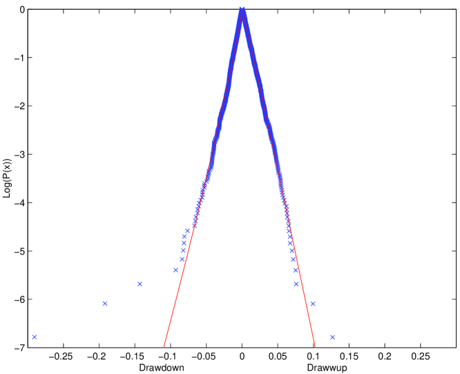
Figure 5: Same as figure 1 for the All Ordinaries index (Sydney stock exchange, Australia).

Figure 7: Same as figure 1 for the Hang Seng index (Hong Kong stock exchange).

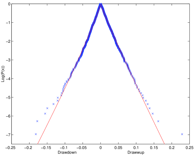
Figure 8: Same as figure 1 for the Nikkei 225 index (Tokyo stock exchange, Japan).

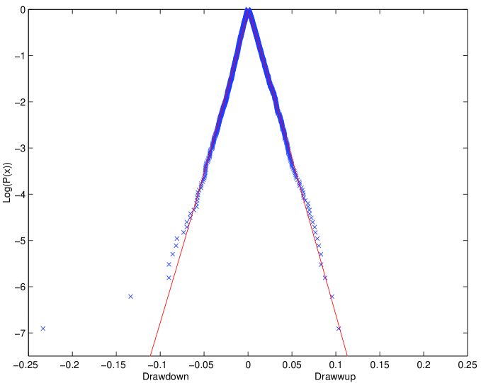
Figure 9: Same as figure 1 for the FTSE 100 composite index (London stock exchange, U.K.).

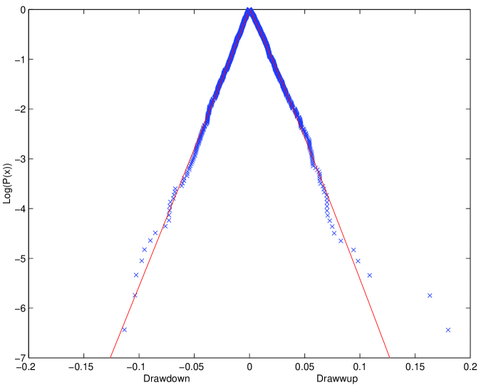
Figure 10: Same as figure 1 for the CAC40 index (Paris stock exchange, France).

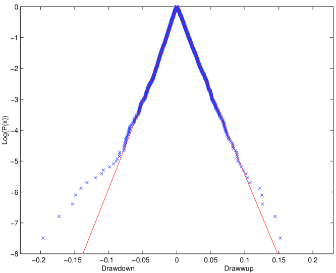
Figure 11: Same as figure 1 for the DAX index (Frankfurt stock exchange, Germany).

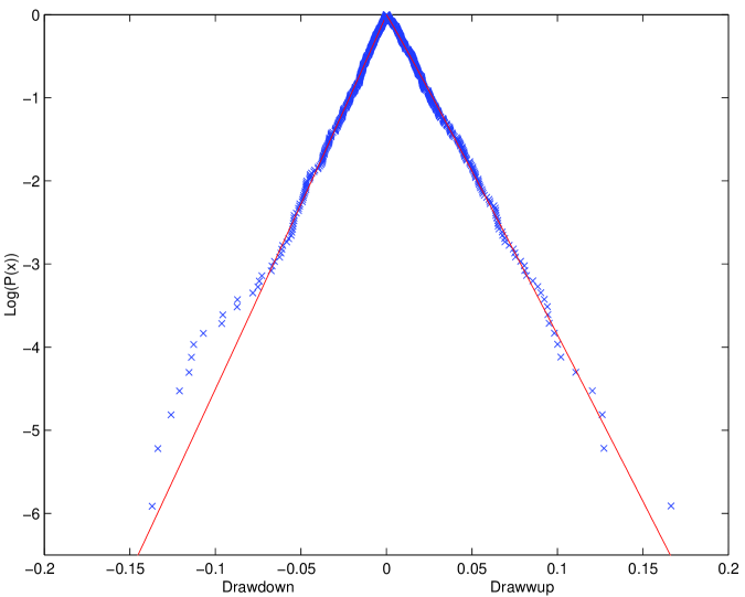
Figure 12: Same as figure 1 for the MIBTel index (Milan stock exchange, Italy).

Figure 14: Same as figure 1 for the US$/Yen exchange rate i.e., US $ expressed in Japanese Yen).

Figure 17: Difference (error plot) between the cumulative distribution of drawdowns and the best fit with the stretched exponential model (4) for the DJIS, the S&P500, the Nasdaq composite index, the German mark in US $ and Gold.

Figure 18: Difference (error plot) between the complementary cumulative distribution of drawups and the best fit with the stretched exponential model (4) for the DJIS, the S&P500, the Nasdaq composite index, the German mark in US $ and Gold.

Figure 19: Cumulative distribution of drawdowns and complementary distributions of drawups for the “time series neighborhoods” defined in section 3.4 obtained by adding noise to the DJIA time series. The four curves corresponds respectively to $A=0$ (no added noise), $A=0.5$ (added noise of standard deviation $\sigma/6$), $A=1$ (added noise of of standard deviation $\sigma/3$) and $A=2$ (added noise of of standard deviation $2\sigma/3$), where $\sigma$ is the standard deviation of the returns.

Figure 20: Same as figure 19 for the S&P500 index.

Figure 21: Same as figure 19 for the Nasdaq composite index.

Figure 22: Cumulative distribution of drawdowns and complementary cumulative distribution of drawups for $29$ companies, which include the $20$ largest USA companies in terms of capitalisation according to Forbes at the beginning of the year 2000, and in addition Coca Cola (Forbes number 25), Qualcomm (number 30), Appl. Materials (number 35), Procter & Gamble (number 38) JDS Uniphase (number 39), General Motors (number 43), Am. Home Prod. (number 46), Medtronic (number 50) and Ford (number 64). This figure plots each distribution $N_{c}$ normalized by its corresponding factor $A$ as a function of the variable $y\equiv|x|/\chi)^{z}$, where $\chi$ and $z$ are specific to each distribution and obtained from the fit to the stretched exponential model (4).

FIGURE 23

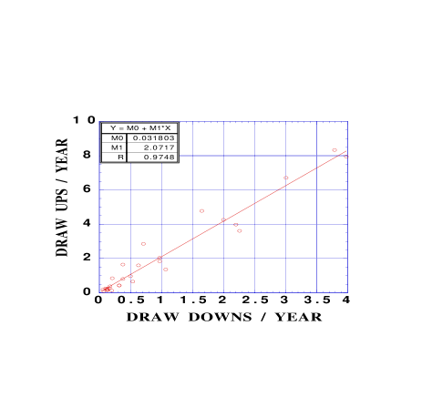
Figure 23: Number of drawups of amplitude larger than $15\%$ as a function of the number of drawdowns of amplitude larger than $15\%$ for all the companies analyzed here and shown respectively in tables 5 and 4. The linear regression is shown as the straight line and the parameters are given in the table within the figure. The correlation coefficient is $0.62$.

rank	starting time	index value	duration (days)	loss
1	$87.786$	$2508.16$	4	$-30.7\%$
2	$14.579$	$76.7$	2	$-28.8\%$
3	$29.818$	$301.22$	3	$-23.6\%$
4	$33.549$	$108.67$	4	$-18.6\%$
5	$32.249$	$77.15$	8	$-18.5\%$
6	$29.852$	$238.19$	4	$-16.6\%$
7	$29.835$	$273.51$	2	$-16.6\%$
8	$32.630$	$67.5$	1	$-14.8\%$
9	$31.93$	$90.14$	7	$-14.3$
10	$32.694$	$76.54$	3	$-13.9\%$
11	$74.719$	$674.05$	11	$-13.3\%$
12	$30.444$	$239.69$	4	$-12.4\%$
13	$31.735$	$109.86$	5	$-12.9$
14	$98.649$	$8602.65$	4	$-12.4\%$

Table 1: Characteristics of the 14 largest drawdowns of the Dow Jones Industrial Average in this century. The starting dates are given in decimal years.

Index	$A$ (fixed)	$B$	$\chi$ (%)	$z$	Time period of data
DJ	$6486$	$37.7$	$1.33\pm 0.02$	$0.84\pm 0.01$	[1900.0:2000.5]
S&P	$3363$	$54.8$	$1.17\pm 0.02$	$0.90\pm 0.01$	[1940.9:2000.5]
Nasdaq	$1495$	$31.9$	$1.32\pm 0.04$	$0.80\pm 0.02$	[1971.1:2000.5]
TSE 300 Composite	$833$	$52.7$	$1.05\pm 0.04$	$0.87\pm 0.02$	[1971.1:2000.5]
All Ordinaries	$881$	$49.7$	$1.24\pm 0.05$	$0.89\pm 0.02$	[1984.6:2000.5]
Straits Times	$683$	$25.7$	$1.56\pm 0.08$	$0.78\pm 0.02$	[1988.0:2000.5]
Hang Seng	$1171$	$23.7$	$2.11\pm 0.08$	$0.82\pm 0.02$	[1980.1:2000.5]
Nikkei 225	$1063$	$35.0$	$1.84\pm 0.07$	$0.89\pm 0.02$	[1973.0:2000.5]
FTSE 100	$997$	$58.9$	$1.31\pm 0.05$	$0.94\pm 0.02$	[1984.3:2000.5]
CAC 40	$623$	$54.4$	$1.77\pm 0.08$	$0.99\pm 0.03$	[1990.0:2000.5]
DAX	$1784$	$52.3$	$1.55\pm 0.04$	$0.95\pm 0.02$	[1970.0:2000.5]
MIBTel	$370$	$43.3$	$2.03\pm 0.11$	$0.98\pm 0.03$	[1993.0:1999.1]
Currencies	$A$ (fixed)	$B$	$\chi$	$z$	Time period of data
German Mark	$1826$	$77.7$	$0.84\pm 0.02$	$0.91\pm 0.02$	[1971.0:1999.4]
Japaneese Yen	$1706$	$54.9$	$1.17\pm 0.03$	$0.90\pm 0.02$	[1972.0:1999.4]
Swiss Franc	$1813$	$67.8$	$0.97\pm 0.03$	$0.91\pm 0.02$	[1971.0:1999.4]
Gold	$1681$	$38.6$	$1.29\pm 0.04$	$0.84\pm 0.02$	[1975.0:1999.8]

Table 2: Parameter values obtained by fitting equation (4) to the cumulative distribution $N_{c}$ of drawdowns. In order to stabilize the fit, it has been performed as $\log(N_{c})=\log(A)-B|x|^{z}$, where $A$ is the total number of drawdowns and hence fixed equivalent to a normalisation of the corresponding probability distribution. The characteristic scale $\chi$ is defined by $\chi=1/B^{1/z}$. DJ is the Dow Jones Industrial Average, S&P is the Standard and Poor 500 Index, Nasdaq is the Nasdaq Composite, TSE 300 Composite is the index of the stock exchange of Toronto, Canada, All Ordinaries is that of Sydney stock exchange, Australia, Straits Times is that of Singapore stock exchange, Hang Seng is that of Hong Kong stock exchange, Nikkei 225 is that of Tokyo stock exchange, Japan, FTSE 100 is that of London stock exchange, U.K., CAC 40 is that of Paris stock exchange, France, Dax is that of Frankfurt stock exchange, Germany and MIBTel is that of Milan stock exchange. The error bars reported for $\chi$ and $z$ are obtained from the formulas (5) and (6).

Index	$A$ (fixed)	$B$	$\chi(\%)$	$z$	Time period of data
DJ I	$6508$	$63.8$	$1.50\pm 0.02$	$0.99\pm 0.01$	[1900.0:2000.5]
DJ II	$\ln(A)\approx 8.09$	$16.5$	$0.73\pm 0.02$	$0.57\pm 0.005$	[1900.0:2000.5]
S&P	$3394$	$79.7$	$1.43\pm 0.04$	$1.03\pm 0.02$	[1940.9:2000.5]
Nasdaq	$1495$	$38.9$	$1.71\pm 0.05$	$0.90\pm 0.02$	[1971.1:2000.5]
TSE 300 Composite	$844$	$50.7$	$1.34\pm 0.05$	$0.91\pm 0.02$	[1984.3:2000.5]
All Ordinaries	$885$	$74.9$	$1.58\pm 0.05$	$1.04\pm 0.03$	[1984.6:2000.5]
Straits Times	$687$	$22.6$	$1.74\pm 0.09$	$0.77\pm 0.02$	[1988.0:2000.5]
Hang Seng	$1175$	$31.3$	$2.59\pm 0.08$	$0.96\pm 0.02$	[1980.1:2000.5]
Nikkei 225	$1066$	$37.2$	$2.05\pm 0.07$	$0.93\pm 0.02$	[1973.0:2000.5]
FTSE 100	$999$	$71.1$	$1.59\pm 0.05$	$1.03\pm 0.03$	[1984.3:2000.5]
CAC 40	$627$	$64.0$	$2.05\pm 0.08$	$1.07\pm 0.03$	[1990.0:2000.5]
DAX	$1785$	$52.1$	$1.77\pm 0.05$	$0.98\pm 0.02$	[1970.0:2000.5]
MIBTel	$369$	$41.6$	$2.57\pm 0.12$	$1.03\pm 0.04$	[1993.0:1999.1]
Currencies	$A$ (fixed)	$B$	$\chi(\%)$	$z$	Time period of data
German Mark	$1797$	$63.0$	$0.81\pm 0.02$	$0.86\pm 0.02$	[1971.0:1999.39]
Japaneese Yen	$1710$	$74.6$	$0.79\pm 0.02$	$0.89\pm 0.02$	[1972.0:1999.39]
Swiss Franc	$1815$	$61.5$	$0.93\pm 0.03$	$0.88\pm 0.02$	[1971.0:1999.39]
Gold	$1676$	$36.7$	$1.37\pm 0.04$	$0.84\pm 0.02$	[1975.0:1999.8]

Table 3: Parameter values obtained by fitting equation (4) to the cumulative distribution $N_{c}$ drawups. In order to stabilize the fit, it has been performed as $\log(N_{c})=\log(A)-B|x|^{z}$, where $A$ is the total number of drawups and hence fixed equivalent to a normalisation of the corresponding probability distribution. DJ is the Dow Jones Industrial Average, S&P is the Standard and Poor 500 Index, Nasdaq is the Nasdaq Composite, TSE 300 Composite is the index of the stock exchange of Toronto, Canada, All Ordinaries is that of Sydney stock exchange, Australia, Straits Times is that of Singapore stock exchange, Hang Seng is that of Hong Kong stock exchange, Nikkei 225 is that of Tokyo stock exchange, Japan, FTSE 100 is that of London stock exchange, U.K., CAC 40 is that of Paris stock exchange, France, Dax is that of Frankfurt stock exchange, Germany and MIBTel is that of Milan stock exchange.

Company	$A$ (fixed)	$B$	$\chi(\%)$	$z$	Time period	DD/year $>15\%$
MicroSoft	$884$	$36.1$	$3.18\pm 0.11$	$1.04\pm 0.03$	[1986.2:2000.5]	$0.63$
Cisco	$620$	$41.4$	$4.04\pm 0.15$	$1.16\pm 0.04$	[1990.2:2000.5]	$0.97$
General Elec.	$1866$	$51.6$	$2.09\pm 0.05$	$1.02\pm 0.02$	[1970.0:2000.5]	$0.13$
Intel	$846$	$33.0$	$3.69\pm 0.13$	$1.06\pm 0.03$	[1986.5:2000.5]	$1.07$
Exxon-Mobil	$1875$	$70.5$	$1.94\pm 0.04$	$1.08\pm 0.02$	[1970.0:2000.5]	$0.07$
Oracle	$757$	$28.7$	$4.73\pm 0.16$	$1.10\pm 0.03$	[1988.2:2000.5]	$2.20$
Lucent	$764$	$40.9$	$3.86\pm 0.13$	$1.14\pm 0.03$	[1996.3:2000.5]	$0.71$
Wall Mart	$1643$	$32.8$	$2.84\pm 0.08$	$0.98\pm 0.02$	[1972.7:2000.5]	$0.50$
IBM	$2404$	$44.2$	$2.09\pm 0.05$	$0.98\pm 0.02$	[1962.0:2000.5]	$0.13$
AT&T	$1918$	$46.6$	$1.91\pm 0.05$	$0.97\pm 0.02$	[1970.0:2000.5]	$0.13$
Citigroup	$1444$	$36.6$	$2.54\pm 0.07$	$0.98\pm 0.02$	[1977.0:2000.5]	$0.21$
Sun Microsystem	$832$	$30.1$	$4.53\pm 0.15$	$1.10\pm 0.03$	[1987.2:2000.5]	$2.26$
Texas Instruments	$1114$	$30.4$	$3.63\pm 0.11$	$1.03\pm 0.02$	[1982.0:2000.5]	$0.97$
HP	$1454$	$39.5$	$3.12\pm 0.08$	$1.06\pm 0.02$	[1977.0:2000.5]	$0.38$
SBC Communications	$980$	$48.1$	$2.08\pm 0.07$	$1.00\pm 0.02$	[1984.6:2000.5]	$0.06$
Merck	$1825$	$48.9$	$2.29\pm 0.05$	$1.03\pm 0.02$	[1970.0:2000.5]	$0.13$
EMC	$721$	$30.6$	$4.59\pm 0.16$	$1.11\pm 0.03$	[1989.0:2000.5]	$1.65$
Pfizer	$1144$	$47.9$	$2.60\pm 0.08$	$1.06\pm 0.02$	[1982.0:2000.5]	$0.32$
AOL	$504$	$18.1$	$5.37\pm 0.25$	$0.99\pm 0.03$	[1992.2:2000.5]	$3.98$
MCI WorldCom	$654$	$41.0$	$3.52\pm 0.13$	$1.11\pm 0.03$	[1990.2:2000.5]	$0.38$
Coca Cola	$1839$	$42.6$	$2.17\pm 0.05$	$0.98\pm 0.02$	[1970.0:2000.5]	$0.16$
Oualcomm	$537$	$26.7$	$5.61\pm 0.22$	$1.14\pm 0.04$	[1992.0:2000.5]	$3.01$
Appl. Materials	$963$	$30.0$	$5.06\pm 0.15$	$1.14\pm 0.03$	[1985.0:2000.5]	$2.00$
Procter&Gamble	$1857$	$42.8$	$1.92\pm 0.05$	$0.95\pm 0.02$	[1970.0:2000.5]	$0.20$
JDS Uniphase	$402$	$21.0$	$5.66\pm 0.28$	$1.06\pm 0.04$	[1993.9:2000.5]	$3.79$
General Motors	$1871$	$62.3$	$2.50\pm 0.05$	$1.12\pm 0.02$	[1970.0:2000.5]	$0.10$
Am. Home Prod.	$1100$	$40.3$	$2.21\pm 0.07$	$0.97\pm 0.02$	[1982.0:2000.5]	$0.32$
Medtronic	$1072$	$32.2$	$3.55\pm 0.11$	$1.04\pm 0.02$	[1982.0:2000.5]	$0.54$
Ford	$1481$	$49.6$	$2.60\pm 0.07$	$1.07\pm 0.02$	[1977.0:2000.5]	$0.17$

Table 4: The parameter values obtained by fitting equation (4) to the cumulative distribution $N_{c}$ of drawdowns. In order to stabilise the fit, it has been performed as $\log(N_{c})=\log(A)-B|x|^{z}$, where $A$ is the total number of drawdowns and hence fixed equivalent to a normalisation of the corresponding probability distribution. The companies are the top 20 in terms of market value, number 25, number 30, number 35, number 39 (no data for number 40 could be obtained), number 46 (no data for number 45 could be obtained) and number 50. Three more companies have been added in order to get longer time series as well as representatives for the automobil sector. These are Procter & Gamble (number 38), General Motors (number 43) and Ford (number 64). The ranking is Forbes of year 2000.

Company	$A$ (fixed)	$B$	$\chi(\%)$	$z$	Time period	DU/year $>15\%$
MicroSoft	$880$	$25.3$	$4.08\pm 0.14$	$1.01\pm 0.03$	[1986.2:2000.5]	$1.60$
Cisco	$617$	$32.0$	$4.84\pm 0.20$	$1.22\pm 0.04$	[1990.2:2000.5]	$2.04$
General Electric	$1877$	$43.9$	$2.45\pm 0.06$	$1.02\pm 0.02$	[1970.0:2000.5]	$0.20$
Intel	$850$	$38.9$	$4.85\pm 0.14$	$1.21\pm 0.03$	[1986.5:2000.5]	$1.36$
Exxon-Mobil	$1895$	$57.8$	$2.18\pm 0.05$	$1.06\pm 0.02$	[1970.0:2000.5]	$0.10$
Oracle	$761$	$25.1$	$5.77\pm 0.19$	$1.13\pm 0.03$	[1988.2:2000.5]	$3.98$
Lucent	$260$	$27.4$	$5.20\pm 0.30$	$1.12\pm 0.05$	[1996.3:2000.5]	$2.86$
Wall Mart	$1664$	$27.6$	$3.50\pm 0.09$	$0.99\pm 0.02$	[1972.7:2000.5]	$0.97$
IBM	$2400$	$39.0$	$2.29\pm 0.05$	$0.97\pm 0.02$	[1962.0:2000.5]	$0.26$
AT&T	$1854$	$32.1$	$1.94\pm 0.05$	$0.88\pm 0.02$	[1970.0:2000.5]	$0.16$
Citigroup	$1423$	$25.6$	$2.95\pm 0.09$	$0.92\pm 0.02$	[1977.0:2000.5]	$0.85$
Sun Microsystem	$827$	$26.4$	$5.66\pm 0.18$	$1.14\pm 0.03$	[1987.2:2000.5]	$3.61$
Texas Instruments	$1112$	$26.6$	$4.40\pm 0.13$	$1.05\pm 0.02$	[1982.0:2000.5]	$1.84$
HP	$1447$	$35.5$	$3.67\pm 0.09$	$1.08\pm 0.02$	[1977.0:2000.5]	$0.81$
SBC Communications	$972$	$38.1$	$2.44\pm 0.08$	$0.98\pm 0.02$	[1984.6:2000.5]	$0.19$
Merck	$1816$	$41.2$	$2.61\pm 0.06$	$1.02\pm 0.02$	[1970.0:2000.5]	$0.16$
EMC	$702$	$19.4$	$6.26\pm 0.23$	$1.07\pm 0.03$	[1989.0:2000.5]	$4.78$
Pfizer	$1137$	$38.1$	$3.12\pm 0.09$	$1.05\pm 0.02$	[1982.0:2000.5]	$0.43$
AOL	$493$	$18.1$	$5.35\pm 0.26$	$0.99\pm 0.03$	[1992.2:2000.5]	$7.95$
MCI WorldCom	$653$	$25.5$	$4.44\pm 0.18$	$1.04\pm 0.03$	[1990.2:2000.5]	$1.65$
Coca Cola	$1841$	$34.9$	$2.57\pm 0.06$	$0.97\pm 0.02$	[1970.0:2000.5]	$0.26$
Oualcomm	$537$	$18.1$	$6.68\pm 0.28$	$1.07\pm 0.04$	[1992.0:2000.5]	$6.71$
Appl. Materials	$961$	$30.0$	$5.06\pm 0.15$	$1.14\pm 0.03$	[1985.0:2000.5]	$4.26$
Procter&Gamble	$1857$	$47.3$	$2.37\pm 0.06$	$1.03\pm 0.02$	[1970.0:2000.5]	$0.13$
JDS Uniphase	$419$	$14.2$	$7.61\pm 0.38$	$1.03\pm 0.04$	[1993.9:2000.5]	$8.33$
General Motors	$1856$	$39.6$	$2.62\pm 0.06$	$1.01\pm 0.02$	[1970.0:2000.5]	$0.26$
Am. Home Prod.	$1092$	$31.5$	$2.55\pm 0.09$	$0.94\pm 0.02$	[1982.0:2000.5]	$0.43$
Medtronic	$1098$	$32.2$	$2.49\pm 0.08$	$1.04\pm 0.02$	[1982.0:2000.5]	$0.65$
Ford	$1481$	$35.9$	$2.89\pm 0.08$	$1.01\pm 0.02$	[1977.0:2000.5]	$0.38$

Table 5: The parameter values obtained by fitting equation (4) to the cumulative distribution $N_{c}$ of drawups. In order to stabilise the fit, it has been performed as $\log(N_{c})=\log(A)-B|x|^{z}$, where $A$ is the total number of drawups and hence fixed equivalent to a normalisation of the corresponding probability distribution. The characteristic scale $\chi$ is defined by $\chi=1/B^{1/z}$. The companies are the top 20 in terms of market value, number 25, number 30, number 35, number 39 (no data for number 40 could be obtained), number 46 (no data for number 45 could be obtained) and number 50. Three more companies have been added in order to get longer time series as well as representatives for the automobil sector. These are Procter & Gamble (number 38), General Motors (number 43) and Ford (number 64). The ranking is Forbes of year 2000. The error bars reported for $\chi$ and $z$ are obtained from the formulas (5) and (6).

Index	Threshold	Real data	Surrogate data	Confidence level
Dow Jones I. A.	$-18\%$	$5$	$0,0,491,387,110,12$	$\approx 99\%$
S&P500	$-10\%$	$7$	$0,0,183,337,283,130,48,15,4$	$\approx 99.5\%$
Nasdaq Comp.	$-14\%$	$5$	$478,398,117,7$	$\approx 99\%$
TSE 300 Comp .	$-10\%$	$4$	$0,642,300,54,4$	$\approx 99.5\%$
All Ordinaries	$-14\%$	$3$	$0,941,55,3,1$	$\approx 99.9\%$
Strait Times	$-29\%$	$1$	$1000,0$	$\approx 100\%$
Hang Seng	$-23\%$	$5$	$0,0,791,193,13,3$	$\approx 99.5\%$
Nikkei 225	$-14\%$	$4$	$0,1,384,354,173,66,18,3,1$	$\approx 75\%$
FTSE 100	$-23\%$	$1$	$996,4$	$\approx 99.5\%$
CAC 40	No	visible	outliers	$\approx 0\%$
DAX	$-13\%$	$6$	$0,452,391,122,32,2,1$	$\approx 99.9\%$
MIBTel	No	visible	outliers	$\approx 0\%$
Currencies	Threshold	Real data	Surrogate data	Confidence level
DM/US$	$-8\%$	$3$	$620,305,69,5,1$	$\approx 99.9\%$
YEN/US$	$-12\%$	$3$	$863,137$	$\approx 100\%$
CHF/US$	$-9\%$	$3$	$706,245,45,4$	$\approx 99.5\%$
Gold	$-17\%$	$4$	$799,182,19$	$\approx 100\%$

Table 6: For each of the indices and currencies named in the first column, a threshold given by the second column has been chosen by identifying identifying the point of breakdown from the stretched exponential, i.e., the crossover point from bulk to outliers in the distribution (the first point after the crossover point is then the smallest outlier and the threshold is the integer value of that drawdown). The third column gives the number of drawdowns above the threshold in the true data. The fourth column gives the number of surrogate data sets with $0,1,2,3,...$ drawdowns larger than the threshold. The last column quantifies the corresponding confidence level.

Company	Threshold	True data	Surrogate data	Confidence level
Microsoft (MSFT)	$-30\%$	$2$	$0,777,205,17,1$	$\approx 78\%$
Cisco	$-34\%$	$1$	$817,178$	$\approx 82\%$
General Electric (GE)	$-29\%$	$1$	$969,31$	$\approx 97\%$
Intel (INTC)	$-33\%$	$2$	$739,239,22$	$\approx 98\%$
Exxon-Mobil (XOM)	$-18\%$	$2$	$1,929,67,3$	$\approx 93\%$
Lucent (LU)	$-26\%$	$2$	$2,844,140,14$	$\approx 85\%$
Wall Mart (WMT)	$-22\%$	$6$	$236,341,281,107,28,7$	$\approx 100\%$
IBM	$-30\%$	$1$	$0,991,9$	$\approx 0\%$
AT&T (T)	$-24\%$	$4$	$0,0,0,952,47,1$	$\approx 95\%$
Citigroup (C)	$-21\%$	$5$	$0,1,577,337,69,16$	$\approx 98.5\%$
Sun Microsystem (SUNW)	$-40\%$	$1$	$701,251,44,4$	$\approx 70\%$
Texas Instruments (TXN)	$-36\%$	$2$	$0,505,476,19$	$\approx 50\%$
Hewlett Packard (HWP)	$-29\%$	$1$	$506,407,79,8$	$\approx 50\%$
SBC Communications (SBC)	$-20\%$	$1$	$929,68,3$	$\approx 93\%$
Merck (MRK)	$-20\%$	$2$	$775,206,16$	$\approx 98\%$
EMC	$-39\%$	$1$	$0,891,105,4$	$\approx 0\%$
Pfizer (PFE)	$-16\%$	$6$	$0,127,290,262,209,77,27,7,1$	$\approx 96.5\%$
MCI WorldCom (WCOM)	$-22\%$	$3$	$31,150,257,251,178,88,31,9,5$	$\approx 18\%$
Coca Cola (KO)	$-29\%$	$2$	$0,998,2$	$\approx 100\%$
Qualcomm (QCOM)	$-39\%$	$1$	$623,310,61,6$	$\approx 70\%$
Appl. Materials (AMAT)	$-36\%$	$2$	$475,390,114,19,2$	$\approx 87\%$
Procter&Gamble (PG)	$-37\%$	$2$	$0,0,1000$	$\approx 0\%$
General Motors (GM)	$-30\%$	$1$	$776,224$	$\approx 78\%$
Medtronic (MDT)	$-29\%$	$1$	$928,69,3$	$\approx 93\%$
Ford (F)	$-27\%$	$1$	$785,211,4$	$\approx 78\%$

Table 7: For each of the companies named in the first column, a threshold given by the second column has been chosen by identifying the point of breakdown from the stretched exponential, i.e., the crossover point from bulk to outliers in the distribution (the first point after the crossover point is then the smallest outlier and the threshold is the integer value of that drawdown). The third column gives the number of drawdowns above the threshold in the true data. The fourth column gives the number of surrogate data sets with $0,1,2,3,...$ drawdowns larger than the threshold. The last column quantifies the corresponding confidence level.