The response function of a sphere in a viscoelastic two–fluid medium

Abstract

In order to address basic questions of importance to microrheology, we study the dynamics of a rigid sphere embedded in a model viscoelastic medium consisting of an elastic network permeated by a viscous fluid. We calculate the complete response of a single bead in this medium to an external force and compare the result to the commonly–accepted, generalized Stokes–Einstein relation (GSER). We find that our response function is well approximated by the GSER only within a particular frequency range determined by the material parameters of both the bead and the network. We then discuss the relevance of this result to recent experiments. Finally we discuss the approximations made in our solution of the response function by comparing our results to the exact solution for the response function of a bead in a viscous (Newtonian) fluid.

]

I Introduction

Microrheology[1] has become an important experimental probe of the mechanical properties of soft materials such as actin or other bio-polymers[2, 3]. It is a class of experimental techniques that measure the response of probe particles to external forces. It is generally accepted that the response functions measured in microrheology experiments determine the same material properties as do traditional rheology experiments. In other words, one expects that it is possible to express the response function measured in microrheology in terms of the complex shear modulus, $G(\omega)$. This connection between the measured response function and $G(\omega)$ allows one to obtain rheological data for materials that cannot be produced in large quantity or to study the local rheological properties of rheologically inhomogeneous materials. An important example of a system which satisfies both of the above criteria is the living cell. Microrheology, therefore, promises to open an new window on cellular biology[4, 5].

There are currently two classes of techniques used to measure probe–particle responses. In the active technique, probe particles are subjected to an external force (e.g. magnetic[5, 6, 7] or laser tweezers[8]), and their displacements are measured with the aid of microscopes and imaging technology. In the passive technique, thermally fluctuating positions of particles are measured either via direct observation[10] or via light scattering[1, 3, 9] and the response function is then determined with the aid of the fluctuation–dissipation theorem. In either case we emphasize that there is an essential role to be played by theory to establish the connection between the measured response function and the underlying material properties of the medium being investigated. It is generally assumed[1, 3] that this connection is provided by the generalized Stokes–Einstein relation (GSER) in which the position ${\bf r}(\omega)$ of the probe particle (of radius $a$) as a function of frequency is given by

$${\bf r}(\omega)=\frac{1}{6\pi aG(\omega)}\,{\bf F}(\omega),$$ (1)

where ${\bf F}(\omega)$ is the applied force on the particle and $G(\omega)$ is the complex shear modulus. This result is the natural generalization of the Stokes mobility of the a rigid, spherical particle in a viscous fluid where the complex shear modulus reduces to $G(\omega)=-i\omega\eta$. One can certainly measure the mobility of such a spherical probe particle of known radius in a Newtonian fluid by observing its Brownian fluctuations (passive mode) or by a sedimentation experiment (active mode) and thereby determine the viscosity of the medium[11]. The generalization of this result embodied by the GSER [Eq. (1)] suggests that the analogous experiments performed in an arbitrary viscoelastic material will allow one to similarly obtain $G(\omega)$ for that material by the application of Eq. (1).

In this paper we examine the validity of the GSER through detailed calculations of the response of a rigid, spherical probe particle in a model viscoelastic medium. In particular, we study a two–fluid model[12] of a generic viscoelastic medium in which a viscoelastic network is viscously coupled to a permeating fluid. This model, which we study in a continuum limit, may be taken to represent a gel or an uncrosslinked polymer solution studied at frequencies larger than its plateau frequency.

There are two basic reasons to question the validity of the GSER: First, the mode structure of a multi-component medium is more complex than that of a simple fluid. A probe particle moving at frequency $\omega$ will excite modes other than simple shear modes, and its response to external forces will, in general, depend on all of these modes in a way not simply described by $G(\omega)$. Second, at frequencies accessible to microrheology experiments, which are much greater than those accessible to traditional rheology experiments, effects of the inertia of both the particle and the medium[13], which are not included either in the simple Stokes–Einstein relation or in the GSER, may be important. We will investigate both of these effects.

The fundamental results of this work have already been presented elsewhere[14]; here we elucidate the details of our approximate calculational scheme as well as provide a further discussion of the results. The remainder of this paper is organized as follows: In section II we discuss the basic two–fluid model in some detail, describing the hydrodynamic modes of the system. In section III we describe the approximate calculation of the response of a rigid, spherical particle embedded in such a medium. Using a comparison of the results of our technique to the well-known result for the drag on an oscillating sphere in a viscous fluid[15], we discuss the range of validity of our approximation. In section IV we determine the requisite conditions for the response function to be approximated by the GSER and detail the cross–over to non–GSER like behavior as a function of frequency. Finally we conclude in section V with a discussion of the limits of the validity of the GSER in which we apply our results to the experiments of Schnurr et al.[3]. In addition we compare the importance of inertial effects in traditional rheology to those in microrheology. The full calculation of the inertial effects upon a traditional, parallel–plate, rheological measurement applied to our two-fluid model is presented in the appendix.

II The Two–Fluid Medium

Our model viscoelastic medium consists of a viscoelastic network characterized by a displacement variable ${\bf u}$ that is viscously coupled via a friction coefficient $\Gamma$ to an incompressible, Newtonian fluid characterized by a velocity field ${\bf v}$. (See Fig. 1.) The viscoelastic network with mesh size $\xi$ is macroscopically isotropic and homogeneous. At length scales larger than $\xi$, it is characterized by an isotropic continuum elasticity with shear and bulk Lamè coefficients $\mu$ and $\lambda$, which may in general be complex functions of frequency $\omega$. Because of the viscous coupling of the elastic network to the fluid, there is a drag force density acting on the network due to its motion through the fluid, in addition to the force densities resulting from the local, network strain field.

The linearized equation of motion for the displacement field in the presence of an externally imposed force density ${\bf f}^{\rm u}$ acting directly on the network is

$$\rho\ddot{{\bf u}}-\mu\nabla^{2}{\bf u}-\left(\lambda+\mu\right)\nabla\left({\bf\nabla}\cdot{\bf u}\right)=-\Gamma\left(\dot{{\bf u}}-{\bf v}\right)+{\bf f}^{\rm u},$$ (2)

where $\rho$ is the mass density of the network. The frictional force density in the above equation is proportional to the local relative velocity of the network and the background fluid as is required by Galilean invariance. We may estimate the viscous coupling constant $\Gamma$ as follows: If a strand of the network of length equal to the characteristic mesh size $\xi$ moves relative to background fluid at a velocity ${\bf v}$, the drag force it experiences is approximately $\eta\xi{\bf v}$ where $\eta$ is the fluid viscosity. The drag force density on the network, given by $\Gamma{\bf v}$ in Eq. (2) above, is then $\eta\xi{\bf v}/\xi^{3}\sim\eta{\bf v}/\xi^{2}$. We then determine that $\Gamma\sim\eta/\xi^{2}$.

The fluid velocity field ${\bf v}$ obeys the linearized, incompressible Navier-Stokes equation with viscosity $\eta$. Including the drag of the network upon the fluid, we find

$$\rho_{\rm F}\dot{{\bf v}}-\eta\nabla^{2}{\bf v}+{\bf\nabla}P = \Gamma\left(\dot{{\bf u}}-{\bf v}\right)+{\bf f}^{\rm v}$$ (3)

$${\bf\nabla}\cdot\left[\left(1-\phi\right){\bf v}+\phi\dot{{\bf u}}\right] = 0,$$ (4)

where $\rho_{\rm F}$ is the mass density of the fluid, $\phi$ is the volume fraction of the elastic network, and $P$ is the pressure. ${\bf f}^{\rm v}$, in analogy to ${\bf f}^{\rm u}$, is an externally imposed force density acting on the fluid. We note that Eq. (4) demands the incompressibility of the total solution rather than that of the solvent (background fluid) alone. However, as we are primarily interested in discussing microrheological experiments on stiff bio-polymers such as actin, which form entangled solutions at extremely low volume fractions[16], we may assume that $\phi\ll 1$. In this limit Eq. (4) becomes the standard condition of the incompressibility of the background fluid, ${\bf\nabla}\cdot{\bf v}\simeq 0$. Similarly, because of the sparseness of the net we may assume that $\rho(=\phi\rho_{\rm net})\ll\rho_{\rm F}(=(1-\phi)\rho_{\rm fluid})$ where $\rho_{\rm net}$ and $\rho_{\rm fluid}$ are, respectively, the densities of the pure network and solvent. Because of this inequality we will later be able to simplify our results by making the reasonable approximation that $\rho\simeq 0$.

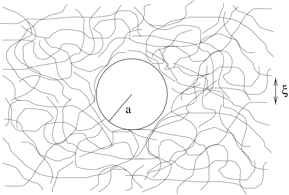
FIG. 1.: Microscopic model of the two–fluid medium. The viscoelastic network is represented by the lines in the figure. The network has a characteristic mesh size given by $\xi$. The probe particle is a sphere of radius $a$ shown in the center of the figure. The background viscous fluid (not shown) permeates the network.

Lastly we comment on the validity of the linearization of the Navier-Stokes equation in Eq. (3). In order for our linearization to be valid, the force density associated with the convective term $\rho{\bf v}\cdot{\bf\nabla}{\bf v}$ omitted from the linearized Navier–Stokes equation coupled to ${\bf u}$ [Eq. (3)] must be small compared to the other force densities in the system. To get a sense of when this term is unimportant, we investigated excitations at frequency $\omega$ in the large $\omega\Gamma$ limit in which the effective linearized velocity equation becomes

$${\rho}_{\rm F}\dot{{\bf v}}-\frac{G(\omega)}{-i\omega}\nabla^{2}{\bf v}=0,$$ (5)

where $G(\omega)=\mu-i\omega\eta$. Thus the convective term can be neglected provided ${\bf v}\cdot{\bf\nabla}{\bf v}\ll 1/(-i\omega)[-\omega^{2}+G(\omega)/{\rho}_{\rm F}]{\bf v}$. Considering the harmonic motion of the particle with frequency $\omega$ and amplitude $\ell$, we find that there are two cases to study. First, at low frequencies the second term on the RHS of the above equation dominates over the first, and the linearization of the Navier-Stokes equation requires that $\omega^{2}a\ell\rho/G(\omega)\ll 1$, which is just the condition that the Reynolds number be small. At higher frequencies, however, the first or inertial term on the RHS of the above equation dominates over the second, and the linearization now must be based on the inequality, $\ell/a\ll 1$[15]. Thus, the analysis presented in this paper can be extended to high frequencies where the inertial terms dominate the response function and the particle Reynolds number is high, provided the amplitude of the probe particle’s oscillation is small compared to its own radius. Similar conclusions follow when $\omega\Gamma$ is not large. The ability to model high–frequency dynamics is important in the study of the response function since microrheology allows the experimenter, in principle, to probe response functions at very high frequencies. Current experiments, however, have not yet explored the mechanical response of beads at high enough frequencies to leave the low–Reynolds–number regime.

We now discuss the hydrodynamic modes of the two–fluid medium. An equilibrium crystal in a one–component fluid background (e.g. a colloidal solid) has nine hydrodynamic modes[19, 18] (modes with frequencies vanishing with wavenumber) arising from three broken translational symmetries and the conservation of two masses, energy, and momentum. There are, one heat diffusion, one relative mass diffusion, one vacancy diffusion, two longitudinal sound, and four transverse sound modes. In our model, network crosslinks are rigidly fixed so there is no vacancy diffusion. Our system is incompressible so there are no longitudinal sound modes. In addition, we ignore heat diffusion. We, therefore, expect our model two–fluid system to have five hydrodynamic modes: one relative mass diffusion mode and four transverse sound modes. Our fundamental dynamical equations [Eqs. (2)– (4)] contain three ${\bf u}$ equations with two time derivatives and two independent ${\bf v}$ equations with one time derivative, have a total of eight modes. We therefore expect to find three non-hydrodynamic modes in addition to the five hydrodynamic modes.

We now determine the modes of the two-fluid model by Fourier transforming Eqs. (2)–(4) with $\phi$ and the external forces ${\bf f}^{\rm u},{\bf f}^{\rm v}$ set to zero. After eliminating the pressure $P$ using the incompressibility of the fluid we find

$$\left[\Delta^{\rm T}({\bf k},\omega){\bf P}^{\rm T}_{\alpha\beta}+\Delta^{\rm L}({\bf k},\omega){\bf P}^{\rm L}_{\alpha\beta}\right]u_{\beta}-\Gamma v_{\alpha} = 0$$ (6)

$$i\omega\Gamma{\bf P}^{\rm T}_{\alpha\beta}u_{\beta}+\Pi({\bf k},\omega){\bf P}^{\rm T}_{\alpha\beta}v_{\beta} = 0$$ (7)

$${\bf P}^{\rm L}_{\alpha\beta}v_{\beta} = 0$$ (8)

where we have defined $\Delta^{\rm T}({\bf k},\omega)=-\omega^{2}\rho+\mu k^{2}-i\omega\Gamma$, $\Delta^{\rm L}({\bf k},\omega)=-\omega^{2}\rho+(2\mu+\lambda)k^{2}-i\omega\Gamma$, and $\Pi({\bf k},\omega)=-i\omega\rho_{\rm F}+\eta k^{2}+\Gamma$. We have also introduced the standard transverse (${\bf P}^{\rm T}({\bf k})=\delta_{\alpha\beta}-\hat{k}_{\alpha}\hat{k}_{\beta}$) and longitudinal (${\bf P}^{\rm L}_{\alpha\beta}({\bf k})=\hat{k}_{\alpha}\hat{k}_{\beta}$) projection operators. The condition for nontrivial solutions for ${\bf u}$ and ${\bf v}$ gives the following result:

$$\Delta^{\rm L}({\bf k},\omega)\left[i\omega\Gamma^{2}+\Delta^{\rm L}({\bf k},\omega)\Pi({\bf k},\omega)\right]^{2}=0.$$ (9)

The first factor on the left hand side of Eq. (9) is quadratic in $\omega$ while the second factor, which is cubic in $\omega$, is squared so that the total expression is an eighth order polynomial in $\omega$. Its roots, which correspond to the modes of the system, are clearly divided into two sets. The first set, which are roots of the first factor on the LHS of Eq. (9), consists of two longitudinal modes. The second set, coming from the roots of the second factor in Eq. (9), represent the remaining six transverse modes. These transverse modes come in three identical pairs corresponding to the two possible polarization states of the transverse waves. We first consider the transverse modes in more detail.

Ignoring the polarization–state degeneracy for the moment, two of the three transverse modes are a pair of propagating shear waves in the medium. For small $k$, the dispersion relation is given by

$$\omega({\bf k})=\pm\sqrt{\frac{\mu}{\rho+\rho_{\rm F}}}k-\frac{i}{2}\left[\frac{\mu{\rho}_{\rm F}^{2}}{\Gamma\left(\rho+{\rho}_{\rm F}\right)^{2}}+\frac{\eta}{\rho+\rho_{\rm F}}\right]k^{2}.$$ (10)

Counting polarization states, these shear modes constitute four of the five hydrodynamic modes of the system. The phase velocity is similar to that of the transverse sound modes in the elastic medium when decoupled from the background fluid. The shear wave speed of the two–fluid model is identical to that of a one–component elastic solid with mass density replaced by the total combined network – fluid mass density $\rho+\rho_{\rm F}$. The effect of the fluid coupling can be seen in the damping rate of this mode. In the weak coupling limit, where $\Gamma$ is small, the dominant contribution to the damping rate comes from the first term in the brackets which arises from the relative motion of the elastic network against the background fluid. The strong coupling limit, on the other hand, derives its damping from viscous dissipation (the second term in brackets) in the fluid which, in this limit, is sheared as it moves with the network. It should be noted that the $\Gamma\longrightarrow 0$, decoupled limit is not easily apparent in the above result. The long wave length approximation has been used in the above derivation which corresponds to taking $k\ll\sqrt{\Gamma/\eta}\sim 1/\xi$, where the last expression of the right hand side was produced using our estimate, $\Gamma\sim\eta/\xi^{2}$.

The third transverse mode has a finite decay rate at zero wavevector and corresponds to a relative motion of the network and fluid that comprises our two–component medium. To lowest order in wavevector its decay rate is given by

$$\omega({\bf k})=-i\Gamma\left(\frac{\rho_{\rm F}+\rho}{\rho_{\rm F}\rho}\right)$$ (11)

where we have dropped ${\cal O}(k^{2})$ corrections to the damping rate.

To examine the longitudinal modes of the medium it is convenient to allow the fluid to have a finite compressibility $\chi^{-1}={\rho}_{\rm F}\partial P/\partial\rho_{\rm F}$ at first and then to take the incompressible limit later. We, therefore, introduce a variable fluid density via $\rho_{\rm F}\longrightarrow\rho_{\rm F}+\delta\rho$, that obeys the equation of motion: $\dot{\delta\rho}=-{\rho}_{\rm F}{\bf\nabla}\cdot{\bf v}$. Projecting out only the longitudinal degrees of freedom of the system, we have to lowest order in wavevector a pair of propagating longitudinal sound modes with dispersion relations of the form:

$$\omega_{\rm sound}({\bf k})=\pm\sqrt{\frac{(2\mu+\lambda)+\chi{\rho}_{\rm F}}{\rho+{\rho}_{\rm F}}}k-id(\chi)k^{2},$$ (12)

where $d(\chi)k^{2}$ is the decay rate of the sound modes, and two over–damped modes with decay rates given by

$$\omega_{\rm long}({\bf k}) = -i\frac{(2\mu+\lambda){\rho}_{\rm F}\chi}{\Gamma\left(2\mu+\lambda+{\rho}_{\rm F}\chi\right)}k^{2},$$ (13)

$$\omega({\bf k}) = -i\frac{\Gamma\left(\rho+{\rho}_{\rm F}\right)}{\rho{\rho}_{\rm F}}.$$ (14)

We note the mode with a finite decay rate at $k=0$ [Eq. (14)] has an identical dispersion relation to the gapped transverse mode, Eq. (11). We, therefore, identify it as the longitudinal counterpart to the transverse modes in which there is relative motion between the network and the fluid. In the incompressible limit ($\chi\longrightarrow\infty$), the longitudinal sound velocity becomes infinite as expected. The decay rate diverges as well, $d(\chi)\longrightarrow\infty$, thus these two modes (Eq. 12) in which the network and fluid experience compressions and rarifactions do not concern us in the incompressible limit. What will be more interesting with regard to the calculation of the response of the bead is the fifth hydrodynamic mode (Eq. (13)) whose decay rate remains finite in the incompressible limit. In that limit we find that the decay rate takes the form

$$\lim_{\chi\longrightarrow\infty}\omega_{\rm long}({\bf k})=-i\frac{2\mu+\lambda}{\Gamma}k^{2}.$$ (15)

This mode is the relative mass diffusion mode of the system. The network density (described by $\delta\rho/\rho=-{\bf\nabla}\cdot{\bf u}$) changes and relaxes diffusively while that of the background fluid remains fixed. The existence of a slowly decaying longitudinal mode not present in an incompressible viscous fluid has consequences for the validity of the GSER in our two–fluid model.

III Calculating the Response Function

To calculate the response of the probe particle to an applied force, we will need to introduce the rigid probe particle into the two–fluid medium described in the previous section. The complete solution of the problem requires that one solve Eqs. (2)–(4) with time derivatives replaced by $-i\omega$, ${\bf f}^{\rm u}$, ${\bf f}^{\rm v}$ set equal to zero, and the enforcement of the correct boundary conditions at the surface of the probe sphere, i.e.,

$${\bf u}\left(\left|{\bf x}\right|=a,\omega\right)={\bf v}\left(\left|{\bf x}\right|=a,\omega\right)/-i\omega={\bf r}(\omega),$$ (16)

where ${\bf r}(\omega)$ is the frequency–dependent position of the center of the probe sphere. In addition we would need to apply the boundary condition that both ${\bf u}$ and ${\bf v}$ go to zero far from the sphere. After calculating the displacement and velocity fields, ${\bf u}({\bf x},\omega)$ and ${\bf v}({\bf x},\omega)$, that solve this boundary value problem, we would then calculate, the force ${\bf F}_{\rm b}$ exerted on the sphere by the medium by integration of the appropriate components of the stress tensor over the surface of the probe sphere. Newton’s second law applied to the probe sphere (of mass $M$) under the influence of the externally applied force ${\bf F}(\omega)$,

$$-\omega^{2}M{\bf r}(\omega)-{\bf F}_{\rm b}(\omega)={\bf F}(\omega),$$ (17)

leads to a determination of the response function $\alpha(\omega)$, where $\alpha$ is defined by

$${\bf r}(\omega)=\alpha(\omega){\bf F}(\omega).$$ (18)

The calculation outlined above is possible for the case of a simple viscous medium but becomes more difficult for the two–fluid medium we study. We will, therefore, apply a less rigorous procedure. To justify this approximation we verify in Appendix A that our method does, in fact, reproduce the correct frequency–dependent response function over some finite frequency range in the simpler problem of a sphere in a Newtonian fluid. Fortunately, the interesting features of microrheological measures can still be explored in the frequency range still available to our investigation.

Here we briefly outline our approximate calculation: As a first step in this procedure, we restore the applied force densities ${\bf f}^{\rm u}$ and ${\bf f}^{\rm v}$ in the equations of motion. We then calculate the the displacement field ${\bf u}$ and the fluid velocity field ${\bf v}$ everywhere in the medium as a function of the, as yet undetermined values of the two applied force densities, ${\bf f}^{\rm u}$ and ${\bf f}^{\rm v}$. These force densities will be used to represent the forces applied to the medium by the probe sphere. We, therefore, localize these forces at the sphere by setting

$${\bf f}^{\rm u,v}({\bf k},\omega)={\bf F}^{\rm u,v}(\omega)\Theta\left(k_{\rm max}-\left|{\bf k}\right|\right),$$ (19)

where $\Theta(x)$ is the unit step function and $k_{\rm max}=\pi/2a$ is the large wavevector cutoff. One role of the bead is to cut off the spectrum of allowed fluctuations of the medium at the length scale of the probe particle radius. It it then clear that the wavevector cutoff is proportional to the inverse particle radius; the numerical coefficient is chosen to produce the correct low–frequency Stokes mobility of the spherical particle in a Newtonian fluid as verified in Appendix A. We note that this abrupt cutoff in Fourier space cannot be strictly valid as we really want a sharp cutoff in the real space, applied–force profile. However, we will show that this simple scheme is sufficient to reproduce standard hydrodynamic results concerning the frequency–dependent response of an oscillating sphere in a viscous fluid which we believe justifies our confidence in our more general application of the approach.

Following the procedure outlined above, we now have a solution for the motion of the bead in terms of two, as yet unknown, forces ${\bf F}^{\rm u},{\bf F}^{\rm v}$ due to the bead acting on the elastic network and viscous fluid respectively. We determine a relation between these two forces by requiring that the boundary condition Eq. (16) at the sphere sphere be satisfied. The total force that the bead exerts on the two-fluid medium is therefore given by: $-{\bf F}_{\rm b}=-{\bf F}^{\rm u}-{\bf F}^{\rm v}$. We have now calculated the displacement of the sphere in terms of ${\bf F}_{\rm b}$. By inverting this relation and using it in Eq. (17) can calculate the response function.

To implement this procedure we first determine ${\bf u}$ and ${\bf v}$ in terms of the applied forces ${\bf f}^{\rm u,v}$. We find

$${\cal G}_{ij}^{-1}\cdot\left(\begin{array}[]{c}u_{j}\\ v_{j}\end{array}\right)=\left(\begin{array}[]{c}f^{{\rm u}}_{j}\\ {\bf P}^{\rm T}_{jk}f^{{\rm v}}_{k}\end{array}\right).$$ (20)

The $6\times 6$ matrix ${\cal G}^{-1}$, described in detail in appendix B, can be decomposed into a $2\times 2$ matrix of $3\times 3$ blocks. In Eq. (20) the vectorial indices (shown) run over all three spatial directions while the indices labeling the $2\times 2$ blocks (suppressed) run over the space spanned by the displacement field (${\bf u}$) and the fluid velocity field (${\bf v}$). To determine ${\bf u}$ and ${\bf v}$ in terms of the applied forces on the medium, ${\bf f}^{\rm u}$, and ${\bf f}^{\rm v}$ we simply need to invert ${\cal G}^{-1}$. This inversion is easy owing to the fact that the four $3\times 3$ blocks of the matrix, displayed in Appendix B, all mutually commute.

We now integrate this result over all wavevectors, ${\bf k}$, to determine the fluctuating position (${\bf r}(\omega)$) and velocity (${\bf w}(\omega)$) of the point at the origin of the (unstressed) material. Because the problem is isotropic we find that the vectorial part of each $2\times 2$ block is particularly simple (see Appendix B):

$$G^{\rm(n,m)}(\omega)\delta_{ij}=\int_{\left|{\bf k}\right|<k_{\rm max}}{\cal G}^{({\rm n,m})}_{ij}({\bf k},\omega)\frac{d^{3}k}{(2\pi)^{3}}.$$ (21)

The limits on the wavevector integral come from the cutoff imposed by the rigidity of the sphere, Eq. (19). We have a pair of equations specifying the position and velocity of the point at the origin of the two–fluid medium (the position of the sphere) in terms of the force on the elastic network and the transverse part of the force on the fluid,

$$r_{i}(\omega) = G^{{\rm(u,u)}}(\omega)F^{{\rm u}}_{i}(\omega)+G^{{\rm(u,v)}}(\omega)F^{{\rm v}}_{i}(\omega)$$ (22)

$$w_{i}(\omega) = G^{{\rm(v,u)}}(\omega)F^{{\rm u}}_{i}(\omega)+G^{{\rm(v,v)}}(\omega)F^{{\rm v}}_{i}(\omega).$$ (23)

The boundary condition, Eq. (16), becomes $w_{i}(\omega)=-i\omega r_{i}(\omega)$. Imposing this condition on Eqs.(22), (23) fixes the ratio of ${\bf F}^{{\rm u}}(\omega)$ to ${\bf F}^{{\rm v}}(\omega)$. Using this ratio we write the displacement of the sphere, ${\bf r}(\omega)$, in terms of the total force that the sphere exerts on the medium, $-{\bf F}_{\rm b}(\omega)$:

$${\bf r}(\omega)=-\gamma(\omega){\bf F}_{\rm b}(\omega),$$ (24)

where the function $\gamma(\omega)$ is given by

$$\gamma(\omega)=\frac{1}{1-X(\omega)}\left[G^{{\rm(u,u)}}(\omega)-G^{{\rm(u,v)}}(\omega)X(\omega)\right],$$ (25)

where the function $X(\omega)$ can be written in terms of the $G$’s as well:

$$X(\omega)=\frac{i\omega G^{{\rm(u,u)}}(\omega)+G^{{\rm(v,u)}}(\omega)}{i\omega G^{{\rm(u,v)}}(\omega)+G^{{\rm(v,v)}}(\omega)}.$$ (26)

Using Eq. (24) in Eq. (17) to eliminate ${\bf F}_{\rm b}$, we find the position response of the bead to an applied force as defined in Eq. (18).

$$\alpha^{-1}(\omega)=\gamma^{-1}(\omega)-\omega^{2}M.$$ (27)

In essence Eqs. (25),(26) and Eq. (27) completely determine our solution for the response function. In order to study the detailed form of the response function, however, we need to discuss the four $G^{\rm(n,m)},({\rm n,m}={\rm u,v})$ as functions of frequency. We begin this task in the next section by first discussing each of the four $G$’s in turn and then looking in detail at the response function, $\alpha(\omega)$ which is made up of these $G$’s.

IV The Response Function

We first look at the response of the elastic network to forces applied directly to that network, $G^{{\rm(u,u)}}(\omega)$. We introduce the following notation: the complex shear modulus of the two–fluid medium will be denoted by the usual $G(\omega)=\mu(\omega)-i\omega\eta$. It should be noted that whereas $\eta$ represents the viscosity of the background solvent – see our estimate of the drag force density coefficient $\Gamma$ – the elastic network may in general be viscoelastic. Its shear modulus will be given in general by a complex, frequency–dependent shear modulus, $\mu$. We find that $G^{{\rm(u,u)}}(\omega)$ takes the form:

$$G^{{\rm(u,u)}}(\omega)=\frac{1}{6\pi aG(\omega)}\left[1+\frac{G(\omega)}{4\mu+2\lambda}H\left(\frac{\omega}{\omega_{\rm B}}\right)+J(\omega)\right]$$ (28)

where the function $H(x)$ is specified by the integral:

$$H(x)=1-\int_{0}^{1}\frac{dz}{1+\frac{iz^{2}}{x}}.$$ (29)

This function is plotted in figure 2. The function $J(\omega)$ is given by

$$J(\omega)=\int_{0}^{1}dz\frac{\beta(\omega)+\Delta_{0}(z,\omega)z^{2}\left(1-\mu/G(\omega)\right)}{z^{2}\left(1+\mu\Delta_{0}(z,\omega)/G(\omega)\right)-\beta(\omega)}.$$ (30)

The frequency scale,

$$\omega_{\rm B}=\frac{\left(2\mu+\lambda\right)}{\Gamma}k_{\rm max}^{2},$$ (31)

has also been introduced in Eq. (28). In addition to defining these two functions, we have introduced a set of new, frequency–dependent parameters. The first of these is

$$\beta(\omega)=\frac{\omega^{2}{\rho}_{\rm F}}{k_{\rm max}^{2}G(\omega)}=\frac{4a^{2}\omega^{2}{\rho}_{\rm F}}{G(\omega)\pi^{2}},$$ (32)

which measures the importance of the fluid inertia in determining the dynamics of the medium as may be noted by checking that this parameter can be expressed as the ratio of the sphere radius to the inertial decay length in the two–fluid medium[20]. We have also introduced the parameter $\Delta_{0}(z,\omega)$ defined by

$$\Delta_{0}(z,\omega)=\frac{-i\omega{\rho}_{\rm F}+\eta k^{2}_{\rm max}z^{2}}{\Gamma}\approx-i\omega\xi^{2}/\nu+\left(zk_{\rm max}\xi\right)^{2},$$ (33)

which may be identified as the inverse viscous response function divided by the drag coefficient $\Gamma$. Using our estimate for the drag coefficient, we may determine the magnitude of $\Delta_{0}$ under the conditions of a typical microrheological experiment. The first term on the RHS of Eq. (33) measures the ratio of the observation frequency to the viscous dissipation rate at the length scale of the network mesh size $\xi$. We may estimate this latter time scale for typical experiments on actin[3] to be in the $10$MHz range, well above any other frequencies of interest. Thus $\omega\ll\nu/\xi^{2}$. Similarly the second term at the right of Eq. (33) is small assuming that the sphere is much larger than the mesh size, $a\gg\xi$. We may reasonably set $\Delta_{0}$ to zero while discussing our result. The expression Eq. (30) may then be greatly simplified by noting that $\Delta_{0}$ is vanishingly small under the typical conditions of a microrheological experiment. With this approximation we rewrite Eq. (30) as

$$J(\omega)\approx\beta(\omega)\int_{0}^{1}dz\frac{1}{z^{2}-\beta(\omega)}.$$ (34)

It is now clear from this simplified, approximate form that $J(\omega)$ contains corrections to the response function coming from the inertia of the two–fluid medium. In direct analogy with the long–time tails in a Newtonian fluid (see Appendix A), the lowest order in frequency inertial corrections coming from Eq. (34) are of the form $\sqrt{\beta(\omega)}$. In a purely viscous medium this produces the standard $\omega^{1/2}$ corrections. In the viscoelastic medium, which we now study, the frequency dependence of the corrections will depend on the detailed form of the complex shear modulus. We take up this point again in discussing the actin system in our conclusions.

Returning to the function $H$ introduced in Eq. (28) and defined by Eq. (29), we note that for large $x$, the function goes to zero as $H(x)\sim i/(3x)$. See figure 2. For observation frequencies much larger than the frequency scale $\omega_{\rm B}$, the term proportional to $H(\omega/\omega_{\rm B})$ goes to zero, while for frequencies much less than $\omega_{\rm B}$, this term makes a finite correction to the response function. The physical interpretation of the $H$ function is made clear by recognizing that the crossover frequency is simply the decay time of the network compression mode [whose dispersion relation is given in Eq. (15)] at the length scale of the bead. At frequencies much lower than $\omega_{\rm B}$, the effect of the network compression mode upon the dynamics of the bead is significant while at frequencies high compared to $\omega_{\rm B}$ the network is viscously locked to the incompressible fluid. Therefore, this longitudinal mode of the network plays no role in the high–frequency bead dynamics. The function $H(\omega/\omega_{\rm B})$ controls the cross-over from compressible network dynamics to incompressible network Finally we note that the zero–frequency response of the network to a localized force on the network takes the Stokes mobility form, which is a standard result in the mechanics of elastic media.

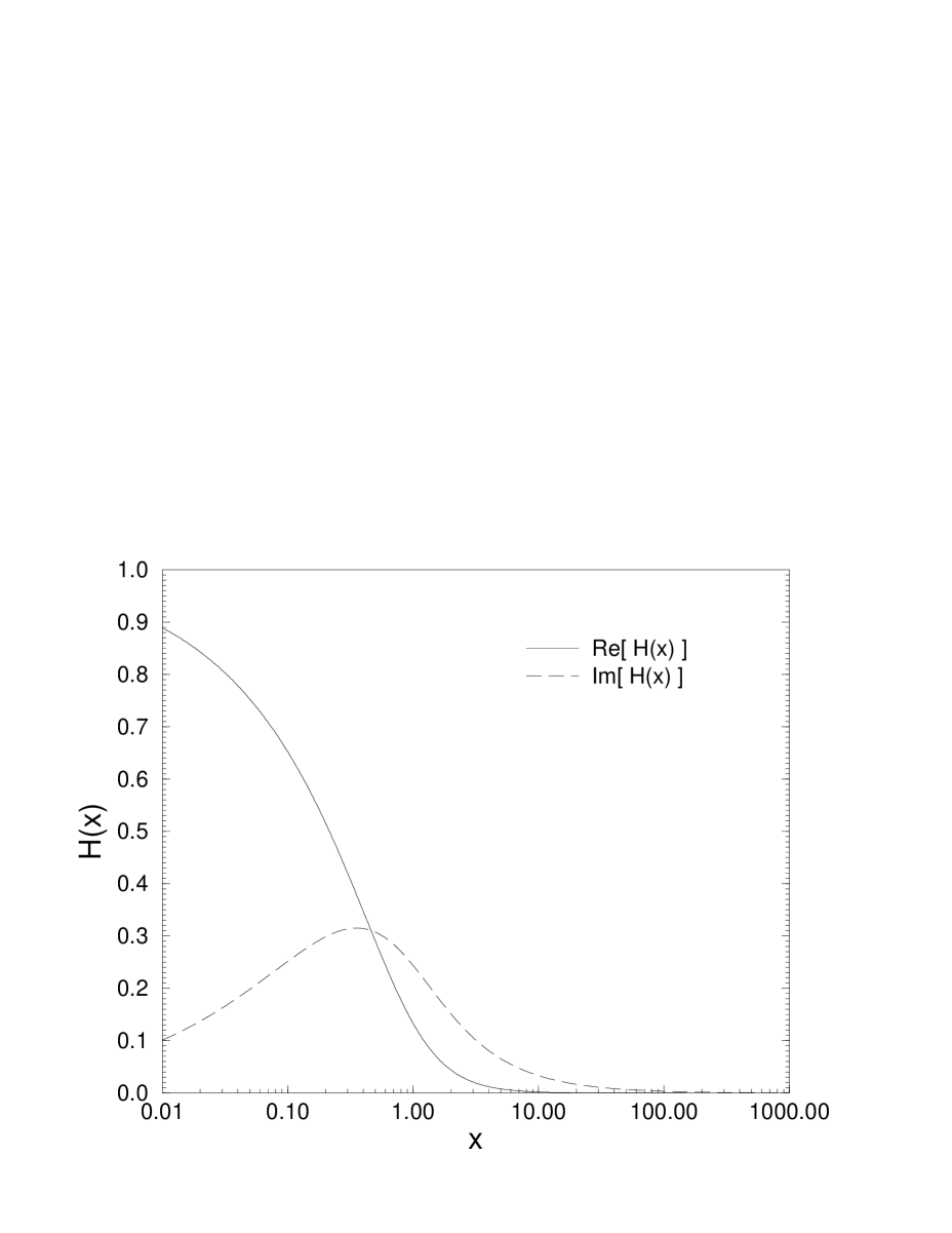
FIG. 2.: The real and imaginary parts of the cross over function $H(x)$, which determines the crossover from low–frequency ($\omega\ll\omega_{\rm B}$) behavior, in which the network compressibility plays a role in the dynamics of the bead, to the high–frequency ($\omega\gg\omega_{\rm B}$) incompressible dynamics. In the response function $x$ is the ratio of the observation frequency to the frequency scale $\omega_{\rm B}$.

Continuing our exploration of the response function, we consider the response of the network to a force on the fluid, $G^{{\rm(u,v)}}$. We find that this term has the form

$$G^{{\rm(u,v)}}(\omega)=\frac{1}{6\pi aG(\omega)}\int_{0}^{1}dz\frac{z^{2}}{z^{2}\left(1+\Delta_{0}(z,\omega)\frac{\mu}{G(\omega)}\right)-\beta(\omega)}.$$ (35)

Once again we may set $\Delta_{0}(z,\omega)=0$ making only a small error in the combined limits: $\omega\ll\nu/\xi^{2},k_{\rm max}\xi\ll 1$ so we may simplify the above expression to yield

$$G^{{\rm(u,v)}}(\omega)\simeq 1+J(\omega),$$ (36)

where $J(\omega)$ was defined in Eq. (30).

We are now in a position to see under what limiting conditions will the calculated response function reduce to the GSER. Examining $\alpha(\omega)$ at low enough frequencies so that we may ignore the bead inertia term ($-\omega^{2}M$) we find the response function to be

$$\alpha(\omega) \simeq \frac{1}{6\pi aG(\omega)}\left[1+J(\omega)+\right.$$ (38)

$$+\left.\frac{1}{1-X(\omega)}\frac{G(\omega)}{4\mu+2\lambda}H\left(\frac{\omega}{\omega_{\rm B}}\right)\right].$$

For bead dynamics at frequency $\omega$ small enough so that we may ignore the inertial corrections contained in $J(\omega)$, i.e. $\omega<\omega^{\star},\beta(\omega^{\star})=1$, we may set $J=0$. If, on the other hand, $\omega$ is much larger than $\omega_{\rm B}$ we may ignore corrections to the bead’s fluctuations coming from the thermal excitation of the network compression mode and thus set $H(\omega/\omega_{\rm B})=0$. Since we will be able to show that for typical values of the material parameters (in actin solutions for example[3]) $\omega_{\rm B}<\omega^{\star}$, there will exist a range of frequencies, $\omega_{\rm B}\longleftrightarrow\omega^{\star}$, for which the response function is well approximated by the GSER. In order to discuss deviations from the GSER, however, we need to study the form of $X(\omega)$.

We find that the function $X(\omega)$ is given by

$$X(\omega) = \frac{i\omega\eta}{\mu\left(k_{\rm max}\xi\right)^{2}}\times$$ (40)

$$\left[\int_{0}^{1}dz\frac{z^{4}}{z^{2}\left(1+\frac{\mu}{G(\omega)}\Delta_{0}(z,\omega)\right)-\beta(\omega)}\right]^{-1}\times$$

$$\times \left\{\int_{0}^{1}dz\frac{z^{2}\Delta_{0}(z,\omega)}{\left(1+\frac{\mu}{G(\omega)}\Delta_{0}(z,\omega)\right)z^{2}-\beta(\omega)}\right.$$ (41)

$$+ \left.\frac{G(\omega)}{2\lambda+4\mu}H\left(\frac{\omega}{\omega_{\rm B}}\right)\right\}$$ (42)

It is important to note that the prefactor multiplying $X(\omega)$ above contains $(k_{\rm max}\xi)^{-2}$ which we have argued is typically quite large. The large number is, however, multiplied by the ratio of the viscous stress in the background fluid to the stress in the viscoelastic network. For experimentally realizable frequencies this ratio is quite small. Thus $X(\omega)$ presents a small correction to the response function in a majority of interesting cases. We develop this point further in the discussion of these result presented in the next section.

V Summary

The response function of the rigid, spherical probe particle in the two–fluid medium has been calculated, see Eqs. (27), (38). Through a detailed study of the position response function of the probe particle embedded in a two–fluid, viscoelastic medium to an externally applied force, we have checked the validity of the GSER. Our results show that there exits a frequency range, $\omega_{\rm B}\longleftrightarrow\omega^{\star},\left|\beta(\omega^{\star})\right|=1$, over which the GSER is a good approximation to the full response function. We now consider recent experiments on actin solutions to determine the width of this regime, and if it is possible experimentally detect the deviations from GSER behavior.

In recent actin experiments[3], the shear modulus was found to be well approximated over a frequency range extending from about $10$Hz (above the plateau frequency) to the highest measured frequencies of a few KHz by:

$$G^{\prime}_{\rm exp}(\nu)\simeq G^{\prime\prime}_{\rm exp}(\nu)\simeq\left(\frac{\nu}{({\rm Hz})}\right)^{3/4}10\frac{{\rm dynes}}{{\rm cm}^{2}}.$$ (43)

The $\nu^{3/4}$ frequency dependence is in agreement with the theories of a number of groups[7, 21]. The shear modulus of the network dominates over the shear viscosity in the background fluid up to very high frequencies. This may be checked by comparing $\left|G^{\prime}_{\rm exp}(\omega)\right|\simeq\left|G^{\prime\prime}_{\rm exp}(\omega)\right|$ to the viscous shear stress modulus: $\omega\eta$, taking the viscosity to be that of water. Using Eq. (43) we can compare the relative magnitudes of the shear stress in the the viscoelastic network to that of the background fluid ($\omega\eta$). Clearly at large enough frequencies the fluid will carry the larger part of the stress in the material, while below some crossover frequency, the network shear modulus is the the dominant contributor to the mechanical properties of the two–fluid material. A simple calculation shows that this crossover frequency is approximately $6\times 10^{8}{\rm Hz}$, which is well above all experimentally accessible frequencies so that the network shear modulus is always the principle contributor to the two–fluid shear modulus. It is this dominance of the network contribution to the shear modulus in the material that allows us to ignore corrections coming from $X(\omega)$ in our solution of the response function in Eq. (38). We now check whether inertial effects are important in these measurements which ranged up to frequencies of a few kHz. There are two sources of inertial effects: those coming from the fluid inertial and those coming from the mass of the probe particle. We first look at the fluid inertia. Using our expression for $\beta(\nu)$ in Eq. (32) we find the cross–over frequency, $\nu^{\star},\beta(\nu^{\star})=1$ to be given by

$$\nu^{\star}=\left(1.6a^{2}\right)^{-4/5}{\rm Hz}$$ (44)

where $a$ is measured in centimeters. The experiment employed probe sphere sizes ranging from one to five microns yielding cross–over frequencies in the range of $1.7$MHz — $131$kHz, which, given that these experiments probe frequencies up to only a few kHz, suggests that the onset of inertial effects should be unobservable at present. It should be remembered, however, that the cross–over to the inertial regime is slow, being governed by $\sqrt{\beta(\omega)}$ so the effects of fluid inertia may be detectable at significantly lower frequencies. Nevertheless, we do not believe that the present experiments are probing the fluid inertial regime. There is a similar inertial effect due to the mass of the probe particle. To determine the frequency onset of the signature of the probe particle’s inertia, we may compare the particle inertial term $-\omega^{2}M$ to the dominant contribution to the response function at high frequency, the generalized Stokes mobility of sphere, $6\pi G(\omega)a$. This comparison gives roughly the same estimates as from the fluid inertia estimate above. The similarity of the two estimates is not surprising since the probe particle is of nearly the same density as the fluid.

We note from appendix C that the effect of inertia is not negliable in the traditional rheological measurements of soft materials[22]. We find that if the soft material is probed using a standard parallel–plate shear cell, inertial corrections to the response function, $G(\omega)=\mu-i\omega\eta$, enter at frequencies such that the oscillating plates excite shear waves in the medium whose decay length is shorter than the plate separation $L$. In the limit that the plate separation is much larger than the mesh size of the network (a necessary assumption for the application of our continuum theory) these inertial corrections may be expressed in terms of a plate separation independent scaling factor. In this limit, the experimentally determined response function $G_{\rm exp}(\omega)$ is related to the expected, low–frequency response function $G(\omega)=\mu-i\omega\eta$ by the relation

$$G_{\rm exp}(\omega)=G(\omega)y\coth(y)$$ (45)

where the dimensionless variable $y$ is defined in terms of the plate separation $L$, and the shear wave speed $c$ and damping rate $\Delta$ — see Eq. (10) and Eqs. (C22),(C23) in appendix C:

$$y=\left(i\frac{\omega}{c}-\frac{\omega^{2}}{c^{3}}\Delta\right)L.$$ (46)

In the low–frequency limit such that $\left|y\right|\ll 1$ it is clear that this expression reduces to the expected result: $G_{\rm exp}(\omega)\simeq G(\omega)$. For the type of parallel–plate experiment under discussion, a sample thickness of one millimeter implies that the inertial corrections can be neglected for frequencies below $10$kHz. This upper bound on frequencies imposed by the appearance of inertial corrections is of the same order of magnitude as the analogous bound determined for the microrheology response function[14].

We now turn to the determination of the low–frequency limit of the GSER relation. The lower bound of this frequency range is given by $\omega_{B}$. Using our expression for $\omega_{\rm B}$ given in Eq. (31) we find that the low–frequency cross–over to the network compression regime occurs at

$$\nu_{\rm B}\simeq\frac{2\mu+\lambda}{\eta}\frac{\pi}{8}\left(\frac{\xi}{a}\right)^{2}.$$ (47)

Given typical material parameters for entangled actin solutions, taking the elastic moduli to be on the order of the plateau modulus and taking the network mesh size to be on the order of a tenth of a micron we find that $\nu_{\rm B}\simeq 1$Hz. This is on the order of the plateau frequency and is certainly probed by experiment.

To summarize our work we note that the response function probed by a single particle, microrheological experiment contains information about all of the hydrodynamic modes of the system. In other words the fluctuations of the probe particle are in response to all the thermally excited modes of the system, whereas in a standard, macrorheological experiment, one explicitly determines the response of the system to an externally applied shear strain. If the medium admits hydrodynamic modes that are not simply shear waves, the microrheological response function can not be expressed entirely in terms of the material’s complex shear modulus as determined from standard rheology. On the other hand, if the hydrodynamic modes of the medium are simply shear waves then we expect that the simple correspondence between microrheological and standard rheological measurements, as expressed by the GSER will hold at low enough frequencies. At higher frequencies, both techniques will encounter the inertial effects. Microrheology, however, allows the exploration of the mechanical response of the medium at much higher frequencies than those probed by standard rheology, so the importance of the inertia of both the medium and the probe particle itself cannot be overlooked a priori.

For the model viscoelastic medium which we have studied there is an extra hydrodynamic mode (as compared to an incompressible, viscous fluid) which introduces of lower frequency bound on the validity of the GSER. This lower bound has some experimental significance for entangled actin solutions as this lower bound occurs near to the frequency of the rubber plateau in this material. The inertial effects, however, should not be relevant to current experiments that study the high frequency, single chain dynamics of the system.

We would like to thank J.C. Crocker for communicating unpublished results and many useful discussions. We would also like to thank R.D. Kamien, F.C. MacKintosh, D.C. Morse, and A.G. Yodh for helpful discussions. This work was supported in part by the NSF MRSEC Program under grant No. DMR96–32598.

A The response of a sphere in a Newtonian fluid

In this appendix we test our approximate solution method by calculating the response function of a sphere in a Newtonian fluid. This problem has a well–known solution[15] which lets us check the validity of our approximation scheme. As throughout this article, we assume that the spherical particle undergoes simple harmonic motion of an amplitude small compared to its size so that we may neglect the flow advection term in the Navier–Stokes equation even in the high Reynolds number limit. The problem we wish to solve is simply stated: What is the force acting the bead if it is observed to undergo simple harmonic motion of the form: ${\bf v}={\rm Re}\left[v_{0}\exp\left(-i\omega t\right)\right]$?

The motion of the spherical particle (of mass $M$) obeys Newton’s second law:

$$M\dot{{\bf v}}={\bf F}+{\bf F}_{\rm b}$$ (A1)

where ${\bf F}$ is the externally applied force on the bead and ${\bf F}_{\rm b}$ is the force due to the fluid acting on the bead. We will use our approximation scheme to calculate that force, ${\bf F}_{\rm b}$. First we solve for the velocity field of the fluid given that some force ${\bf F}_{\rm v}({\bf x},t)={\bf F}_{\rm v}({\bf x},\omega)\exp(-i\omega t)$ is applied to it using

$${\rho}_{\rm F}\dot{{\bf v}}=\eta\nabla^{2}{\bf v}-{\bf\nabla}P+{\bf F}_{\rm v}({\bf x},t).$$ (A2)

Additionally, we require the incompressibility of the fluid:

$${\bf\nabla}\cdot{\bf v}=0.$$ (A3)

We calculate the fluid velocity at the origin (the location of the bead) by integrating over all wavevectors, ${\bf k}$,

$$v_{\alpha}({\bf x}=0,\omega)=\int\frac{d^{3}k}{(2\pi)^{3}}\frac{{\bf P}^{\rm T}_{\alpha\beta}({\bf k}){\bf F}_{\rm v}({\bf k},\omega)}{-i\omega{\rho}_{\rm F}+\eta k^{2}}$$ (A4)

Noting the spherical symmetry of the bead, we demand that ${\bf F}_{\rm v}({\bf k},\omega)={\bf F}(\omega){\cal F}(k)$ is a function of the magnitude of $k$ alone, allowing us to perform the angular integrations above and leading to the following result for $\gamma_{\rm v}$ defined by

$${\bf v}({\bf x}=0,\omega)=\gamma_{\rm v}(\omega){\bf F}(\omega).$$ (A5)

We determine

$$\gamma_{\rm v}(\omega) = \frac{1}{6\pi\eta a}\left[\frac{2}{\pi}\int_{0}^{\infty}dz{\cal F}(z)\right.$$ (A6)

$$+ \left.\frac{2i}{\pi}\frac{\omega}{\omega_{\nu}}\int_{0}^{\infty}dz{\cal F}(z)\frac{1}{z^{2}-i\omega/\omega_{\nu}}\right]$$ (A7)

where $z=ka$, the frequency scale $\omega_{\nu}=\nu a^{-2}$ (where $\nu=\eta/{\rho}_{\rm F}$ is the kinematic viscosity) is the viscous dissipation rate at the length scale of the sphere, and the as yet unknown function ${\cal F}$ is determined by the $k$ dependence of ${\bf F}_{\rm v}(\left|{\bf k}\right|,\omega)$, or, in other words, how we localize the force of the bead upon the fluid at the surface of the bead. One clear choice is to localize the force on the interface of the fluid and the sphere: ${\bf F}_{\rm v}({\bf x})=\frac{F}{2\pi a}\delta\left(\left|x\right|^{2}-a^{2}\right)$ where $F$ total force exerted by the sphere on the fluid and we have suppressed the oscillatory time dependence. An even simpler choice, which we have made throughout the paper, is localize the force in wavevector space via: ${\bf F}_{\rm v}({\bf k})=\Theta\left(\frac{\pi}{2a}-\left|k\right|\right)$. The first choice leads to ${\cal F}(z)=\frac{\sin(z)}{z}$ while the second version yields ${\cal F}(z)=\frac{\pi}{2}\Theta(1-z)$. Hereafter we refer to the first version as the “shell localization” and the second version as the “volume localization”.

Using the shell localization we find that Eq. (A6) simplifies to the exact expression:

$$\gamma_{\rm v}^{-1}(\omega)=6\pi\eta a\exp\left[\left(1-i\right)\sqrt{\frac{\omega}{2\omega_{\nu}}}\,\right].$$ (A8)

We will be concerned only with the expansion of the above expression for $\omega\ll\omega_{\nu}$. Using the volume localization, on the other hand, we find that the exact result to all orders is more complicated but to order $\sqrt{\omega/\omega_{\nu}}$ we find an identical result to that above (Eq. (A8)),

$$\gamma_{\rm v}^{-1}(\omega)=6\pi\eta a\left[1+\left(1-i\right)\sqrt{\frac{\omega}{2\omega_{\nu}}}+{\cal O}\left(\frac{\omega}{\omega_{\nu}}\right)\right].$$ (A9)

Of course, to this order in frequency, we may ignore the inertial of the bead and from Eq. (A1) we note that $\gamma_{\rm v}^{-1}(\omega)$ is then identical to the inverse response function we sought. This result agrees with the standard solution of this problem arrived at through the complete solution of the boundary value problem[15] to the order in frequency shown above. At higher orders in frequency, starting with ${\cal O}(\omega/\omega_{\nu})$ where the bead’s inertia comes into play, deviations between our approximate calculation of the fluid’s inertia and the exact result appear. Our result over estimates the ${\cal O}(\omega/\omega_{\nu})$ contribution to the fluid inertial by a factor of about $5.5$. Based on this analysis we expect similar accuracy in the two–fluid calculations using the volume localization scheme that are presented in this paper. As is discussed in the conclusions, the inaccuracy of our results at high frequencies is not relevant to the current set microrheological measurements. These experiments have not yet probed the transition to the inertial regime, which should, in fact, be well described by our (correct) order ${\cal O}(\sqrt{\omega/\omega_{\nu}})$ fluid inertia terms.

B The ${\cal G}^{-1}$ Matrix

Here we write the matrix ${\cal G}^{-1}$ in its $2\times 2$ block form. We introduce the viscous response function in the fluid: $\Delta^{-1}({\bf k},\omega)=-i\omega{\rho}_{\rm F}+\eta k^{2}$, and elastic response of the network, with additional damping due to the coupling to the viscous fluid, decomposed into its transverse, $D^{-1}_{\rm T}({\bf k},\omega)=-\omega^{2}\rho+\mu k^{2}-i\omega\Gamma$, and longitudinal, $D^{-1}_{\rm L}({\bf k},\omega)=-\omega^{2}\rho+\left(2\mu+\lambda\right)k^{2}-i\omega\Gamma$, parts. In terms of these functions we may write ${\cal G}^{-1}$ as

$$\left(\begin{array}[]{ccc}D^{-1}_{\rm T}({\bf k},\omega){\bf P}^{\rm T}_{ij}+D^{-1}_{\rm L}({\bf k},\omega){\bf P}^{\rm L}_{ij}&-\Gamma\delta_{ij}\\ i\omega\Gamma{\bf P}^{\rm T}_{ij}&\Delta^{-1}({\bf k},\omega)\delta_{ij}+\Gamma{\bf P}^{\rm T}_{ij}\end{array}\right).$$ (B1)

All four $3\times 3$ blocks shown above are proportional to either the identity matrix or the transverse or longitudinal projectors. Since all three of these matrices are mutually commuting we see that the inversion of ${\cal G}^{-1}$ is quite simple.

After performing this matrix inversion we find that the four $2\times 2$ blocks are given by:

$${\cal G}^{(1,1)}_{ij} = \frac{\left(\Delta^{-1}({\bf k},\omega)+\Gamma\right){\bf P}^{\rm T}_{ij}({\bf k})}{D^{-1}_{\rm T}({\bf k},\omega)\left(\Delta^{-1}({\bf k},\omega)+\Gamma\right)+i\omega\Gamma^{2}}+$$ (B2)

$$+ \frac{{\bf P}^{\rm L}_{ij}({\bf k})}{-\omega^{2}\rho+(2\mu+\lambda)k^{2}}$$ (B3)

$${\cal G}^{(1,2)}_{ij} = \frac{\Gamma{\bf P}^{\rm T}_{ij}({\bf k})}{\left(\Delta^{-1}({\bf k},\omega)+\Gamma\right)D^{-1}_{\rm T}({\bf k},\omega)+i\omega\Gamma^{2}}$$ (B4)

$${\cal G}^{(2,1)}_{ij} = \frac{-i\omega\Gamma{\bf P}^{\rm T}_{ij}({\bf k})}{\left(\Delta^{-1}({\bf k},\omega)+\Gamma\right)D^{-1}_{\rm T}({\bf k},\omega)+i\omega\Gamma^{2}}$$ (B5)

$${\cal G}^{(2,2)}_{ij} = \frac{D^{-1}_{\rm T}({\bf k},\omega){\bf P}^{\rm T}_{ij}({\bf k})}{\left(\Delta^{-1}({\bf k},\omega)+\Gamma\right)D^{-1}_{\rm T}({\bf k},\omega)+i\omega\Gamma^{2}}$$ (B6)

In the first of the above equations we have found the response of the network to a force on the network. The second (and third) of the response functions shown above gives the response of the network (fluid) to a force on the fluid (network). The final response function is the response of the fluid to a force on the fluid. This interpretation becomes clear in the decoupled limit where $\Gamma\longrightarrow 0$. Here the fluid and the network do not interact so ${\cal G}^{(1,2)}={\cal G}^{(2,1)}=0$. The response of the network to forces on the network is given by

$$\lim_{\Gamma\longrightarrow 0}{\cal G}^{(1,1)}_{ij}=\frac{{\bf P}^{\rm T}_{ij}({\bf k})}{-\omega^{2}\rho+\mu k^{2}}+\frac{{\bf P}^{\rm L}_{ij}({\bf k})}{-\omega^{2}\rho+(2\mu+\lambda)k^{2}},$$ (B7)

showing the standard transverse (first term) and longitudinal (second term) response of an isotropic, elastic medium to an applied force. The response of the fluid to a force on a fluid is similarly in accord with basic hydrodynamics,

$$\lim_{\Gamma\longrightarrow 0}{\cal G}^{(2,2)}_{ij}=\frac{{\bf P}^{\rm T}{ij}({\bf k})}{-i\omega{\rho}_{\rm F}+\eta k^{2}}.$$ (B8)

C Standard rheology on the two–fliud medium

In this appendix we calculate the response function of the medium to an externally applied shear strain in order to predict the result of a traditional rheological measurement. We check this result in order to compare it with the response of the probe particle discussed in this article. We do not expect to see any evidence of the longitudinal network mass density mode since the system will be subjected to a pure shear strain by moving the boundaries of the material. Nevertheless we do expect to observe departures of the shear response from the simple value of $G(\omega)=\mu-i\omega\eta$ due to inertial terms. We will thus compare the effect of inertial in the standard rheological experiment to the microrheological experiment via this calculation.

We begin with the equations of motion defining the two–fluid medium, Eqs. (2) – (4). We now consider a slab of this composite material held between two, parallel, rigid plates normal to the $\hat{z}$ axis located at $z=0,L$. The slab is unbounded in the $xy$ plane. In order to calculate the complex shear response of the material we will move the top plate ($z=L$) harmonically, ${\bf u}(z=L)=\hat{x}U_{0}e^{-i\omega t}$ while holding the bottom plate fixed. Given these boundary conditions we calculate the required shear stress on the top plate, $\sigma(z=L)_{xz}$. The ratio of this shear stress to the imposed shear strain $U_{0}/L$ is the complex shear complex shear modulus at the frequency $\omega$.

By the translational invariance of the problem in the $xy$ plane we may restrict our search for the resulting network displacement and fluid velocity fields to those of the form:

$${\bf u} = F(z)e^{-i\omega t}\hat{x}$$ (C1)

$${\bf v} = G(z)e^{-i\omega t}\hat{x}.$$ (C2)

Using the incompressibility of the fluid we find that $P$, the hydrostatic pressure is an harmonic function. Since the pressures at both plates are equal, $P$ is constant. Using Eqs. (2),(3) we find two coupled, ordinary differential equations for $F$ and $G$:

$$\mu\partial_{z}^{2}F+\rho\omega^{2}F+i\omega\Gamma F+\Gamma G = 0$$ (C3)

$$\eta\partial_{z}^{2}G+i\omega{\rho}_{\rm F}G-\Gamma G-i\omega\Gamma F = 0$$ (C4)

Putting in $F=F_{i}e^{\lambda_{i}z},G=G_{i}e^{\lambda_{i}z}$, we find that nontrivial solutions of the above differential equations can only exist for values of the $\lambda$ that solve the characteristic equation,

$$\eta\mu\lambda^{4}+\lambda^{2}\left[-\mu\Gamma+i\omega\left({\rho}_{\rm F}\mu+\eta\Gamma\right)+\eta\rho\omega^{2}\right]+$$ (C5)

$$+\left[-\omega^{2}\left(\rho+{\rho}_{\rm F}\right)\Gamma+i\omega^{3}{\rho}_{\rm F}\rho\right] = 0.$$ (C6)

The above equation has four roots coming in two pairs of roots having the same absolue value, i.e. $\lambda_{1},\ldots,\lambda_{4}$ where $\lambda_{1}^{2}=\lambda_{2}^{2}$ and $\lambda_{3}^{2}=\lambda_{4}^{2}$. Corresponding to these four eigenvalues there are four eigenvectors of the form: $\left(F_{i},\gamma_{i}F_{i}\right)$. It should be noted that, since the eigenvector equation depends only upon the square of the eigenvalue, the coefficients $\gamma_{i}$, $i=1,\ldots,4$ have the following relations: $\gamma_{1}=\gamma_{2}$ and $\gamma_{3}=\gamma_{4}$. We now may write the general solution to Eqs. (C3), (C4) as a linear superposition of the four eigenvectors discussed above:

$$F(z) = \sum_{i=1}^{4}F_{i}e^{\lambda_{i}z}$$ (C7)

$$G(z) = \sum_{i=1}^{4}\gamma_{i}F_{i}e^{\lambda_{i}z}.$$ (C8)

We have four boundary conditions to determine the remaining four constants. At the bottom plate we require stick boundary conditions for the fluid and the network at that immobile plate:

$$G(0)=F(0)=0.$$ (C9)

We also impose stick boundary conditions at the harmonically oscillating, upper plate:

$$G(L) = -i\omega U_{0}$$ (C10)

$$F(l) = U_{0}.$$ (C11)

Using the above boundary conditions we determine the network displacement field to be

$$F(z) = \frac{U_{0}}{\lambda_{1}^{2}-\lambda_{3}^{2}}\left[\lambda_{1}^{2}\frac{\sinh(\lambda_{3}z)}{\sinh(\lambda_{3}L)}-\lambda_{3}^{2}\frac{\sinh(\lambda_{1}z)}{\sinh(\lambda_{1}L)}\right]+$$ (C13)

$$+\frac{U_{0}}{\lambda_{1}^{2}-\lambda_{3}^{2}}\frac{\rho\omega^{2}}{\mu}\left[\frac{\sinh(\lambda_{3}z)}{\sinh(\lambda_{3}L)}-\frac{\sinh(\lambda_{1}z)}{\sinh(\lambda_{1}L)}\right],$$

and the fluid velocity field to be

$$G(z) = \frac{-i\omega U_{0}}{\lambda_{1}^{2}-\lambda_{3}^{2}}\left[\lambda_{1}^{2}\frac{\sinh(\lambda_{3}z)}{\sinh(\lambda_{3}L)}-\lambda_{3}^{2}\frac{\sinh(\lambda_{1}z)}{\sinh(\lambda_{1}L)}\right]+$$ (C15)

$$+\frac{-i\omega U_{0}}{\lambda_{1}^{2}-\lambda_{3}^{2}}\frac{i\omega{\rho}_{\rm F}}{\eta}\left[\frac{\sinh(\lambda_{3}z)}{\sinh(\lambda_{3}L)}-\frac{\sinh(\lambda_{1}z)}{\sinh(\lambda_{1}L)}\right].$$

We may now calculate the complex shear modulus that would be measured by a standard rheology experiment performed on our two–fluid medium. We calculate the applied stress stress divided by the applied shear strain to get the response function, $G_{\rm exp}(\omega)$.

$$G_{\rm exp}(\omega)=\left(\mu\left.\frac{dF}{dz}\right|_{z=L}+\eta\left.\frac{dG}{dz}\right|_{z=L}\right)\frac{L}{U_{0}}.$$ (C16)

After some minor rearrangements we arrive at

$$G_{\rm exp}(\omega)=\left[\left(\mu-i\omega\eta\right)+\frac{\omega^{2}\left(\rho+{\rho}_{\rm F}\right)}{\lambda_{1}\lambda_{3}}\right]J(L).$$ (C17)

In the above equation, the term in the parentheses is the expected result for the response function. It is simply the sum of the complex shear response of the network and the viscous response of the permeating fluid. The second term in the brackets is clearly an inertial correction to this standard result. Both of these terms are multiplied by a system size dependent scaling factor, $J(L)$. This function when expressed in terms of the dimensionless variables, $x=L\lambda_{1}$, $y=L\lambda_{3}$, takes the form

$$J(L)=\frac{xy}{x^{2}-y^{2}}\left[x\coth(y)-y\coth(x)\right].$$ (C18)

We expect that approximation: $G_{\rm exp}\simeq\mu-i\omega\eta$ should hold at least as the limiting behavior of $G_{\rm exp}(\omega)$ at low frequencies. To check this we need to consider the frequency dependence of the two eigenvalues appearing above: $\lambda_{1}$ and $\lambda_{3}$.

In the limit of low frequency we find that these roots of the characteristic polynomial, Eq. (C6) take the form:

$$\lambda_{1}^{2} = \frac{\Gamma}{\eta}-i\omega\left(\frac{{\rho}_{\rm F}\mu+\eta\Gamma}{\mu\eta}\right)+\frac{\omega^{2}{\rho}_{\rm F}}{\mu}+{\cal O}(\omega^{3})$$ (C19)

$$\lambda_{3}^{2} = -\frac{\omega^{2}\left(\rho+{\rho}_{\rm F}\right)}{\mu}-i\omega^{3}\left(\frac{{\rho}_{\rm F}+\rho}{\mu}\right)^{2}\times$$ (C20)

$$\times \left[\frac{\mu{\rho}_{\rm F}^{2}}{\left(\rho+{\rho}_{\rm F}\right)^{2}\Gamma}+\frac{\eta}{\rho+{\rho}_{\rm F}}\right]+{\cal O}(\omega^{4}).$$ (C21)

We note that $\lambda_{1}$ at low frequency is the inverse of a microscopic length since $\Gamma/\eta\sim\xi^{-2}$. In a macroscopic shear experiment of the type we are currently considering, the plate separation is much larger than this microscopic length: $L\lambda_{1}\gg 1$. In Eq. (C18) we may take $x=L\lambda_{1}\gg 1$. If we now take the modulus of $y$ to be small, $\left|y\right|=L\left|\lambda_{3}\right|\ll 1$ we find that $J(L)$ does, in fact, reduce to unity. The second limit is valid for low frequencies. To satisfy this inequality, both the imaginary and real parts of $y$ must be small. We consider the physical implications of these two conditions independently.

It may be checked by comparing Eq. (C20) to Eq. (10) that to lowest order in frequency, $\Re(y)=\frac{\Delta\omega^{2}}{c^{2}}\left(\frac{L}{c}\right)$ where $c$ is the transverse shear wave speed and $\Delta$ is the tranverse shear wave damping rate as given in Eq. (10),

$$c = \sqrt{\frac{\mu}{\rho+{\rho}_{\rm F}}}$$ (C22)

$$\Delta = \frac{1}{2}\left[\frac{\mu{\rho}_{\rm F}^{2}}{\left(\rho+{\rho}_{\rm F}\right)^{2}\Gamma}+\frac{\eta}{\rho+{\rho}_{\rm F}}\right].$$ (C23)

The imaginary part of $y$, on the other hand, takes the form: $\Im(y)=-L\omega/c$. Requiring that the modulus of $y$ to be small (and thus requiring both the imaginary and real parts of $y$ to be small) is equivalent to demanding that the sample be subjected to a uniform (affine) shear deformation as we discuss below. The standard intrepretation of a macroscopic–shear rheological experiment supposes that the sample has been affinely deformed by the imposed shear. The validity of that assumption is essential if one is to determine the complex shear modulus from a macroscopic–shear rheological experiment where the applied stress and resultant strain are measured only at the sample boundaries.

First, the condition that $\Re(y)\ll 1$ implies that the damping rate of the shear waves multiplied by the shear wave travel time across the sample must be small. In other words the shear wave in the two–fluid composite medium should not be appreciably damped on the length scale of the sample thickness. If, on the other hand, the sample thickness is much larger than the shear penetration depth, $\delta$, only the small portion of the sample of thickness equal to that penetration depth is strained. The shear strain in the sample that results from the applied stress is not uniformly $U_{0}/L$ but rather a spatially dependent quantity. It is of order $U_{0}/\delta$ within one penetration depth of the moving plate and essentially zero throughout the remaining depth of the sample.

Second, the condition that the imaginary part of $y$ be small requires that the oscillation frequency of the plate be smaller than the inverse shear wave propagation time across the thickness of the sample. If the applied shearing frequency is too high, there is a significant time lag between the imposed displacement at the sample boundary and the resulting deformation of the material at points far from that boundary. The result of that lag is once again to produce a nonuniform shear displacement in the sample so that the shear strain is not simply $U_{0}/L$ but rather some more complicated function of position in the medium. This conclusion can be simply checked for a purely elastic, one–component medium. For the same reasons as discussed above, the measurement of the applied shear stress at the boundary will not result in an accurate determination of the shear modulus of the material.

Finally, we give the complex shear response to first order in frequency as measured in a traditional rheology experiment,

$$G_{\rm exp}(\omega) = G(\omega)+i\omega c\left(\rho+{\rho}_{\rm F}\right)\sqrt{\frac{\eta}{\Gamma}}+$$ (C25)

$$+\omega^{2}\left[\frac{\Delta}{c}\left(\rho+{\rho}_{\rm F}\right)\sqrt{\frac{\eta}{\Gamma}}-G(\omega)\frac{L^{2}}{c^{2}}\right]$$

Here we have written the expected complex shear response as $G(\omega)=\mu-i\omega\eta$ and have made use of $c$ and $\Delta$ defined in Eqs. (C22), (C23). In the above expression, Eq. (C25), we have not made use of the inequality $\Gamma L^{2}/\eta\sim\left(L/\xi\right)^{2}\gg 1$ to further simplify the result.

REFERENCES

- [1] T. G. Mason, D. A. Weitz Phys. Rev. Lett. 74, 1250 (1995). T. G. Mason et al., Phys. Rev. Lett. 79, 3282 (1997).
- [2] F.C. MacKintosh, C.F. Schmidt, Current Opinion in Coll. & Interf. Sci. 4, 300 (1999). A. Palmer et al., Biophys. J. 76, 1063 (1999). E. Frey et al. in Polymer Networks Group Review Series, 2 Wiley (2000). T.G. Mason et al. J. Rheol. 44, 917 (2000).
- [3] B. Schnurr et al. Macromol. 30, 7781 (1997). F. Gittes et al. Phys. Rev. Lett. 79, 3286 (1997).
- [4] S. Yamada, D. Wirtz, and S.C. Kuo Biophys. J. 78, 1736 (2000).
- [5] A.R. Bausch et et al. Biophys. J. 76, 573 (1999).
- [6] K.S. Zaner and P.A. Valberg J. Cell Biol. 109, 2233 (1989). F. Ziemann, J. Radler, and E. Sackmann Biophys. J. 66, 2210 (1994). F.G. Schmidt F. Ziemann, and E. Sackmann Euro. Biophys. J. 24, 348 (1996).
- [7] F. Amblard et al. Phys. Rev. Lett. 77, 4470 (1996).
- [8] E. Helfer et al. Phys. Rev. Lett. 85, 457 (2000).
- [9] T.G. Mason et al. Phys. Rev. Lett. 79, 3282 (1997).
- [10] J.C. Crocker et al., Phys. Rev. Lett. 85, 888 (2000).
- [11] Hereafter we refer explicitly only to the passive mode of measurement. with no loss of generality since fundamental equilibrium statistical physics links these results to the active measurements.
- [12] F. Brochard and P.G. de Gennes, Macromol. 10, 1157 (1977). S.T. Milner Phys. Rev. E 48, 3671 (1993).
- [13] The corrections to the response function coming from the inertial of the fluid are refered to as the “long–time tails” corrections in the literature. See E. J. Hinch J. Fluid Mech. 72, 499 (1975); B. J. Alder and T. E. Wainwright Phys. Rev. A 1, 18 (1970).
- [14] Alex J. Levine and T.C. Lubensky Phys. Rev. Lett. 85, 1774 (2000).
- [15] L.D. Landau and E.M. Lifshitz Fluid Mechanics, (Pergamon Press, Oxford 1959).
- [16] Reconstituted F-actin networks solutions with network volume fractions less than can be strongly entangled. See reference [3].
- [17] L.D. Landau and E.M. Lifshitz Theory of Elasticity (Pergamon Press, Oxford 1986).
- [18] See for example P.M. Chaikin and T.C. Lubensky Principles of condensed matter physics (Cambridge University Press, New York) 1995
- [19] P.C. Martin, O. Parodi, and P.S. Pershan Phys. Rev. A 6, 2401 (1972).
- [20] J.D. Ferry Viscoelastic Properties of Polymers, (Wiley, New York 1980)
- [21] D.C. Morse Macromol. 31, 7044 (1998); D.C. Morse PRE 58, 1237 (1998); F. Gittes and F.C. MacKintosh PRE 58, 1241 (1998).
- [22] Roger I. Tanner Engineering Rheology: Oxford Engineering Science Series 14, (Clarendon Press, Oxford 1985).