Techniques of replica symmetry breaking and the storage problem of the McCulloch-Pitts neuron
 
 

Abstract

In this article we review the framework for spontaneous replica symmetry breaking. Subsequently that is applied to the example of the statistical mechanical description of the storage properties of a McCulloch-Pitts neuron, i. e., simple perceptron. It is shown that in the neuron problem the general formula appears that is at the core of all problems admitting Parisi’s replica symmetry breaking ansatz with a one-component order parameter. The details of Parisi’s method are reviewed extensively, with regard to the wide range of systems where the method may be applied. Parisi’s partial differential equation and related differential equations are discussed, and a Green function technique introduced for the calculation of replica averages, the key to determining the averages of physical quantities. The Green functions of the Fokker-Planck equation due to Sompolinsky turns out to play the role of the statistical mechanical Green function in the graph rules for replica correlators. The subsequently obtained graph rules involve only tree graphs, as appropriate for a mean-field-like model. The lowest order Ward-Takahashi identity is recovered analytically and shown to lead to the Goldstone modes in continuous replica symmetry breaking phases. The need for a replica symmetry breaking theory in the storage problem of the neuron has arisen due to the thermodynamical instability of formerly given solutions. Variational forms for the neuron’s free energy are derived in terms of the order parameter function $x(q)$, for different prior distribution of synapses. Analytically in the high temperature limit and numerically in generic cases various phases are identified, among them one similar to the Parisi phase in long range interaction spin glasses. Extensive quantities like the error per pattern change slightly with respect to the known unstable solutions, but there is a significant difference in the distribution of non-extensive quantities like the synaptic overlaps and the pattern storage stability parameter. A simulation result is also reviewed and compared to the prediction of the theory.

Contents

toc

I Introduction and Overview^∗

A Introduction

In the past one-and-a-half decade, statistical physical methods yielded a rich harvest in theoretical and practical results in the exploration of artificial neural network models. In contrast to more traditional mathematical approaches, such as combinatorics, statistical data analysis, graph theory, or mathematical learning theory, the main emphasis in statistical physics lies on interconnected model neurons, considered as a physical many-body problem, in the limit of large number of variables. The latter property renders the problems similar to statistical mechanical systems in the thermodynamical limit, that is, when the number of particles is very large. This does not necessarily mean large number of units in a neural network, the thermodynamic limit applies also in the case of a single neuron if the number of adjustable variables, the analog of synaptic strengths of biological neurons, is sufficiently large. A much studied type of network is constructed from the McCulloch-Pitts model neuron [1], called also single-layer, or simple, perceptron if it is operating alone as a single unit [2]. In this paper we will examine the single model neuron’s ability to store, i.e., to memorize, patterns, crucial for the understanding of networked systems.

The paper is strictly about the artificial model neuron, and does not imply biological relevance. However, the notions neuron and synapses, the latter designating coupling strength parameters, are biologically inspired, and will use them throughout.

We shall apply the statistical mechanical framework introduced by Gardner and Derrida [3, 4, 5] in 1988-89, which gave birth to a subfield of the theory of neural networks. Since then, the McCulloch-Pitts neuron has become well understood below the storage capacity, where patters, or, examples, can be perfectly stored. The region beyond it, however, remained the subject of continuous research [6, 7, 8, 9, 10, 11, 12]. If the number of patterns exceeds the capacity then there is no way of storing all of them. One possible approach beyond capacity is to choose a quantity to be optimized. Examples for such a quantity are the stability of the patters – in other words, their resistance to errors during retrieval –, or, the number of correctly stored patterns irrespective of their stability. Such problems can be formulated by means of a cost, or, energy function, giving rise to a statistical mechanical system. In the case of minimization of the number of incorrectly stored patterns, difficulties have arisen on every front where the problem was attacked. On the one hand, the analytical method inherited from spin glass research is no longer applicable in its simplest form, that is, the so-called replica symmetric (RS) ansatz breaks down. On the other hand, near and beyond capacity numerical algorithms begin to require excessive computational power. The physical picture behind that is the roughening of the landscape of the cost function the algorithms try to minimize.

Phases of similar complexity, wherein the optimum-finding algorithm, the analog of the dynamics in the statistical mechanical system, slows down to the extent that can be considered as breakdown of ergodicity, were observed in combinatorial optimization problems and still keep eluding analysis [13, 14, 15]. Several empirically hard optimization problems [13], including minimization of error beyond storage capacity for the McCulloch-Pitts neuron [16], are known to belong to the so-called non-deterministic polynomial (NP) complete class. It is of significance, if by means of statistical physical methods some properties of the energy, or, free energy, landscape of NP-complete problems can be clarified. The statistical physical equivalent of a few NP-complete systems were shown, in averaged thermal equilibrium, to exhibit spin-glass-like behavior [14]. That gives rise to the belief that there may be a a general connection between NP-completeness and spin glass behavior. Thus the identification and description of such thermodynamic phases may be instructive from the algorithmic viewpoint as well. It should be emphasized that NP-complete optimization problems are of diverse origin and many of their quantitative properties show little resemblance. Accordingly, those reformulated as statistical mechanical systems exhibit different thermodynamic behavior, e. g., in averaged equilibrium have different phase diagrams. Nevertheless, by the notion of glassy phases statistical physics may provide us with a common concept for understanding at least some ingredients of NP-completeness.

It is the region beyond capacity of a single McCulloch-Pitts neuron that we claim to uncover in the present paper, within the averaged statistical mechanical description of thermal equilibrium. While the theoretical framework is in some respects different from, rather a generalization of, the techniques applied to the Ising spin glass, we can now reinforce the so far vague expectation about the appearance of a spin glass phase and deliver quantitative results. Networks beyond saturation are long known to have complex features, here we demonstrate that even a single neuron can exhibit extreme complexity.

The present article grew out of the work with P. Reimann, presented in a letter [17]. A more extended article, still in many respects a summary of the main results, has been accepted for publication [18]. The emphasis in the present paper is twofold. On the one hand, we give a comprehensive review of the technical details of the replica symmetry breaking theory, including the so-called continuous replica symmetry breaking. In the core is Parisi’s original theory, which is here technically generalized to incorporate also the neuron problem. Furthermore, several extensions of the theory are introduced here that are applicable also to spin glasses. Along the mathematical parts an educative and self-contained line of reasoning is favored over a terse style. By that we would like to fill a hiatus in the literature on the theory of disordered systems in that we present the technical details to those wishing to understand Parisi’s method and possibly to use it to other problems. On the other hand, we apply the theory to the storage problem of a single neuron. Since the first statistical mechanical approach to this question, several other neural functions have been treated by statistical mechanical methods, and some of those may be more important for applications than pattern storage. However, even storage represents a strong theoretical challenge. Beside the Little-Hopfield model of auto-associative memory [19], it can be considered as a point of entry of the statistical mechanical approach into hard problems in the field of artificial neural networks, and may open the way for further applications.

On the technical side, the paper is centered about Parisi’s method, successful in solving the mean equilibrium properties of the infinite range interaction Ising spin glass, the Sherrington-Kirkpatrick model [14]. It turns out that after some generalization [17, 18] of the original method [20, 21, 22, 23], this becomes adaptable to the statistical mechanical formulation by Gardner and Derrida [4, 5] of the neuron problem. The single neuron with a general cost function, i. e., error measure, was introduced by Griniasty and Gutfreund [6] and called by them potential. We show that this model will give rise to the most general term that admits Parisi’s solution with one order parameter function. Under Parisi solution we understand for now the hierarchical structure of the order parameter matrix that gives rise to the nonlinear partial differential equation introduced by Parisi in an auxiliary role, allowing continuous replica symmetry breaking.

We would like to point out that all systems studied by means of the Parisi ansatz with one order parameter matrix, like the multi-spin interaction Ising [24] and the Potts glass near criticality [25], contained as special cases the aforementioned general term. Therefore, our results about the Parisi solution of the neuron, go well beyond the scope of neural computation. Here we call the reader’s attention to the fact that Parisi’s method has been applied to the study of metastable states in the Sherrington-Kirkpatrick model [26], where in fact three order parameter matrices emerged. That work indicates how the continuous replica symmetry breaking solution is to be obtained there and implicitly suggests the generalization to vector order parameters as we outline in this paper.

Beyond giving a comprehensive account of Parisi’s framework, we shall perform a concrete field theoretical study, including the calculation of averages, graph rules involving Green functions for the evaluation of correlation functions, analytic derivation of a Ward-Takahashi identity, and integral expressions for the generalized susceptibilities necessary to determine thermodynamic stability of the solution. The insightful works about the second and higher order correlations of the magnetization in the continuous replica symmetry breaking phase of the Sherrington-Kirkpatrick model present concrete examples for field expectation values [27, 28]. These are generalized by our formulation in this article, new even in the context of spin glass problems. With the notable exception of the Sherrington-Kirkpatrick model and the formally analogous Little-Hopfield system, where the low temperature phase was also extensively described [27, 28, 29, 30, 31], most studies of long range interaction disordered systems concerned the region near criticality. The framework we present here is naturally designed for application deeply within the glassy phase.

The differences between the Sherrington-Kirkpatrick and neuron models are obvious at first sight. The former is an Ising-type system, with a multiplicative two-spin interaction. In contrast, our main focus here is a spherical model-neuron, i. e., whose microstates are characterized by the synaptic couplings, continuous and arbitrary up to an overall normalization factor. The interaction between synapses is mediated by the error measure potential of Griniasty-Gutfreund [6], a function arbitrary to a large extent. In this light one may find the close analogy between disordered spin systems and the neuron model somewhat surprising. The similarity becomes, however, apparent when the statistical mechanical system is reduced to a variational problem in terms of a single order parameter function. Such have been available for the Sherrington-Kirkpatrick model, whereas we have constructed one for the single neuron. The variational framework is brief, it allows a quick derivation of the stationarity relations, gives account of thermodynamic stability in a subspace called longitudinal, and is of help in numerical computations. The differences between the Sherrington-Kirkpatrick and the neuron problems may be small in the variational free energy formula, but are still the cause of technical complications for the neuron problem. The physical reasons are that, firstly, the neuron does not possess the spin flip symmetry of the spin glass without external field, secondly, the neuron’s error measure potential is more complicated than the multiplicative spin exchange energy term. Thus a few special properties of the Sherrington-Kirkpatrick model that allowed for some analytic results and simplified numerics [27, 29] are absent in the neuron. Generically similar complications may arise in other spin glass variants, so the much studied Sherrington-Kirkpatrick model is to be considered as a rather special, simple case.

It is worth mentioning briefly two important areas among the many we do not treat in this paper. First and foremost, we do not discuss here the dynamical evolution of disordered systems. Since the ground-breaking early works on the dynamics of the Sherrington-Kirkpatrick model by Sompolinsky and Zippelius [32, 33, 34, 35], and the path-integral formulation for Ising spins by Sommers [36], many aspects of the dynamics of disordered systems have been clarified. They proved essential for the understanding also of numerical algorithms. However, one has to reckon that even averaged, stable equilibrium properties of complex phases of disordered systems are still far from clarified. The existence of many metastable states, the signature of glassy systems, and the ensuing complex nature of dynamical evolution, often termed as breakdown of ergodicity, puts in doubt even the existence of thermal equilibrium. On several model systems, however, extensive numerical simulations have demonstrated that equilibrium properties, averaged over the quenched disorder, can carry physical meaning. These properties are the subject of the present article. Secondly, from the viewpoint of mathematical rigor, the replica method raises many a question that we leave unanswered. In fact, quite a few scientists view this method with suspicion, partly because the limit of “zero number of replicated systems” may seem to violate physical intuition. However, the large number of simulations confirming replica symmetric solutions, and the fewer ones supporting replica symmetry breaking, as well as the absence of numerical results outright disproving the theory to this date, should provide ground for confidence. Theoretical physics often employs methods of seemingly shaky mathematical foundations, whose confirmation may come from comparison with real or numerical experiments. Such a confirmation may then trigger rigorous clarification.

B Overview

Here we give a review of what subsequent sections are about. Section II introduces some fundamental concepts and gives a brief historical review on neural modeling and, to a very basic extent, on the Sherrington-Kirkpatrick model of spin glasses. In Section III the single McCulloch-Pitts neuron is described as a statistical mechanical system following Gardner, Derrida [4, 5] and Griniasty, Gutfreund [6]. Pattern storage is interpreted as an optimization problem in the space of synaptic coupling strengths, and the ensuing thermodynamic picture is outlined. The replica free energy for various prior distributions of synapses is derived, such as the spherical constraint as well as arbitrary distribution of independent synapses. Highlighted is the central role of the neural local stability parameter, whose distribution gives through a simple formula the average error. Most of this section recites known concepts, with a few new details. Sections IV, V, and VI are devoted to the Parisi solution. We start out from the “hard” term in the replica free energy of the neuron, that can be considered as a generalization of free energy terms emerging from the classic long range interaction, disordered, spin problems. In IV a comprehensive presentation of the Parisi solution is given, including the derivation of Parisi’s partial differential equation. It is demonstrated that this equation incorporates all finite replica symmetry breaking ansätze, besides continuous replica symmetry breaking. Parisi’s partial differential equation gives rise to a collection of related partial differential equations, they are reviewed here, and several useful Green functions are presented, among them prominently the Green function for Parisi’s partial differential equation. Section V contains new results such as analytic expressions for expectation values and correlation functions of replica variables. The eigenvalues of the Hessian of the replica free energy are discussed, determining thermodynamic stability. The Green function of Parisi’s partial differential equation turns out to be the field theoretical Green function that correlators are composed of, and allows the introduction of a graph technique. Section VI discusses a few aspects of the Parisi solution and two particular cases where Parisi’s partial differential equation can be explicitly solved. We return to the special problem of the model-neuron in Sections VII and VIII, and apply the rather abstract results of the preceding sections to it. The case of continuous synapses with the spherical constraint, including the conditions of stationarity and thermodynamic stability, is analyzed in detail in Section VII. In the limit of high temperature and large number of patterns the formalism becomes easily manageable, while exhibiting a nontrivial phase diagram with three different glassy states. This section contains our variational approach, the main result being a variational free energy whence thermodynamic properties can be straightforwardly derived and numerically explored. By means of the various partial differential equations several relations about the stationary state are uncovered. The scaling required, when the temperature goes to zero, is also described. The variational free energy is numerically evaluated for several characteristic parameter settings, together with the order parameter function and the probability density of local stabilities. Previous simulation data [37] were improved upon in Ref. [18], whence we redisplay the comparison of simulation results with the theoretical prediction. The case of arbitrarily distributed independent synapses is considered and the corresponding variational framework presented in Section VIII. Often used abbreviations are listed in Appendix A. Further appendixes contain more technical details. Appendix B gives the derivation of the replica free energy for synapses with spherical as well as with independent but otherwise arbitrary normalization. Appendix C bridges a gap in the calculation of Section IV. In Appendix D the short way of deriving Parisi’s partial differential equation is given, which requires the continuity of the order parameter function. Note that the this equation is valid even in the case of discontinuities, but then the derivation, as shown in Section IV A 2, is more involved. We do not pursue in the paper the case of vector order parameters, but give a brief account of how Parisi’s partial differential equation for a vector field emerges in Appendix E. A technically useful identity between Green functions is derived in F, and the high temperature limit of some relevant partial differential equations are presented in G. The only case where we can show longitudinal stability far from criticality is analyzed in Appendix H.

As also stated in the Acknowledgment, sections with special contributions by P. Reimann are marked by a ^∗.

II Artificial Neural Networks and Spin Glasses^∗

The purpose of this section is to put the often technical analysis of later parts of the paper in the wider context of neural networks and spin glasses. The central issues of this work are the intricate details of Parisi’s continuous replica symmetry breaking (CRSB) scheme, furthermore, the adaptation of the method to the equilibrium storage properties of a McCulloch-Pitts neuron, or, simple perceptron. We have made an attempt to cover the most relevant literature on these two narrower themes. On the other hand, we also mention other subjects like learning algorithms, generalization and unsupervised learning, layered perceptrons, and spin glass models, where our selection of references is far from complete, and not necessarily even representative.

A The McCulloch-Pitts neuron and perceptrons

The model of a neuron as put forth by McCulloch and Pitts in a ground-breaking paper [1] in 1943 has attracted since continuous interest [19]. While inspired by real neurons in the brain, it is oversimplified from the biological viewpoint. The model neuron can assume two states, one “firing”, the other “quiescent”. The state depends on input signals, obtained possibly from other such units, and on the coupling parameters that weight the inputs. The couplings are often termed “synaptic” in reference to the synapses, the connection points of biological neurons. Mathematically speaking, the model neuron computes the projection of an $N$-dimensional input $S$ along a vector $J$ of synaptic couplings and outputs $\xi=1$ (say it fires) or $\xi=-1$ (it is quiescent) according to the sign of this product ${\mbox{\boldmath$J$}}\cdot{\mbox{\boldmath$S$}}$ as

$$\xi=\mbox{sign}\left(\sum_{k=1}^{N}J_{k}\,S_{k}\right)\ .$$ (1)

The argument of the sign can be extended by a constant threshold, which alternatively may be represented by $J=1$ if one only allows $S_{1}=1$ as input. Remarkably, as already McCulloch and Pitts noticed, a sufficiently large collection of such model neurons, when properly connected and the couplings properly set, can represent an arbitrary Boolean function. The model can be naturally extended to continuous outputs, when the sign function is replaced by a continuous transfer function, generally of sigmoid shape [19].

The next major step forward was achieved with the introduction of the perceptron concept by Rosenblatt [2]. The idea is to place a number of McCulloch-Pitts neurons into different layers, with the output of neurons in one layer serving as input for those in the next layer, hence its name multi-layer feedforward network. As it was intended to model vision, such a network is also called multi-layer perceptron. The input to the network as a whole goes into the first layer, while the final output is that of the last layer. A widely applied learning concept is to try to determine appropriate synaptic couplings $J$ for all the neurons so as to satisfy a prescribed set of input-output data, called training examples. In other words, the aim is to store the training examples. One of the motivations for doing so is that a possibly existing systematics behind the training examples may be approximately reproduced also on previously unseen inputs, that is, the network will be able to generalize. The special case of a single McCulloch-Pitts unit is a single-layer perceptron, called also simple perceptron by Rosenblatt, and lately sometimes just perceptron. For the simple perceptron with binary outputs, as defined in Eq. (1), he proposed an explicit learning algorithm that provably converges towards a vector of synaptic couplings $J$, which correctly stores the training examples, provided such a ${\bf J}$ exists. Simultaneously with Widrow and Hoff [38, 39], he also studied two-layer perceptrons with an adaptive second layer, while using the first layer as preprocessor with fixed (non-adaptive) synaptic couplings, however, without being able to generalize his learning algorithm to this case.

The field was driven into a crisis by the observation of Minsky and Papert [40] that the simple perceptron (1) is unable to realize certain elementary logical tasks. Confidence returned when the so-called error back-propagation learning algorithm began to gain wide acceptance (see [41] and further references in [19]). This algorithm performs training by examples of fully adaptive multi-layer feedforward networks with generically differentiable transfer function. Such networks, if chosen sufficiently large, are known to be capable to realize arbitrary smooth input-output relations see, e. g., [42, 43]. Though this algorithm and its various descendants converge often quite slowly and in principle one cannot exclude that they get stuck before reaching a desired state, they have been successful in a great variety of practical applications [19].

B Associative memory

Besides the layered feedforward perceptron architectures, a second eminent problem in neural computation is the so-called associative memory network or attractor network. We limit our discussion to the auto-associative case, i. e., the memory network is addressable by its own content. The concept can be traced back to Refs. [44, 45] and rediscovered later (see [19] for further references). The recurrent (in contrast to feedforward) network of McCulloch-Pitts model neurons, originally suggested by [46, 47, 48] was especially suited for the task. A recurrent network contains interconnected units where signals pass through directed links that can form loops. Here the desired patterns to be stored correspond to collective states of the units in the network, and the idea is to define a discrete-time dynamics of the states so that the prescribed patters (examples) are fixed point attractors. For a collection of $N$ model neurons (1), the outputs $\xi_{k}$, $k=1,...,N$, at a given time step $t$ are taken as new inputs $S_{k}(t)$ for the next time step. Denoting by $J_{ik}$ the synaptic coupling by which the $i$-th neuron weights the signal $S_{k}(t)$ stemming from the $k$-th neuron, we can write the discrete-time dynamics of neurons with binary output as

$$S_{i}(t+1)=\mbox{sign}\left(\sum_{k=1}^{N}J_{ik}\,S_{k}(t)\right)\ ,$$ (2)

where self-interactions are usually excluded by setting $J_{ii}=0$. Taking an input pattern ${\mbox{\boldmath$S$}}={\mbox{\boldmath$S$}}(0)$ as initial condition, we understand in the definition (2) that the update is done sequentially, either by scanning through the $S_{i}$-s one after the other, $i=1,2,\dots,N,1,2,\dots$, or by randomly selecting the sites $i$ one after the other. Such a dynamics is supposed to evolve towards the closest attractor (hence the name attractor network). If this attractor is a fixed point, that it is if the couplings are symmetric as $J_{ik}=J_{ki}$, for all $i,k$, a previously unseen pattern $S$ can be associated with one of the stored examples, assumed to be the “most similar” of all stored patterns, hence the name associative memory network. Note that for such an associative memory network patterns $S$ have binary components $S_{k}=\pm 1$. In case of units with continuous states one only requires that the length $|{\mbox{\boldmath$S$}}|$ goes like $N^{1/2}$ for $N\to\infty$. We mention that if the synaptic couplings are non-symmetric, convergence to a fixed point is no longer certain and chaos can arise [49, 50].

Given the patterns to be stored, the aim is to construct a dynamics with prescribed attractors. This is the reverse of and possibly more difficult than the more conventional problem of finding the attractors for a given dynamical system. If we accept the neural dynamics like in (2), the task is then to set the $J_{ik}$ couplings to such values that lead to the desired attractors. In his pioneering works [51, 52] Little suggested an approach to this problem by giving an explicit form for the synaptic couplings $J_{ik}$ of the McCulloch-Pitts neurons as inspired by the ideas of Hebb [53] about the working of brain cells. Little defined a parallel update rule for (2) and included a stochastic element characterized by temperature. Hopfield’s milestone contribution [54, 55] consisted in reformulating the dynamics (2) as a sequential update algorithm, which led to an optimization problem with an energy function. We will call the network with the dynamics (2) associative memory, while in the special case, when the synaptic couplings $J_{ik}$ are chosen according to the Hebb rule, the name Little-Hopfield model will be used. For a neuro-physiological argument for a non-Hebbian learning rule we refer to [56].

The associative memory network (2) may be appealing because it models, albeit very crudely in details, a biological concept, its use for practical purposes is, however, in doubt [4]. Indeed, the required storage space for the synaptic couplings is comparable to that for directly storing the patters, and the computational effort of the retrieval dynamics (2) is similar to a direct comparison of a given input pattern with all the stored patterns. Only with appropriate modifications of the original setup, e. g., non-uniformly distributed patters, may a digital implementation of the network become advantageous [4]. For various such modifications and their possible practical use we refer to [19].

C Sherrington-Kirkpatrick model

Spin glasses are normal metals (e. g. Cu or Au) with dilute magnetic impurities (e. g. Mn or Fe), or, lattices of random mixtures of magnetic ions (e. g. Eu_xSr_1-xO) exhibiting a freezing transition of the spin disorder at low temperatures [57]. Due to spatial disorder, the spin interactions can be considered as random. The random sign of the interactions can be the cause of one of the basic features of spin glasses, the effect of frustration [58], when the interaction energies of all spin pairs cannot be minimized simultaneously. In a pioneering paper, Edwards and Anderson [59] introduced a simplified model of a spin glass, essentially an Ising system with randomly selected, but fixed, exchange couplings. The infinite-range interaction version of that is called Sherrington-Kirkpatrick (SK) model [60, 61] and is considered a realization of the mean field approximation. The theoretical analysis of the SK-model triggered the invention of novel statistical mechanical concepts and methods which subsequently found applications in modified spin glass models such as the random energy [62] and $p$-spin interaction models [63, 24, 64], the Heisenberg [65] and the Potts glass [66, 67, 25], multi-$p$-spin and quantum spin glass models [68, 69, 70]. Methods inherited from spin glass theory also provided insight into many other problems, several of them originating from outside of physics. Prominent examples are various models of interfaces in random environment [71, 72, 73, 74, 75], granular media [76], combinatorial optimization (see [14] for an early review and [15] for a new development), game theory [77], protein and nucleic acid folding [78, 79, 80, 81, 82], and noise reduction in signal processing [83]. Last but not least, as we will expound it in the present paper, methods first introduced for describing the equilibrium properties of the SK model are of paramount importance in the statistical mechanical approach to neural networks. We give, therefore, a brief account of the SK model, concentrating on basic properties in thermal equilibrium. The general mathematical framework described in the main part of this paper covers the SK model as a special case. For pedagogical introductions into the calculation techniques we also refer to [74], to Section 10 in [19] and Section 3 in [84]. A detailed discussion of the physical content of the solution can be found, e. g., in [61, 57, 14, 84]. We only mention here that the question, whether the solution of the SK model provides a qualitatively appropriate description of short range interaction spin glasses, is still debated. See Refs. [85, 86, 87] and [88, 89, 90] for two exchanges on the subject, and [91] for a review and simulation results.

The state variables of the SK model are the Ising spins $S_{i}=\pm 1$, interacting via random coupling strengths $J_{ik}$ ($i,k=1,2,...,N$). In the absence of external magnetic field, the spin Hamiltonian is of the form

$${\cal H}_{{\sf J}}({\mbox{\boldmath$S$}})=-\frac{1}{2}\sum_{i\not=k}J_{ik}S_{i}S_{k}$$ (3)

and the couplings $J_{ik}$ are independently sampled from an unbiased Gaussian distribution with variance $1/N$. The scaling by $N$ guarantees the extensivity of the energy in the thermodynamic limit $N\to\infty$. The feature that the interactions $J_{ik}$ are randomly chosen but then frozen while the spins obey Boltzmannian thermodynamics is summarized by our calling the $J$-s quenched variables. An important goal is then to calculate, in the large $N$ limit, the free energy per spin

$$f_{SK}=-\lim_{N\to\infty}(N\beta)^{-1}\ln Z_{{\sf J}}.$$ (4)

Here $\beta=1/(k_{B}T)$ is the inverse thermal energy unit and $Z_{{\sf J}}$ is the partition sum $\sum_{{\mbox{\boldmath$S$}}}\,e^{-\beta{\cal H}_{{\sf J}}({\mbox{\boldmath$S$}})}$ over all spin configurations $S$. The sum over the discrete spin states $\sum_{{\mbox{\boldmath$S$}}}$ is often denoted by a trace as $\text{Tr}_{{\mbox{\boldmath$S$}}}$. The interactions $J_{ik}$ being quenched random variables, the expression (4) as it stands is analytically intractable. Physically, one expects that two different realizations of the random interactions $J_{ik}$ will exhibit the same behavior at thermal equilibrium for $N\to\infty$. Mathematically, this means self-averaging of the free energy density $f_{SK}$, i.e., for any randomly sampled set of the $J_{ik}$, Eq.(4) yields the same result with probability $1$, allowing us to rewrite $\ln Z_{{\sf J}}$ as an average $\langle\ln Z_{{\sf J}}\rangle_{{\rm qu}}$ over the quenched disorder ${\sf J}$. Rigorous mathematical discussions of this property for the SK and the related Little-Hopfield model can be found in Refs. [92, 93, 94].

The direct evaluation of $\langle\ln Z_{{\sf J}}\rangle_{{\rm qu}}$ is difficult, but it can be considerably simplified by means of the replica method. This was independently discovered several times (see discussions in Refs. [61, 95]) but well known only since its application to the spin glass problem by Edwards and Anderson [59]. The first step of this method consists in what has become known as the “replica trick”,

$$\lim_{n\to 0}\frac{x^{n}-1}{n}=\ln x.$$ (5)

Thus Eq.(4) can be rewritten as

$$f_{SK}=\lim_{N\to\infty}\lim_{n\to 0}\frac{1-\langle Z^{n}_{{\sf J}}\rangle_{{\rm qu}}}{\beta\,N\,n}.$$ (6)

The name replica refers to the fact that the $n$-th power of $Z_{{\sf J}}$ is the partition function of $n$ non-interacting, identical replicas of the original system. The average $\langle\dots\rangle_{\rm qu}$ will create interactions between the replicated systems. As second step we interchange the two limits in (6), which has been proved valid for the SK model by van Hemmen and Palmer [95]. A further step consists in the assumption that it is sufficient to evaluate $\langle Z^{n}_{{\sf J}}\rangle_{{\rm qu}}$ for integer $n$ and then interpret $n$ as real variable (“continuation”) in order to evaluate the limit $n\to 0$. In doing so, the point is that the averaged partition sum $\langle Z^{n}_{{\sf J}}\rangle_{{\rm qu}}$ with integer $n$-s can be technically tackled, while with non-integer $n$ it is as intractable as the $\langle\ln Z_{{\sf J}}\rangle_{{\rm qu}}$ of Eq. (4). The fourth step is the evaluation of $\langle Z^{n}_{{\sf J}}\rangle_{{\rm qu}}$ by means of a saddle point approximation, becoming exact as $N\to\infty$. The detailed calculations along this program are given in [60, 61] with the result

$$f_{SK}=\lim_{n\to 0}\frac{1}{n}\min_{{\sf Q}}f_{SK}({\sf Q})$$ (7)

$$f_{SK}({\sf Q})=-\frac{n\beta}{4}+\frac{\beta}{4}\sum_{a\not=b}q^{2}_{ab}-\beta^{-1}\,\ln Z_{\beta{\sf Q}}.$$ (8)

Here the minimization – stemming from the saddle point approximation – runs over all symmetric, $n\times n$ matrices ${\sf Q}$ with elements $q_{aa}=1$ and $-1\leq q_{ab}\leq 1$ ($a,b=1,2,...,n$ being the replica indices). Furthermore, $Z_{\beta{\sf Q}}$ is formally identical to $Z_{{\sf J}}$ if one sets $N=n$ and ${\sf J}=\beta{\sf Q}$, a specialty of the SK model. The function $f_{SK}({\sf Q})$ is often referred to as replica free energy.

The practical meaning of (7) can be understood as follows. A direct analytical evaluation of the minimum in (7) for arbitrary integer $n$ is typically not feasible. Therefore, one introduces an ansatz for ${\sf Q}$ with a set of variational parameters $\lambda$ that lead to formulas explicitly containing $n$, and so continuation of formulas containing the elements of ${\sf Q}$ to real $n$-values becomes feasible. Then (7) is to be understood as first a minimum condition for general $n$ by differentiating the replica free energy $f_{SK}({\sf Q})$ with respect to the matrix elements $q_{ab}$, the so-called stationarity condition, and the requirement of at least the absence of negative eigenvalues of the second derivative matrix, the Hessian, of $f_{SK}({\sf Q})$, i. e., the condition of local thermodynamic stability. (Here we disregarded the border case when the minimum does not satisfy stationarity, and the situation when there may be several locally stable states. Interestingly, in the SK model these cases do not occur, but they do in other systems.) These relations cannot be continued to $n=0$ without further parametrization. But insertion of the ansatz with the variational parameters $\lambda$ allows for the limit $n\to 0$. In this light (7) does not prescribe a customary minimization, rather defines the minimum condition consisting of the aforementioned stationarity and stability relations, which await parametrization.

On the other hand, we can reverse the order of parametrizing and minimum search. The parametrization should allow us to construct $f_{SK}({\sf Q}(\mbox{\boldmath$\lambda$}))$ for any $n$. The minimization condition for integer $n$ with respect to the variational parameters $\lambda$ implies, in the generic case, the vanishing of the derivatives, and is supposed to admit continuation to real $n$-values. Closer inspection shows [14, 61] that after such a continuation, in the limit $n\to 0$, the condition of local stability described above will no longer correspond to a local minimum of $f_{SK}({\sf Q}(\mbox{\boldmath$\lambda$}))$ but rather to a local maximum.

This can be crudely understood when one realizes that the second term on the r. h. s. of (8) contains $\binom{n}{2}$ independent terms, equal the number of order parameters. The $\binom{n}{2}$ changes sign when $n$ passes from $n>1$ to $n<1$, so for $n<1$ one has formally a negative number of order parameters $q_{ab}$. This does not cause, however, confusion, because due to the parametrization of the matrix $\sf Q$ we do not need to work with the elements $q_{ab}$ for $n<1$. A similar sign change of terms obtained by expanding the third term in (8) changes the nature of the extremum of the free energy from minimum to maximum.

The above reasoning thus leads, within a given parametrization, to

$$f_{SK}=\max_{\mbox{\boldmath$\lambda$}}\lim_{n\to 0}\frac{1}{n}f_{SK}({\sf Q}(\mbox{\boldmath$\lambda$})).$$ (9)

This formula prescribes global maximization in $\lambda$. So if several local maxima are found, the $f_{SK}$ values there should be compared and the global maximum within the given parametrization is thus well defined. However, we are in principle still not allowed to bypass the aforementioned local stability analysis, because a global maximum as in (9), within a given parametrization, may still be unstable with respect to changes in the $q_{ab}$ matrix elements. Thus one should evaluate the spectrum of the Hessian matrix of $f_{SK}({\sf Q})$ and require that no negative eigenvalues exist in the limit $n\to 0$. This leads to the at first sight contradictory prescriptions, namely, the minimization in (7), formulated as the absence of negative eigenvalues of the Hessian of $f_{SK}({\sf Q})$, and the maximization of the parametrized free energy in (9). Closer inspection shows, however, that there is no logical contradiction. Indeed, maximization in the restricted space of the variational parameters requires generically the negative semidefiniteness of another Hessian, the one for $f_{SK}({\sf Q}(\mbox{\boldmath$\lambda$}))|_{n=0}$. In special cases one can show that some eigenvalues of the Hessian of $f_{SK}({\sf Q})$ correspond to the eigenvalues that of $f_{SK}({\sf Q}(\mbox{\boldmath$\lambda$}))|_{n=0}$, such that non-negativity for the former ones implies non-positivity for the latter ones [61, 96, 97, 98]. Following the reasoning in Section 3.3 of Ref. [84] this can be intuitively understood in the way that the infinitezimal increment around an extremum of $f_{SK}({\sf Q})$ is the sum of contributions negative in number for $n<1$, responsible for the reversal of the type of extremum. For a more recent discussion of the problem of maximization in a descendant of the SK model see Ref. [99].

Aiming at an exact solution of the original minimization problem (7), one should choose a variational ansatz so that it includes the global solution. In principle, a parametrization should be adopted so that it gives a maximal $f_{SK}$ value over all possible parametrizations. Verification of the global nature of a maximum found within a given parametrization is a hard problem, physical intuition for the right parametrization and comparison with reliable simulation data, if such exist, may be of guidance.

Considering that the replicated partition sum in (6) is symmetric under permutation of the replicas, a first guess is that also the minimizing ${\sf Q}$-matrix in (7) – characterizing the state of the system at equilibrium – exhibits this symmetry. This leads us to the replica symmetric (RS) ansatz with a single variational parameter $\lambda=q=q_{ab}\in[-1,1]$ for all $a\not=b$, named Edwards-Anderson order parameter. The explicit evaluation of (9) with such an ansatz and clarification of the physical content of the resulting RS solution has been performed in Ref. [60, 61]. (For the sake of brevity we do not discuss the inclusion of external magnetic field and that of a nonzero average of the couplings $J_{ij}$, some main concepts can be presented without them.) The local stability conditions for the RS solution have been worked out by de Almeida and Thouless (AT) in [96]. It turns out that the AT stability condition is fulfilled only for temperatures beyond a critical $k_{B}\,T_{c}=1$, below that the RS solution is AT-unstable, implying that the replica symmetry of the system in (6) must be spontaneously broken by the equilibrium state of the system. Intriguingly, this instability does not announce itself at any integer $n$, it only appears as $n$ decreases from $1$ towards $0$ [96, 95, 100]. Further evidences about the the fact that the RS solution is incorrect are the negative ground state entropy [60] and magnetic susceptibility [101], and its predictions for the ground state energy and the probability density of the local magnetic field that contradict simulations, see [14].

In order to find a consistent description of the SK model at low temperatures, several replica symmetry breaking (RSB) parametrization for the ${\sf Q}$ matrix in (7) have been proposed [102, 103, 104, 105, 106, 107]. In what can be viewed as the generalization of Blandin’s one-step RSB ($1$-RSB) [102], Parisi formulated on physical grounds a hierarchical structure for the ${\sf Q}$ matrix (see also Sect. III.3 in [14]) and introduced the so far only RSB ansatz compatible with these conditions in an ingenious series of works [108, 109, 20, 21, 22, 23, 110]. Depending on the number $2R+1$ of variational parameters $\lambda$ in this ansatz, one speaks of an $R$-step, $R=0,1,2,\dots$, RSB ansatz ($R$-RSB), and of continuous RSB (CRSB) in the limit $R\to\infty$. The RS ansatz corresponds to $R=0$, and each higher step contains the previous ones as special cases. Later in the paper the explicit form of Parisi’s ansatz for ${\sf Q}$ will be given and its consequences thoroughly discussed. Following Parisi’s study, mostly focusing on the region near criticality, the deep spin glass phase was also extensively analyzed within the CRSB ansatz, see Refs. in [14, 84]. We highlight among the non-perturbative approaches the work of Sommers and Dupond [29], where a variational free energy especially suited for numerical evaluation was constructed and used to resolve ground state properties. One of their successes was a theoretical prediction for the probability density of the local field, that favorably compared to the simulation of Palmer and Pond (see Fig. III.6 of [14]). The generalization of the AT stability conditions for the case of an $R$-RSB solution has been developed in a series of works by De Dominicis, Kondor, and Temesvári, initiated with Ref. [98] and presented in the most general form in Ref. [111]. Due to the complicated form of these stability conditions, they could so far be verified for Parisi’s solution only slightly below the AT instability. Yet it is widely believed that Parisi’s solution captures the correct behavior of the SK model in the entire low temperature regime.

The global stability of Parisi’s RSB ansatz has not been verified by rigorous mathematics. It is physically supported in part by the suggestive picture of hierarchical organization of states in the glassy phase. Furthermore, it shows none of the aforesaid inconsistencies the RS solution was plagued by, and it compared satisfactorily with simulations. In fact, we do not know of any instance, where the replica method with Parisi’s ansatz has been applied and at the same time well founded analytical or numerical approaches are available and would yield incompatible results. Neither is a case known to us which admits application of the replica method but cannot be handled in a self-consistent way by Parisi’s ansatz with sufficiently many, possibly infinitely many, steps of RSB.

As an alternative to the replica method, Thouless, Anderson, and Palmer [112] have established a modified form of the Bethe-Peierls method reproducing the RS results at high temperatures, while differing from both the RS and Parisi’s solution in the AT-unstable region. This approach has been further developed by Sommers [113, 114] in a way that was later realized [106, 115] to be equivalent, in a certain limit, to a generalized version of the RSB ansatz by Blandin and coworkers [102, 105]. A second alternative method is the dynamical approach of Sompolinsky and Zippelius [32, 34], capturing Parisi’s solution in the static case [33, 116]. The latter may in turn be reproduced by an iterative extension of the Blandin-Sommers scheme [106], the first step towards the correct Parisi solution. A further modified form of the Bethe-Peierls approach – the so called cavity approach – by Mézard, Parisi, and Virasoro [14, 117] contains the Thouless, Anderson, and Palmer equations as a special case but can also be extended to become equivalent to a Parisi-ansatz with an arbitrary number of RSB steps. Again, this is not a mathematically rigorous method but rather an ansatz in combination with an intuitive physical line of reasoning, verified by self-consistency in the end. While the physical picture is less elusive than that behind the formal $n\to 0$ limit, the equivalent replica method in conjunction with Parisi’s ansatz seems to be in a higher developed status as far as applicability for practical calculations is concerned. For instance, the self-consistency condition of the cavity approach, expected to be equivalent to the thermodynamic stability conditions of the replica method [14], has so far been explicitly worked out only in the simplest case, corresponding to the AT stability condition for the RS state. Another formulation of the dynamics was given by Sommers [36], who devised a path-integral approach specially suited for discrete variables like Ising spins. His results are in accordance with those of Sompolinsky and Zippelius, who used a continuous spin model that, in a singular limit, also covered the case of Ising spins. A recently suggested alternative method [118] studies the $n$-dependence of $\left<Z^{n}\right>$, reiterates that different continuations to $n\to 0$ give the RS and RSB solutions, without the need of explicitly inserting Parisi’s ansatz. However, the heuristics involved may cause that the exact solution is obtained only in special cases.

There is a large family of spin glass models, consisting of various generalizations of the SK model, that have also been successfully treated by Parisi’s ansatz, albeit mostly near criticality in a perturbative manner [84]. A prominent exception is Nieuwenhuizen’s multi-$p$-spin interaction model with continuous, spherical, spins [68]. The fixed $p=2$ case is the long known spherical SK model, which can solved within RS [84], with multi-$p$-spin interactions, however, it can exhibit RSB. Remarkably, in CRSB phases the continuously increasing part of Parisi’s order parameter function can be analytically calculated for any temperatures. Even with a fixed $p>2$, one can also have phases where the $1$-RSB solution is exact, a situation discussed for the neuron with Ising couplings in Section II E 2. The multi-$p$-spin model has also become a test bed for equilibrium thermodynamic calculations meant to capture asymptotic states of dynamics not maximizing the free energy [99].

It is well known that for a ferromagnet, the symmetry of the system as a whole, i.e., of the Hamiltonian, is spontaneously broken by the state of the system at thermal equilibrium, accompanied by a spontaneous breaking of ergodicity [119]. Such a state can be reached by the decreasing of the temperature, when the system undergoes a transition from a paramagnetic phase, exhibiting macroscopically spherical symmetry and ergodicity, to a ferromagnet, with only axial symmetry and restricted ergodicity. In the SK model described by the replica free energy (7), as temperature decreases, an analogous phase transition from a paramagnetic into a spin glass phase takes place [61, 120, 121, 57], with a concomitant spontaneous breaking of ergodicity and of RS. The transition can be monitored by Parisi’s variational parameters $\lambda$ at stationarity, thus playing the role of order parameters [20, 110, 122]. The emerging intuitive picture of RSB is that of a very complicated, rugged, free energy landscape in some coarse grained state space, with a large number of local minima, many of them nearly degenerate, as well as a number of global minima, separated by free-energy barriers, whose height diverges in the thermodynamic limit. What in ordered systems thermal equilibrium state is, corresponds here to a global minimum, also termed as ergodic component, or pure thermodynamical state, or metastate. Within the Parisi solution pure states are organized according to a hierarchical, so-called ultrametric topology [30, 28, 123]. The ultrametric decomposition of the state space into pure states, from the practical viewpoint, helps in the calculation of non-self-averaging quantities [27, 28], and is also a basic ingredient of the cavity approach in [14, 117]. However, so far it withstood rigorous mathematical treatment, and as to real spin glasses, it is the subject of ongoing controversy [91, 124]. We would like to add here that, in the context of neural networks, examples are known [125, 126, 127] where there are multiple ground states, and they are grouped into disconnected regions, i. e., ergodicity is broken, while the replica method implies that RS is preserved. The aforesaid physical picture about RSB can be maintained by distinguishing between pure states and ergodic components [125], furthermore, it is unclear whether it is a spontaneous symmetry breaking that takes place in those networks. In the present manuscript we do not deal with such subtleties, and concentrate mainly on the replica method as a tool for calculation.

The replica approach in conjunction with Parisi’s ansatz provides so far the most complete description of the SK model in averaged thermal equilibrium. However, this scheme, as well as the equivalent cavity approach and the static limit of the path-integral formulation, involve certain procedures which, up to now, could not be put on a rigorous mathematical basis. On the one hand, there exists a number of remarkable rigorous results concerning the SK model: in Ref. [128] it was shown that the quenched average $N^{-1}\langle\ln Z_{{\sf J}}\rangle_{{\rm qu}}$ approaches the so-called annealed average $N^{-1}\ln\langle Z_{{\sf J}}\rangle_{{\rm qu}}$ in the thermodynamical limit (termed strong self-averaging property) above the AT-line and in the absence of an external magnetic field. The evaluation of $N^{-1}\ln\langle Z_{{\sf J}}\rangle_{{\rm qu}}$ is straightforward and reproduces the RS solution. The basic reason behind these conclusions is the vanishing of the Edwards-Anderson order parameter so that the usual effective coupling of the replicas after averaging out the quenched disorder does not arise, i.e., $\langle Z^{n}_{{\sf J}}\rangle_{{\rm qu}}=\langle Z_{{\sf J}}\rangle^{n}_{{\rm qu}}$. Furthermore, some explicit bounds pertaining to the low temperature region have been obtained in [128] which imply [92] the existence of a phase transition at the same temperature as predicted by the AT-stability criterion. In [92] it was shown by means of a rigorous version of the cavity procedure, called martingale method in the mathematical physics literature, that if the Edwards-Anderson order parameter is self-averaging then the RS solution is exact. In [129] it was rigorously verified that this order parameter is self-averaging and thus the RS solution is exact if the AT stability condition is fulfilled without and external magnetic field, and also under a slightly stronger than the AT condition in the presence of a field. In view of this theorem, it is suggestive that an AT-stable RS solution will provide the correct result also in other systems. It furthermore confirms Parisi’s RSB ansatz to the extent that this ansatz reduces to the RS result if the AT condition is satisfied. Finally, the previously discussed evidences as well as the rigorous mathematical proof from [128] that the RS solution is incorrect at low temperatures, it follows that the Edwards-Anderson order parameter is not self-averaging. This feature is indeed reproduced by the Parisi solution. Another interesting rigorous result has been obtained in Refs.[130, 131] via the martingale method, namely that there exists a set of “order parameter functions” $0\leq x(q)\leq 1$ such that the SK free energy can be expressed in terms of antiparabolic martingale equations, each of them involving one such function $x(q)$ and being exactly of the same form as the non-linear partial differential equation in Parisi’s CRSB scheme. The remaining non-trivial step in order to complete a rigorous derivation of Parisi’s CRSB solution is to show that this set of functions is effectively equivalent to a single function $x(q)$. Finally, in [132, 133] certain rather strong conditions are derived that should be satisfied by the order parameter of a class of spin glass models – including the SK but also short ranged models. These constraints are indeed fulfilled by Parisi’s solution but still leave room for other possibilities.

We remark that the replica method in combination with the Parisi ansatz is not restricted to the SK model and its variants, this is also one of the main reasons why this paper was written. Nevertheless, most of the above rigorous results pertain to the SK model, only some of them have so far been generalized to the Little-Hopfield network, and none but the last one to even further systems.

D Little-Hopfield network

One of the main breakthroughs of the statistical physical approach to other fields was achieved on the Little-Hopfield model by the replica calculation of Amit, Gutfreund, and Sompolinsky [134, 135, 136]. They considered $M$ randomly sampled patterns ${\mbox{\boldmath$S$}}^{\mu}$, $\mu=1,2,...,M$, each of dimension $N$, where $N$ is the number of participating neurons, for a fixed value of the so-called load parameter

$$\alpha=M/N$$ (10)

in the thermodynamical limit $N\to\infty$. The starting point of the statistical mechanical treatment is a canonical Boltzmannian formulation of the problem. A microstate is a configuration of the neuron states $S_{i},\,i=1,\dots,N$ and a pattern is considered as stored, if it is a stable fixed point attractor of the dynamics (2). The energy function for the random, sequential dynamics (2) is analogous to the Hamiltonian of the SK model in (3) [54]. The main difference is in the exchange couplings, taken now as $J_{ij}=N^{-1}\,\sum_{\mu=1}^{M}S_{i}^{\mu}S_{j}^{\mu}$, called Hebb rule, thus the patterns ${\mbox{\boldmath$S$}}^{\mu}$ play the role of the quenched disorder. At positive temperatures the dynamics (2) the update rule for the selected neuron is non-deterministic, usually Glauber’s prescription is applied, see, e. g., Ref. [84]. The original storage problem corresponds to the zero temperature limit.

Within the RS ansatz Amit, Gutfreund, and Sompolinsky obtained as central result that the maximal number $M_{c}$ of patters which can be stored with an error of a few percent, scales as $M_{c}=\alpha_{c}\,N$ in the thermodynamical limit $N\to\infty$ with a critical capacity $\alpha_{c}\simeq 0.138$. Criticality manifests itself by the drop of the overlap of a generic stationary state with the desired pattern from a value below, but close to, one to nearly zero. It has been immediately noticed [134] that the AT stability condition is violated at zero temperature for all $\alpha>0$, thus for exact results RSB is required, but already a quite small temperature restores the AT stability and thus the validity of the RS solution.

Applying the $1$-RSB ansatz, Crisanti, Amit, and Gutfreund [137] obtained a modified critical capacity of $\alpha_{c}\simeq 0.144$. The problem was reconsidered in the $R$-RSB, $R=0,1,2$, analysis of Steffan and Kühn [138], who put forth a ground state capacity $\alpha_{c}\simeq 0.1382$ based on several cross-checking of their computation. The authors raise the possibility that the Parisi-Toulouse hypothesis [139], implying that in a CRSB solution the magnetization in the SK model does not depend on the temperature, believed to be exact for vanishing magnetization, holds also in the Little-Hopfield model, at least as a good approximation. In that case, they conclude, the capacity is given by the intersection of the AT line and the RS phase boundary, that is, the capacity is essentially the one calculated form the RS solution.

A CRSB calculation, an extension of Parisi’s solution of the SK model within the formalism of Ref. [116], was performed by Tokita [31]. The sophisticated numerical method applied to evaluate the CRSB equations showed an instability near $\alpha_{c}\simeq 0.155\pm 0.002$, which he identified as the capacity. Numerical simulations [54, 134, 137, 140] gave estimates mostly between the aforesaid finite $R$-RSB and Tokita’s CRSB results. However, a more recent simulation [141], including a finite-size scaling specially adapted for a discontinuous transition in the presence of quenched disorder, yielded $\alpha_{c}=0.141\pm 0.0015$, in better agreement with the former result. Given the fact that the numerical evaluation of the CRSB state to the required precision is a much more formidable task than that of $R$-RSB, $R=0,1,2$, and that even $1$-RSB computations were the subject of debate [137, 138], the the question of theoretical prediction may still be considered as open. The main issue here is less the precise number, the interesting questions are rather the salient features of the phase diagram like reentrance, the validity of the Parisi-Toulouse hypothesis, or what kind of RSB describes the various phases [138, 31].

Tokita’s framework involving the freedom of a gauge function is closely related to the variational approach for the SK model [116, 29], inspired in turn by dynamical studies [33] where the static gauge function is related to the time-dependent susceptibility. The variational framework we present in Section VII on a purely static ground, turns out to be very similar to those, albeit without our resorting to the gauge function. On the technical side, we are unaware of any non-perturbative CRSB analyses, that aims at the ground state or at least regions with frustration far from criticality, beyond those performed for the SK model and descendants, as well as the related Little-Hopfield model. Filling this hiatus was an important motivation for the present paper.

The RS results of Amit, Gutfreund, and Sompolinsky have been re-derived in several different ways [142, 143, 144, 145, 146], based on certain assumptions which are possibly equivalent to that of RS. Alternative methods comparable to RSB, however, do not seem to be available yet. The authors of Ref. [144] speculate that their framework may admit such an extension, being based on Sommers’ dynamical path-integral approach [36] which successfully reproduced some RSB features in the SK model.

The following mathematically rigorous results for the Little-Hopfield model are so far available. The self-averaging property of the free energy density has been proven in [93, 94]. In [147] the RS solution is rigorously derived under the assumption that the Edwards-Anderson order parameter is self-averaging, and in [129] the latter assumption is shown to hold under a condition similar to, but somewhat stronger than, the AT stability condition. Finally, a constraint similarly to ultrametricity on the order parameter has been derived in [132, 133] which is indeed satisfied by the RS solution at high temperatures and Tokita’s CRSB solution at low temperatures.

E Pattern storage by a single neuron

As we have seen, the McCulloch-Pitts model neuron is the elementary building block of two prominent types of neural networks, the layered, feedforward, perceptron and the associative memory. Therefore the detailed exploration of such a single neuron is an indispensable pre-requisite for a satisfactory understanding of the collective behavior of networked units.

1 Continuous synaptic coupling

Firstly we describe the case of continuous synaptic couplings, i.e., arbitrary vectors $J$ in (1). If their norm is fixed then the term spherical couplings is often used. Note that in Eq. (1) the norm does not influence the output. An early remarkable results is due to Winder [148] and Cover [149] regarding the maximal number $M_{c}$ of input-patters for which a single McCulloch-Pitts neuron can correctly reproduce the prescribed outputs according to (1). This is understood as a theoretical maximum, i.e., without reference to any specific training algorithm that may be necessary to find the right couplings. For randomly sampled patters ${\mbox{\boldmath$S$}}^{\mu}$, $\mu=1,2,...M$ their critical capacity $\alpha_{c}=M_{c}/N$ in the limit $N\to\infty$ approaches, with probability $1$, the value $\alpha_{c}=2$, a widely referenced result in artificial neural networks. An easy to follow account of Covers geometrical proof, for arbitrary $N$, can be found in Sect 5.7 of [19], and notable extensions have been worked out in [150, 151, 152].

A central notion for adaptive networks is the version space. This is the set of coupling vectors $J$ compatible with the patterns, or, examples. Intuitively it is clear that the version space shrinks as the number of patterns increases, and beyond the capacity the version space is empty, at least with probability one in the thermodynamical limit.

A breakthrough was achieved when the space of synaptic couplings of a single McCulloch-Pitts neuron was explored, following the proposition of Gardner [3], by Gardner and Derrida within both the microcanonical [4] and canonical [5] approaches. A main novelty of the concept was in reversing the traditional analogy between spin systems and neural networks. In the Little-Hopfield model the states of the neurons form the “spin space”, and the synaptic couplings are the quenched parameters. The new proposition was to consider the couplings as configuration space for statistical mechanics, with constraints represented by randomly generated patterns to be stored, i. e., which should be reproduced by appropriate setting of the couplings, that is, to consider the version space. By the introduction of an appropriate cost, or, energy function in coupling space (further synonyms are Hamiltonian function, or, error measure), the stage was set for the statistical mechanical treatment. This does not restricts the study to the version space, but also allows for finite temperatures, so beyond capacity provides a framework to describe states with a given error, including the minimal positive error of the ground state. The common ingredient in both the Little-Hopfield and the Gardner-Derrida concepts is that patterns, i. e., examples, represent the quenched disorder, else they are quite different. For example, while the energy function of the Little-Hopfield network closely resembles that of the SK model, not much formal analogy exist between spin systems and synaptic coupling space. In what was a novel application of the replica method, within the RS ansatz, Gardner and Derrida reproduced, and generalized to biased pattern distributions, the Winder-Cover result. They calculated many a characteristics for the region below the critical capacity $\alpha_{c}$, and also proved convergence of training algorithms. We note here that the traditional problem of error-free storage corresponds to the condition of zero energy in the ground state. If not all patterns can be accommodated by the couplings, that is, the neuron is beyond capacity, then, depending on the choice of the Hamiltonian, various positive ground state energies arise.

The thermodynamical stability of the RS solution via the AT condition [96] was formulated here by Gardner and Derrida [5] and revised later by Bouten [9, 10]. It turned out that the RS ansatz beyond the critical capacity $\alpha_{c}=2$ is unstable for the much studied energy function that measures the number of patterns that are not stored, i. e., of unstable patterns. This is sometimes called the Gardner-Derrida error measure and will be in our focus in the present paper. An improved $1$-RSB ansatz by Majer, Engel, and Zippelius [7] and by Erichsen and Theumann [8], as well as the subsequent 2-RSB calculation by Whyte and Sherrington [11], turned out to be still plagued by similar instability beyond capacity. The latter authors could prove that no finite $R$-RSB ansatz in the ground state, beyond capacity, may possibly be locally stable. In the present article we propose Parisi’s CRSB ansatz as an appropriate description of a single neuron beyond capacity, within the limits of an equilibrium, averaged statistical mechanical treatment.

As shown in [153], the effect of frustration, manifesting itself in the spontaneous breaking of RS beyond capacity, brings along from the viewpoint of numerical simulations, a very hard, NP-complete problem [13, 16]. That means that whatever algorithm is used to find an $N$-dimensional vector of synaptic couplings $J$ with the smallest possible number of misclassified examples, the time necessary for it is expected (a rigorous proof is not known) to increase faster than any power law with $N$. Simple algorithms that minimize the number of misclassifications locally, i.e., within a certain neighborhood of the initial choice for ${\bf J}$, are due to Wendemuth [154, 37]. While his result on the error measuring the number of unstable patterns significantly overestimated the error, as demonstrated in Ref. [18] and cited in the present paper his algorithm may still yield acceptable approximations for global minimization as predicted by the CRSB theory. We refer also to Section VII.3. in [14] for the analogous observations in the context of the SK model. Returning to generic NP-complete problems, by admitting some random element in the algorithm, the numerical effort can be reduced to some power of $N$, hence the name non-deterministic polynomial that NP stands for. The price to be payed then is that the absolute minimum will be found only with a certain probability [155, 156, 157, 158]. A most widely used such method is simulated annealing [159] and its descendants [160]. As pointed out in [15], the average time required for the numerical solution may undergo a dramatic change if certain parameters are varied, without changing its NP-completeness. Therefore, the so-called worst-case scenario, on which the classification as NP-complete is based, may in fact not capture very well the typical behavior, occurring with probability $1$ as $N\to\infty$, of such algorithms in specific applications. Conversely, a proof that a problem can be solved deterministically within polynomial times may still allow very long times for an algorithm to converge. Nevertheless, NP-completeness is generally considered as the signature of algorithmically hard tasks.

It is natural to expect that some, possibly most, of the rigorous results and alternatives to the replica method for the SK and Little-Hopfield model can be carried over to the simple perceptron. However, so far available is only the cavity method in its simplest form, equivalent to a RS solution, together with a self-consistency condition equivalent to the AT stability condition of the RS solution [161, 162, 163, 164].

Beyond the critical capacity $\alpha_{c}=2$ RS spontaneously breaks, entailing – like in the SK model – an ultrametric organization [30, 28, 123] of the synaptic couplings $J$ that minimize, in the ground state, the number of incorrect input-output relations ${\mbox{\boldmath$S$}}^{\mu},\,\xi^{\mu}$, $\mu=1,2,...,M$ in (1). Below $\alpha_{c}$, a complementary picture arises by introducing “cells” on the $N$-dimensional sphere of synaptic couplings

$$C_{\mbox{\boldmath$\sigma$}}=\{{\mbox{\boldmath$J$}}\,|\,{\mbox{\boldmath$J$}}^{2}=N,\ \mbox{sign}({\mbox{\boldmath$J$}}\cdot{\mbox{\boldmath$S$}}^{\mu})=\sigma^{\mu},\ \mu=1,2,...,M\}\ ,$$ (11)

labeled by the $2^{M}$ possible output sequences $\mbox{\boldmath$\sigma$}=\{\sigma^{\mu}\}$. The idea to study the simple perceptron in terms of these cells $C_{\mbox{\boldmath$\sigma$}}$ is to some extent already contained in Cover’s geometrical derivation of the storage capacity [149] and has been employed again in [165]. An appropriate quantitative framework has been elaborated by Monasson and co-workers [125, 166, 167, 168] in the context of multi-layer networks and has later been adapted to the simple perceptron in [169, 170, 171]. Based on a replica calculation, this method enables one to characterize the distribution of cell-sizes $|C_{\mbox{\boldmath$\sigma$}}|$ to exponentially leading order in $N$ in terms of a so-called multifractal spectrum, similarly as in the thermodynamical formalism for fractals [172, 173]. This multifractal analysis opens an interesting view on the storage as well as the generalization properties of the simple perceptron.

2 Ising couplings

Storage properties change considerably, if one restricts the analysis to so-called Ising couplings, where each component of $J$ can take only the two possible values $\pm 1$. This extra constraint is partly motivated by the fact that in a digital computer the $J_{i}$-s have a discrete representation. It has been observed already by Gardner and Derrida [5] that a self-contained treatment by an RS ansatz of the critical storage capacity with Ising couplings is not possible within a canonical statistical mechanical approach.

Krauth and Mézard performed a $1$-RSB analysis with the prominent result $\alpha_{c}\simeq 0.833$ for the critical storage capacity of the Ising perceptron [174]. Their $2$-RSB explorations furthermore indicate that no new solution arises w. r. t. $1$-RSB. The RS state turns out to be globally stable up to the capacity limit, the latter being signaled by a vanishing of the entropy. This is an intriguing coincidence that could not have been foreseen by the RS analysis, because therein the point whence the entropy becomes negative is obviously only an upper limit for the capacity.

The need for RSB to calculate the capacity should be contrasted with the spherical case, see Section II E 1, where the capacity could be determined within the RS solution. The reason for the difficulty here is in that the transition form perfect to imperfect storage is discontinuous for Ising couplings. Here the order parameter exhibits a jump in the sense that one of the overlaps in $1$-RSB is not the continuation of the RS value, when $\alpha$ passes $\alpha_{c}$. From the viewpoint of the order parameter such a transition can be termed first order. On the other hand, since the probability weight of the discontinuously appearing order parameter value vanishes at $\alpha_{c}$, the first derivative of the free energy remains continuous and only the second one jumps. The Ising neuron also demonstrates the importance of global stability of a state. The RS solution formally exists beyond the transition and stays locally, i. e., AT-stable up to $\alpha=4/\pi$. However, its free energy is smaller than that from RS, so global stability appears to be taken over by the $1$-RSB solution, like in first order transitions. It should be added that here the locally stable but globally unstable RS solution should be ruled out as a metastable state in the traditional sense because of its negative entropy. Furthermore, the $1$-RSB solution is not a locally stable equilibrium state before the transition, so two spinodal points collapse onto the transition point.

While a major part of the existing statistical mechanical investigations – including the SK model in (4) and our present study of the simple perceptron – are based on a canonical Boltzmannian formulation of the problem, Gardner’s seminal calculations in Refs. [3, 4] uses microcanonical ensemble. For the Ising perceptron, this approach was adopted by Fontanari and Meir [175], reproducing Krauth and Mézards results without going beyond RS and verifying in particular the AT stability condition [96] as well as the physical requirement of a non-negative entropy.

Computing the optimal vector $J$ of synaptic couplings for the Ising perceptron is an NP-complete problem [13, 16] for any positive load parameter $\alpha$, as demonstrated in Refs. [176, 177]. The challenge of numerically estimating the critical capacity $\alpha_{c}$ has been attacked by several groups, most of them verifying $\alpha_{c}\simeq 0.833$, with the exception of Ref. [178], criticized by the comment in [179]. Subsequent, more extensive computations in [180, 181] appear to confirm the original critical value.

Below critical capacity, a multifractal analysis of the space of Ising couplings $J$, inspired by the work on the spherical case [125] as discussed in the previous section, has been worked out in [169, 182]. Beyond criticality, a thermodynamical stability analysis [183] suggests that $1$-RSB is locally stable at and beyond $\alpha_{c}$. On the other hand, also the microcanonical RS approach of Fontanari and Meir [175] continues to coincide with Krauth and Mézards results and satisfies the local thermal stability criterion of de Almeida and Thouless [96].

The above numerical and analytical findings have given rise to the conjecture that the Ising perceptron beyond capacity behaves quite similarly to Derrida’s random energy model [62]. This system is the $p\to\infty$ limit of the $p$-spin interaction version of the SK model. In particular, the $1$-RSB ansatz yields [63] indeed the what is accepted as the exact solution of the problem within the canonical Boltzmannian approach and the zero entropy condition marks the transition from RS to $1$-RSB. Interestingly, as it has been done originally by Derrida, even the spin glass phase of the random energy model can be described by the replica method, but without the need to introduce the $1$-RSB ansatz. There by a direct calculation the mean free energy could be maximized, without dealing with spin overlaps, so this can be considered as an independent confirmation of RSB as applied later by [63].

In the case of the neuron with Ising couplings, like in the random energy model, an overlap $q_{1}=1$ arises, with probability exactly $1-x=1-T/T_{c}$. The fact that the microcanonical formulation within RS gave as minimal error the ground state error beyond capacity [175] as the canonical $1$-RSB result [174], is a further peculiarity of Ising synapses. There is no technical contradiction, however, because if $q_{1}=1$ is set then the $1$-RSB free energy becomes equivalent to the RS microcanonical entropy. This can be understood, if one realizes that in the latter the temperature is essentially an extra variational parameter, taking the role of $1/x$, related to the aforesaid probability in $1$-RSB. The special nature of the microcanonical approach was interpreted, and exploited for calculating the storage capacity of certain multi-layer perceptrons, in Ref. [184].

Further systems where stable $1$-RSB phases arise, albeit generally without the zero entropy condition, are the p-spin interaction SK model [24], its spherical variant [64], the spherical, multi-$p$-spin interaction model [68], the Potts glass [66, 67, 25], and protein folding models [78, 79, 80, 81].

The general framework in the present paper includes both continuous and Ising synaptic couplings $J$. Since the case of principal interest here is Parisi’s CRSB ansatz, in the quantitative numerical evaluation beyond capacity we will focus on the example of the continuous, spherical, couplings. Whether or not a continuous RSB ansatz will be necessary for more general Ising networks than the McCulloch-Pitts model, e.g., in multi-layer Ising perceptrons, remains to be seen [168, 185, 186].

F Training, error measures, and retrieval

We recall that the patterns to be stored are prescribed as pairs ${\bf S}^{\mu},\,\xi^{\mu}$, $\mu=1,...,M$ and the McCulloch-Pitts neuron (1) is required to reproduce $\xi^{\mu}$ in response to ${\bf S}^{\mu}$. Next we define the so-called local stability parameters

$$\Delta^{\mu}=\xi^{\mu}|{\mbox{\boldmath$J$}}|^{-1/2}\sum_{k=1}^{N}J_{k}\,S_{k}^{\mu}\ ,$$ (12)

where the normalization factor $|{\mbox{\boldmath$J$}}|^{-1/2}$ guarantees a sensible behavior in the thermodynamical limit $N\to\infty$ if the patters ${\bf S^{\mu}}$ are normalized to a length of the order $N^{1/2}$. Introducing an error measure on a pattern as $V(\Delta^{\mu})$, the $V(y)$ called a “potential”, one is lead to the Hamiltonian

$${\cal H}=\sum_{\mu=1}^{M}V(\Delta^{\mu}).$$ (13)

Minimizing this Hamiltonian in the space of couplings $\bf J$ is the task of training. In particular, maximizing the number of correctly stored patterns in (1) is equivalent to minimizing (13 if one chooses the potential $V(y)=\Theta(-y)$, where $\Theta(y)$ denotes the Heaviside step-function. Training in $\bf J$ space contrasts with the neuron (spin) dynamics of the Little-Hopfield model, aimed at retrieving stored patterns.

If more than plain memorization of the classifications $\xi^{\mu}$ of the training examples ${\mbox{\boldmath$S$}}^{\mu}$ is required, then other choices of $V(y)$ may be advantageous. For instance,

$$V(y)=\Theta(\kappa-y)\,(\kappa-y)^{b}$$ (14)

with positive $\kappa$ and $b$ tries to impose, upon minimization in (13), the conditions $\Delta^{\mu}\geq\kappa$ on all the local stabilities (12). For the step function potential, $b=0$, the number of violations of $\Delta^{\mu}\geq\kappa$ is minimized, but those $\Delta^{\mu}$ which violate the condition may take values arbitrarily far below $\kappa$. For a softer potential with $b>0$, a compromise must be made between minimizing the number of violations and of the “cost” $(\kappa-\Delta^{\mu})^{b}$ of the committed error. In any case, the qualitative effect of positive $\kappa$ after minimization in (13) is that inputs $S$ in (1) close but not identical to one of the stored patterns ${\mbox{\boldmath$S$}}^{\mu}$ can still be associated with the correct output $\xi^{\mu}$. For load parameters (10) below the critical capacity, $\alpha<\alpha_{c}$, one will typically choose the largest possible $\kappa$-value admitting a zero training error in (13) and thus $\Delta^{\mu}\geq\kappa$ for all patterns. This maximal $\kappa_{max}(\alpha)$ as a function of the load parameter $\alpha$ has been calculated by Gardner and Derrida in [5]. Note that $\kappa_{max}(\alpha)$ is the same for any $b$ and that $\kappa_{max}(\alpha_{c})=0$. Beyond the critical capacity, $\alpha>\alpha_{c}$, not all the training patterns can be stored anyway, thus sacrificing some additional ones by choosing $\kappa>0$ may still be desirable to create a finite basin of attraction in the retrieval dynamics for patterns for which $\Delta^{\mu}\geq\kappa$ can be achieved [5]. Attractors of the dynamics (2) not corresponding to one of the stored patterns, spurious states, represent failure of memorization. We also mention that training the $\bf J$ couplings for each neuron separately leads to lifting the symmetry of $J_{ij}$-s in the original Little-Hopfield model. That leads to the loss of the equilibrium being described by a Hamiltonian, and to a dynamics exhibiting more complex time series than convergence to a fixed point [49].

The above concept of training corresponds to $T=0$ dynamics in $\bf J$ space, and can be complemented by a stochastic element to represent positive temperatures. The main focus of the present paper is describing the final equilibrium states of such dynamics.

A further motivation for studying potentials $V(y)$ even more general than in (14) is the fact that a discrete time version of the gradient descent dynamics of $\bf J$ in the corresponding energy landscape (13) reproduces several well-known learning algorithms [6]. For instance, the potential (14) with $b=1$ induces a dynamics very similar to the perceptron algorithm of Rosenblatt [2] and later Gardner [4]. Beyond capacity, when the convergence of such algorithms to a state with minimal positive error is not proven, there is only an intuitive ground for using such algorithms, and obviously modifications are necessary [154, 37].

Next we turn to the retrieval behavior of the Little-Hopfield associative memory network dynamics (2), characterized by the time dependent overlaps

$$m^{\mu}(t)=\frac{1}{N}\sum_{k=1}^{N}S_{k}^{\mu}\,S_{k}(t)$$ (15)

of the processed pattern ${\mbox{\boldmath$S$}}(t)$ with the stored patterns (fixed point attractors) ${\bf S^{\mu}}$. An input pattern ${\mbox{\boldmath$S$}}={\bf S}(0)$ is associated under the dynamics (2) with the stored pattern ${\mbox{\boldmath$S$}}^{\mu}$ if $m^{\mu}(t)$ evolves towards $1$ in the course of time, while $m^{\nu}(t)\to 0$ for all other patterns $\nu\not=\mu$. The smallest value of $m^{\mu}(0)$ which still leads to a successful retrieval, i.e., $m^{\nu}(t)\to\delta_{\mu\nu}$, is a measure for the basin of attraction of the stored pattern ${\mbox{\boldmath$S$}}^{\mu}$.

In the thermodynamical limit $N\to\infty$ the following result for the first time step of the evolution in (2) has been derived in [187, 188]

$$m^{\mu}(1)=\int\rho(\Delta)\,\mbox{erf}\left(\frac{m^{\mu}(0)\,\Delta}{\sqrt{2[1-m^{\mu}(0)^{2}]}}\right)\,d\Delta\ ,$$ (16)

where $\mbox{erf}(x)=2\pi^{-1/2}\int_{0}^{x}e^{-y^{2}}dy$ and $\rho(\Delta)$ is the distribution of the local stabilities from (12), defined as

$$\rho(\Delta)=\frac{1}{N}\sum_{\mu=1}^{M}\delta(\Delta-\Delta^{\mu})\ .$$ (17)

In general, $\rho(\Delta)$ depends on the algorithm by which the vector of synaptic couplings in (12) has been computed. It has been assumed that all the McCulloch-Pitts units in (2) have been independently trained according to the same algorithm, thus in the thermodynamical limit $\rho(\Delta)$ will be the same function for all of them. We mention that with the Hebb rule this condition of independence does not hold, thus (16) is not valid for the original version of the Little-Hopfield model. In the case, when $J$ has been obtained by minimizing a Hamiltonian function of the general form (13), the resulting distribution of overlaps $\rho(\Delta)$ will be one of the most important quantities of our present work.

When (13) is minimized with the maximal $\kappa$-value in (14) admitting an error-free storage of all training patterns, i.e., $\kappa=\kappa_{max}(\alpha)$, Kepler and Abbott [187] have observed numerically that retrieval is successful if and only if

$$m^{\mu}(1)>[1+m^{\mu}(0)]/2\ .$$ (18)

In the thermodynamical limit this seems to be exact, or a very good approximation, at least for sufficiently small load parameters $\alpha$ such that $\kappa_{max}(\alpha)\geq 0.6$ [187].

In general, the further time evolution of $m^{\mu}(t)$ becomes increasingly more complicated than the first time step (16). Analytical approximations as well as numerical studies for various specific learning rules for the synaptic couplings $J$ (including the Hebb rule) have been elaborated in [140, 145, 189, 190, 191, 192]. For randomly dilute networks such that the fraction of non-zero synaptic couplings $J_{ik}$ in (2) tends to zero like $N^{-1}\ln N$ in the thermodynamical limit, it has been shown in [188] that the same dynamics for $m^{\mu}(t)$ as in (16) remains valid for arbitrary times $t$, provided the initial condition ${\mbox{\boldmath$S$}}(0)$ has an appreciable overlap with only one of the stored patterns ${\bf S}^{\mu}$. Further interesting explorations along these lines can be found in Refs.[144, 193, 194]

A question of particular interest for our present study has been addressed by Griniasty and Gutfreund [6], namely whether it may be an advantage with respect to the retrieval properties to increase $\kappa$ in (14) beyond the threshold $\kappa_{max}(\alpha)$ of error-free storage in the minimization of (13). For randomly dilute networks they demonstrated analytically that this is indeed the case provided $\alpha<\alpha_{c}(\kappa=0)=2$, but that the critical storage capacity $\alpha_{c}=2$ itself cannot be surpassed by this trick. For $\alpha<\alpha_{c}(\kappa=0)$, the effect of choosing $\kappa>\kappa_{max}(\alpha)$, with $b=1$ in (14), is twofold. On the one hand, the patterns ${\mbox{\boldmath$S$}}^{\mu}$ themselves are no longer attractors but converge under the dynamics (2) towards nearby fixed points. On the other hand, the basins of attraction of these fixed points steadily grow as $\kappa$ exceeds $\kappa_{max}(\alpha)$ and rather soon reach the “full basin scenario”, i.e. every input pattern ${\mbox{\boldmath$S$}}={\mbox{\boldmath$S$}}(0)$ with a finite initial overlap $m^{\mu}(0)>0$ will converge towards the same attractor as ${\mbox{\boldmath$S$}}^{\mu}$ does. We remark that these conclusions in [6] are based on a RS ansatz which is not rigorously valid [9, 10] for the potential (14) with $\kappa>\kappa_{max}(\alpha)$ and $0\leq b\leq 1$. The CRSB scheme of our present work may be needed for an exact treatment, though the quantitative corrections are not expected to be large.

G Multi-layer perceptrons

As far as practical applications to real problems are concerned, multi-layer perceptrons are the most important networks tractable within a statistical mechanical approach. They have great computational abilities and at the same time are not prohibitively complicated due to the absence of feedback effects. Still, the very property that these architectures are able to implement nontrivial tasks of practical interest makes their theoretical analysis difficult. Qualitatively, the flexibility of multi-layer perceptrons is due to the fact that the individual McCulloch-Pitts units within each layer can share the effort to produce the correct output. On the one hand, this “division of labor” gives rise to intricate anti-correlations between their activities [186, 195, 196, 197, 198]. On the other hand, for not too small set of training examples, it brings along a spontaneous breaking of their permutation symmetry, possibly superimposed in addition by a spontaneous breaking of replica symmetry [184]. Note that permutation symmetry of units in a layer is understood in the average sense, for a given training set of patterns there is generically no such symmetry. We will not present here a systematic discussion of the ongoing research on these topics but rather highlight two particular aspects of specific interest from the viewpoint of the simple perceptron analysis in our present paper. One being the capacity of multi-layer networks, and the other one the possibility to mimic multi-layer structures with a single unit with a non-monotonic transfer function. For a more detailed overview, especially regarding learning algorithms and generalization properties, we refer to [19, 199] and for the present state-of-the-art to [197, 200, 201, 202, 203] and further references therein.

The storage capacity of multi-layer perceptrons has been analyzed within a statistical mechanical approach for the first time in [186, 195, 204] for spherical and in [185, 186] for Ising perceptrons, addressing the simplest case with one adaptive input layer (first layer) and one hidden layer (second layer). The latter is governed by a pre-wired Boolean function, mostly either a so-called committee or a parity machine. For an Ising parity machine with non-overlapping receptive fields, i. e., tree architecture, $1$-RSB seems to be exact [185]. For fully connected machines with spherical synaptic weights [186, 195, 204, 205], the assumption of RS cannot be upheld since it yields results incompatible with the rigorous bound of Mitchison and Durbin [152] (see also [186, 199]), based on a generalization of Cover’s line of reasoning [149]. While an improved $1$-RSB ansatz respects these limits, the necessity of additional steps of RSB in order to draw reliable quantitative conclusions remains unclear [186, 205].

A first alternative approach [184] suggests to break the permutation symmetry of the hidden units explicitly prior to the actual replica calculations, but the resulting equations are approximations and difficult to solve for large networks. A second alternative method is the cavity approach, elaborated on a level equivalent to an RS ansatz in [162, 164]. A most promising new roadway seems to be the multifractal analysis of the space of synaptic couplings by Monasson and co-workers [125, 166, 167, 168]. One of the most remarkable findings of these and subsequent works [206, 207, 208] is that an RS ansatz in this approach yields results very close but not identical to those of a $1$-RSB ansatz in the standard treatment along the lines of Gardner and Derrida [185, 186, 195, 204, 205].

For our present study the salient observation is [197] that the increased power of multi-layer networks in comparison with the simple perceptron stems from the possibility that the single McCulloch-Pitts units may all operate in the region beyond their individual storage capacity, while the network as a whole is still below its maximal storage capacity, the reason being that via the division of labor, the errors of one unit may be rectified by another one, or made up for collectively. Specifically, results for a simple perceptron beyond its storage capacity have been utilized for the exploration of multi-layer networks in [201, 209].

As a generalization of the simple perceptron with input-output-relation (1), the following setup was introduced in [210]

$$\xi=V_{\gamma}(y)\ ,\ \ y=|{\mbox{\boldmath$J$}}|^{-1/2}\sum_{k=1}^{N}J_{k}S_{k}$$ (19)

$$V_{\gamma}(y)=\mbox{sign}\left([y-\gamma]\,y\,[y+\gamma]\right)\ .$$ (20)

Like in (12), the scaling by $|{\mbox{\boldmath$J$}}|^{-1/2}$ guarantees a sensible thermodynamical limit $N\to\infty$ and, unless indicated otherwise, we will focus on the case of a spherical constraint ${\bf J}^{2}=N$. The potential (20) outputs $+1$ if $y>\gamma$ or $\gamma<y<0$ and $-1$ otherwise ($V_{\gamma}(-y)=-V_{\gamma}(y)$), hence the name “reversed-wedge perceptron” for the input-output relation (19) was coined in [211]. Without loss of generality, one can focus on non-negative parameters $\gamma$, reproducing the simple perceptron (1) for $\gamma=0$, and its equivalent reversed counterpart for $\gamma\to\infty$. In [210, 212, 213] the reversed-wedge perceptron (19) was studied as a generalization of the simple perceptron with an increased storage capacity as main result. As revealed in [214], the assumption of RS, on which those first works are based, ceases to fulfill the AT stability condition before the limit of capacity is reached, and an improved $1$-RSB calculation modifies the storage capacity by more than a factor of $2$ for $\gamma$-values of the order of one. It has been conjectured [125], that a consistent treatment of the problem is only possible by means of the general Parisi RSB framework. The storage problem in (19) is equivalent to a minimization of the cost function (13) with the potential from (20), so the problem becomes a special case of the theory presented later in this paper.

In [214] it was observed that by rewriting (19, 20) as

$$\xi=\prod_{j=1}^{3}\mbox{sign}(y-\theta_{j})$$ (21)

with $\theta_{j}=(j-2)\gamma$, the reversed-wedge perceptron may also be looked upon as a toy model of a multi-layer perceptron. To see this, we first note that each factor of the form $\mbox{sign}(y-\theta)$ in (21) is a generalization of the simple perceptron (1) with a “firing threshold” $\theta$ as new feature. Such a threshold has a well founded biological basis but has been omitted from many a theoretical study [19]. A systematic exploration of perceptrons with a threshold by way of a replica analysis has been undertaken in [12]. Returning to (21) we see that this input-output relation represents a special kind of a two-layer perceptron with three McCulloch-Pitts units, endowed with different thresholds but identical synaptic weights $J$ in the first layer, and a non-adaptive second layer, pre-wired according to a so-called parity machine. Besides the two-layer architecture the toy model suggests, and the occurrence of RSB before the maximal storage capacity is reached, several further features of the reversed-wedge perceptron (21) have been found to qualitatively agree with characteristic properties of real multi-layer networks [126, 214, 215].

As shown in [125, 214], the version space is partitioned into an exponentially large number of disconnected components for any positive load parameter $\alpha$. Nevertheless, up to a certain finite $\alpha$-value, the RS solution appears to be correct [125]. This observation invalidated the hitherto widespread belief that unbroken RS signals a connected (possibly convex) version space and that RSB is tantamount to the breaking of ergodicity. The quite subtle point is that, in the thermodynamical limit $N\to\infty$, each of the exponentially many disconnected components of the version space, has an infinitezimal contribution to full volume thus validating the RS result, while beyond a certain $\alpha$ they become small in number, but each having a significant relative contribution to the volume of version space, thus causing RSB.

In all previously mentioned cases, RSB was intimately connected with frustration and a rugged energy landscape with nearly degenerate minima. In the case of the reversed-wedge perceptron, below its maximal storage capacity, there is no frustration. Then all constraints in the form of input-output relations (19) are satisfied for vectors $J$ belonging to the version space. The local minima may now be identified with the exponentially many disconnected domains of the version space, each having exactly the same energy and being completely flat with bottom level at zero energy (muffin-tin shape). In place of a spontaneous one may now rather speak of an induced breaking of ergodicity, that can be attributed to the non-monotonicity of the potential, and may be the reason why RS remains applicable for smaller $\alpha$-s. Due to the absence of frustration it may come as a surprise that, for sufficiently large but below capacity $\alpha$ values, Parisi’s scheme, including the ultrametric organization of the ergodic components. is apparently still applicable. A very similar situation arises for potentials in (14) with negative $\kappa$-values [5, 199] and for certain unsupervised learning scenarios [216, 217], involving potentials of the form

$$V(y)=\Theta(\kappa-|y|)\ ,$$ (22)

in the regime below the respective critical capacity value of the load parameter $\alpha$. Beyond the critical $\alpha$-value, in all cases frustration sets in, where it is natural to expect Parisi’s RSB scenario.

Various generalizations of the reversed-wedge perceptron have been explored, two of which we find particularly interesting. In [218] the case of more than three discontinuities in (20) has been considered. As the number of discontinuities increases, the maximal storage capacity is found to increase and also the consideration of RSB effects becomes more and more important for quantitatively reliable results. The reversed wedge Ising perceptron with $\gamma=(2\ln 2)^{1/2}$ in (20) was demonstrated in [127] to saturate the information theoretical upper bound for the maximal storage capacity, a fact which has found its natural physical explanation by means of a multifractal analysis of the version space in [219]. The concomitant vanishing of the Edwards-Anderson order parameter has, like in the high temperature regime of the SK model [128], the consequence that the annealed approximation coincides with the RS solution [127].

III Statistical Mechanics of Pattern Storage

We now set the stage for the detailed study of the single neuron by introducing the model and reviewing basic statistical mechanical notions. With the exception of Sections V C and VI C, the style of presentation is meant to be self-contained henceforth. Some overlaps with Section II are the consequences.

A The model

We consider the McCulloch-Pitts model neuron [19],

$$\xi = \text{sign}(h),$$ (24)

$$h = N^{-1/2}\sum\nolimits_{k=1}^{N}J_{k}S_{k},$$ (25)

where $J$ is the vector of synaptic couplings, $S$ the input and $\xi$ the response. The normalization was chosen so that $h$ is typically of $O(1)$ when $N\rightarrow\infty$. Patterns to be stored are prescribed as pairs

$$\{{\mbox{\boldmath$S$}}^{\mu},\xi^{\mu}\}_{\mu=1}^{M}$$ (26)

such that the neuron is required to generate ${\xi^{\mu}}$ in response to ${\mbox{\boldmath$S$}}^{\mu}$. Given the ensemble of patterns, the local stability parameter

$$\Delta^{\mu}=h^{\mu}\xi^{\mu}$$ (27)

obeys some distribution $\rho(\Delta)$ [6]. The $\mu$-th pattern is stored by the neuron, if the actual response signal from Eq. (III A) equals the desired output $\xi^{\mu}$, i. e., $\Delta^{\mu}>0$. The number of patterns $M$ is generically of order $N$, so

$$\alpha=M/N$$ (28)

is an intensive parameter. For the sake of simplicity, we generate the $S_{k}^{\mu}$-s independently from a normal distribution, and take $\xi^{\mu}=\pm 1$ equally likely. The corresponding probability density will be denoted by $P\left(\{{\bf S}^{\mu},\xi^{\mu}\}\right)$.

Since the output $\xi$ in (III A) is invariant, if $J$ is multiplied by a factor, it is useful to eliminate this degree of freedom by the spherical constraint $\left|{\mbox{\boldmath$J$}}\right|=\sqrt{N}$. In general, a prior distribution $w({\mbox{\boldmath$J$}})$, not necessarily normalized, expresses our initial knowledge about the synapses. The spherical constraint, which we choose to normalize, corresponds to

$$w({\mbox{\boldmath$J$}}) = C_{N}\ \delta\left(N-\left|{\mbox{\boldmath$J$}}\right|^{2}\right)$$ (30)

$$C_{N} = N\,\Gamma\left(\frac{N}{2}\right)(N\pi)^{-\frac{N}{2}}$$ (31)

Another generic type of prior distribution is when it prescribes independent, identical constrains for the synapses as

$$w({\mbox{\boldmath$J$}})=\prod_{k=1}^{N}w_{0}(J_{k}),$$ (32)

e. g., binary, or Ising, synapses have

$$w_{0}(J)=\delta(J-1)+\delta(J+1).$$ (33)

This prior distribution is not normalized. Its scale is conveniently set by requiring that $J_{k}^{2}$ averages to unity, that is $\int w_{0}(J)J^{2}\,{\rm d}J=\int w_{0}(J)\,{\rm d}J$, whence $N^{-1}\sum_{k=1}^{N}J_{k}^{2}$ goes to $1$ for large $N$. “Soft spins” are generated by smooth, multiple-peaked $w_{0}(J)$-s.

Our main goal is to find those $J$-s that store the prescribed patterns, i. e., are compatible with the patterns. The problem can be reformulated as an optimization task with a suitable cost function, i. e., Hamiltonian, to be minimized. A convenient choice here is the sum of errors committed on the patterns

$${\cal H}=\sum_{\mu=1}^{M}V(\Delta^{\mu}),$$ (34)

where the potential $V(\Delta^{\mu})$ measures the error on the $\mu$-th pattern ${\mbox{\boldmath$S$}}^{\mu},\xi^{\mu}$. A natural error measure $V(y)$ is zero for arguments larger than a given threshold $\kappa$ and monotonically decreases elsewhere [6]. Storage as defined above corresponds to $\kappa=0$, while a $\kappa>0$ means a stricter requirement on the local stability $\Delta$ and ensures a finite basin of attraction for a memorized pattern during retrieval. The Hamiltonian (34) defines through gradient descent a dynamics in the space of couplings $J$. Specifically,

$$V(y)=(\kappa-y)^{b}\,\theta(\kappa-y)$$ (35)

corresponds to the perceptron and adatron rules for $b=1,2$, respectively, where $\theta(y)$ is the Heaviside function, see [6] and references therein. There is no such dynamics in the case $b=0$, but because of its prominent static meaning – the Hamiltonian counts the incorrectly stored patterns – we will consider that in concrete calculations. Furthermore, the $\theta(y)$ function can be approximated by a smooth one that does have an associated dynamics. Thus our present study of thermal equilibrium with the Hamiltonian involving (35) with $b=0$ can be thought of as the average asymptotics of such a dynamics. A non-gradient-descent algorithm, designed to minimize the Hamiltonian with $b=0$, will be discussed in Section VII B 5.

B Thermodynamics

The Hamiltonian (34) gives rise to a statistical mechanical system [4, 188] resembling models of spin glasses with infinite-range interactions [14, 84]. A microstate is a specific setting of the synaptic weight vector $J$, quenched disorder is due to the randomly generated patterns, and a positive temperature $T=\beta^{-1}$ has the effect of introducing tolerance to error of storage. (We use the convention of setting Boltzmann’s constant to unity.) The partition function assumes the form [4, 188]

$$Z=\int{\mathrm{d}}^{N}\!J\ w({\mbox{\boldmath$J$}})\ \exp\left(-\beta\sum_{\mu=1}^{M}V(\Delta^{\mu})\right).$$ (36)

Integration is over the entire real axis if not denoted otherwise. For large $N$ we expect self-averaging [14, 84], that is, for a given instance of the quenched disorder the extensive thermodynamical quantities are assumed to approach their quenched average. This leads us to the thermal statics of the system, where the question of breaking of ergodicity on some time scales is not dealt with. The replica method [14, 84] starts with our writing the mean free energy per coupling as

$$f=-\lim_{N\to\infty}\frac{\left<\ln Z\right>_{qu}}{N\beta}=\lim_{N\to\infty}\lim_{n\rightarrow 0}\frac{1-\left<Z^{n}\right>_{\rm qu}}{nN\beta},$$ (37)

where

$$\left<\dots\right>_{\mathrm{q}u}=\int P\left(\{{\mbox{\boldmath$S$}}^{\mu},\xi^{\mu}\}\right)\dots\prod_{\mu=1}^{M}{\mathrm{d}}\xi^{\mu}\,{\mathrm{d}}^{N}S^{\mu}$$ (38)

stands for the quenched average over patterns. In order to carry on with calculations, it is common practice [19, 14, 84] to interchange the limits $n\to 0$ and $N\to\infty$. In what follows we accept the reversal of limits based on numerous examples wherein the consequent results were verified by other analytic methods or numerical simulations, see for example Refs. [19, 14].

Introducing the thermal average as

$$\left<\dots\right>_{\mathrm{t}h}=Z^{-1}\int\exp\left(-\beta\sum_{\mu=1}^{M}V(\Delta^{\mu})\right)\dots w({\mbox{\boldmath$J$}})\,{\mathrm{d}}^{N}\!J,$$ (39)

one naturally obtains the mean error per pattern as

$$\varepsilon=\left<\left<V(\Delta)\right>_{\mathrm{t}h}\right>_{\mathrm{q}u}.$$ (40)

From the free energy this derives as

$$\varepsilon=\frac{1}{\alpha}\frac{\partial\beta f}{\partial\beta},$$ (41)

it is thus the analog of the thermodynamical energy. The mean entropy per synapse, or, the specific entropy,

$$s=\beta(\alpha\varepsilon-f)$$ (42)

is a measure of the volume in coupling space associated with a given mean error.

A case of special significance is when at $T=0$ the mean error is zero, i. e., storage is perfect. Then the partition function becomes the integral $\Omega$ of the prior distribution over the version space, $\Omega=\left.Z\right|_{T=0}$. If the prior distribution is uniform over the version space, as it is in the case of spherical normalization, then $\Omega$ is proportional to its volume. The zero temperature entropy measures this volume as $\left.s\right|_{T=0}=N^{-1}\ln\Omega$.

C Spherical and independently distributed synapses

Before proceeding, we warn the reader that quantities of different types – variables, functions, functionals – may be denoted by the same symbol, the difference possibly shown by the type of the argument. An example is the free energy and the replica free energy, as shown below. Such practice will be limited to cases when there is little chance for confusion.

In the case of the spherical constraint (III A), the free energy per synapse was first proposed in [4, 188] for the special error measure $V(y)=\theta(\kappa-y)$. The replica symmetric free energy was given by [6] for a general error measure $V(y)$. For a general $V(y)$ without the assumption of replica symmetry the free energy reads as

$$f = \lim_{n\rightarrow 0}\frac{1}{n}~{}{\min_{\sf Q}}\ f({\sf Q})$$ (44)

$$f({\sf Q}) = f_{\mathrm{s}}({\sf Q})+\alpha\,f_{\mathrm{e}}({\sf Q}),$$ (45)

$$f_{\mathrm{s}}({\sf Q}) = -(2\beta)^{-1}\ln\text{det}{\bf\sf Q},$$ (46)

$$f_{\mathrm{e}}({\sf Q}) = -\frac{1}{\beta}\ln\int\frac{{\mathrm{d}}^{n}\!x\ {\mathrm{d}}^{n}\!y}{(2\pi)^{n}}\exp\left(-\beta\sum\nolimits_{a=1}^{n}V(y_{a})+i\mbox{\boldmath$x$}\mbox{\boldmath$y$}-\frac{1}{2}\mbox{\boldmath$x$}{\sf Q}\mbox{\boldmath$x$}\right),$$ (47)

see Appendix B for derivation. Note that the minimum condition should be understood as the extremum in ${\sf Q}$ and non-negativity of the eigenvalues of the Hessian in terms of the matrix elements of $\sf Q$. Marginal linear stability is allowed, and as we shall see later, will occur in some phases. Once the $\sf Q$ matrix is appropriately parametrized then in terms of those parameters the extremum becomes a maximum for $n<1$. So the minimum condition above is meant before such a parametrization is applied. These considerations deal with the consequences of our having interchanged the limits $N\to\infty$ and $n\to 0$ [14].

The entropic term $f_{\mathrm{s}}$, for which we used the concise form from [220], is specific to the spherical model. On the other hand, the energy-term $f_{\mathrm{e}}$, first displayed in [7], is independent of the prior constraint for the synapses. The $n\times n$ matrix $\sf Q$ has been introduced through the constraint [4, 188]

$$\left[{\sf Q}\right]_{ab}\equiv q_{ab}=\frac{1}{N}\sum_{k=1}^{N}J_{ak}J_{bk},$$ (48)

i. e., $\sf Q$ is the matrix of the overlaps of the synaptic couplings, is symmetric and positive semidefinite, with uniform diagonal elements $q_{aa}\equiv q_{\mathrm{D}}=1$ and $-1\leq q_{ab}\leq 1$. Here the indices $a,b=1,\dots n$ are so called replica indices; a quantity with label $a$ belongs to the $a$-th factor in the power $Z^{n}$ of the partition function $Z$. Any quantity carrying a replica index is intimately related to the replica method, and its observability needs to be clarified extra. Only the off diagonals, $q_{ab}$ with $a\neq b$, entail minimum conditions. Let us introduce the mean of some function $A(\mbox{\boldmath$x$},\mbox{\boldmath$y$})$ as

$$\left<\!\left<A(\mbox{\boldmath$x$},\mbox{\boldmath$y$})\right>\!\right>_{\mathrm{e}}=e^{n\beta f_{\mathrm{e}}({\sf Q})}\int\frac{{\mathrm{d}}^{n}\!x\ {\mathrm{d}}^{n}\!y}{(2\pi)^{n}}A(\mbox{\boldmath$x$},\mbox{\boldmath$y$})\exp\left(-\beta\sum\nolimits_{a=1}^{n}V(y_{a})+i\mbox{\boldmath$x$}\mbox{\boldmath$y$}-\frac{1}{2}\mbox{\boldmath$x$}{\sf Q}\mbox{\boldmath$x$}\right),$$ (49)

where the prefactor ensures $\left<\!\left<1\right>\!\right>_{e}=1$, and the subscript refers to the fact that the expectation value is associated with the energy term. Then, using

$$\frac{\partial\ln\text{det}{\sf Q}}{\partial q_{ab}}=\left[{\sf Q}^{-1}\right]_{ab}\equiv q^{-1}_{ab},$$ (50)

we obtain

$$q^{-1}_{ab}=\alpha\left<\!\left<x_{a}x_{b}\right>\!\right>_{\mathrm{e}},\;a\neq b$$ (51)

as the extremum condition in terms of $q_{ab}$.

If the prior distribution is like (32) then

$$f = \lim_{n\to 0}\frac{1}{n}\ {\begin{array}[]{c}\text{~{}}\\ \text{min}\\ \text{$\sf Q$ }\end{array}}{\begin{array}[]{c}\text{~{}}\\ \text{extr}\\ \text{$\sf\hat{Q}$}\end{array}}f({\sf Q,\hat{Q}}),$$ (59)

$$f({\sf Q,\hat{Q}}) = f_{i}({\sf Q,\hat{Q}})+\hat{f}_{{\mathrm{s}}}({\sf\hat{Q}})+\alpha\,f_{\mathrm{e}}({\sf Q}),$$ (60)

$$f_{\mathrm{i}}({\sf Q,\hat{Q}}) = \frac{\beta}{2}\text{Tr}{\sf Q}{\sf\hat{Q}},$$ (61)

$$\hat{f}_{\mathrm{s}}({\sf\hat{Q}}) = -\frac{1}{\beta}\ln\int e^{\frac{1}{2}\beta^{2}{\mbox{\boldmath$J$}}{\sf\hat{Q}}{\mbox{\boldmath$J$}}}\prod_{a=1}^{n}w_{0}(J_{a}){\mathrm{d}}J_{a}$$ (62)

and $f_{\mathrm{e}}({\sf Q})$ is given by (47). The special case of Ising synapses (33) gives the free energy in [5, 174]. Besides $\sf Q$ there is now another symmetric auxiliary matrix, $\sf\hat{Q}$, whose diagonals are $\hat{q}_{aa}\equiv\hat{q}_{\mathrm{D}}=0$. The derivation of the above free energy is given in Appendix B. We emphasize that the type of extremum in ${\sf\hat{Q}}$ is not restricted to minimum, see the argument below Eq. (B6).

The interaction term $f_{\mathrm{i}}$ together with the entropic term, here $\hat{f}_{\mathrm{s}}$, at extremum corresponds to the entropic term (46) in the spherical case. If we introduce the mean associated with the entropic term here as

$$\left<\!\left<A({\mbox{\boldmath$J$}})\right>\!\right>_{\mathrm{s}}=e^{n\beta\hat{f}_{\mathrm{s}}({\sf\hat{Q}})}\int A({\mbox{\boldmath$J$}})\,e^{\frac{1}{2}\beta^{2}{\mbox{\boldmath$J$}}{\sf\hat{Q}}{\mbox{\boldmath$J$}}}\prod_{a=1}^{n}w_{0}(J_{a}){\mathrm{d}}J_{a}$$ (63)

then the stationarity condition in terms of a $\hat{q}_{ab}$ reads as

$$q_{ab}=\left<\!\left<J_{a}J_{b}\right>\!\right>_{\mathrm{s}},$$ (64)

and that by $q_{ab}$ gives

$$\beta^{2}\hat{q}_{ab}=-\alpha\left<\!\left<x_{a}x_{b}\right>\!\right>_{\mathrm{e}}.$$ (65)

For the diagonals are not varied, the above equations should hold only for $a\neq b$. Note that in the limit $n\to 0$ the normalization coefficients in (49,63) each become $1$, so for most purposes those formulae can be understood as if the coefficients were absent.

D Neural stabilities, errors, and overlaps

The probability distribution of the neural stability parameter $\Delta$ associated with stored patterns is given as [6, 7]

$$\rho(\Delta)=\left<\left<\delta\left(\Delta-h^{1}\xi^{1}\right)\right>_{\mathrm{t}h}\right>_{\mathrm{q}u},$$ (66)

where the formula for a $h^{\mu}$ in (III A) is understood. Due to permutation symmetry among patterns there is no loss of generality in our selecting the first pattern in the definition above. The above definition is obviously independent of the replica method. This however, can be used to calculate the distribution of stabilities. Replacing $Z^{-1}$ by $Z^{n-1}$ in the thermal average in (66), keeping in mind that in the end the $n\to 0$ limit should be taken, we recognize that (66) is technically a little modified version of the partition function integral. The calculation is in analogy with the derivation of (47), the latter shown in Appendix B, and we end up with

$$\rho(\Delta)=\left<\!\left<\delta\left(\Delta-y_{1}\right)\right>\!\right>_{\mathrm{e}}\big{|}_{n=0},$$ (67)

where any replica index other than $1$ could equally be chosen. Thus the average of an arbitrary function $U(y_{a})$, $a$ arbitrary but fixed, can be written in the form

$$\left<\!\left<U\left(y_{a}\right)\right>\!\right>_{\mathrm{e}}\big{|}_{n=0}=\int{\mathrm{d}}y\ \rho(y)\,U(y),$$ (68)

where $\Delta$ as integration variable was replaced by $y$. An instructive formula for the mean error is obtained in terms of the distribution of neural stabilities as

$$\varepsilon=\left<\!\left<V\left(y_{1}\right)\right>\!\right>_{\mathrm{e}}\big{|}_{n=0}=\int{\mathrm{d}}y\ \rho(y)\,V(y).$$ (69)

The first equality comes about from the definition (41), the energy term (III C), and the notation (49), while the second follows from (68). In case of replica symmetry this expression goes over to the mean error displayed in [6]. In fact, (68) allows us to use error measures that are not related to the thermodynamic energy. One can take a $V(y)$ in the Hamiltonian and define the observable error by another $U(y)$ measure. This was done, without assuming replica symmetry, with $U(y)=\theta(\kappa-y)$ in [7]. Eq. (69) holds for both constraints (III A) and (32). In the second case this is due to the fact that $\beta^{2}$ can be absorbed into $\hat{q}_{ab}$, consequently $\beta$ times (61) and (62) both become $\beta$ independent. Thus only $f_{e}({\sf Q})$ enters the thermodynamical formula (41) for the mean error, yielding (69).

The overlaps $q_{ab}$ emerged from the replica theory as auxiliary variables, with no prescription how to measure them. In analogy to spin glasses, where the Edwards–Anderson overlap of spins $q_{EA}$ has been defined independently of replicas [59], one can introduce an Edwards–Anderson overlap of synapses

$$q_{\mathrm{E}A}=\left<\frac{1}{N}\sum_{k=1}^{N}\left<J_{k}\right>_{\rm th}^{2}\right>_{\rm qu}.$$ (70)

If the summation produces a self-averaging quantity, then the quenched average can be omitted from the definition, but eventually the same formula holds. Replacing the $Z^{-2}$ that appears in the thermal averages by $Z^{n-2}$, we can again apply the replica method. Attaching the $a=1$ and $a=2$ replica indices to the synaptic couplings in (70), and carrying out a calculation analogous to that in the case of the local stability distribution, we have

$$q_{\mathrm{E}A}=q_{12}.$$ (71)

This is valid for both the spherical and the independently distributed synapses. The ambiguity in this expression is obvious: there was some arbitrariness in selecting the $1$st and $2$nd replica indices for the the synaptic couplings in (70) and labeling the other $n-2$ replicas starting from $a=3$. In the terminology of replica theory of spin glasses, the result (71) is in fact the overlap within one pure thermodynamical state [14]. A detailed study of the probability distributions of overlaps in multiple thermodynamical states (see [30] on the SK model) for the neuron is beyond our present scope. Nevertheless, in the analysis of correlation functions the consequences of ultrametricity as described in Ref. [28] will be recovered. Actually, for special error measures complex structures can arise in the neuron even without spontaneous replica symmetry breaking [214, 125]. In summary, based on the manifold of analogies with spin glasses that we expound later in the paper, we expect that several aspects of the physical interpretation of the replica theory for spin glasses carry over to the storage problem of the neuron, even when in the latter replica symmetry is spontaneously broken.

A moral of this subsection is that the replica method enables us not only the calculation of extensive quantities, like the free energy, but also the evaluation of local quantities. Technically, this is due to the fact that replicas are useful in taking the average of, besides the logarithm, also inverse powers of the partition function.

IV The Parisi Solution

A Finite replica symmetry breaking

1 Recursive evaluation of the free energy term

Below we resolve the “hard” terms in the free energies, namely, expressions (47) and (62). The derivation follows the spirit of Parisi’s as described concisely for the SK model in Ref. [20]. The added aim here is to present the Parisi solution in a comprehensive, self-contained manner. Later we will be rewarded for this approach, because the calculation of expectation values shall follow straightforwardly.

Our main concern here is

$$\varphi[\varPhi(y),{\sf Q}]=\frac{1}{n}\ln\int\frac{{\mathrm{d}}^{n}\!x\,{\mathrm{d}}^{n}\!y}{(2\pi)^{n}}\exp\left(\sum\nolimits_{a=1}^{n}\varPhi(y_{a})+i\mbox{\boldmath$x$}\mbox{\boldmath$y$}-\frac{1}{2}\mbox{\boldmath$x$}{\sf Q}\mbox{\boldmath$x$}\right).$$ (72)

Whereas this formula would look simpler, if the Fourier transform of $e^{\varPhi(y)}$ were used, we keep the above notation, because it is the function $\varPhi(y)$ that will explicitly appear in the final evaluation. Both Eqs. (47) and (62) are of this type. Eq. (47) corresponds to

$$-\beta f_{e}({\sf Q})=n\varphi[-\beta V(y),{\sf Q}],$$ (73)

and (62) is obtained by

$$-\beta\hat{f}_{s}({\sf\hat{Q}})=n\varphi\left[\ln\int{\mathrm{d}}x~{}w_{0}(x)~{}e^{-\beta yx},{\sf\hat{Q}}\right].$$ (74)

Note that there are no a priori bounds for $\hat{q}_{ab}$ and the diagonal elements $\hat{q}_{aa}$ vanish. Furthermore, the function $w_{0}(x)$ is assumed to cut off sufficiently fast so that (74) exists. Later in this paper, however, when an integral expression is displayed and we do not discuss divergence that means we assume the conditions of finiteness hold. This does not mean that under other conditions the expression could not diverge.

We will call (72) the “free energy term”, it is ubiquitous also in long range interaction spin glass models. We just have seen that the free energy of the neuron with arbitrary, independently distributed synapses contains two additive terms of the type of Eq. (72). We will see later that the spherical entropic term is also of this type, so the free energy of the spherical neuron is the sum of two terms of the type (72). Most of the mathematical parts of this paper are centered about the evaluation of expression (72).

Due to the absence of inherent topology in infinite range spin glass models, the replica approach led there to a single-site effective free energy. For such problems the ansatz of Parisi’s turned out to be a very successful mathematical framework, presently the stepping stone to the field theory of the spin glass transition (see references in [221]). Since the present neuron problem is a priori single-site, it is reasonable to search for the ${\sf Q}$ minimizing (44) by using Parisi’s hierarchical assumption, which reads as

$${\sf Q}=\sum_{r=0}^{R+1}\left(q_{r}-q_{r-1}\right){\sf U}_{m_{r}}\otimes{\sf I}_{n/m_{r}},$$ (75)

where the subscript $k$ to a matrix marks that it is $k\times k$, ${\sf I}_{k}$ is the unit matrix and ${\sf U}_{k}$ has all elements equal unity, furthermore,

$$q_{-1} = 0,\;q_{R+1}=q_{\mathrm{D}},$$ (77)

$$m_{R+1} = 1\leq m_{R}\leq m_{R-1}\dots\leq m_{1}\leq m_{0}=n,$$ (78)

where the integer $m_{r}$ is a divisor of $m_{r-1}$. In the case of the $\sf Q$ of Section III there is a presumed ordering

$$q_{-1}=0\leq q_{0}\leq q_{1}\dots\leq q_{R}\leq q_{R+1}=1$$ (79)

In theory, $q_{r}<0$ are also possible, but in our numerical explorations of examples such $q_{r}$-s did not appear, so we shall consider the restriction to nonnegative $q$-s part of the ansatz. For $\sf\hat{Q}$ of Section III the assumption is

$$\hat{q}_{-1}=0\leq\hat{q}_{0}\leq\hat{q}_{1}\dots\leq\hat{q}_{R},\;\hat{q}_{R+1}=0.$$ (80)

These represent the $R$-step replica symmetry breaking scheme ($R$-RSB). At this stage we do not prescribe the ordering of $q_{r}$-s and allow uniform diagonals $q_{aa}\equiv q_{\mathrm{D}}$ of any magnitude.

The quadratic form in (72) is then

$$\mbox{\boldmath$x$}{\sf Q}\mbox{\boldmath$x$}=\sum_{r=0}^{R+1}\left(q_{r}-q_{r-1}\right)\sum_{j_{r}=1}^{n/m_{r}}\left(\sum_{a=m_{r}(j_{r}-1)+1}^{j_{r}m_{r}}x_{a}\right)^{2}.$$ (81)

The $\varphi[\varPhi(y),{\sf Q}]$ of (72) should thus be replaced by $\varphi[\varPhi(y),\mbox{\boldmath$q$},\mbox{\boldmath$m$})]$, where the parameters in (75) are considered to be the elements of the vectors in the argument. By using the notation

$${\mathrm{D}}z=\frac{{\mathrm{d}}z~{}e^{-\frac{1}{2}z^{2}}}{\sqrt{2\pi}}$$ (82)

and the identity

$$e^{-\frac{1}{2}Ax^{2}}=\int{\mathrm{D}}z~{}e^{-izx\sqrt{A}}$$ (83)

we obtain

$$e^{n\varphi[\varPhi(y),\mbox{\boldmath$q$},\mbox{\boldmath$m$}]} = \int\left[\prod_{r=0}^{R+1}\prod_{j_{r}=1}^{n/m_{r}}{\mathrm{D}}z_{j_{r}}^{(r)}\right]\frac{{\mathrm{d}}^{n}\!x\ {\mathrm{d}}^{n}\!y}{(2\pi)^{n}}$$ (86)

$$\times\exp\left(-i\sum_{r=0}^{R+1}\sqrt{q_{r}-q_{r-1}}\sum_{j_{r}=1}^{n/m_{r}}z_{j_{r}}^{(r)}\sum_{a=m_{r}(j_{r}-1)+1}^{j_{r}m_{r}}x_{a}\right.$$

$$\qquad+\left.i\sum_{a=1}^{n}x_{a}y_{a}+\sum_{a=1}^{n}\varPhi(y_{a})\right).$$

Appendix C shows that the above expression equals Eq. (C10).

The limit $m_{0}=n\rightarrow 0$ violates the ordering in (78). In fact, experience in spin glasses [14, 84] and in $R$-RSB, $R=1,2$ calculations in neural networks (see [7, 11]) suggests that $m_{r}$-s get less than $1$ and the ordering in (78) is to be reversed. This can be understood by our introducing

$$x_{r}=\frac{n-m_{r}}{n-1}$$ (87)

for arbitrary $n$ and using the $x_{r}$-s for parametrization instead of the $m_{r}$-s. The new parameter $x_{r}$ should not be confounded with the integration variable $x_{a}$ in Eq. (72). For integer $n$ and $m_{r}$-s satisfying (78) we have the ordering

$$x_{R+1}=1\geq x_{R}\geq x_{R-1}\dots\geq x_{1}\geq x_{0}=0.$$ (88)

Keeping the $x_{r}$-s fixed as $n\to 0$ defines the $n$-dependence of the $m_{r}$-s, and for $n=0$ formally we get $x_{r}=m_{r}$. This explains the aforementioned practice to treat the $m_{r}$-s as real numbers in $[0,1]$ with ordering reversed w. r. t. (78).

Eq. (C10) becomes for $n\to 0$, in terms of the $x_{r}$-s,

$$\varphi[\varPhi(y),\mbox{\boldmath$q$},\mbox{\boldmath$x$}]\big{|}_{n=0} = \frac{1}{x_{1}}\int{\mathrm{D}}z_{0}\ln\int{\mathrm{D}}z_{1}$$ (90)

$$\times\left[\int{\mathrm{D}}z_{2}\dots\left[\int{\mathrm{D}}z_{R+1}\exp\varPhi\left(\sum_{r=0}^{R+1}z_{r}\sqrt{q_{r}-q_{r-1}}\right)\right]^{\frac{x_{R}}{x_{R+1}}}\dots\right]^{\frac{x_{1}}{x_{2}}}.$$

This is the general formula for $R$-RSB. Expression (90) can be written in form of an iteration for decreasing $r$-s as

$$\psi_{r-1}(y) = \int{\mathrm{D}}z~{}\psi_{r}\left(y+z\sqrt{q_{r}-q_{r-1}}\right)^{\frac{x_{r}}{x_{r+1}}},$$ (92)

$$\psi_{R}(y) = \int{\mathrm{D}}z~{}e^{\varPhi\left(y+z\sqrt{q_{R+1}-q_{R}}\right)},$$ (93)

or, we can set $x_{R+2}=1$ and put the initial condition as

$$\psi_{R+1}(y)=e^{\varPhi(y)}.$$ (94)

In the iterated function we omitted to mark the functional dependence on $\varPhi(y)$ and $\mbox{\boldmath$q$},\mbox{\boldmath$x$}$. If a $q_{r}-q_{r-1}<0$ then the square root is imaginary. Since the Gauss measure of integrations suppresses odd powers in a Taylor expansion of the integrand, the result, if the integrals exist, will be real. The case of non-monotonic $q_{r}$ sequence will be briefly discussed in the end of this section. Then

$$\varphi[\varPhi(y),\mbox{\boldmath$q$},\mbox{\boldmath$x$}]\big{|}_{n=0}=\frac{1}{x_{1}}\int{\mathrm{D}}z~{}\ln\psi_{0}\left(z\sqrt{q_{0}}\right).$$ (95)

Note that an iteration like (IV A 1) can be also understood, before the $n\to 0$ limit is taken, directly on Eq. (C10) where $m_{r}/m_{r+1}$ is integer. Then formally $\varphi[\varPhi(y),\mbox{\boldmath$q$},\mbox{\boldmath$x$}]=n^{-1}\ln\psi_{-1}(0)$. Hence for $n\to 0$ we recover (95). It is, however, an advantage that we can first take $n\to 0$ then define the recursion (IV A 1) with fractional powers. Indeed, while dealing with the consequences of the recursion, the replica limit $n\to 0$ is implied and we do not have to return to the question of that limit again.

It is instructive to introduce

$$\varphi_{r}(y)=\frac{\ln\psi_{r}(y)}{x_{r+1}},$$ (96)

lending itself to the recursion

$$\varphi_{r-1}(y) = \frac{1}{x_{r}}\ln\int{\mathrm{D}}z\,e^{x_{r}\varphi_{r}(y+z\sqrt{q_{r}-q_{r-1}})}$$ (98)

$$\varphi_{R+1}(y) = \varPhi(y),$$ (99)

and yielding

$$\varphi[\varPhi(y),\mbox{\boldmath$q$},\mbox{\boldmath$x$}]\big{|}_{n=0}=\int{\mathrm{D}}z~{}\varphi_{0}\left(z\sqrt{q_{0}}\right).$$ (100)

2 Parisi’s PDE

The above recursions can be viewed as diffusion processes in the presence of “kicks”. Let us introduce here Parisi’s order parameter function (OPF) as

$$x(q)=\sum_{i=0}^{R}(x_{i+1}-x_{i})\,\theta(q-q_{i}),$$ (101)

defined on the interval $[0,1]$, where (79) and (88) are understood. With the standard notation

$$f(q^{+0})=\lim_{\epsilon\to 0}f(q+\epsilon),$$ (102)

we have obviously

$$x(q_{r}^{+0})=x_{r+1},\qquad x(q_{r}^{-0})=x_{r},$$ (103)

and we may set

$$x(q_{r})=x_{r+1}.$$ (104)

Next we introduce the field $\psi(q,y)$ such that at $q_{r}$ it has the discontinuity

$$\psi(q_{r}^{+0},y) = \psi_{r}(y),$$ (106)

$$\psi(q_{r}^{-0},y) = \psi_{r}(y)^{\frac{x(q_{r}^{-0})}{x(q_{r}^{+0})}}.$$ (107)

In other words,

$$\psi(q,y)^{\frac{1}{x(q)}}$$ (108)

is continuous in $q$. We may set at the discontinuity

$$\psi(q_{r},y)=\psi_{r}(y).$$ (109)

A graphic reminder to the way $x(q)$ and $\psi(q,y)$ are defined at the discontinuity is shown on FIG. 1. Note that $r$ was converted to $q$ differently for $x_{r}$ and $\psi_{r}$, cf.  Eqs. (104) and (109). All fields appearing below follow the convention (106,109)).

FIG. 1.: Schematic behavior of $x(q)$, $\psi(q,y)$, and $\varphi(q,y)$ at a discontinuity point $q_{r}$. A fixed $y$ is assumed. The function $\varphi(q,y)$ is continuous in $q$ but has a discontinuous derivative. The two limits of $\psi(q_{r},y)$ are related through Eq. (IV A 2). The circles are placed where the function value is not taken as the limit.

In the interval $(q_{r-1},q_{r})$ we define the $\psi(q,y)$ based on (92) as

$$\psi(q,y)=\int{\mathrm{D}}z~{}\psi\left(q_{r}^{-0},y+z\sqrt{q_{r}-q}\right),$$ (110)

ensuring that (106) holds for $r\to r-1$. Relation (110) says that the $\psi(q,y)$ evolves in the open interval from $q_{r}$ to $q_{r-1}$ by the linear diffusion equation

$$\partial_{q}\psi=-\frac{1}{2}\partial_{y}^{2}\psi.$$ (111)

Near the discontinuity of $x(q)$ another differential equation can be derived. Let us differentiate Eq. (108) by $q$ as

$$\partial_{q}\psi^{\frac{1}{x}}=\frac{1}{x}\psi^{\frac{1-x}{x}}\left(\partial_{q}\psi-\frac{\dot{x}}{x}\psi\,\ln\psi\right).$$ (112)

Since $\psi(q,y)^{\frac{1}{x(q)}}$ is continuous in $q$ while $\psi(q,y)$ and $x(q)$ are not, the two singular derivatives on the r. h. s. must cancel in leading order. Hence we obtain

$$\partial_{q}\psi=\frac{\dot{x}}{x}\psi\,\ln\psi$$ (113)

in an infinitezimal neighborhood of $q_{r}$. The above derivation is apparently unfounded, because at a discontinuity the rules of differentiation used in (112) loose meaning. However, considering (113) at a fixed $y$ as an ordinary differential equation separable in $q$ helps us through the discontinuity, and we obtain

$$\int_{\psi(q_{r}^{-0},y)}^{\psi(q_{r}^{+0},y)}\frac{{\mathrm{d}}\psi}{\psi\ln\psi}=\int_{x(q_{r}^{-0})}^{x(q_{r}^{+0})}\frac{{\mathrm{d}}x}{x}.$$ (114)

The integrals yield

$$\ln\ln\psi(q,y)\Big{|}_{q_{r}^{-0}}^{q_{r}^{+0}}=\ln x(q)\Big{|}_{q_{r}^{-0}}^{q_{r}^{+0}},$$ (115)

whence by exponentiating twice we recover the continuity condition for (108). In conclusion, for a discontinuous $x(q)$ equation (113) can indeed be interpreted as the differential form of the prescription that (108) is continuous in $q$.

Concatenation of (111) and (113) gives, with regard to the initial condition (94), the PDE

$$\partial_{q}\psi = -\frac{1}{2}\partial_{y}^{2}\psi+\frac{\dot{x}}{x}\psi\ln\psi,$$ (117)

$$\psi(1,y) = e^{\varPhi(y)}.$$ (118)

Indeed, at a $q_{r}$ the $\dot{x}(q)$ is singular, so the second term on the r. h. s. dominates and we recover (113), whereas within an interval $\dot{x}(q)\equiv 0$ and thus (111) holds.

The transformation analogous to (96) is

$$\psi(q,y)=e^{\varphi(q,y)x(q)},$$ (119)

and gives rise to

$$\partial_{q}\varphi = -\frac{1}{2}\partial_{y}^{2}\varphi-\frac{1}{2}x\left(\partial_{y}\varphi\right)^{2},$$ (121)

$$\varphi(1,y) = \varPhi(y).$$ (122)

It follows that when $x(q)$ has a finite discontinuity then the field $\varphi(q,y)$ is continuous in $q$, as on FIG. 1. This is in accordance with the condition that formula (107) is continuous.

The PDE (121) can be rewritten via the transformation $q=q(x)$ to one evolving in $x$, a PDE first proposed by Parisi with a special initial condition for the SK model [14, 84]. In this paper we refer to (119) and its equivalents as Parisi’s PDE, PPDE for short.

When $x(q)\equiv\text{const.}$, differentiation of the PPDE (119) in terms of $y$ gives the Burgers equation for the field $\partial_{y}\varphi$. Then the derivative of Eq. (119) by $y$ corresponds to the Cole-Hopf transformation formula [222, 223], which converts the Burgers equation into the PDE for linear diffusion, here (1) with $\dot{x}\equiv 0$. If $x(q)$ is not a constant, (119) connects two nonlinear PDE-s. We shall refer to (119) as Cole-Hopf transformation.

In the case of a discontinuous initial condition $\varPhi(y)$ the Cole-Hopf transformation (119) connects two discontinuous functions at $q=1$, while generically diffusion smoothens the discontinuity for $q<1$. Even if we succeed in defining the PDE-s for non-differentiable initial conditions, the equivalence of (1) and (119) is doubtful. In case of ambiguity precedence is taken by the PDE (1), that directly follows from the recursion (IV A 1). The question of discontinuity in the initial condition will be discussed later.

Our main focus is the term (100), now also a functional of $x(q)$

$$\varphi[\varPhi(y),x(q)]=\int{\mathrm{D}}z~{}\varphi(q_{0},z\sqrt{q_{0}}),$$ (123)

where $n=0$ is implied. Note that $x(q)\equiv 0$ in the interval $(0,q_{0})$, so (121) becomes the PDE for linear diffusion, whose solution at $q=0$ is given by the r. h. s. of (123), thus

$$\varphi[\varPhi(y),x(q)]=\varphi(0,0).$$ (124)

In the above PDE-s $q$ is a time-like variable evolving from 1 to 0. In the context of the PDE-s we will refer to $q$ as time, and ordinary derivative by $q$ will be denoted by a dot. The above PDE-s can be considered as nonlinear diffusion equations in reverse time direction.

Next we study the case of $\hat{{\sf Q}}$ with Parisi elements obeying (80). Then the PDE obtained for the field $\hat{\psi}(\hat{q},y)$ by continuation contains the function $\hat{x}(\hat{q})$. We obtain

$$\partial_{\hat{q}}\hat{\psi} = -\frac{1}{2}\partial_{y}^{2}\hat{\psi}+\frac{\dot{\hat{x}}}{\hat{x}}\hat{\psi}\ln\hat{\psi},$$ (126)

$$\hat{\psi}(\hat{q}_{R},y) = \int{\mathrm{D}}z\,e^{\varPhi\left(y+iz\sqrt{\hat{q}_{R}}\right)},$$ (127)

where $\hat{\psi}(\hat{q}_{R},y)$ is real due to the symmetry of the $Dz$ measure. Alternatively, with the Cole-Hopf transformation (119), we have

$$\partial_{\hat{q}}\hat{\varphi} = -\frac{1}{2}\partial_{y}^{2}\hat{\varphi}-\frac{1}{2}\hat{x}\left(\partial_{y}\hat{\varphi}\right)^{2},$$ (129)

$$\hat{\varphi}(\hat{q}_{R},y) = \ln\int{\mathrm{D}}z\,e^{\varPhi\left(y+iz\sqrt{\hat{q}_{R}}\right)}.$$ (130)

The existence of the integral is a sensitive question here, because the imaginary term in argument expresses the fact that $\exp\varPhi$ is evolved by backward diffusion. The meaningfulness of the above initial condition should be checked case-by-case. Then the sought term is

$$\left.\varphi[\varPhi(y),{\sf\hat{Q}}]\right|_{n=0}=\varphi[\varPhi(y),\hat{x}(\hat{q})]=\hat{\varphi}(0,0).$$ (131)

In contrast to the PDE-s associated with the matrix $\sf Q$ of naturally bounded elements, where the time span of the evolution is the unit interval, in the case of $\sf\hat{Q}$ the PDE-s’ evolution interval is not fixed a priori. Now $\hat{q}$ goes from $\hat{q}_{R}$ to $0$, where $\hat{q}_{R}$ itself is a thermodynamical variable subject to extremization.

Finally we emphasize that the recursive technique may be able to treat non-monotonic $q_{r}$ sequences. Indeed, if $q_{r}<q_{r-1}$ then an imaginary term would multiply $z$ in the integrand on the r. h. s. of (92), but the l. h. s. would have a real function. If the integrals involved exist then there is no obstacle to extend the theory to non-monotonic $q_{r}$-s. Such a case did not, however, arise in our explorations. As we shall see in Section VI A, the OPF $x(q)$ is a probability measure, a property that non-monotonicity would contradict. On the other hand, $\sf\hat{Q}$ can be considered as associated with a non-monotonic $\hat{q}_{r}$ sequence. Its diagonals vanish, $\hat{q}_{aa}\equiv\hat{q}_{R+1}=0$, and so the step from $\hat{q}_{R}$ to $\hat{q}_{R+1}=0$ goes against the trend of the otherwise supposedly monotonic increasing $\hat{q}_{r}$ sequence, $r=0,\dots,R$. Accordingly, an imaginary factor of $z$ appears on the r. h. s. of (130), and the recursion is as meaningful as it was in the case of a monotonic $q_{r}$ sequence.

The generalization of the picture above is straightforward to an order parameter with more components, when the structure of the free energy term remains essentially the same. We briefly discuss this case in Appendix E.

B Finite and continuous replica symmetry breaking

1 The continuous limit

If the minimum of the free energy is found at an OPF given in (101) with $R=\infty$, then the $q_{r}$-s accumulate infinitezimally densely in some region. If this happens in an interval, the OPF $x(q)$ is expected to increase there strictly monotonically, given its physical interpretation as mean probability distribution of the overlaps, as discussed in Section VI A. Within that interval the recursions go over to the PDE-s of Section IV A 2, which can be obtained in this case in the spirit of the approach of Ref. [224], as discussed in Appendix D. In other regions in $q$, where the $x(q)$ remains a step function, the recursions discussed in Section IV A 1 can be used, but the PDE-s are also still valid, as described in Section IV A 2. In either case, the PDE-s are applicable independently of whether the minimizing OPF is continuous or step-like.

In physical systems so far, including spin glass and neural network models, out of finite $R$-s only $R=0$ and $R=1$ RSB phases were found thermodynamically stable. The significance of $2\leq R<\infty$ RSB seems to be in approximating the $R=\infty$ case. Generically, both finite and infinite $R$ states are characterized by the border values

$$q_{(0)} = \left\{\begin{array}[]{ll}q_{0}&\text{if}\qquad R<\infty\\ \lim_{R\to\infty}q_{0}&\text{if}\qquad R=\infty\end{array}\right.,$$ (135)

$$q_{(1)} = \left\{\begin{array}[]{ll}q_{R}&\text{if}\qquad R<\infty\\ \lim_{R\to\infty}q_{R}&\text{if}\qquad R=\infty\end{array}\right.,$$ (138)

where $q_{(0)}\geq 0$ and $q_{(1)}\leq 1$. These are delimiters of the trivial plateaus of the OPF $x(q)$ as

$$x(q)\equiv\left\{\begin{array}[]{ll}0&\text{if}\quad 0\leq q<q_{(0)}\\ 1&\text{if}\quad 1\geq q\geq q_{(1)}\end{array}\right..$$ (139)

The border values (IV B 1) apply to both the finite and infinite $R$ cases, the difference remaining in the shape of the OPF $x(q)$ within the interval $(q_{(0)},q_{(1)})$. Here we assumed $q_{R+1}=q_{\mathrm{D}}=1$, this makes the $q=1$ value special and we will use that in the general discussion.

When $R=\infty$ a typical situation is when extremization of the free energy yields

$$x(q)=\left\{\begin{array}[]{ll}0&\text{if}\quad 0\leq q<q_{(0)},\\ x_{\mathrm{c}}(q),\quad x_{(0)}\leq x_{\mathrm{c}}(q)<x_{(1)},\,0<\dot{x}_{c}(q)<\infty&\text{if}\quad q_{(0)}\leq q<q_{(1)},\\ 1&\text{if}\quad q_{(1)}\leq q\leq 1.\end{array}\right.$$ (140)

In words, the OPF has a strictly increasing, continuous segment $x_{\mathrm{c}}(q)$ between the border values (IV B 1). Here $x_{(1)}=x(q^{-0}_{(1)})$.

The case with an OPF having a smooth, strictly increasing, segment $x_{\mathrm{c}}(q)$ will be referred to as continuous RSB (CRSB). Obviously, CRSB always implies $R\to\infty$. In principle, then the OPF may be more complicated than (140), e. g., there may be nontrivial ($x\neq 0,1$) plateaus and several $x_{\mathrm{c}}(q)$ segments separated by them. So far, however, no system was found whose replica solution involved more than one strictly increasing segments $x_{\mathrm{c}}(q)$, separated by a plateau or a discontinuity.

In what follows we will use the term “continuation”, when we understand the $n\to 0$ limit, the usage of $x(q)$ based on Eqs. (87, 101), as well as we give allowance for but do not necessarily imply CRSB.

If the OPF in question is $\hat{x}(\hat{q})$, defined analogously to (101) with the parameters $\{\hat{q}_{r},\hat{x}_{r}\}$, continuation goes along similar lines.

2 Derivatives of Parisi’s PDE

The iterations derived in Section IV A 1 only describe finite $R$-RSB, including the $R=0$ replica symmetric case, while the PDE-s incorporate both finite and continuous RSB. We therefore study the PDE-s.

For later purposes it is worth summarizing some PDE-s related to the PPDE (119) and its Cole-Hopf transformed Eq. (1). The field

$$\mu(q,y)=\partial_{y}\varphi(q,y),$$ (141)

satisfies the PDE

$$\partial_{q}\mu = -\frac{1}{2}\partial_{y}^{2}\mu-x\mu\partial_{y}\mu,$$ (143)

$$\mu(1,y) = \varPhi^{\prime}(y),$$ (144)

obtained from the PPDE by differentiation in terms of $y$. One more differentiation introduces

$$\kappa(q,y)=\partial_{y}\mu(q,y),$$ (145)

which evolves according to

$$\partial_{q}\kappa = -\frac{1}{2}\partial_{y}^{2}\kappa-x\left(\kappa^{2}+\mu\partial_{y}\kappa\right),$$ (147)

$$\kappa(1,y) = \varPhi^{\prime\prime}(y).$$ (148)

Note that while the PPDE (119) and Eq. (141) are self contained equations, in principle solvable for the respective fields, (145) is not such and should rather be considered as a relation between the fields $\mu(q,y)$ and $\kappa(q,y)$.

The Cole-Hopf transformation for the first derivative $\mu(q,y)$ can be conveniently defined as the field $\mu(q,y)\psi(q,y)$. This can be further differentiated to produce the Cole-Hopf transformed field for $\kappa(q,y)$. The PDE-s for the transformed fields each reduce to the linear diffusion equation along plateaus of $x(q)$.

3 Linearized PDE-s and their adjoints

As we shall see, in the calculation of expectation values linear PDE-s associated with the above equations play an important role. A perturbation $\varphi(q,y)+\epsilon\vartheta(q,y)$, around a known solution $\varphi(q,y)$ of the PPDE, itself satisfies the PPDE to $O(\epsilon)$ if

$$\partial_{q}\vartheta=-\frac{1}{2}\partial_{y}^{2}\vartheta-x\mu\partial_{y}\vartheta.$$ (149)

This equation is satisfied by $\mu(q,y)$ with initial condition (144). The field

$$\eta(q,y)=\partial_{y}\vartheta(q,y),$$ (150)

then evolves according to

$$\partial_{q}\eta=-\frac{1}{2}\partial_{y}^{2}\eta-x\partial_{y}(\mu\eta),$$ (151)

obviously satisfied by $\kappa(q,y)$ if the initial condition is specified by (148).

The field $P(q,y)$ adjoint to $\vartheta(q,y)$ and crucial in the computation of expectation values can be introduced by the requirement that

$$\int{\mathrm{d}}y\,P(q,y)\,\vartheta(q,y)$$ (152)

be independent of $q$. Differentiating by $q$, using Eq. (149), and partially integrating with the assumption that $P(q,y)$ decays sufficiently fast for large $|y|$, we wind up with the PDE

$$\partial_{q}P=\frac{1}{2}\partial_{y}^{2}P-x\partial_{y}(\mu P).$$ (153)

Here the time $q$ evolves in forward direction, from $0$ to $1$. The equivalent of the field $P(q,y)$, evolving from the initial condition in our notation

$$P(0,y)=\delta(y),$$ (154)

was introduced by Sompolinsky in a dynamical context for the SK model [33]. In this case the average (152) assumes the alternative forms

$$\int{\mathrm{d}}y\,P(q,y)\,\vartheta(q,y)\equiv\int{\mathrm{d}}y\,P(1,y)\,\vartheta(1,y)=\vartheta(0,0).$$ (155)

Eq. (153) is in fact a Fokker-Planck equation with $x(q)\,\mu(q,y)$ as drift. The initial condition (154) is normalized to $1$ and localized to the origin. Hence follows the conservation of the norm

$$\int{\mathrm{d}}y\,P(q,y)\equiv 1,$$ (156)

and the non-negativity of the field $P(q,y)$. Thus $P(q,y)$ can be interpreted as a $q$-time-dependent probability density. We will refer to the initial value problem (153,154), which determines Sompolinsky’s probability field $P(q,y)$, as Sompolinsky’s PDE (SPDE) hereafter.

Analogously, the field $S(q,y)$ adjoint to $\eta(q,y)$ satisfies

$$\partial_{q}S=\frac{1}{2}\partial_{y}^{2}S-x\mu\partial_{y}S,$$ (157)

that renders

$$\int{\mathrm{d}}y\,S(q,y)\,\eta(q,y)$$ (158)

constant in $q$. Obviously $\partial_{y}S$ satisfies the SPDE (153).

The Cole-Hopf transformation can be extended to $\vartheta(q,y)$. This is done by the recipe that in the intervals with $\dot{x}\equiv 0$ the new field exhibits pure diffusion. Suppose that $\psi(q,y)$ satisfies (1), then let

$$\nu(q,y)=\vartheta(q,y)\psi(q,y),$$ (159)

whence

$$\partial_{q}\nu=-\frac{1}{2}\partial_{y}^{2}\nu+\frac{\dot{x}}{x}\nu\ln\psi.$$ (160)

Similarly, the analog of the Cole-Hopf transformation for the field $P(q,y)$ adjoint to $\vartheta(q,y)$ is

$$T(q,y)=P(q,y)/\psi(q,y),$$ (161)

satisfying

$$\partial_{q}T=\frac{1}{2}\partial_{y}^{2}T-\frac{\dot{x}}{x}T\ln\psi.$$ (162)

If $\dot{x}=0$ then the PDE-s (160,162) indeed reduce to the equation for pure diffusion. Based on that the $\vartheta$ and $P$ fields can be evaluated along plateaus of $x(q)$ straightforwardly.

4 Green functions

The PDE-s previously considered were of the form

$$\partial_{q}X(q,y)=\hat{\cal L}(q,y,\partial_{y})\,X(q,y)+h(q,y),$$ (163)

where the unknown field is $X(q,y)$ and the time $q$ may evolve in either increasing or decreasing direction. The differential operator $\hat{\cal L}(q,y,\partial_{y})$ is possibly nonlinear in $X$, may be $q$- and $y$-dependent, and contains partial derivatives by $y$. For vanishing argument $X=0$ the operator gives zero, $\hat{\cal L}\,0=0$. We included the additive term $h(q,y)$ for the sake of generality, it was absent from the PDE-s we encountered so far.

In what follows we shall introduce Green functions (GF-s) for linear as well as nonlinear PDE-s. Suppose that $X(q,y)$ is the unique solution of a PDE like (163) with some initial condition. The GF associated with the PDE for the field $X(q,y)$ is defined as

$${\cal G}_{X}(q_{1},y_{1};q_{2},y_{2})=\frac{\delta X(q_{1},y_{1})}{\delta X(q_{2},y_{2})}.$$ (164)

This may be viewed as the response of the solution $X$ at $q_{1}$ to an infinitezimal change of the initial condition at $q_{2}$. The above definition yields a retarded GF, that is, if the PDE for $X$ evolves towards increasing (decreasing) $q$ then the GF vanishes for $q_{1}<q_{2}$ ($q_{1}>q_{2}$). Obviously

$${\cal G}_{X}(q,y_{1};q,y_{2})=\delta(y_{1}-y_{2}).$$ (165)

The chain rule for the functional derivative in (164) can be expressed as

$${\cal G}_{X}(q_{1},y_{1};q_{2},y_{2})=\int{\mathrm{d}}y\,{\cal G}_{X}(q_{1},y_{1};q,y)\,{\cal G}_{X}(q,y;q_{2},y_{2}),$$ (166)

where $q$ is in the interval delimited by $q_{1}$ and $q_{2}$. This is just the customary composition rule for GF-s. In terms of the adjoint property, (166) means that the adjoint field to the GF in its fore variables is the same GF in its hind variables. The PDE-s the GF satisfies in its fore and hind variables are, therefore, each other’s adjoint equations.

The definition (164) applies both to linear and nonlinear PDE-s (163). It is the specialty of the linear PDE that ${\cal G}_{X}(q_{1},y_{1};q_{2},y_{2})$ satisfies the same PDE in the variables $q_{1},y_{1}$ with additive term $h(q,y)=\pm\delta(q_{1}-q_{2})\,\delta(y_{1}-y_{2})$, where the sign is $+$ if the time $q$ in the PDE (163) increases and $-$ if it decreases. Then the solution can be given in terms of the GF-s in the usual form

$$X(q_{1},y_{1})=\int{\mathrm{d}}y_{2}\,{\cal G}_{X}(q_{1},y_{1};q_{2},y_{2})\,X(q_{2},y_{2})+\int{\mathrm{d}}y_{2}\int_{q_{2}}^{q_{1}}{\mathrm{d}}q\,{\cal G}_{X}(q_{1},y_{1};q,y_{2})\,h(q,y_{2}).$$ (167)

If the PDE for $X$ is nonlinear then ${\cal G}_{X}(q_{1},y_{1};q_{2},y_{2})$ is the GF for the PDE that is obtained from the aforementioned PDE by linearization as performed at the beginning of Section IV B 3. In short, the GF of a nonlinear PDE is the GF of its linearized version. Note that for a nonlinear PDE the GF is associated with a solution $X$ of it, for that solution usually enters some coefficients in the linearized PDE the GF satisfies.

Suppose now that the differential operator in (163) is $\hat{\cal L}(q,\partial_{y})$, i. e., it is translation invariant in $y$. Such is the case for the PPDE (119) and its derivatives. Then it is easy to see that

$$Y(q,y)=\partial_{y}X(q,y)$$ (168)

will obey the PDE that is the linearization of the PDE for $X$. Therefore

$$Y(q_{1},y_{1})=\int{\mathrm{d}}y_{2}\,{\cal G}_{X}(q_{1},y_{1};q_{2},y_{2})\,Y(q_{2},y_{2})+\int{\mathrm{d}}y_{2}\int_{q_{2}}^{q_{1}}{\mathrm{d}}q\,{\cal G}_{X}(q_{1},y_{1};q,y_{2})\,\partial_{y_{2}}h(q,y_{2}).$$ (169)

If the PDE for $X$ is nonlinear then Eq. (167) does not but Eq. (169) does hold. The latter, however, is merely an identity and should not be considered as the solution producing $Y$ from an initial condition, because in order to calculate ${\cal G}_{X}$ the knowledge of $X$ and thus that of $Y$ is necessary.

A prominent role will be played by the GF for the field $\varphi(q,y)$ from the PPDE (119), that is, by ${\cal G}_{\varphi}(q_{1},y_{1};q_{2},y_{2})$. This GF was introduced and studied in Refs. [27, 29]. Our first observation here is based on the fact that the linearization of the PPDE yielded Eq. (149) and the linearization of the derivative of the PPDE, Eq. (141), produced Eq. (151). Therefore the respective GF-s are identical,

$${\cal G}_{\varphi}(q_{1},y_{1};q_{2},y_{2}) = {\cal G}_{\vartheta}(q_{1},y_{1};q_{2},y_{2}),$$ (170)

$${\cal G}_{\mu}(q_{1},y_{1};q_{2},y_{2}) = {\cal G}_{\eta}(q_{1},y_{1};q_{2},y_{2}).$$ (171)

Given the initial condition (154) of the SPDE, its solution is

$$P(q,y)={\cal G}_{P}(q,y;0,0)$$ (172)

The GF-s ${\cal G}_{P}$ and ${\cal G}_{\varphi}$ were discussed for the SK model in Ref. [29]. Considering the constancy of (152) and (158) we have

$${\cal G}_{\varphi}(q_{1},y_{1};q_{2},y_{2}) = {\cal G}_{P}(q_{2},y_{2};q_{1},y_{1}),$$ (173)

$${\cal G}_{\mu}(q_{1},y_{1};q_{2},y_{2}) = {\cal G}_{S}(q_{2},y_{2};q_{1},y_{1}).$$ (174)

An identity between derivatives of GF-s can be obtained from Eqs. (150) and (167) as

$$\partial_{y_{2}}{\cal G}_{\varphi}(q_{2},y_{2};q_{1},y_{1})=-\partial_{y_{1}}{\cal G}_{\mu}(q_{2},y_{2};q_{1},y_{1}).$$ (175)

Because of their central significance, we display the equations the GF of the field $\varphi$ satisfies. In its fore set of arguments the ${\cal G}_{\varphi}(q_{1},y_{1};q_{2},y_{2})$ satisfies

$$\partial_{q_{1}}{\cal G}_{\varphi}=-\frac{1}{2}\partial_{y_{1}}^{2}{\cal G}_{\varphi}-x(q_{1})\,\mu(q_{1},y_{1})\,\partial_{y_{1}}{\cal G}_{\varphi}-\delta(q_{1}-q_{2})\delta(y_{1}-y_{2}),$$ (176)

where the differential operator on the r. h. s. is the same as on the r. h. s. of (149). In the hind set, with regard to the identity (173) and the SPDE (153), we obtain a PDE

$$\partial_{q_{2}}{\cal G}_{\varphi}=\frac{1}{2}\partial_{y_{2}}^{2}{\cal G}_{\varphi}-x(q_{2})\,\partial_{y_{2}}\left(\mu(q_{2},y_{2})\,{\cal G}_{\varphi}\right)+\delta(q_{1}-q_{2})\delta(y_{1}-y_{2})$$ (177)

whose r. h. s. contains the same differential operator as on r. h. s. of the SPDE. The norm in the second $y_{2}$ argument is conserved as

$$\int{\cal G}_{\varphi}(q_{1},y_{1};q_{2},y_{2})\,{\mathrm{d}}y_{2}\equiv 1$$ (178)

for $q_{1}\leq q_{2}$.

Equation (167) shows how a particular solution of the linear PDE with a source can be expressed by means of the GF. For example, suppose that the source field $h(q,y)$ is added to the linearized PPDE as

$$\partial_{q}\vartheta=-\frac{1}{2}\partial_{y}^{2}\vartheta-x\mu\partial_{y}\vartheta+h$$ (179)

and an initial condition $\vartheta(q_{1},y)$ is set for some $0<q_{1}\leq 1$. Then we have the solution for $0\leq q\leq q_{1}$ in the form

$$\vartheta(q,y)=\int{\mathrm{d}}y_{1}\,{\cal G}_{\varphi}(q,y;q_{1},y_{1})\,\vartheta(q_{1},y_{1})-\int_{q}^{q_{1}}{\mathrm{d}}q_{2}\int{\mathrm{d}}y_{2}\,{\cal G}_{\varphi}(q,y;q_{2},y_{2})h(q_{2},y_{2}).$$ (180)

The derivative field (141) satisfies (141), thus it also satisfies the above PDE (179) with zero source, whence

$$\mu(q,y)=\int{\mathrm{d}}y_{1}\,{\cal G}_{\varphi}(q,y;1,y_{1})\,\varPhi^{\prime}(y_{1}).$$ (181)

Derivation of $\mu$ gives $\kappa$ as from (145) which satisfies the PDE (145). Its solution can be expressed in terms of the GF associated to $\mu$ as

$$\kappa(q,y)=\int{\mathrm{d}}y_{1}\,{\cal G}_{\mu}(q,y;1,y_{1})\,\varPhi^{\prime\prime}(y_{1}).$$ (182)

Note that the relation (175) is necessary to maintain (145).

So far we considered the GF-s of $\varphi$ and its derivative fields. It is also instructive to see their relation to the GF of the field $\psi$. Starting from the definition (164) of the GF and using the Cole-Hopf formula (119) we get

$${\cal G}_{\psi}(q_{1},y_{1};q_{2},y_{2})=\frac{x(q_{1})\,\psi(q_{1},y_{1})}{x(q_{2})\,\psi(q_{2},y_{2})}{\cal G}_{\varphi}(q_{1},y_{1};q_{2},y_{2}).$$ (183)

From the PDE-s (176,177) for ${\cal G}_{\varphi}$ we have for ${\cal G}_{\psi}(q_{1},y_{1};q_{2},y_{2})$

$$\partial_{q_{1}}{\cal G}_{\psi} = -\frac{1}{2}\partial_{y_{1}}^{2}{\cal G}_{\psi}+\frac{\dot{x}(q_{1})}{x(q_{1})}\,\left(\ln\psi(q_{1},y_{1})+1\right)\,{\cal G}_{\psi}-\delta(q_{1}-q_{2})\delta(y_{1}-y_{2}),$$ (185)

$$\partial_{q_{2}}{\cal G}_{\psi} = \frac{1}{2}\partial_{y_{2}}^{2}{\cal G}_{\psi}-\frac{\dot{x}(q_{1})}{x(q_{1})}\,\left(\ln\psi(q_{1},y_{1})+1\right)\,{\cal G}_{\psi}+\delta(q_{1}-q_{2})\delta(y_{1}-y_{2}).$$ (186)

Equation (185) could also be obtained by linearization of the PDE (117), while (186) is its adjoint. These PDE-s are particularly useful if $\dot{x}(q)=0$, because then they reduce to pure diffusion. One can view relation (183) as the translation of the Cole-Hopf transformation (119) onto the GF-s. We again see the advantage of keeping track of a Cole-Hopf transformed pair like ${\cal G}_{\psi}$ and ${\cal G}_{\varphi}$, because ${\cal G}_{\psi}$ is simple for plateaus in $x(q)$ and ${\cal G}_{\varphi}$ is useful when $\dot{x}(q)>0$, especially at jumps.

Notation in subsequent sections can be shortened by the introduction of what we shall call vertex functions

$$\Gamma_{\varphi\varphi\varphi}\left(q;\{q_{i},y_{i}\}_{i=1}^{3}\right) = \int{\mathrm{d}}y\,{\cal G}_{\varphi}(q_{1},y_{1};q,y){\cal G}_{\varphi}(q,y;q_{2},y_{2})\,{\cal G}_{\varphi}(q,y;q_{3},y_{3}),$$ (187)

$$\Gamma_{\varphi\mu\mu}\left(q;\{q_{i},y_{i}\}_{i=1}^{3}\right) = \int{\mathrm{d}}y\,{\cal G}_{\varphi}(q_{1},y_{1};q,y){\cal G}_{\mu}(q,y;q_{2},y_{2})\,{\cal G}_{\mu}(q,y;q_{3},y_{3}).$$ (188)

The ordering $q_{1}\leq q\leq q_{2}$, $q_{1}\leq q\leq q_{3}$ is understood. The vertex functions satisfy the appropriate linear PDE in each pair $q_{i},y_{i}$, furthermore, if $q$ coincides with say $q_{j}$ then the vertex functions reduce to the product of the other two GF-s with $q_{i},i\neq j$.

As shown for $q_{1}<q<q_{2}$, $q_{1}<q<q_{3}$ in Appendix F, we have the useful identity

$$\partial_{q}\Gamma_{\varphi\varphi\varphi}=\partial_{y_{2}}\partial_{y_{3}}\Gamma_{\varphi\mu\mu}.$$ (189)

A notable consequence of that is obtained from the fact that $\mu(q,y)$ of Eq. (141) and $\kappa(q,y)$ of Eq. (145)) are evolved by ${\cal G}_{\varphi}$ and ${\cal G}_{\mu}$, respectively, as it follows from Eq. (169). Therefore, multiplication of (189) by the initial conditions $\varPhi^{\prime}(y_{i})=\mu(1,y_{i})$, for $i=2,3$, and integration by those $y_{i}$-s gives for $q_{1}<q$

$$\partial_{q}\int{\mathrm{d}}y\,{\cal G}_{\varphi}(q_{1},y_{1};q,y)\,\mu(q,y)^{2}=\int{\mathrm{d}}y\,{\cal G}_{\varphi}(q_{1},y_{1};q,y)\,\kappa(q,y)^{2}.$$ (190)

The mathematical properties of the PDE-s will acquire physical meaning in subsequent chapters where thermodynamical properties are studied.

5 Evolution along plateaus

Here we collect the few obvious formulas describing the evolution of some fields along the trivial $x=0$ and $x=1$ plateaus, and give the GF for $\varphi$ for any plateau.

Let us consider firstly the $x=0$ plateau, i. e., the region $0\leq q<q_{(0)}$. We recall the Cole-Hopf formula (119) for the field $\psi(q,y)$ to obtain

$$\psi(q,y)\equiv 1.$$ (191)

The field $\varphi(q,y)$ obeys the PPDE (119), thus is purely diffusive for $x=0$ as

$$\varphi(q,y)=\int{\mathrm{D}}z\,\varphi(q_{(0)},y+z\sqrt{q_{(0)}-q}).$$ (192)

Due to continuity of $\varphi$ in $q$ this also holds for $q=q_{(0)}$. The probability field $P(q,y)$ from the SPDE (153,154) is the Gaussian function

$$P(q,y)=G(y,q),$$ (193)

where the notation

$$G(x,\sigma)=\frac{1}{\sqrt{2\pi\sigma}}\exp\left(-\frac{x^{2}}{2\sigma}\right)$$ (194)

was used.

In the region $q_{(1)}\leq q\leq 1$ is the $x=1$ plateau, we have

$$\psi(q,y) = \int{\mathrm{D}}z\,\exp\varPhi(y+z\sqrt{1-q}),$$ (196)

$$\varphi(q,y) = \ln\psi(q,y).$$ (197)

The time-dependent probability field $P(q,y)$ is best evaluated along plateaus by its own version, (161), of the Cole-Hopf transformation. The transformed field $T(q,y)$ obeys (162), so it reduces to pure diffusion along a plateau. Thus, assuming the knowledge of $P\left(q_{(1)},y\right)$ and having the $\varphi(q,y)$ from (IV B 5) we get

$$P(q,y)=e^{\varphi(q,y)}\int{\mathrm{D}}z\,e^{-\varphi\left(q_{(1)},y+z\sqrt{q-q_{(1)}}\right)}P\left(q_{(1)},y+z\sqrt{q-q_{(1)}}\right).$$ (198)

The GF for the field $\varphi$, ${\cal G}_{\varphi}$, will be given on any plateau. Suppose that $\dot{x}(q)\equiv 0$ in the closed interval $[q_{1},q_{2}]$. Then from (183), for a positive plateau value $x$, ${\cal G}_{\psi}$ is a Gaussian function. Then ${\cal G}_{\varphi}$ becomes from (183)

$${\cal G}_{\varphi}(q_{1},y_{1};q_{2},y_{2})=e^{x(\varphi(q_{2},y_{2})-\varphi(q_{1},y_{1}))}\,G(y_{2}-y_{1},q_{2}-q_{1}),$$ (199)

where the notation (194) has been used. The GF remains to be determined on the trivial plateau $x=0$, that is obtained from say (176) as

$${\cal G}_{\varphi}(q_{1},y_{2};q_{2},y_{2})=G(y_{2}-y_{1},q_{2}-q_{1}).$$ (200)

This is the same as we would get from (199) by substituting $x=0$.

6 Discontinuous initial conditions

If the initial condition $\varPhi(y)$ of the PPDE (119) is discontinuous then special care is necessary near $q=1$. While strictly speaking the PPDE is defined only for initial conditions twice differentiable by $y$, one may expect that for practical purposes a much less strict condition suffices. For instance, in the textbook example of pure diffusion any function whose convolution with the Gaussian GF gives a finite result, can be accepted as initial condition irrespective of its differentiability. The physical picture is that diffusion smoothens steps and spikes and brings the solution into a differentiable form within an infinitezimal amount of time.

The problem with the PPDE for discontinuous initial condition lays deeper. It can be traced back to the fact that the Cole-Hopf transformation no longer connects the two PDE-s (1) and (119). Even if by means of the Dirac delta we accept differentiation through a discontinuity, the derivatives of $\psi(1,y)=\exp\varPhi(y)$ and $\varphi(1,y)=\varPhi(y)$ are not related by the chain rule, namely

$$\varPhi^{\prime}(y)\,e^{\varPhi(y)}\neq\left(e^{\varPhi(y)}\right)^{\prime}.$$ (201)

This can be seen easily by taking for example the step function

$$\varPhi(y)=\alpha\,\theta(y).$$ (202)

Then

$$e^{\varPhi(y)}=1+(e^{\alpha}-1)\,\theta(y),$$ (203)

and the inequality (201) now takes the form

$$\alpha\,\delta(y)\left[1+(e^{\alpha}-1)\,\theta(y)\right]\neq(e^{\alpha}-1)\,\delta(y).$$ (204)

Equality could only be restored if $\theta(y=0)$ were chosen $\alpha$-dependent, an artifact we do not accept. However, the derivation of the PPDE (119) from the PDE (1) is invalid if the chain rule cannot be applied.

The difficulty can be circumvented by our using the explicit expressions (IV B 5) for the fields $\psi(q,y),\,\varphi(q,y)$ in the interval $[q_{(1)},1]$. Obviously, even if there is a discontinuity – a finite step – in $\varPhi(y)$, the $\psi(q,y)$ and thus $\varphi(q,y)$ will become smooth for $q<1$. For instance for (202), using the notation

$$H(x)=\int_{x}^{\infty}{\mathrm{D}}z=\frac{1}{2}\left[1-\text{erf}\left(x/\sqrt{2}\right)\right],$$ (205)

we have

$$\psi(q,y)=e^{\alpha}+(1-e^{\alpha})\,H\left(y/\sqrt{1-q}\right)\qquad\text{for}\quad q_{(1)}\leq q\leq 1.$$ (206)

This is an analytic function for $q\neq 1$ and becomes (203) for $q\to 1$. Then $\varphi(q,y)$ is obtained in $[q_{(1)},1]$ by (197), also analytic for $q\neq 1$, and $\varphi(1,y)$ becomes indeed (202). The above formulas extend down to $q_{(1)}$. Interestingly, as we shall see later, in the limit of the ground state $T\to 0$, we have $q_{(1)}\to 1$, but the discontinuity of the fields equally disappears at $q_{(1)}$, although analyticity will not hold.

Thus we have the fields for $q<1$, the only problem remains that we cannot say that $\varphi(q,y)$ satisfies the PPDE (119) at $q=1$, because of the inequality (201).

The difference in nature between the $\psi$ and $\varphi$ functions for $q_{(1)}\leq q\leq 1$ can be illustrated by the following. The singularity of the PDE-s can be tamed by our considering the fields as integral kernels. Let us take an analytic function $a(y)$ such that itself and its derivatives decay sufficiently fast for large arguments and consider

$$A_{\psi}(q)=\int{\mathrm{d}}y\,a(y)\,\psi(q,y).$$ (207)

Starting from (196), changing the integration variable as $y\to y-z\sqrt{1-q}$, and formally expanding in terms of $\sqrt{1-q}$ we get

$$A_{\psi}(q)=\sum_{k=0}^{\infty}\frac{(1-q)^{k}}{2^{k}k!}\int{\mathrm{d}}y\,a^{[2k]}(y)\,e^{\varPhi(y)},$$ (208)

where we used $\int{\mathrm{D}}z\,z^{2k+1}=0$, $\int{\mathrm{D}}z\,z^{2k}=(2k-1)!!$, and the notation

$$f^{[k]}(x)=\frac{{\mathrm{d}}^{k}~{}}{{\mathrm{d}}x^{k}}f(x).$$ (209)

On the other hand, a similar procedure can be carried out for

$$A_{\varphi}(q)=\int{\mathrm{d}}y\,a(y)\,\varphi(q,y),$$ (210)

a case we illustrate on (202). From (206) we have

$$\varphi(q,y)=\ln\left[e^{\alpha}+(1-e^{\alpha})\,H\left(y/\sqrt{1-q}\right)\right]=\varphi\left(y/\sqrt{1-q}\right),$$ (211)

where the last equality defines the single-argument function $\varphi(z)$. Then

$$A_{\varphi}(q)=A_{\varphi}(1)+\int{\mathrm{d}}y\,a(y)\,\left(\varphi\left(y/\sqrt{1-q}\right)-\alpha\,\theta(y)\right),$$ (212)

where $A_{\varphi}(1)$ was added to and subtracted from the r. h. s. . Changing the integration variable as $y\to y\sqrt{1-q}$ and formally expanding by $\sqrt{1-q}$ we get

$$A_{\varphi}(q)=A_{\varphi}(1)+\sum_{k=0}^{\infty}\frac{(1-q)^{\frac{k+1}{2}}}{k!}a^{[k]}(0)\,\int{\mathrm{d}}y\,y^{k}\,\left(\varphi(y)-\alpha\,\theta(y)\right).$$ (213)

Thus in leading order we have from (208,213)

$$A_{\psi}(q)-A_{\psi}(1) \propto 1-q$$ (215)

$$A_{\varphi}(q)-A_{\varphi}(1) \propto \sqrt{1-q}.$$ (216)

So, considering the fields as integral operators in the case of non-differentiable initial conditions, we see from Eq. (213) that $\psi$ does but $\varphi$ does not have a finite derivative by $q$ at $q=1$. This explains why we could maintain the PDE for $\psi$ while the PPDE had to be given up in $q=1$ with a non-differentiable initial condition.

If the PPDE (119) is ill defined for $q=1$ then so may be the PDE-s for the derivative fields, the linearized PDE-s, and the PDE-s for the GF-s, as discussed in sections IV B 2, IV B 3, and IV B 4. We settle the ambiguity by redefining the derivative field $\mu(q,y)$ as

$$\mu(q,y)\,x(q)\,\psi(q,y)=\partial_{y}\psi(q,y),$$ (217)

so in $[q_{(1)},1]$, where $x(q)\equiv 1$

$$\mu(q,y)\,\psi(q,y)=\int{\mathrm{D}}z\,\partial_{y}e^{\varPhi\left(y+z\sqrt{1-q}\right)}.$$ (218)

For a smooth $\varPhi(y)$ one recovers the original definition (141) for any $q$. If, however, $\varPhi(y)$ is discontinuous then, due to the inequality (201), the new formula (218) will, in general, differ from (141) at $q=1$. The $\mu(q,y)$ from (218) satisfies in $[q_{(1)},1]$

$$\partial_{q}\mu = -\frac{1}{2}\partial_{y}^{2}\mu-\mu\,\partial_{y}\mu,$$ (220)

$$\mu(1,y)\,e^{\varPhi(y)} = \left(e^{\varPhi(y)}\right)^{\prime}.$$ (221)

The specialty here is that the derivation of (218) could be done without the now invalid chain rule. The above PDE coincides with (143) at $x=1$, with an initial condition that may be different from (144).

In a similar spirit it can be shown that the $\mu(q,y)$ redefined above enters the PDE-s (176,177) for the GF ${\cal G}_{\varphi}$, provided the latter is introduced by our first giving ${\cal G}_{\psi}$ via (164) then defining ${\cal G}_{\varphi}$ via (183). Note that the GF ${\cal G}_{\varphi}$ is given in the interval $[q_{(1)},1]$ by (199) with $x=1$, a smooth function in the $y$-arguments if both $q$ arguments are less than $1$.

The continuous framework, with PDE-s, was meant to be a practical reformulation of the iteration (IV A 1). Real use of it is in the $R\to\infty$ limit, when it allows more liberty in parametrization of a finite approximation than just the taking of a large but finite $R$. In case of ambiguity, however, the iteration takes precedence. That argument helped us to refine our formalism of PDE-s for discontinuous initial conditions.

In what follows we will use the short notation made possible by the PDE formalism as if we were dealing with a continuous initial condition $\varPhi(y)$. However, if $\varPhi(y)$ is discontinuous then the PPDE must not be applied at $q=1$, rather (IV B 5) yields the field $\varphi(q,y)$ in $[q_{(1)},1]$. So although then the PPDE is not true at $q=1$, we keep it and understand it as the above recipe. The derivative of the PPDE can be upheld with the above definition of the derivative field $\mu$ as can the PDE-s for the GF ${\cal G}_{\varphi}$. In concrete computations on a discontinuous initial condition we shall see that this takes care of most of the problem.

V Correlations and Thermodynamical Stability

A Expectation values

1 Replica averages

In this section we evaluate important special cases of the generalized averages (49) and (63) within Parisi’s ansatz. In what follows, generically the knowledge of $\sf Q$, or equivalently, in the $n\to 0$ limit, that of $x(q)$ will be assumed. Practically, all fields introduced above as solutions of various PDE-s, for given $x(q)$, will be considered as known and expectation values expressed in terms of those fields. The pioneering works in this subject are that of de Almeida and Lage [27] and of Mézard and Virasoro [28], who evaluated the average magnetization and its low-order moments in the SK model. What follows in Section V A can be viewed as the generalization of the mechanism these authors uncovered.

We shall call the variable $y$ in (72) “local field”. In the SK model $y$ corresponds to the local magnetic field, for the neuron it is the local stability parameter, and it is useful have a name for it even in the present framework.

The generic formula comprising (49) and (63) is

$$\left<\!\left<A(\mbox{\boldmath$x$},\mbox{\boldmath$y$})\right>\!\right>=\int\frac{{\mathrm{d}}^{n}\!x\ {\mathrm{d}}^{n}\!y}{(2\pi)^{n}}\,A(\mbox{\boldmath$x$},\mbox{\boldmath$y$})\,\exp\left(\sum\nolimits_{a=1}^{n}\varPhi(y_{a})+i\mbox{\boldmath$x$}\mbox{\boldmath$y$}-\frac{1}{2}\mbox{\boldmath$x$}{\sf Q}\mbox{\boldmath$x$}\right).$$ (222)

The normalizing coefficient, analogous to the prefactors in Eqs. (49) and (63), is not included here, since in the limit $n\to 0$ it becomes unity. We shall automatically disregard such factors henceforth, furthermore, we will take $n\to 0$ silently whenever appropriate. Dependence on $\varPhi$ and $\sf Q$ is not marked on the l. h. s. .

The quantity (222) will be called the replica average of the function $A(\mbox{\boldmath$x$},\mbox{\boldmath$y$})$. Such formulas emerge in most cases when we set out to evaluate thermodynamical quantities in or near equilibrium.

2 Average of a function of a single local field

A case of import is when the quantity to be averaged depends only on the local field $y_{a}$ of a single replica. Such is the form of the distribution of stabilities given in Eq. (67) and the energy (69). Due to the fact that $y_{a}$ and $x_{a}$ are each other’s Fourier transformed variables, the expectation values of replicated $x$-s, like in Eqs. (51,64,65) are related to the averages of products of functions of local fields $y_{a}$-s. The latter can be straightforwardly understood once the case of a function of one $y_{a}$ argument is clarified. Thus we firstly focus on

$$C_{A}=\left<\!\left<A(y_{1})\right>\!\right>.$$ (223)

There is no loss of generality in choosing the first replica, $a=1$, because RSB only affects groups of two or more replicas. Within Parisi’s ansatz (75) the $C_{A}$ evaluates to a formula like the r. h. s. of (86) with the difference that here $A(y_{1})$ is inserted into the integrand. In analogy with (C2) we obtain

$$C_{A}=\int\left[\prod_{r=0}^{R+1}\prod_{j_{r}=1}^{n/m_{r}}{\mathrm{D}}z_{j_{r}}^{(r)}\right]A\left(\sum_{r=0}^{R+1}z_{1}^{(r)}\sqrt{q_{r}-q_{r-1}}\right)\,\prod_{a=1}^{n}\exp\varPhi\left(\sum_{r=0}^{R+1}z_{j_{r}(a)}^{(r)}\sqrt{q_{r}-q_{r-1}}\right).$$ (224)

We used the definition of $j_{r}(a)$ from Eq. (C1). In the argument of $A$ the $j_{r}(1)=1$ label was inserted for the $z^{(r)}$-s. After a reasoning similar to that followed in Section IV A 1 again expressing the integer $m_{r}$ by the real $x_{r}$ from (87) and taking $n\to 0$, we arrive at the recursion

$$\vartheta_{r-1}(y)~{}\psi_{r-1}(y) = \int{\mathrm{D}}z~{}\vartheta_{r}\left(y+z\sqrt{q_{r}-q_{r-1}}\right)\psi_{r}\left(y+z\sqrt{q_{r}-q_{r-1}}\right)^{\frac{x_{r}}{x_{r+1}}},$$ (226)

$$\vartheta_{R+1}(y) = A(y),$$ (227)

while the iteration of $\psi_{r}(y)$ is defined by Eqs. (IV A 1,94). The final average is obtained at $r=0$ as

$$C_{A}=\int{\mathrm{D}}z~{}\vartheta_{0}\left(z\sqrt{q_{0}}\right).$$ (228)

Using the identity (D1) we are lead to the operator form

$$\vartheta_{r-1}(y)\psi_{r-1}(y)=e^{\frac{1}{2}(q_{r}-q_{r-1})\frac{d^{2}}{dy^{2}}}\,\vartheta_{r}(y)~{}\psi_{r}(y)^{\frac{x_{r}}{x_{r+1}}},$$ (229)

whence by continuation it is easy to derive the PDE

$$\partial_{q}\left(\vartheta\psi\right)=-\frac{1}{2}\partial_{y}^{2}\left(\vartheta\psi\right)+\frac{\dot{x}}{x}\vartheta\psi\ln\psi.$$ (230)

In the spirit of Section IV A 2 it is straightforward to show that this equation holds also for finite $R$-RSB as well. Then at discontinuities of $x(q)$ the singular second term on the r. h. s. is absorbed by the requirement that $\psi(q,y)^{1/x(q)}$ is continuous in $q$. The initial condition for $\psi(q,y)$ was previously given in (118) and that for $\vartheta(q,y)$ is set by (227) as

$$\vartheta(1,y)=A(y).$$ (231)

In Eq. (230) we recognize the PDE (160) for the field (159). Now we again have a product like (159), so the field $\vartheta(q,y)$ here also satisfies the PDE (149). Thus the sought average (228) can be written as

$$C_{A}=\int{\mathrm{D}}z~{}\vartheta\left(q_{(0)},z\sqrt{q_{(0)}}\right),$$ (232)

a functional of $\varPhi(y)$ and $x(q)$, where the definition of $q_{(0)}$ by (135) was used. A practical expression for the above average involves the adjoint field $P(q,y)$, obeying the PDE (153) and rendering the formula (152) independent of $q$. Let us recall the abbreviation for the Gaussian (194), then (232) is of the form of (152) at $q=q_{(0)}$ if

$$P(q_{(0)},y)=G(y,q_{(0)}).$$ (233)

Given the purely diffusive evolution in the interval $(0,q_{(0)})$, this condition means that $P(0,y)$ is localized at $y=0$, i. e., $P(q,y)$ satisfies the SPDE (153,154), whence we can write the expectation value in the form (155) as

$$C_{A}=\int\,{\mathrm{d}}y\,P(1,y)\,A(y).$$ (234)

This is the main result of this section. Here the initial condition (231) was used, which is just the function we intended to average. This expression reveals that $P(1,y)$ is the probability distribution of the quantity $y$, or, for a general $q$, $P(q,y)$ is the distribution at an intermediate stage of evolution.

Note that in [18] we gave a shorter derivation for (234), which avoided the use of the recursion (224). The reason for our going the longer way here is that it straightforwardly generalizes to the case of higher order correlation functions.

3 Correlations of functions of local fields

The expectation value of a product of functions each depending on a single local field variable reads as

$$C_{AB\dots Z}(a,b,\dots,z)=\left<\!\left<A(y_{a})\,B(y_{b})\dots Z(y_{z})\right>\!\right>$$ (235)

This will be called replica correlation function, or correlator, of the functions $A,\,B,\dots Z$ of respective local fields $y_{a},\,y_{b},\dots y_{z}$. Its “order” is the number of different local fields it contains. The natural generalization of the observations in the previous section allows us to construct formulas for the above correlation function. This will be undertaken in the present and the following two sections.

Let us first consider the second order local field correlator

$$C_{AB}(a,b)=\left<\!\left<A(y_{a})\,B(y_{b})\right>\!\right>.$$ (236)

The Parisi ansatz allows us to parametrize $C_{AB}$ by the $q$ variable, rather than the replica indices $a$ and $b$, remnants of the $n\times n$ matrix character of $\sf Q$. This goes as follows. Fixing the replica indices $a$ and $b$ we obtain two iterations like (224), with respective initial conditions $A(y)$ and $B(y)$ at $q=1$. The iterated functions we denote by $\vartheta_{A}$ and $\vartheta_{B}$, respectively. The iterations evolve until they reach an index $r(a,b)$ specified by the property that for $r<r(a,b)$-s, all $j_{r}$ indices coincide, $j_{r}(a)=j_{r}(b)$. Here we used the definition of the labels $j_{r}(a)$ from Eq. (C1), i. e., if $j_{r}=1,\dots,n/m_{r}$ are the labels of “boxes” of replicas that contain $m_{r}$ replicas then $j_{r}(a)$ is the “serial number” of the box containing the $a$-th replica. The $r(a,b)$ marks the largest $r$ index for which the replicas $a$ and $b$ fall into the same box. Obviously, since for decreasing $r$ the box size $m_{r}$ increases, for any given $r\leq r(a,b)$ the said replicas will fall into the same box of size $m_{r}$. The $r(a,b)$ will be referred to hereafter as merger index, and is a given function of $a$ and $b$ for a given set of $m_{r}$-s of Eq. (78).

The hierarchical organization of the replicas implies the following property. Consider three different replica indices $a,\,b,\,\text{and}\,c$, then either all three merger indices coincide as $r(a,b)=r(a,c)=r(b,c)$, or two merger index coincide and the third one is smaller, e. g., $r(a,c)=r(b,c)>r(a,b)$. This is characteristic for tree-like structures, for example, a maternal genealogical scheme.

The merger index allows us to relabel the matrix elements (79) in the Parisi ansatz as

$$q_{r(a,b)}=q_{ab}.$$ (237)

This we can consider as the definition of $r(a,b)$, provided that giving $q_{r}$ uniquely determines $r$, that is, in (79) strict inequalities hold. At the juncture $r=r(a,b)$ the two aforementioned iterations, so far each obeying (226), merge into one, such that the product of the two “incoming” $\vartheta_{A}$ and $\vartheta_{B}$ fields at $r=r(a,b)$ give the initial condition for the one “outgoing” iteration, denoted by $\vartheta_{AB}$. That is, for $r<r(a,b)$, again the iteration (226) is to be used for $\vartheta_{AB,r}(y)$ such that at $r=r(a,b)$ it satisfies the initial condition

$$\vartheta_{AB,r(a,b)}(y)=\vartheta_{A,r(a,b)}(y)\,\vartheta_{B,r(a,b)}(y).$$ (238)

Such merging of $\vartheta$ fields to produce an initial condition for further evolution will turn out to be ubiquitous whenever correlators are computed. After changing from the discrete $r$ index to the $q$ time variable, we obtain the expectation value in a form similar to (232) as

$$C_{AB}(q_{r(a,b)})=\int{\mathrm{D}}z~{}\vartheta_{AB}\left(q_{(0)},z\sqrt{q_{(0)}}\right).$$ (239)

Here we switched notation and denote the dependence on the initial $a,b$ replica indices through $q_{r(a,b)}$. Equivalently, replacing $q_{r(a,b)}$ by $q$, we get

$$C_{AB}(q)=\int\,{\mathrm{d}}y\,P(q,y)\,\vartheta_{AB}(q,y)=\int\,{\mathrm{d}}y\,P(q,y)\,\vartheta_{A}(q,y)\,\vartheta_{B}(q,y)$$ (240)

Here only such $q$ is meaningful that equals a $q_{r}$ in the $R$-RSB ansatz, or, is a limit of a $q_{r}$ if $R\to\infty$. However, this expression can be understood, at least formally, for all $q$-s in the interval $[0,1]$.

4 Replica correlations in terms of Green functions

It is instructive to redisplay the formulas for $C_{A}$ and $C_{AB}(q)$ in terms of GF-s. Their natural generalization will yield the GF technique and the graphical representation for general correlation functions.

The time evolution of the $\vartheta$ field can be expressed by means of the GF. Based on the relation between $P(q,y)$ and the GF given by (172) we can write

$$C_{A}=\int\,{\mathrm{d}}y\,{\cal G}_{\varphi}(0,0;1,y)A(y).$$ (241)

Correlators can be conveniently represented by graphs. On the obvious case of $C_{A}$, see Fig. 2, we can illustrate the graph rules.

FIG. 2.: Graphical representation of Eq. (241) for $C_{A}$. The line corresponds to the GF associated with the field $\varphi$. Its two $q$-coordinates are taken at the endpoints of the line and the two $y$-coordinates are integrated over. At $q=1$ the function included in the integrand is displayed. At $q=0$ the Dirac delta $\delta(y)$, understood in the integrand and forcing the zero $y$-argument in (241), is not indicated, because it is present for all correlators.

We symbolize the GF ${\cal G}_{\varphi}(q_{0},y_{0};q_{1},y_{1})$ by a line stretching between $q_{0}$ and $q_{1}$. Over the $y$-s appropriate integrations will be understood. If $q_{0}=0$ the corresponding $y_{0}$ is set to zero, i. e., integration is done after multiplication by a Dirac delta. For this is always the case in our examples, we do not put any marks at $q=0$. A weight function under the integral at $q=1$, like $A(y)$ in (241), should be marked at the right end of the line. In sum, $C_{A}$ is a single line between $q=0$ and $q=1$, labeled by $A(y)$ at $q=1$.

As to the second order correlator (240), based on Eqs. (179,180) we can write $\vartheta_{A}$ and $\vartheta_{B}$ in terms of the GF and obtain

$$C_{AB}(q)=\int\,{\mathrm{d}}y\,{\mathrm{d}}y_{1}\,{\mathrm{d}}y_{2}\,{\cal G}_{\varphi}(0,0;q,y)\,{\cal G_{\varphi}}(q,y;1,y_{1})\,A(y_{1})\,{\cal G}_{\varphi}(q,y;1,y_{2})\,B(y_{2}).$$ (242)

Its graphic representation is given in Fig. 3, it consists of a single vertex.

FIG. 3.: The correlation function $C_{AB}(q)$.            

The third order correlator $C_{ABC}(a,b,c)$, see (235) for notation, can be analogously calculated. We can assume without restricting generality that $r(a,b)\geq r(a,c)=r(b,c)$, and use the notation $q_{1}=q_{r(a,c)}\leq q_{2}=q_{r(a,b)}$. The $q_{i}$-s, $i=1,2$, used here should not be confounded with the $q_{r}$-s of (79) from the $R$-RSB scheme. In this case the two iterations (226) with respective initial conditions $A(y)$ and $B(y)$ merge at $r(a,b)$. Switching to parametrization by $q$ means that the PDE (149) rather than the iteration (226) is to be considered. Thus (149) should now be used in two copies, one with initial condition $\vartheta_{A}(1,y)=A(y)$ and the other with $\vartheta_{B}(1,y)=B(y)$. They merge at $q_{2}$. That means, the “incoming” fields multiply to yield a new initial condition $\vartheta_{AB}(q_{2},y)=\vartheta_{A}(q_{2},y)\vartheta_{B}(q_{2},y)$, like in (238), and hence for $q_{1}\leq q\leq q_{2}$ the field $\vartheta_{AB}(q,y)$ obeys the PDE (149). In $q_{1}$ another merger takes place with the incoming field $\vartheta_{C}(q,y)$. This started from the initial condition $\vartheta_{C}(1,y)=C(y)$ and has evolved according to (149) until $q=q_{1}$. Here the product of the two incoming fields $\vartheta_{ABC}(q_{1},y)=\vartheta_{AB}(q_{1},y)\vartheta_{C}(q_{1},y)$ becomes the initial condition at $q=q_{1}$ for the final stretch of evolution by (149) down to $q=0$. The resulting correlator is easy to formulate in terms of GF-s. Indeed, (180) with $h\equiv 0$ gives the solution of the PDE (149) starting from an arbitrary initial condition, specified at an arbitrary time. Hence

$$C_{ABC}(q_{1},q_{2}) = \left<\!\left<A(y_{a})\,B(y_{b})\,C(y_{c})\right>\!\right>$$ (243)

$$= \int{\mathrm{d}}y_{1}\,d{y_{2}}\,dy_{3}\,dy_{4}\,dy_{5}\,P(q_{1},y_{1})\,{\cal G}_{\varphi}(q_{1},y_{1};1,y_{3})\,C(y_{3})$$ (245)

$$\times\,{\cal G}_{\varphi}(q_{1},y_{1};{q_{2}},{y_{2}})\,{\cal G}_{\varphi}(q_{2},y_{2};1,y_{4})\,A(y_{4})\,{\cal G}_{\varphi}(q_{2},y_{2};1,y_{5})\,B(y_{5}).$$

The corresponding graph is on Fig. 4, it has two vertices. The special case $r(a,b)=r(a,c)=r(b,c)$ corresponds to $q_{1}=q_{2}$. Then we wind up with a single vertex of altogether four legs, and accordingly, the ${\cal G}_{\varphi}(q_{1},y_{1};{q_{2}},{y_{2}})$ in (243) should be replaced by $\delta(y_{1}-y_{2})$.

FIG. 4.: The correlation function $C_{ABC}(q_{1},q_{2})$.            

A general correlator of local fields $y$ can be graphically represented starting out of the full ultrametric tree [14]. This can be visualized as a tree with $R+1$ generations of branchings and at the $r$-th generation having uniformly the connectivity $m_{r}/m_{r+1}$. The $R+1$-th generation has $n$ branches, to the end of each a “leaf” can be pinned. The leaves are labeled by the replica index $a=1,\dots,n$. Between $r=0$ and $r=1$ is the “trunk”. For a – possibly large – integer number of replicas $n$ this is a well defined graph. If $n\to 0$ then the $m_{r}$-s cannot be held integers and possibly the $q_{r}$-s densely fill an interval, thus the full tree looses graphical meaning. On the other hand, the graphs representing replica correlators can be understood as subtrees of the full tree for integer $n$, and remarkably, they remain meaningful even after continuation.

On Figs. 2, 3, 4 we illustrated the first three simplest local field correlations by graphs. There a branch connecting vertices of time coordinates say $q_{1}$ and $q_{2}>q_{1}$ was associated with ${\cal G}_{\varphi}(q_{1},y_{1};q_{2},y_{2})$, with implied integrations over the local field coordinates. This feature holds also for higher order correlations. Similarly to the case explained in Section V A 2, then again the iteration (224), or, equivalently, the PDE (149) emerges. Given an interval $(q_{1},q_{2})$ the initial condition for a field $\vartheta$ is set at the upper border $q_{2}$, then $\vartheta$ undergoes evolution by the linearized PPDE (149), and the result is the solution at $q_{1}$. Since ${\cal G}_{\varphi}(q_{1},y_{1};q_{2},y_{2})$ is the GF that produces the solution of (149) out of a given initial condition, it is natural to associate the GF with the branch of a graph linking $q_{1}$ with $q_{2}$. Since the GF is in fact an integral kernel, integration is to be performed over variables $y_{1}$ and $y_{2}$ at the endpoints of the branch. This automatically yields the merging of incoming fields $\vartheta$ at a vertex to form a new initial condition, as exemplified (before continuation) for the second order local field correlator in Eq. (238). Indeed, the local field $y$ associated with a vertex at $q$ of altogether three legs is the fore $y$ argument of two incoming GF-s and the hind $y$ argument of one outgoing GF, so the latter evolves the product of the incoming $\vartheta$ fields towards decreasing times starting from $q$.

The graph rules for the general local field correlator $C_{AB\dots Z}(a,b\dots z)$, defined by (235), can be summarized as follows. Draw continuous lines starting out from the leaves corresponding to the replica indices $a,b\dots z$ along branches until the trunk is reached. Lines will merge occasionally, and in the end all lines meet at the trunk. The merging points are specified by the merger indices $r(a,b)\dots$, or equivalently, by the $q_{r(a,b)}\dots$ values from (237) for each pair of the replica indices we started with. Obviously, not all such $q$-s for different replica index pairs from the set $a,b\dots z$ need to be different, in the extreme case all such $q$-s may be equal. The graph thus obtained is, from the topological viewpoint, uniquely determined by the given set of replica indices of a correlator. Then the explicit dependence on the replica indices $a,b,\dots z$ is no longer kept, instead they appear through merger indices $r(a,b),\dots$, or, equivalently, $q_{r(a,b)},\dots$. This allows us to take the $n\to 0$ limit. In the end, the correlator becomes a function of all $q_{r(a,b)},\dots$-s that can be formed from the replica indices $a,b,\dots z$ of (235). Now that each branch merging has a given time $q$ value, it is useful to include the coordinate axis of $q$ with a graph.

The calculation of a correlator implies evolution by the PDE (149), first with different $y$ variables along the respective branches, from the leaves towards the trunk. The functions $A(y),B(y),\dots Z(y)$ are the initial conditions of this evolution until the first respective merging points. Whenever branches meet, say at a $q_{i}$, the fields $\vartheta_{(1)}(q_{i},y)$, $\vartheta_{(2)}(q_{i},y)$, etc., associated with the different incoming lines multiply, all having a common $y$ local field. Thus is created a new initial condition for further evolution by (149), from $q_{i}$ onward to decreasing $q$-s. At the last juncture, say $q_{1}$, the $y$-integral of the product of the incoming fields weighted with $P(q_{1},y)$ yields the correlator in question. Obviously, the branches that connect merging points can be associated with the GF ${\cal G}_{\varphi}$ of the PDE (149). It follows that at a merging point of two branches the $y$-integral gives the vertex function $\Gamma_{\varphi\varphi\varphi}$ of (187).

It should be noted that the correlator $C_{AB\dots Z}(a,b\dots z)$ is now expressed as an integral expression, where the product $A(y_{a})\,B(y_{b})\dots Z(y_{z})$ appears in the integrand. Thus an average of the more general form

$$\left<\!\left<A(y_{a},y_{b},\dots,y_{z})\right>\!\right>$$ (246)

is obtained by our replacing $A(y_{a})\,B(y_{b})\dots Z(y_{z})$ by $A(y_{a},y_{b},\dots,y_{z})$ in that expression. Then we loose the picture of $\vartheta$ fields independently evolving from $q=1$ by the PDE (149) and then merging for some smaller $q$-s, because the function $A(y_{a},y_{b},\dots,y_{z})$ couples the $\vartheta$ fields at the outset $q=1$. In what follows we will not encounter averages (246) of non-factorizable functions.

In summary, a given correlation function is represented by a tree, that is a finite subtree of the full ultrametric tree. Leaves are associated with initial conditions of the evolution by (149). Branches directed from larger to decreasing $q$ correspond to the GF ${\cal G}_{\varphi}$. Each vertex, including the leaves and the bottom of the trunk, has a $q,y$ pair associated with it. At the leaves $q=q_{R+1}=1$, and there is integration over $y$-s in each vertex. At $q=0$ simply $y=0$ should be substituted into the final formula, so the GF of the trunk becomes just Sompolinsky’s field $P$ due to (172). The intermediate $q$-s will be the independent variables by those we characterize the correlation function. Thus a tree uniquely defines an integral expression, furthermore, topologically identical trees correspond to the same type of integral. Of course, two topologically identical trees can have different functions associated with their respective leaves, and then the two integrals will evaluate to different results.

Elementary combinatorics gives the number $N(K)$ of topologically different trees of $K$ leaves in terms of a recursion. Denoting the integer part of $z$ by $[z]$ we have

$$N(1) = 1,$$ (248)

$$N(K) = \sum_{k=1}^{[(K-1)/2]}N(k)\,N(K-k)+\left(\left[\frac{K}{2}\right]-\frac{K-1}{2}\right)\,N\left(\frac{K}{2}\right)\,\left(N\left(\frac{K}{2}\right)+1\right).$$ (249)

The basis of this recursion is the fact that in a tree with $K$ leaves two subtrees meet at the trunk, one having $k$ and the other $K-k$ number of leaves. The sum is interpreted as zero for $K=2$. The second term on the r. h. s. contributes only for $K$ even, it gives the number of trees that are composed out of two subtrees both having $K/2$ leaves. Some terms generated by the above recursion are $N(2)=1$, $N(3)=1$, $N(4)=2$, $N(5)=3$, $N(6)=6$, $N(7)=11$, $N(8)=23$. For $K=1,2,3$ we have $N(K)=1$, in accordance with our previous finding that in each of those cases there is only one graph, see Figs. 2, 3, 4.

In deriving (4) we assumed that vertices have altogether three legs. In that case the number of vertices is $K-1$. If $q$-s coincide because branches shrink to a point then the number of vertices decreases and vertices with more than three legs arise. The corresponding integral expressions are consistent with the graph rules laid done before. Indeed, a branch of zero length is associated with the GF as in (165), i. e., gives rise to a Dirac delta equating the local fields at its two endpoints, wherefore each remaining branch still represents a GF and the vertex with more than three legs will still have a single $y$ variable to be integrated over.

5 Replica correlations of $x$-s

Derivatives by $q_{ab}$ of the archetypical expression (72) play an important role in determining thermodynamical properties. Let us introduce the expectation values (222) of products of $x_{a}$-s as

$$C_{x}^{(k)}(a_{1},\dots,a_{k})=(-i)^{k}\,\left<\!\left<x_{a_{1}}x_{a_{2}}\dots x_{a_{k}}\right>\!\right>.$$ (250)

The $(-i)^{k}$ is factorized for later convenience. This is the correlation function of order $k$ of the variables $x_{a_{j}}$. Correlators of even, $2k$, order are related to the derivatives of (72) by the matrix elements $q_{ab}$ as

$$C_{x}^{(2k)}(a_{1},\dots,a_{2k})=\frac{\,\partial^{k}e^{n\,\varphi[\varPhi(y),{\sf Q}]}}{\partial q_{a_{1}a_{2}}\dots\partial q_{a_{2k-1}a_{2k}}}.$$ (251)

Second order correlators enter the stationarity conditions (51, 64, 65), and fourth order ones appear in studies of thermodynamical stability, as we shall see it later.

By partial integration (250) can be brought to the form of the average of products of various derivatives of $\varPhi(y_{a})$ as

$$C_{x}^{(k)}(a_{1},\dots,a_{k})=\int\frac{{\mathrm{d}}^{n}\!x\ {\mathrm{d}}^{n}\!y}{(2\pi)^{n}}~{}e^{i\mbox{\boldmath$x$}\mbox{\boldmath$y$}-\frac{1}{2}\mbox{\boldmath$x$}{\sf Q}\mbox{\boldmath$x$}}\,\partial_{y_{a_{1}}}\,\partial_{y_{a_{2}}}\dots\partial_{y_{a_{k}}}\,\exp\left(\sum\nolimits_{a=1}^{n}\varPhi(y_{a})\right),$$ (252)

where coinciding replica indices give rise to higher derivatives. In the special case when all $a_{j}$ indices are different we have

$$C_{x}^{(k)}(a_{1},\dots,a_{k})=\left<\!\left<\varPhi^{\prime}(y_{a_{1}})\,\varPhi^{\prime}(y_{a_{2}})\dots\,\varPhi^{\prime}(y_{a_{k}})\right>\!\right>.$$ (253)

Note that in the case of a discontinuous $\varPhi(y)$ we may not use the chain rule of differentiation, therefore in (252) the derivatives should act directly on the exponential. Then, in the spirit of Section IV B 6, we can conclude that $\mu(1,y)$ as defined in (221) should be used in lieu of $\varPhi^{\prime}(y)$, so the field $\mu(q,y)$ defined in (217) evolves from $q=1$ down until the first merging point in its way (the first vertex to be met when coming from a leaf at $q=1$). In the following general treatment we assume a smooth $\varPhi(y)$, with the note that the adaptation of the results to discontinuous ones is straightforward.

Expression (253) is of the form (235), so

$$C_{x}^{(k)}(a_{1},\dots,a_{k})=C_{\varPhi^{\prime}\dots\varPhi^{\prime}}(a_{1},\dots,a_{k}).$$ (254)

We review some low order correlators below.

6 One- and two-replica correlators of $x$-s

The simplest case of replica correlation function of $x$-s is the average of a single $x$. Eq. (254) for $k=1$ becomes independent of the single replica index and gives a formula of the type (233) as

$$C_{x}^{(1)}=C_{\varPhi^{\prime}}=\int\,{\mathrm{d}}y\,P(1,y)\,\varPhi^{\prime}(y).$$ (255)

Comparison of (141) and (149) shows that with the present initial condition $\vartheta(q,y)=\mu(q,y)$. Thus, recalling that $P(1,y)={\cal G}_{\varphi}(0,0;1,y)$, we get alternatively

$$C_{x}^{(1)}=\mu(0,0).$$ (256)

This is shown on Fig. 5 graphically, it is a special case of Fig. 2.

FIG. 5.: The graph of $C^{(1)}_{x}$ is a single line.            

Let us now turn to the correlator of two $x_{a}$-s as defined in (250). If the replica indices are different then (253) applies; that should be complemented to allow for coinciding indices as

$$C_{x}^{(2)}(a,b)=C_{\varPhi^{\prime}\varPhi^{\prime}}(a,b)+\delta_{ab}\,C_{\varPhi^{\prime\prime}}.$$ (257)

This function depends on the replica indices through the overlap $q$ at the merger $q=q_{r(a,b)}$. The first term on the r. h. s. is a special case of the correlation function $C_{AB}(q)$ given in Eq. (242) with $A(y)=B(y)=\varPhi^{\prime}(y)$. Note, however, that the $\mu$ field satisfying (141) is in fact the $\vartheta$ of (149) starting from the initial condition $\varPhi^{\prime}(y)$. Therefore the two instances of convolution of the GF with $\varPhi^{\prime}(y)$ give $\mu(q,y)$ in (242) and we get

$$\int\,{\mathrm{d}}y\,P(q_{r(a,b)},y)\,\mu(q_{r(a,b)},y)^{2}$$ (258)

for the first term on the r. h. s. of Eq. (257). The second term there is of the type studied in Section V A 2. Note that the initial condition is by (148) just $\kappa(1,y)$. Furthermore, $r(a,a)=R+1$ and $q_{aa}=q_{r(a,a)}=1$. In summary, for the $q$-dependent two-replica correlation function we obtain

$$C_{x}^{(2)}(q)=\left\{\begin{array}[]{ll}\int\,{\mathrm{d}}y\,P(q,y)\,\mu(q,y)^{2}&\text{~{}~{}if~{}}q<1\\ \int\,{\mathrm{d}}y\,P(1,y)\,\left[\mu(1,y)^{2}+\,\kappa(1,y)\right]&\text{~{}~{}if~{}}q=1,\end{array}\right.$$ (259)

having omitted the subscript $r(a,b)$ from $q$. Note that the second term on the r. h. s. of (257) contributes at $q=1$. The above formula can be abbreviated as

$$C_{x}^{(2)}(q)=\int\,{\mathrm{d}}y\,P(q,y)\,\left[\mu(q,y)^{2}+\theta(q-1^{-0})\,\kappa(1,y)\right],$$ (260)

where the second term is nonzero only if $q=1$. We will use the shorter notation with the Heaviside function in similar cases hereafter. Fig. 6 summarizes the result graphically.

FIG. 6.: The correlation function $C^{(2)}_{x}(q)$.            

As it was emphasized earlier, the correlator is meaningful for $q$ arguments at the stationary $q_{ab}$-s, or at their limits for $n\to 0$. For $q$-s where $\dot{x}(q)\equiv 0$ the extension of the correlators is not unique. For instance, we can write any $q_{(1)}<q<1$ (for finite $R$-RSB, $q_{(1)}=q_{R}$, and for continuation see Section IV B 1) in lieu of $1^{-0}$ in the argument of the Heaviside function in (260). Note that the two-replica correlation function, like the fields obeying the PPDE and the PDE-s described in Sections IV B 2 and IV B 3, does not have a plateau in $(q_{(1)},1)$. In summary, expression (260) is the two-replica correlation function for both the finite $R$-RSB and $R\to\infty$, at arguments $q$ where $\dot{x}(q)\neq 0$.

7 Four-replica correlators

The native form of the four-replica average is by (252)

$$C^{(4)}_{x}(a,b,c,d) = C_{\varPhi^{\prime}\varPhi^{\prime}\varPhi^{\prime}\varPhi^{\prime}}(a,b,c,d)+\left[\delta_{ab}\,C_{\varPhi^{{\prime\prime}}\varPhi^{\prime}\varPhi^{\prime}}(a,c,d)+\text{ 5 comb's}\right]$$ (263)

$$+\left[\delta_{ab}\delta_{cd}C_{\varPhi^{{\prime\prime}}\varPhi^{{\prime\prime}}}(a,c)+\text{ 2 comb's}\right]+\left[\delta_{abc}C_{\varPhi^{{\prime\prime}\prime}\varPhi^{\prime}}(a,d)+\text{ 3 comb's}\right]$$

$$+\delta_{abcd}C_{\varPhi^{[4]}}.$$

Here “comb’s” stands for combinations, then we used the shorthand notation that a $\delta_{ab\dots c}=1$ only if all $a$, $b\dots c$ indices are equal, else $\delta_{ab\dots c}=0$, furthermore, the abbreviation (209) is understood.

In order to simplify notation, we switch to using $q_{i}$ for the parametrization of expectation values. The $q_{i}$-s should not be confounded with the $q_{r}$ values introduced in (79) for the $R$-RSB scheme.

There are only two essentially different correlation functions, because two topologically different trees with four leaves can be drawn. Indeed, $N(4)=2$, c.f. Eq. (4). The graphs are shown on Fig. 7. They correspond to the first term on the r. h. s. of Eq. (263) and thus represent the case when all replica indices are different. Taking into account coinciding indices is somewhat involved both analytically and graphically, we give below only the formulas.

The graph in Fig. 7a corresponds to

$$C^{(4,1)}_{x}(q_{1},q_{2},q_{3})=\int\,{\mathrm{d}}yP(q_{1},y)\,\Xi\left(q_{1},y;q_{2}\right)\Xi\left(q_{1},y;q_{3}\right)+\,\theta(q_{1}-1^{-0})\int\,{\mathrm{d}}y\,P(1,y)\,\varPhi^{[4]}(y),$$ (264)

where

$$\Xi\left(q_{1},y_{1};q_{2}\right)=\int\,{\mathrm{d}}y_{2}\,{\cal G}_{\varphi}(q_{1},y_{1};q_{2},y_{2})\left[\mu(q_{2},y_{2})^{2}+\theta(q_{2}-1^{-0})\varPhi^{{\prime\prime}}(y_{2})\right].$$ (265)

Note that $\Xi\left(q_{1},y_{1};q_{2}\right)$ can be considered as a generalized two-replica correlation with extra $q_{1},y_{1}$ dependence, because $\Xi(0,0;q)=-C_{x}^{(2)}(q)$. The inequalities

$$q_{1}\leq q_{2}\leq 1,\;\;q_{1}\leq q_{3}\leq 1$$ (266)

are understood, so the last term on the r. h. s. of (264) is nonzero only, if $q_{i}=1$, $i=1,2,3$.

The topologically asymmetric tree of Fig. 7b is associated with

$$C^{(4,2)}_{x}\left(q_{1},q_{2},q_{3}\right) = \int\,{\mathrm{d}}y_{1}\,{\mathrm{d}}y_{2}\,P(q_{1},y_{1})\,\mu(q_{1},y_{1})\,{\cal G}_{\varphi}\left(q_{1},y_{1};q_{2},y_{2}\right)\mu(q_{2},y_{2})\,\Xi\left(q_{2},y_{2};q_{3}\right)$$ (268)

$$+\theta(q_{2}-1^{-0})\int\,{\mathrm{d}}y_{1}\,{\mathrm{d}}y_{2}\,P(q_{1},y_{1})\,\mu(q_{1},y_{1})\,{\cal G}_{\varphi}\left(q_{1},y_{1};1,y_{2}\right)\,\varPhi^{\prime\prime\prime}(y_{2}),$$

where we assume

$$q_{1}\leq q_{2}\leq q_{3}\leq 1$$ (269)

but also require $q_{1}<1$, because the case $q_{1}=1$ has been settled by Eq. (264).

FIG. 7.: The correlation functions (a) $C^{(4,1)}_{x}(q_{1},q_{2},q_{3})$, (b) $C^{(4,2)}_{x}(q_{1},q_{2},q_{3})$, when all $q_{i}<1$ and are different from each other. The $\varPhi^{\prime}(y)$ functions at the tip of the branches at $q=1$ are understood but not marked.

In conclusion, given the GF for the linear PDE (149), correlation functions can be calculated in principle. Interestingly, the GF for a Fokker-Planck equation also assumes the role here as the traditional field theoretical GF. Note that this is an instance where a mean-field property transpires: the graphs to be calculated are all trees. It should be added that here the tree structure is the direct consequence of ultrametricity [14], and may carry over to non-mean-field-like systems with ultrametricity [225]. That simple form of graphs is a priori far from obvious, since there are techniques for long range interaction systems where diagrams with loops are present [84]. In hindsight we can say that by using the GF of a Fokker-Planck equation with a nontrivial drift term, we implicitly performed a summation of infinitely many graphs of earlier approaches.

B Variations of the Parisi term

The variation of the free energy term by the OPF $x(q)$ is necessary in order to formulate later stationarity conditions, and second order variations yield the matrix of stability against fluctuation of the OPF. In this chapter only the mathematical properties are investigated, physical significance will be elucidated later.

1 First variation

The main result of Section IV is that the ubiquitous term (72) boils down within the Parisi ansatz to (124), i. e.,

$$\lim_{n\to 0}\varphi[\varPhi(y),{\sf Q}]=\varphi[\varPhi(y),x(q)]=\varphi(0,0).$$ (270)

In order to determine the variation of $\varphi(0,0)$ in terms of $x(q)$ we introduce small variations as $x\to x+\delta x$ and $\varphi\to{\varphi}+\delta{\varphi}$ and require that the varied quantities also satisfy the PPDE (121) with the same initial condition (122) for ${\varphi}+\delta{\varphi}$. Linearization of the PPDE in the variations gives

$$\partial_{q}\delta{\varphi} = -\frac{1}{2}\partial_{y}^{2}\delta{\varphi}-x\mu\,\partial_{y}\delta{\varphi}-\frac{1}{2}\mu^{2}\delta x,$$ (272)

$$\delta{\varphi}(1,y) = 0,$$ (273)

where $\mu(q,y)=\partial_{y}{\varphi}(q,y)$ satisfies the PDE (141). Eq. (270) is an inhomogeneous, linear PDE for $\delta{\varphi}(q,y)$, given $x(q)$, $\delta x(q)$, and $\mu(q,y)$. Note that this is of the form of the linearized PPDE with source (179). Its solution is given in (180), whence

$$\delta{\varphi}(q_{1},y_{1})=\frac{1}{2}\int_{q_{1}}^{1}{\mathrm{d}}q_{2}\int{\mathrm{d}}y_{2}\,{\cal G}_{\varphi}(q_{1},y_{1};q_{2},y_{2})\,\mu(q_{2},y_{2})^{2}\,\delta x(q_{2}),$$ (274)

whence

$$\frac{\delta{\varphi}(q_{1},y_{1})}{\delta x(q_{2})}=\frac{1}{2}\theta(q_{2}-q_{1})\int{\mathrm{d}}y_{2}\,{\cal G}_{\varphi}(q_{1},y_{1};q_{2},y_{2})\,\mu(q_{2},y_{2})^{2}.$$ (275)

Thus the variation of the term (270) is

$$\frac{\delta{\varphi}(0,0)}{\delta x(q)}=\frac{1}{2}\int{\mathrm{d}}y\,{\cal G}_{\varphi}(0,0;q,y)\,\mu(q,y)^{2}=\frac{1}{2}\int{\mathrm{d}}y\,P(q,y)\,\mu(q,y)^{2}.$$ (276)

Here we used the identity (172) between the GF and the field $P(q,y)$. It is interesting that the above formula is in fact proportional to the two-replica correlation of Eq. (260)

$$\frac{\delta{\varphi}(0,0)}{\delta x(q)}=\frac{1}{2}C_{x}^{(2)}(q)$$ (277)

for $q<1$. Since the correlation function can also be obtained by differentiation in terms of $q_{ab}$, we have by Eqs. (72, 259, 276), for $q<1$

$$\lim_{n\to 0}\left.\frac{\partial n\varphi[\varPhi(y),{\sf Q}]}{\partial q_{ab}}\right|_{q_{ab}=q}=\frac{\delta{\varphi}(0,0)}{\delta x(q)}.$$ (278)

This relation tells us that if a free energy is the sum of terms (72) then the two stationarity conditions, one obtained by differentiation in terms of the matrix elements $q_{ab}=q$ and the other by variation in terms of $x(q)$, are equivalent. Such is the SK model, the spherical neuron, and the neuron with arbitrary, independent synapses.

In the case of a discrete $R$-RSB scheme (75) variation by $x(q)$ is made with the assumption of a plateau, i. e., $x(q)\equiv x$, $0<x<1$, in an interval $I$. Then the role of the variation will be taken over by the derivative in terms of the plateau value $x$ and of the endpoints $q_{1}$ and $q_{2}$. It is straightforward to show that

$$\frac{\partial{\varphi}(0,0)}{\partial x}=\frac{1}{2}\int_{I}C_{x}^{(2)}(q){\mathrm{d}}q$$ (279)

results. Since the fields $P$ and $\mu$ are purely diffusive in $I$, the $q$-integral is Gaussian. On the other hand, the derivatives in terms of the endpoints are $\frac{1}{2}C_{x}^{(2)}$ at the endpoints due to Eqs. (278, 277). If we work with an ansatz for the OPF that has both $\dot{x}(q)>0$ and $x(q)\equiv x$, $0<x<1$, segments, then (276) should be used in an interval where $\dot{x}(q)>0$ and (279) along a plateau. If $\dot{x}(q)>0$ at isolated points, like in a finite $R$-RSB scheme at jumps, differentiation in terms of the location of that points results in (276) at that points.

2 Second variation

The stability of a thermodynamic state against fluctuations in the space of the OPF $x(q)$, the so called longitudinal fluctuations, can be studied through the second variation of the free energy term (270). We will present here briefly the way the longitudinal Hessian can be calculated.

In order to determine the variation of the first derivative (276) we should vary the fields $\mu$ and $P$. For $\mu$ we obtain by definition

$$\frac{\delta{\mu}(q_{1},y_{1})}{\delta x(q_{2})}=\partial_{y_{1}}\frac{\delta\varphi(q_{1},y_{1})}{\delta x(q_{2})}=\frac{1}{2}\theta(q_{2}-q_{1})\int{\mathrm{d}}y_{2}\,\partial_{y_{1}}{\cal G}_{\varphi}(q_{1},y_{1};q_{2},y_{2})\,\mu(q_{2},y_{2})^{2}.$$ (280)

In order to calculate the variation of the field $P$ we need to vary the SPDE (153). This yields

$$\partial_{q}\delta{P} = \frac{1}{2}\partial_{y}^{2}\delta{P}-x\,\partial_{y}\left(\mu\delta{P}\right)-x\,\partial_{y}\left(P\delta\mu\right)-\delta x\,\partial_{y}\left(\mu{P}\right),$$ (282)

$$\delta{P}(0,y) = 0,$$ (283)

This can be solved by using the fact that the GF for the SPDE is the reverse of ${\cal G}_{\varphi}$. Thus

$$\delta P(q_{1},y_{1}) = -\int_{0}^{q_{1}}{\mathrm{d}}q_{2}\int{\mathrm{d}}y_{2}\,{\cal G}_{\varphi}(q_{2},y_{2};q_{1},y_{1})$$ (285)

$$\times\,\left\{x(q_{2})\,\partial_{y_{2}}\left(P(q_{2},y_{2})\,\delta\mu(q_{2},y_{2})\right)+\partial_{y_{2}}\left(P(q_{2},y_{2})\,\mu(q_{2},y_{2})\right)\,\delta x(q_{2})\right\}.$$

Hence the variation of $P(q_{1},y_{1})$ by $x(q_{2},y_{2})$ is straightforward to obtain, where also Eq. (280) should be used.

The above preliminaries allow us to express the second variation of the free energy functional. Varying (276) gives

$$\frac{\delta^{2}{\varphi}(0,0)}{\delta x(q_{1})\delta x(q_{2})}=\frac{1}{2}\int{\mathrm{d}}y_{1}\,\frac{\delta P(q_{1},y_{1})}{\delta x(q_{2})}\,\mu(q,y_{1})^{2}+\int{\mathrm{d}}y_{1}\,P(q_{1},y_{1})\mu(q_{1},y_{1})\frac{\delta\mu(q_{1},y_{1})}{\delta x(q_{2})}.$$ (286)

Substitution of the variation of $P(q_{1},y_{1})$ and of $\mu(q_{1},y_{1})$ yields after some manipulations

$$\frac{\delta^{2}{\varphi}(0,0)}{\delta x(q_{1})\delta x(q_{2})} = \frac{1}{2}\int{\mathrm{d}}y_{1}{\mathrm{d}}y_{2}\,\partial_{y_{1}}{\cal G}_{\varphi}(q_{\text{min}},y_{1};q_{\text{max}},y_{2})\,P(q_{\text{min}},y_{1})\,\mu(q_{\text{min}},y_{1})\,\mu(q_{\text{max}},y_{2})^{2}$$ (289)

$$+\frac{1}{4}\int_{0}^{q_{\text{min}}}{\mathrm{d}}q_{3}\,x(q_{3})\,\int{\mathrm{d}}y_{1}{\mathrm{d}}y_{2}{\mathrm{d}}y_{3}\,P(q_{3},y_{3})$$

$$~{}~{}~{}\times\,\partial_{y_{3}}{\cal G}_{\varphi}(q_{3},y_{3};q_{1},y_{1})\,\partial_{y_{3}}{\cal G}_{\varphi}(q_{3},y_{3};q_{2},y_{2})\,\mu(q_{1},y_{1})^{2}\mu(q_{2},y_{2})^{2},$$

where

$$q_{\text{min}} = \min(q_{1},q_{2}),$$ (291)

$$q_{\text{max}} = \max(q_{1},q_{2}).$$ (292)

Note the symmetry of (289) w. r. t. the interchange of $q_{1}$ and $q_{2}$. If we have the extremizing $x(q)$ as well as the GF ${\cal G}_{\varphi}$, the latter yielding by (181) the field $\mu$, then Eq. (289) is an explicit expression for the second functional derivative.

C The Hessian matrix

There are results in the literature on the algebraic properties of ultrametric matrices that can be straightforwardly applied to the present problem. As we shall see below, this amounts to finding, in the state described by a general OPF $x(q)$, an explicit expression for the eigenvalues of the Hessian in the so called replicon sector, deemed to be “dangerous” from the viewpoint of thermodynamical stability.

1 Ultrametric matrices

The Hessian, or, stability matrix of the free energy term (72) is

$$M_{ab,cd}=\frac{\partial^{2}n\varphi[\varPhi(y),{\sf Q}]}{\partial q_{ab}\,\partial q_{cd}}.$$ (293)

If the replica correlations of $x_{a}$-s as in (251) are thought as moments then (293) is analogous to a cumulant, and can obviously be expressed as

$$M_{ab,cd}=\left<\!\left<x_{a}x_{b}x_{c}x_{d}\right>\!\right>-\left<\!\left<x_{a}x_{b}\right>\!\right>\left<\!\left<x_{c}x_{d}\right>\!\right>=C_{x}^{(4)}(a,b,c,d)-C_{x}^{(2)}(a,b)\,C_{x}^{(2)}(c,d).$$ (294)

The transposition symmetry of the matrix $\sf Q$ was understood in the above definition. The Hessian (293) becomes a so called ultrametric matrix [111] once the $R$-RSB form (75) for $\sf Q$ is substituted. Note that while constructing the stability matrix we did not differentiate in terms of the indices $x_{r}$. Indeed, one produces the Hessian before the hierarchical form for $\sf Q$ is substituted, and at that stage the parameters of the $R$-RSB scheme do not appear.

We can now comfortably apply the results of the elaborate study by Temesvári, De Dominicis, and Kondor [111] about ultrametric matrices. Such matrices have four replica indices and are in essence defined by the property that they exhibit the same symmetries w. r. t. the interchange of indices as the Hessian (293) with a Parisi $\sf Q$ matrix substituted in it. The theory was originally formulated for finite $R$-RSB [111], but, as we shall see, continuation of the formulas comes naturally. Firstly we should clarify notation. Let us remind the reader to the merger index $r(a,b)$ defined in the $R$-RSB ansatz by Eq. (237) in Section V A 5. The $r(a,b)$ was denoted by $a\cap b$ in Ref. [111]. According to the convention of [111], the elements of the ultrametric matrix $\sf M$ can be characterized in a symmetric way by four merger indices, among them three independent. Redundancy is the price payed for a symmetric definition. The new indices are

$$r_{0} = r(a,b),$$ (296)

$$r_{1} = r(c,d),$$ (297)

$$r_{2} = \max[r(a,c),r(a,d)],$$ (298)

$$r_{3} = \max[r(b,c),r(b,d)],$$ (299)

whence

$$M^{r_{0},r_{1}}_{r_{2},r_{3}}\equiv M_{ab,cd}$$ (300)

is just a relabeling of the Hessian matrix elements.

According to [111] one can distinguish among three main invariant subspaces — sectors — of the space of $\sf Q$ matrices. Here we give a loosely worded brief account of the decomposition, emphasizing also the physical picture that transpires from comparison with earlier results on the SK model.

The longitudinal sector is spanned by Parisi matrices with the same set of $m_{r}$, or, equivalently, $x_{r}$ (its relation to the $m_{r}$ is given by (87)), indices as the matrix $\sf Q$ had that was substituted into (293). In the general case (without restrictions like the fixing of the diagonal elements) this space has $R+1$ dimensions. The projection of the Hessian onto the longitudinal sector is a $R+1\times R+1$ matrix, whose diagonalization cannot be performed based solely on its utrametric symmetry, but should be done differently for different free energy terms $\varphi[\varPhi(y),{\sf Q}]$. The longitudinal Hessian in the $R\to\infty$ limit is related to the Hessian of the functional $\varphi[\varPhi(y),x(q)]$ (see Section V B 2). This is demonstrated by the variational stability analysis of the SK model, within the continuous RSB scheme, near the spin glass transition, as performed in Ref. [97]. The eigenvalue equation obtained by variation was recovered by taking the $R\to\infty$ limit of the eigenvalue problem within the longitudinal sector of the Hessian (293). The longitudinal subspace can be considered as the generalization of a deviation from the RS solution that equally has RS structure, i. e., the longitudinal eigenvector of de Almeida and Thouless (AT) [96].

The second sector has been called anomalous in Ref. [111]. It may be viewed as the generalization of the second family of AT eigenvectors. The ultrametric symmetry allowed the transformation of the Hessian restricted to this invariant subspace into a quasi-diagonal form of $n-1$ pieces of $R+1\times R+1$ matrices [111]. Some of these submatrices are identical, there are only $R$ different of them in the generic case. Again, the diagonalization of these submatrices is a task to be performed on a case-by-case basis. To our knowledge no such study has been performed for $R>1$.

The third is the so called replicon sector. Here the ultrametric symmetry made it possible to fully diagonalize the Hessian, resulting in an explicit expression for the replicon eigenvalues in terms of Hessian matrix elements [111]. The replicon modes, the elements of this subspace, are the generalization of the eigenvectors of de Almeida and Thouless that destabilized the RS solution of the SK model. In other words, these can be thought as responsible for replica symmetry breaking. In the stability analysis by Whyte and Sherrington [11] on the $1$-RSB solution of the storage problem of the spherical neuron (by Ref. [7]) it was equally the replicon eigenvalue that caused thermodynamical instability. Note that the replicon modes were also termed as ergodons by Nieuwenhuizen [68, 69], due to their role in the breakdown of ergodicity in an RSB phase.

2 Replicons

The replicon sector has special physical significance, since instability there in known cases signaled the need for higher order $R$-RSB. The replicon eigenvalues of an ultrametric matrix can be written as [111]

$$\lambda^{r_{1}}_{r_{2},r_{3}}=\sum_{s=r_{2}}^{R}\sum_{t=r_{3}}^{R}m_{s+1}m_{t+1}\left(M^{r_{1},r_{1}}_{s+1,t+1}-M^{r_{1},r_{1}}_{s+1,t}-M^{r_{1},r_{1}}_{s,t+1}+M^{r_{1},r_{1}}_{s,t}\right),$$ (301)

where $0\leq r_{1}\leq R$ and $r_{1}\leq r_{2},r_{3}\leq R$. The $r_{i}$-s are no longer attached to replica labels as they had been in Eqs. (V C 1). This discrete expression lends itself to continuation, when one uses parametrization by $q_{r_{i}}$ to relabel as

$$M\left(q_{r_{1}},q_{r_{2}},q_{r_{3}}\right)\equiv M^{r_{1},r_{1}}_{r_{2},r_{3}}.$$ (302)

Here the inequalities (266) are implied. Using the simpler notation of $q_{i}$-s for parameterization we get for the replicon eigenvalues

$$\lambda\left(q_{1},q_{2},q_{3}\right)=\int_{q_{2}^{+0}}^{1}{\mathrm{d}}\bar{q}_{2}\int_{q_{3}^{+0}}^{1}{\mathrm{d}}\bar{q}_{3}\,x(\bar{q}_{2})\,x(\bar{q}_{3})\,\partial_{\bar{q}_{2}}\partial_{\bar{q}_{3}}M\left(q_{1},\bar{q}_{2},\bar{q}_{3}\right).$$ (303)

Comparison with the sum above shows that the inequalities $q_{1}\leq q_{2},q_{3}\leq q_{(1)}(=q_{R})$ need to hold, and, of course, the eigenvalue is defined only in those $q_{i}$-s where ${\dot{x}}(q_{i})\neq 0$. Expression (303) is unambiguous even though the correlation functions and so the integrand are ill defined over intervals where $x(\bar{q}_{i})$ has a plateau. In such an interval the integrand becomes a derivative and we define the quadrature as the difference between values at the endpoints of the interval. Eq. (303) is equivalent to a formula expressed in terms of the variable $x$ that was quoted in [221]. We call the reader’s attention also to the fact that the continuation of the sum (301) implies that in case of ambiguity the right-hand-side limit in $q$ of the partial derivatives are to be used. This distinction is generically of no import in regions where $\infty>\dot{x}(q)>0$, but is necessary to be made at steps, where the left and right limits are different. The lower integration limits in (303) carry the superscript $+0$ for this reason. In order to simplify notation, hereafter we often omit the mark $+0$ but understand it tacitly wherever necessary.

Next we use the expression of the Hessian through correlators as given by (294). After inspection of how the discrete labeling was converted to continuous parametrization we get

$$M\left(q_{1},q_{2},q_{3}\right)=C^{(4,1)}_{x}\left(q_{1},q_{2},q_{3}\right)-C^{(2)}_{x}\left(q_{1}\right)^{2},$$ (304)

where the fourth order correlator defined in (264) appears. Hence the replicon spectrum is

$$\lambda\left(q_{1},q_{2},q_{3}\right)=\int_{q_{2}}^{1}{\mathrm{d}}\bar{q}_{2}\int_{q_{3}}^{1}{\mathrm{d}}\bar{q}_{3}\,x(\bar{q}_{2})\,x(\bar{q}_{3})\,\partial_{\bar{q}_{2}}\partial_{\bar{q}_{3}}C^{(4,1)}_{x}\left(q_{1},\bar{q}_{2},\bar{q}_{3}\right).$$ (305)

From expression (264) for the correlator we obtain

$$\lambda\left(q_{1},q_{2},q_{3}\right)=\int{\mathrm{d}}y\,P\left(q_{1},y\right)\,\Lambda\left(q_{1},y;q_{2}\right)\,\Lambda\left(q_{1},y;q_{3}\right),$$ (306)

where by definition

$$\Lambda\left(q_{1},y_{1};q_{2}\right)=\int_{q_{2}}^{1}{\mathrm{d}}\bar{q}_{2}\,x(\bar{q}_{2})\,\partial_{\bar{q}_{2}}\Xi\left(q_{1},y_{1};\bar{q}_{2}\right).$$ (307)

Using Eq. (265) for $\Xi$ and the identity (190) then substituting for the product $x(q)\,\kappa(q,y)^{2}$ the other terms in Eq. (147), next performing partial integration and noting that ${\cal G}_{\varphi}$ satisfies in its hind variables the SPDE (153), we obtain

$$\Lambda\left(q_{1},y_{1};q_{2}\right)=\int\,{\mathrm{d}}y_{2}\,{\cal G}_{\varphi}(q_{1},y_{1};q_{2},y_{2})\,\kappa(q_{2},y_{2}).$$ (308)

The replicon spectrum can be expressed equivalently by the vertex function (187) as

$$\lambda\left(q_{1},q_{2},q_{3}\right)=\int\,{\mathrm{d}}y_{2}\,{\mathrm{d}}y_{3}\,\Gamma_{\varphi\varphi\varphi}\left(q_{1};0,0;q_{2},y_{2};q_{3},y_{3}\right)\kappa\left(q_{2},y_{2}\right)\,\kappa\left(q_{3},y_{3}\right).$$ (309)

This formula can be graphically represented, if we recall that the field $\kappa$ is produced by the GF ${\cal G}_{\mu}$ for the PDE (143) by (182). Let us mark ${\cal G}_{\mu}$ with a dashed line, then we have the graph on Fig. 8.

FIG. 8.: The replicon eigenvalue in terms of GF-s. The full line is ${\cal G}_{\varphi}$ as before, the dashed line represents ${\cal G}_{\mu}$, the GF for the PDE (143).

Here we reemphasize that the solution of the relevant PDE-s, in particular, the field $\varphi(q,y)$ with its derivatives and the GF-s are assumed to be known, so the correlation functions and the replicon spectrum are considered as resolved if they are expressed in terms of the above fields and GF-s.

3 A Ward-Takahashi identity

Recent results indicate the existence of an infinite series of identities among derivatives of a function of $\sf Q$, such as a free energy term, provided this term exhibits permutation symmetry in replica indices and the derivatives are considered with a Parisi matrix substituted as argument [221, 226]. An equivalent source of the same identities is a “gauge” invariance, namely, the property that the free energy term looses its dependence on the specific $m_{r}$ and $q_{r}$ values and winds up depending only on $x(q)$ in the $n\to 0$ limit [226]. These relations can be considered as analogous to the Ward-Takahashi identities (WTI-s), arising in field theory for a thermodynamical phase wherein a continuous symmetry is spontaneously broken [227]. The continuous symmetry that is held responsible for the WTI-s is the replica permutation symmetry in the $n\to 0$ limit, together with the appearance of an interval in $q$ where $x(q)$ is continuous and strictly increasing [221, 226]. In our case, the free energy term (72) is of the aforementioned type, so we expect the WTI-s to hold.

Interestingly, the lowest order nontrivial WTI can be easily obtained based on the results expounded in the previous section. Let us consider the replicon eigenvalues (309) in the case of coinciding arguments

$$q=q_{1}=q_{2}=q_{3}\leq q_{(1)}.$$ (310)

The behavior of the vertex function $\Gamma_{\varphi\varphi\varphi}$ for coinciding $q$-arguments can be easily deduced from the requirement that the GF-s become Dirac-deltas for coinciding times. Then the replicon eigenvalue assumes the form

$$\lambda(q,q,q)=\int\,{\mathrm{d}}y\,P(q,y)\,\kappa(q,y)^{2}=\lambda(q).$$ (311)

This is precisely the r. h. s. of the identity (190) at $q_{1}=0$, $y_{1}=0$, while on the l. h. s. of same we discover the 2nd order correlator (260) for $q<1$, therefore

$$\lambda(q)=\dot{C}^{(2)}_{x}(q).$$ (312)

Strictly, this formula should be taken only at $q$-s where the correlation function is defined, i. e., $q$-s that are limits of some $q_{r}$-s in the Parisi scheme (79). Nevertheless, we find that it holds with the smooth continuation of (260) and (311) for any $0\leq q<1$, the more so remarkable because the replicon eigenvalues were not defined for arguments larger than $q_{(1)}$.

Our present derivation yields just one identity out of a set of infinitely many, but its advantage is that it uses analytic forms, and it is brief due to our prior knowledge about the properties of the relevant PDE-s. Note that the WTI (312) was obtained for a mathematical abstraction, the formula (72), but will gain physical significance once we return to thermodynamics in Sections VII and VIII.

VI Interpretation and Special Properties

A Physical meaning of $x(q)$

In relation to spin glasses it has been shown that the OPF $x(q)$ is the average probability that the overlap of two spin configurations from two different pure (macro)states is smaller than $q$ [110]. Furthermore, this property was found to naturally hold for combinatorial optimization problems that can be mapped to various spin glass models [14]. Similar feature follows from Parisi’s ansatz for $\sf Q$ in the present neuron model evidently, but because of its significance we briefly give the derivation. Several further consequences of the hierarchical form of $\sf Q$, as discussed in [14], also carry over to the neuron in the case of RSB.

Firstly let us consider the expression (81), where we replace $x_{i}$ by $1$ and $q_{ab}$ by some function of the elements $F(q_{ab})$. We obtain, using $m_{0}=n\to 0$,

$$\frac{1}{n}\sum_{a\neq b}F(q_{ab})=-F(1)+\sum_{r=0}^{R+1}\left[F(q_{r})-F(q_{r-1})\right]m_{r},$$ (313)

whence, by continuation in the sense of Section IV B 1

$$\left.\frac{1}{n}\sum_{a\neq b}F(q_{ab})\right|_{n=0}=-F(q_{(1)})+\int_{0}^{q_{(1)}}{\mathrm{d}}q~{}\dot{F}(q)~{}x(q)=-\int_{0}^{1}{\mathrm{d}}q~{}\dot{x}(q)~{}F(q).$$ (314)

Here the assumption that only nonnegative $q$-s are relevant and $q_{R+1}=q_{\mathrm{D}}=1$ was used.

A density for the off-diagonal matrix elements of $\sf Q$ can be obtained by substituting the Dirac delta for $F(q)$ as

$$\left.\frac{2}{n(n-1)}\sum_{a<b}\delta(q-q_{ab})\right|_{n=0}=\int_{0}^{1}{\mathrm{d}}\bar{q}~{}\dot{x}(\bar{q})~{}\delta(q-\bar{q})=\dot{x}(q).$$ (315)

Finally, using the notation $\langle\dots\rangle_{(n)}$ for thermal average with $n$ replicated partition functions, also averaged over the patterns, the mean probability density of overlaps $P(q)$ is, by the definition of $q_{ab}$,

$$P(q)=\left.\frac{2}{n(n-1)}\sum_{a<b}\left\langle\delta(q-N^{-1}\mbox{\boldmath$J$}_{a}\cdot\mbox{\boldmath$J$}_{b})\right\rangle_{(n)}~{}\right|_{n=0}=\left.\frac{2}{n(n-1)}\sum_{a<b}\left\langle\delta(q-q_{ab})\right\rangle_{(n)}~{}\right|_{n=0}.$$ (316)

Since the quantity to be averaged on the r. h. s. does not depend exponentially on $N$, the saddle point known from the free energy calculation does not move. The average $\langle\dots\rangle_{(n)}$ can be thus obtained by simple substitution of the saddle point value in the Dirac deltas, that is, the $\langle\dots\rangle_{(n)}$ sign can be removed and we obtain (315), that is,

$$P(q)=\dot{x}(q).$$ (317)

The $P(q)$ considered here is not to be confounded with the probability field $P(q,y)$ of Section IV B 3. This interpretation of $x(q)$ indeed restricts the physically relevant space to monotonous functions. Further consequence that should be born in mind is that $q$-s where $P(q)=0$ have vanishing relative weight in the thermodynamical limit. So any quantity depending on $q$ carries direct physical meaning only for $q$-s where $\dot{x}(q)>0$. This reservation will hereafter be understood. The significance of the $x(q)$ (or $q(x)$) order parameter in long range interaction systems extend to the finite range problems. Indeed, the “mean field” $q(x)$ plays a role also in the field theory of spin glasses as discussed in Ref. [221].

It should be emphasized that the distribution $P_{\sf S}(q)$ of overlaps for a given instance of the patterns ${S_{k}^{\mu}}$, is not self-averaging. So the quenched average included in $\langle\dots\rangle_{(n)}$ and hence in the definition of $P(q)$ leads to loss of information about the distribution of the random variable $q$.

B Diagonalization of a Parisi matrix

Since spectral properties of Parisi matrices (75) play an essential role in our framework, here we briefly review known results about them (see, e. g., Refs. [64, 73]). Only the case $q_{aa}=q_{\mathrm{D}}=1$ will be considered here, extension to any diagonals is straightforward. The eigenvalue problem is

$${\sf Q}{\bf v}^{(r)}=D^{(r)}{\bf v}^{(r)},$$ (318)

where $r$ labels the eigenvalues and -vectors. The simplest eigenvector belongs to $r=0$ and has uniform elements, say ${\bf v}^{(0)}=(1,1,\dots,1)$. The $r=1$ subspace is spanned by vectors, orthogonal to ${\bf v}^{(0)}$, that are uniform over boxes of the first generation, each having $m_{1}$ number of elements. An example is $v_{a}^{(1)}=1$ if $a=\ell_{1}m_{1}+1,\dots,\ell_{1}(m_{1}+1)$, $v_{a}^{(1)}=-1$ if $a=\ell_{2}m_{1}+1,\dots,\ell_{2}(m_{1}+1)$, with $\ell_{1},\ell_{2}<n/m_{1}$, integers, and $v_{a}^{(1)}=0$ for other $a$-s. For a general $r$, the eigenvectors are uniform over boxes of size $m_{r}$ and orthogonal to all eigenvectors of lower indices, yielding the eigenvalues

$$D^{(r)}=\sum_{p=r}^{R+1}m_{p}\left(q_{p}-q_{p-1}\right).$$ (319)

The dimension of the space of vectors uniform in boxes of size $m_{r}$ is $n/m_{r}$, this space is spanned by all eigenvectors of index not larger than $r$. Given the fact that the $r=0$ eigenvalue is non-degenerate, it follows that the degeneracy of the $r$-th, $r>0$, eigenvalue is

$$\mu_{r}=n(m_{r}^{-1}-m_{r-1}^{-1}).$$ (320)

Continuation of (319) in the sense of Section IV B 1 results in eigenvalues indexed by $q$ as

$$D(q)=\int_{q}^{1}{\mathrm{d}}\bar{q}~{}x(\bar{q}).$$ (321)

In the case of finite $R$-RSB, comparison with (319) gives

$$D(q_{r})=D^{(r+1)},$$ (322)

thus formula (321) incorporates both the $R$-RSB case and the one when $x(q)$ is made up of plateaus and curved segments. According to the conclusions of Section VI A, whereas the function $D(q)$ is defined for all $0\leq q\leq 1$, it gives eigenvalues only for $q$-s where $\dot{x}(q)>0$. In particular, after continuation and with the notation of Section IV B 1, $x(q)\equiv 1$ in the interval $[q_{(1)},1]$, so we have there from (321)

$$D(q)=1-q.$$ (323)

While $D(q_{(1)})$ is an eigenvalue, $D(q_{(1)})=1-q_{(1)}=D^{R+1}$, the $D(q)$ from Eq. (323) has not the meaning of eigenvalue for $q>q_{(1)}$.

The above results allow us to calculate the trace of a matrix function $F({\sf Q})$

$${\mbox{T}r}F({\sf Q})=\sum_{r=0}^{R+1}\mu_{r}F(D^{(r)})=n\sum_{r=0}^{R}\frac{1}{m_{r}}\left[F(D^{(r)})-F(D^{(r+1)})\right]+nF(D^{(R+1)}).$$ (324)

In the continuation process we obtain

$$\lim_{n\to 0}\frac{1}{n}{\text{T}r}F({\sf Q}) = \int_{0}^{q_{(1)}}{\mathrm{d}}q\,F^{\prime}(D(q))+F(D(q_{(1)}))$$ (325)

$$= \int_{0}^{1}{\mathrm{d}}q\,\left[F^{\prime}(D(q))-F^{\prime}(1-q)\right]+F(1)$$ (326)

$$= \int_{0}^{1}{\mathrm{d}}q\,F^{\prime}(D(q))+F(0).$$ (327)

Note that depending on $F(q)$ not all alternative forms may be meaningful, e. g., if $F(x)=\ln(1-x)$ or $F(x)=\ln x$ then the second or the third expression is ill defined, respectively. The explicit dependence on $q_{(1)}$ was eliminated from the second and third formulas. These expressions stay valid also for finite $R$-RSB. A special case is the calculation of the determinant for (46)

$$\lim_{n\to 0}\frac{1}{n}\ln\text{det}{\sf Q}=\lim_{n\to 0}\frac{1}{n}{\text{T}r}\ln({\sf Q})=\int_{0}^{1}{\mathrm{d}}q\,\left[\frac{1}{D(q)}-\frac{1}{1-q}\right],$$ (328)

where the second formula from (327) was used.

Since in the stationarity relation (51) the inverse of a Parisi matrix appears, we will calculate that herewith. Because of the fact that that the diagonalizing transformation depends only on the $m_{r}$-s, but not on the $q_{r}$-s, the inverse of a Parisi matrix is a Parisi matrix with the same $\{m_{r}\}$ set. Thus also the elements of the inverse matrix depend only on the merger index $r(a,b)$ introduced in (237). It is convenient to parametrize them also by $q$ as

$$[{\sf Q}^{-1}]_{ab}\equiv q^{(-1)}(q_{r(a,b)}).$$ (329)

This defines a function $q^{(-1)}(q)$ by continuation, that has plateaus within $(q_{r-1},q_{r})$ in the $R$-RSB scheme. Equivalently, the inverse matrix can be represented by the inverse of $q^{(-1)}(q)$, the function $x^{(-1)}(q)$ (not to be confounded with the inverse of $q(x)$ that is $x(q)$). The two characteristics are related through

$$x^{(-1)}(q^{(-1)}(q))\equiv x(q).$$ (330)

This expresses the fact that in a finite $R$-RSB the set of $x_{r}$ indices is the same for $\sf Q$ and ${\sf Q}^{-1}$. The spectra are in reciprocal relation, for $q\leq q_{(1)}$

$$D^{(-1)}(q^{(-1)}(q))=\frac{1}{D(q)},$$ (331)

whence by differentiation, using (321) on each side, and requiring $q^{(-1)}(0)=0$, we arrive at

$$q^{(-1)}(q)=-\int_{0}^{q}\frac{{\mathrm{d}}\bar{q}}{D(\bar{q})^{2}}.$$ (332)

This leaves the diagonal elements $(q^{-1})_{R+1}=q^{(-1)}(1)$ of ${\sf Q}^{-1}$ undetermined, that is obtained from the reciprocal relation of the respective eigenvalues of index $R+1$, yielding

$$q^{(-1)}(1)=\frac{1}{1-q_{(1)}}-\int_{0}^{q_{(1)}}\frac{{\mathrm{d}}\bar{q}}{D(\bar{q})^{2}}.$$ (333)

An attempt to continuation of $q^{(-1)}(q)$ between $q_{(1)}$ and $1$ shows that $q^{(-1)}(q)$ is non-monotonic. Again, relations (332,333) equally hold for the discrete $R$-RSB case, as well as when $x(q)$ has both plateaus and curved segments, with the usual reservation that (332) relates matrix elements only when $\dot{x}(q)>0$.

C Symmetries of Parisi’s PDE

A systematic procedure of identifying all continuous symmetries of a PDE is the so called prolongation method [228]. The knowledge of a continuous symmetry group allows one to generate out of a given solution a family of other solutions.

Via the prolongation method we find by construction that there are altogether three one-parameter transformations leaving the PPDE (119) invariant. The action of these symmetries on a solution $\varphi(q,y)$ can be given as a one-parameter family $\varphi(s,q,y)$, with $\varphi(0,q,y)=\varphi(q,y)$. These one-parameter families are

$$\varphi_{1}(s,q,y) = \varphi(q,y+s),$$ (335)

$$\varphi_{2}(s,q,y) = \varphi(q,y)+s,$$ (336)

$$\varphi_{3}(s,q,y) = \varphi\left(q,y-D(q)\,s\right)-ys+\frac{1}{2}D(q)s^{2},$$ (337)

where $D(q)$ is defined by (321). The fact that the above families are solutions of the PPDE (119), provided $\varphi(q,y)$ is also a solution, can also be shown by substitution. The additional statement, namely, that there are no more continuous symmetries, follows from the construction of the prolongation method that we cannot undertake to describe here.

Eq. (335) represents translation in $y$, while (336) is a shift of the field $\varphi$ by a constant, these symmetries are obvious. The third one, (337), is less so, it is a shift of the origin in $y$ and of the field $\varphi$ and a ’tilting’ of the field $\varphi$ in $y$.

The symmetry transformation equally changes the initial condition. As a forward reference we note that, in the case of the energy term for the storage problem of a single neuron, the PPDE (390) has the error measure potential $V(y)$ as initial condition. The constant shift and the ’tilting’ in $y$ changes $V(y)$ such that it no longer satisfies the properties of $V(y)$ outlined in Section III A. Thus uncovering the above symmetries is of little help in finding solutions to the PPDE in the neuron problem at hand. However, given the relevance of the Parisi solution to a vast class of disordered systems, we considered the symmetries worth presenting.

D Spherical entropic term: a solvable case of Parisi’s PDE

While most of the relevant quantities related to the spherical entropic term are straightforward to calculate, from the technical viewpoint they represent a solvable example of Parisi’s framework, suitable for an exercise.

Note that the general distribution (32) does not include the overall spherical normalization (III A), so the results on independent synapses do not carry over. Nevertheless, we can cast (46) into the general form (72) with the association

$$e^{\varPhi_{\mathrm{s}}(y)}=\sqrt{2\pi}\,\delta(y).$$ (338)

The subscript $s$ signals that we are dealing with the entropic term of the free energy. For we need to regularize the Dirac-delta, we use a Gaussian with small variance $\sigma$. With the notation (194) we have

$$\varPhi_{{\mathrm{s}},\sigma}(y)=\ln\left(\sqrt{2\pi}\,G(y,\sigma)\right)=-\frac{1}{2}\left[\frac{y^{2}}{\sigma}+\ln\sigma\right].$$ (339)

Thus

$$f_{\mathrm{s}}({\sf Q})=-(2\beta)^{-1}\ln\text{det}{\bf\sf Q}=\lim_{\sigma\to 0}\beta^{-1}n\varphi[\varPhi_{{\mathrm{s}},\sigma}(y),{\sf Q}].$$ (340)

We keep $\sigma$ finite while performing continuation, i. e., the limits $n\to 0$ and $\sigma\to 0$ will be interchanged. Then we need to solve the PDE (121) with initial condition

$$\varphi_{{\mathrm{s}},\sigma}(1,y)=\varPhi_{{\mathrm{s}},\sigma}(y).$$ (341)

This can be done by our assuming that $\varphi_{{\mathrm{s}},\sigma}(q,y)$ is a quadratic polynomial in $y$. With the notation of (321) and $D_{\sigma}(q)=\sigma+D(q)$, the solution is

$$\varphi_{{\mathrm{s}},\sigma}(q,y)=-\frac{1}{2}\left[\frac{y^{2}}{D_{\sigma}(q)}+\ln\sigma+\int_{q}^{1}\frac{{\mathrm{d}}\bar{q}}{D_{\sigma}(\bar{q})}\right].$$ (342)

Hence we obtain

$$\lim_{n\to 0}\frac{1}{n}f_{\mathrm{s}}({\sf Q})=f_{\mathrm{s}}[x(q)]=\lim_{\sigma\to 0}\beta^{-1}\varphi_{{\mathrm{s}},\sigma}(0,0)=\lim_{\sigma\to 0}-(2\beta)^{-1}\left[\int_{0}^{1}\frac{{\mathrm{d}}q}{D_{\sigma}(q)}+\ln\sigma\right].$$ (343)

The rightmost expression is, apart from a prefactor, equivalent to (328). Either of them thus gives Eq. (46).

As it has been described in Section V, expectation values are calculated by using ${\cal G}_{\varphi}$. That is by Eq. (170) the GF of Eq. (149), the linear PDE for the field $\vartheta$. Given the field

$$\mu_{{\mathrm{s}},\sigma}(q,y)=-\frac{y}{D_{\sigma}(q)},$$ (344)

from the definition (141) and from (342), the GF is found to be Gaussian

$${\cal G}_{{\mathrm{s}},\varphi}(q_{2},y_{2};q_{1},y_{1}) = G(A,B),$$ (346)

$$A = y_{2}\frac{D_{\sigma}(q_{1})}{D_{\sigma}(q_{2})}-y_{1},$$ (347)

$$B = D_{\sigma}(q_{1})^{2}\left[E_{\sigma}(q_{1})-E_{\sigma}(q_{2})\right],$$ (348)

$$E_{\sigma}(q) = \int_{0}^{q}\frac{{\mathrm{d}}\bar{q}}{D_{\sigma}(\bar{q})^{2}}.$$ (349)

Note that we omitted the subscript $\sigma$ from the GF. Sompolinsky’s time-dependent density is by (172)

$$P_{{\mathrm{s}}}(q,y)=G\left(y,D_{\sigma}(q)^{2}E_{\sigma}(q)\right).$$ (350)

The generalized two-replica correlator (265) is thus

$$\Xi_{\mathrm{s}}(q_{1},y_{1};q_{2})=E_{\sigma}(q_{2})-E_{\sigma}(q_{1})+\frac{y_{1}^{2}}{D_{\sigma}(q_{1})^{2}}-\sigma^{-1}\theta(q_{2}-1^{-0}),$$ (351)

whence the correlation function (260) is

$$C^{(2)}_{{\mathrm{s}},x}(q)=\Xi_{\mathrm{s}}(0,0;q)=E_{\sigma}(q)-\sigma^{-1}\theta(q-1^{-0}).$$ (352)

The regularizing parameter $\sigma$ can be taken zero at many a place in the above formulae, an exception being the correlator at $q=1$, where the integration should be performed first in $(q_{(1)},1)$ to get the finite result $C^{(2)}_{{\mathrm{s}},x}(1)=E(q_{(1)})-(1-q_{(1)})^{-1}$. We evaluate the first of the two 4-replica correlators from (264) as

$$C^{(4,1)}_{{\mathrm{s}},x}\left(q_{1},q_{2},q_{3}\right)=2\,E_{\sigma}\left(q_{1}\right)^{2}+\left[E_{\sigma}\left(q_{2}\right)\,-\sigma^{-1}\,\theta\left(q_{2}-1^{-0}\right)\right]\left[E_{\sigma}\left(q_{3}\right)-\sigma^{-1}\,\theta\left(q_{2}-1^{-0}\right)\right].$$ (353)

The replicon eigenvalue from (305) is as

$$\lambda_{\mathrm{s}}\left(q_{1},q_{2},q_{3}\right)=\left[D_{\sigma}\left(q_{2}\right)\,D_{\sigma}\left(q_{3}\right)\right]^{-1},$$ (354)

independent of $q_{1}$. Note that the maximal argument allowed in the eigenvalue is $q_{(1)}$, if this is smaller than 1 then the regularization parameter $\sigma$ can be omitted. The one WTI (312) can be checked directly by comparing Eqs. (352,354).

In this example the PPDE could be solved in closed form. The question obviously arises, under what conditions can the solution be obtained analytically. It is easy to see that if the initial condition at $q=1$ is quadratic in $y$ then, for arbitrary $x(q)$, the solution can be explicitly given as a quadratic function in $y$, with $q$-dependent coefficients. Other analytic solutions we did not find for a general $x(q)$, but of course for special $x(q)$-s, like step functions, the PPDE can be solved in closed form.

E Small field expansion

The case of an overall small function $\varPhi(y)$ in (72) is of interest because, on the one hand, in the neuron problem it corresponds to the high temperature limit, and on the other, it will yield the usual energy term in several of the infinite range interaction spin glass models. The latter feature stresses the generality of the framework discussed in this paper. We can apply straightforward perturbation expansion by introducing a small parameter $\epsilon$ and writing

$$\varphi[\epsilon\varPhi(y),{\sf Q}]=\epsilon\,\varphi_{1}[\varPhi(y),{\sf Q}]+\epsilon^{2}\,\varphi_{2}[\varPhi(y),{\sf Q}]+O(\epsilon^{3}),$$ (355)

where we took into account that the $O(\epsilon^{0})$ term vanishes. The linear term is

$$\varphi_{1}[\varPhi(y),{\sf Q}] = \frac{1}{n}\int\!\frac{{\mathrm{d}}^{n}\!x\,{\mathrm{d}}^{n}\!y}{(2\pi)^{n}}e^{i\mbox{\boldmath$x$}\mbox{\boldmath$y$}-\frac{1}{2}\mbox{\boldmath$x$}{\sf Q}\mbox{\boldmath$x$}}\sum_{a=1}^{n}\varPhi(y_{a})=\frac{1}{n}\sum_{a=1}^{n}\int\!\frac{{\mathrm{d}}x\,{\mathrm{d}}y}{2\pi}\,\varPhi(y)e^{ixy-\frac{1}{2}x^{2}q_{aa}}$$ (356)

$$= \frac{1}{n}\sum_{a=1}^{n}\int\!{\mathrm{D}}z\,\varPhi\left(z\sqrt{q_{aa}}\right),$$ (357)

which, for $q_{aa}\equiv 1$, gives

$$\varphi_{1}[\varPhi(y),{\sf Q}]=\int\!{\mathrm{D}}z\,\varPhi(z).$$ (358)

In $O(\epsilon^{2})$ we obtain

$$\varphi_{2}[\varPhi(y),{\sf Q}] = \frac{1}{2n}\int\!\frac{{\mathrm{d}}^{n}\!x\,{\mathrm{d}}^{n}\!y}{(2\pi)^{n}}e^{i\mbox{\boldmath$x$}\mbox{\boldmath$y$}-\frac{1}{2}\mbox{\boldmath$x$}{\sf Q}\mbox{\boldmath$x$}}\sum_{a,b=1}^{n}\varPhi(y_{a})\varPhi(y_{b})-\frac{n}{2}\varphi_{1}^{2}$$ (359)

$$= \frac{1}{2n}\sum_{a,b=1}^{n}\int\!\frac{{\mathrm{d}}x_{1}\,{\mathrm{d}}x_{2}\,{\mathrm{d}}y_{1}\,{\mathrm{d}}y_{2}}{(2\pi)^{2}}\,\varPhi(y_{1})\varPhi(y_{2})e^{i\mbox{\boldmath$x$}\mbox{\boldmath$y$}-\frac{1}{2}(x_{1}^{2}q_{aa}+x_{2}^{2}q_{bb}+2x_{1}x_{2}q_{ab})}-\frac{n}{2}\varphi_{1}^{2}.$$ (360)

In the last expression $i\mbox{\boldmath$x$}\mbox{\boldmath$y$}$ is shorthand for $i(x_{1}y_{1}+x_{2}y_{2})$. When $n\to 0$ the term $\frac{1}{2}n\varphi_{1}^{2}$ vanishes.

In the generic case of $q_{aa}=q_{\mathrm{D}}=1$ we obtain after elementary manipulations

$$\varphi_{2}[\varPhi(y),{\sf Q}]=\frac{1}{2n}\sum_{a,b=1}^{n}\varPsi(q_{ab}),$$ (361)

where

$$\varPsi(q) = \int\!{\mathrm{D}}z_{1}{\mathrm{D}}z_{2}\,\varPhi(\mbox{\boldmath$n$}_{1}\mbox{\boldmath$z$})\,\varPhi(\mbox{\boldmath$n$}_{2}\mbox{\boldmath$z$}),$$ (363)

$$|\mbox{\boldmath$n$}_{1}| = |\mbox{\boldmath$n$}_{2}|=1,\;\;\mbox{\boldmath$n$}_{1}\mbox{\boldmath$n$}_{2}=q.$$ (364)

Here $\mbox{\boldmath$n$}_{1}\mbox{\boldmath$z$}$, etc. denote scalar products of two-dimensional vectors. In the continuous limit

$$\varphi_{2}[\varPhi(y),x(q)]=\frac{1}{2}\int_{0}^{1}\!{\mathrm{d}}q\,x(q)\,\dot{\varPsi}(q)$$ (365)

results, where (314) with $q_{aa}\equiv 1$ was used, thus the term (355) is hereby resolved up to $O(\epsilon^{2})$.

For the derivatives of $\varPsi(q)$, with the notation (209), we obtain the suggestive formula

$$\varPsi^{[k]}(q)=\int\!{\mathrm{D}}y_{1}{\mathrm{D}}y_{2}\,\varPhi^{[k]}(\mbox{\boldmath$n$}_{1}\mbox{\boldmath$y$})\,\varPhi^{[k]}(\mbox{\boldmath$n$}_{2}\mbox{\boldmath$y$}),$$ (366)

together with the condition (364). This yields a simple relation between appropriate expansion coefficients of the functions $\varPhi(y)$ and $\varPsi(q)$. Namely, if

$$\varPsi(q)=\sum_{k=0}^{\infty}\,\varPsi_{k}\,q^{k}$$ (367)

then applying (366) with (364) at $q=0$ we get

$$\varPsi_{k}=\frac{1}{k!}\varPsi^{[k]}(0)=\frac{1}{k!}\left[\int\!{\mathrm{D}}y\,\varPhi^{[k]}(y)\right]^{2}.$$ (368)

On the other hand, assuming that $\varPhi(y)$ is not diverging too fast for large $|y|$, we have

$$\int\!{\mathrm{D}}y\,\varPhi^{[k]}(y)=(-1)^{k}\int\!{\mathrm{D}}y\,\varPhi(y)e^{\frac{1}{2}y^{2}}\,\frac{{\mathrm{d}}^{k}~{}}{{\mathrm{d}}y^{k}}e^{-\frac{1}{2}y^{2}}=\frac{(-1)^{k}}{2^{\frac{k}{2}}}\,\int\!{\mathrm{D}}y\,\varPhi(y)H_{k}\left(\frac{y}{\sqrt{2}}\right),$$ (369)

where $H_{k}(y)$ is the $k$-th Hermite polynomial. Hence, given the Hermite expansion of $\varPhi(y)$ as

$$\varPhi(y)=\sum_{k=0}^{\infty}\,\varPhi_{k}\,H_{k}\left(\frac{y}{\sqrt{2}}\right),$$ (370)

then using the orthogonality

$$\int\!{\mathrm{D}}y\,H_{k}\left(\frac{y}{\sqrt{2}}\right)\,H_{l}\left(\frac{y}{\sqrt{2}}\right)=2^{k}\,k!\,\delta_{kl}$$ (371)

we have for the Taylor coefficients of $\varPsi(q)$

$$\varPsi_{k}=k!\,2^{k}\,\varPhi_{k}^{2}.$$ (372)

In conclusion, for a given analytic $\varPsi(q)$, with nonnegative Taylor coefficients, we can thus construct a $\varPhi(y)$ that reproduces $\varPsi(q)$ through the expression (363). The correspondence between $\varPsi(q)$ and $\varPhi(y)$ is not one-to-one, because all $\varPhi(y)$-s with Hermite coefficients $\pm\varPhi_{k}$ will yield the same $\varPsi(q)$.

The expression (361) is the ubiquitous form for the energy term in various SK-type models,

$$f_{\mathrm{e}}({\sf Q})=A\sum_{a,b=1}^{n}\varPsi(q_{ab}),$$ (373)

where $A$ is a prefactor depending of the model. In particular, we have in the cases of the SK spin glass [14], the $p$-spin interaction [63], and Nieuwenhuizen’s multi-$p$-spin interaction model [68], for $\varPsi(q)$ the functions $q^{2}$, $q^{p}$, and $f(q)$, respectively. (The corresponding formula with $\varPsi(q)=q^{2}$, in the SK replica free energy, is the second term in Eq. (8).) The multi-$p$-spin interaction model, which incorporates the Ising and $p$-spin as special cases, has the $p$-spin component entering through the characteristic exchange constant $J_{p}$ and leads to

$$\varPsi(q)=\sum_{p=1}^{\infty}\,\frac{q^{p}}{p}\,J_{p}^{2},$$ (374)

whence

$$\varPhi(y)=\sum_{p=1}^{\infty}\,\frac{J_{p}}{p\sqrt{2^{p}(p-1)!}}\,H_{p}\left(\frac{y}{\sqrt{2}}\right).$$ (375)

Given $\varPhi(y)$,

$$f_{\mathrm{e}}({\sf Q})=n\,A\left.\frac{{\mathrm{d}}^{2}~{}}{{\mathrm{d}}\epsilon^{2}}\varphi[\epsilon\varPhi(y),{\sf Q}]\right|_{\epsilon=0}$$ (376)

relates the spin glass energy term to the general framework expounded in this chapter. Due to the fact, that the Taylor coefficients of $\varPsi(q)$ in a multi-$p$-spin interaction system are necessarily non-negative, a given $\varPhi(q)$ uniquely determines the corresponding multi-$p$-spin interaction model.

Whereas for the evaluation of the free energy term (355) the usage of PDE-s could be avoided, we invoke the auxiliary $q$- and $y$-dependent fields for the calculation of expectation values. Since now the initial condition of the PPDE (119) and thus the solution of it, $\varphi(q,y)$, is of $O(\epsilon)$, in lowest order the nonlinear term in (119) can be omitted. Writing $\varphi(q,y)\approx\epsilon\varphi_{1}(q,y)$, and using similar notation for the derivative fields $\mu(q,y)$ and $\kappa(q,y)$, we obtain linear diffusion equations for the fields $\varphi_{1}(q,y)$, $\mu_{1}(q,y)$, and $\kappa_{1}(q,y)$. Hence

$$\varphi_{1}(q,y) = \int\!{\mathrm{d}}y_{1}\,G(y-y_{1},1-q)\,\varPhi(y_{1}),$$ (377)

$$\mu_{1}(q,y) = \int\!{\mathrm{d}}y_{1}\,G(y-y_{1},1-q)\,\varPhi^{\prime}(y_{1}),$$ (378)

$$\kappa_{1}(q,y) = \int\!{\mathrm{d}}y_{1}\,G(y-y_{1},1-q)\,\varPhi^{\prime\prime}(y_{1}).$$ (379)

The GF (170) is in leading order a Gaussian

$${\cal G}_{\varphi}(q_{2},y_{2};q_{1},y_{1})=G(y_{1}-y_{2},q_{1}-q_{2})+O(\epsilon),$$ (380)

and

$$P(q,y)={\cal G}_{\varphi}(0,0;q,y)=G(y,q)+O(\epsilon),$$ (381)

Thus the two-replica correlator (we only treat here the $q<1$ case) is by Eq. (260) in leading order

$$C^{(2)}_{x}(q) = \epsilon^{2}\int\!\left[\prod_{i=1}^{3}{\mathrm{d}}y_{i}\right]G(y_{1},q)\,G(y_{1}-y_{2},1-q)\,\varPhi^{\prime}(y_{2})\,G(y_{1}-y_{3},1-q)\,\varPhi^{\prime}(y_{3})$$ (382)

$$= \epsilon^{2}\dot{\varPsi}(q).$$ (383)

From the non-negativity of the Taylor coefficients of $\varPsi(q)$, see Eq. (374), it follows that $C_{x}^{(2)}(q)\geq 0$. The replicon spectrum of (306) can also be evaluated by our noting that (308) is now

$$\Lambda(q_{1},y_{1};q_{2})=\epsilon\kappa_{1}(q_{1},y_{1})+O(\epsilon^{2}),$$ (384)

independent of $q_{2}$, whence in leading order

$$\lambda\left(q_{1},q_{2},q_{3}\right) = \epsilon^{2}\int\!\left[\prod_{i=1}^{3}{\mathrm{d}}y_{i}\right]G(y_{1},q_{1})\,G(y_{1}-y_{2},1-q_{1})\,\varPhi^{{\prime\prime}}(y_{2})$$ (386)

$$\times\,G(y_{1}-y_{3},1-q_{1})\,\varPhi^{{\prime\prime}}(y_{3})$$

$$= \epsilon^{2}\ddot{\varPsi}(q_{1}).$$ (387)

Due to the non-negativity of the Taylor coefficients in Eq. (374) we have $\lambda\left(q_{1},q_{2},q_{3}\right)\geq 0$. Comparison with (382) shows immediately that the WTI (312) is satisfied. The eigenvalues associated with the SK-type energy term (373) are obtained, based on (376), as $2A\ddot{\varPsi}(q_{1})$.

VII The Neuron: Spherical Synapses

Having worked out the technical tools in the previous sections, we are now in the position to apply them for the storage problem of the McCulloch-Pitts neuron.

A General results

1 Free energy and stationarity condition

The free energy (III C) can be resolved based on the results of Sections IV, V, and VI with the substitution

$$\varPhi(y)=-\beta V(y).$$ (388)

The specific formula for the free energy is one of our main results, so however elementary the above substitution is, we collect the relevant expressions below. Introducing the field

$$f(q,y)=-\beta^{-1}\varphi(q,y),$$ (389)

we obtain, from Eqs. (73) and (124), the energy contribution to the free energy term (47), as a functional of the OPF $x(q)$

$$f_{\mathrm{e}}[x(q)]=\lim_{n\to 0}\frac{1}{n}f_{\mathrm{e}}({\sf Q})=-\beta^{-1}\varphi[-\beta V(y),{\sf Q}]\big{|}_{n=0}=f(0,0),$$ (390)

where, from (119), the $f(q,y)$ is the solution of

$$\partial_{q}f = -\frac{1}{2}\partial_{y}^{2}f+\frac{1}{2}\beta x\left(\partial_{y}f\right)^{2},$$ (392)

$$f(1,y) = V(y).$$ (393)

The analog of the function $\mu(q,y)$ of Eq. (141), useful for the calculation of replica correlators, is now

$$m(q,y)=\partial_{y}f(q,y)=-\beta^{-1}\mu(q,y)$$ (394)

and from (141) we get

$$\partial_{q}m = -\frac{1}{2}\partial_{y}^{2}m+\beta xm\partial_{y}m,$$ (396)

$$m(1,y) = V^{\prime}(y).$$ (397)

By introducing

$$\chi(q,y)=\partial_{y}^{2}f(q,y)=-\beta^{-1}\kappa(q,y)$$ (398)

we obtain

$$\partial_{q}\chi = -\frac{1}{2}\partial_{y}^{2}\chi+\beta x(m\partial_{y}\chi+\chi^{2}),$$ (400)

$$\chi(1,y) = V^{\prime\prime}(y).$$ (401)

The $q$-dependent probability density $P(q,y)$, satisfying the SPDE (153,154) now obeys

$$\partial_{q}P = \frac{1}{2}\partial_{y}^{2}P+\beta x\partial_{y}(Pm),$$ (403)

$$P(0,y) = \delta(y).$$ (404)

The entropic term (46) has essentially been calculated through the formula (328), whence we have

$$f_{\mathrm{s}}[x(q)]=\lim_{n\to 0}\frac{1}{n}f_{\mathrm{s}}({\sf Q})=-\frac{1}{2\beta}\int_{0}^{1}{\mathrm{d}}q\,\left[\frac{1}{D(q)}-\frac{1}{1-q}\right].$$ (405)

The specific form of the stationarity condition (51) immediately follows from (332) and (260) as

$$\int_{0}^{q}\frac{{\mathrm{d}}\bar{q}}{D(\bar{q})^{2}}=\alpha\beta^{2}\int{\mathrm{d}}y~{}P(q,y)~{}m(q,y)^{2}.$$ (406)

This equation holds at isolated $q_{r}$-s in an $R$-RSB scheme, and does so identically in an interval where $\dot{x}(q)>0$. The question of plateaus with value in $(0,1)$ will be efficiently treated by the variational formalism of Section VII A 3. The stationary OPF $x(q)$ should be substituted into (390) and (405), which by (45) sum up to the value of the thermodynamical free energy

$$f=f_{\mathrm{s}}[x(q)]+\alpha f_{\mathrm{e}}[x(q)],$$ (407)

whose ingredients we redisplay as

$$f_{\mathrm{s}}[x(q)] = -\frac{1}{2\beta}\int_{0}^{1}{\mathrm{d}}q~{}\left[\frac{1}{D(q)}-\frac{1}{1-q}\right],$$ (409)

$$f_{\mathrm{e}}[x(q)] = f(0,0).$$ (410)

The distribution of local stabilities, introduced in (67), is an expectation value of a type previously calculated. Using Eq. (234) we have the simple result

$$\rho(\Delta)=\left<\!\left<\delta(y_{1}-\Delta)\right>\!\right>=\int{\mathrm{d}}y~{}P(1,y)~{}\delta(y-\Delta)=P(1,\Delta).$$ (411)

The energy can be directly obtained from this distribution by Eq. (69) as

$$\varepsilon=\left<\!\left<V\left(y_{1}\right)\right>\!\right>=\int{\mathrm{d}}y\,P(1,y)\,V(y).$$ (412)

The average of any function of $\Delta$ is, in general, the function’s average over the distribution $P(1,y)$. This shows the physical meaning of the auxiliary variable $y$ within the Parisi framework: it is the stability parameter, extended to any intermediary stage $q$, obeying a distribution $P(q,y)$, that becomes at $q=1$ the physically observable distribution $P(1,y)$. The entropy is by (42, 407, 407)

$$s=\frac{1}{2}\int_{0}^{1}{\mathrm{d}}q~{}\left[\frac{1}{D(q)}-\frac{1}{1-q}\right]+\alpha\beta\left[\int{\mathrm{d}}y\,P(1,y)\,V(y)-f(0,0)\right].$$ (413)

Given the monotonicity of the OPF, the Edwards-Anderson order parameter (71) can be cast as

$$q_{\mathrm{E}A}=\max_{x<1}q(x).$$ (414)

This is the maximal $q$ that has non-vanishing probability, $P(q)\equiv{\dot{x}}(q)>0$, in the notation of Section IV B 1 we have $q_{\mathrm{E}A}=q_{(1)}$.

In summary, as we demonstrated it in Section VI A, $x(q)=\int_{0}^{q}{\mathrm{d}}\bar{q}~{}P(\bar{q})$, where $P(q)$ is the probability density of the overlap $q$ between two synaptic configurations. Thus $x(q)$ is monotonous and invertible with inverse $q(x)$, allowance given for plateaus and isolated discontinuities in these functions. The conclusion of the present section is that the equilibrium properties of the neuron model are determined by the stationary shape of $x(q)$, or its inverse $q(x)$, thus they play the role of order parameter function, in close analogy to spin glasses [14, 84].

2 Variational principle: the PPDE as external constraint

In Section VII A 1 we have given specific forms for the free energy and stationarity conditions of Section III, for the case of the Parisi ansatz. Those formulas were originally expressed in terms of the $\sf Q$ matrix, while Section VII A 1 has the field $f(q,y)$, obeying the PPDE. It is natural to ask, what happens if we express the free energy in terms of $x(q)$, and look for its extremum by varying $x(q)$. This is reversing the order of the original recipe, when the stationarity condition in terms of the elements of $\sf Q$ was taken first and the resulting formula, Eq. (51), expressed in terms of $x(q)$. The equivalence of these two procedures has been seen in the cases $R=0,1$ for spin glasses (see e. g. [64]) and the neuron [4, 6, 7]. It is our observation that the equivalence carries over to the continuous Parisi ansatz. The proof is in principle given by Eq. (278), an identity which tells us that the variation by $x(q)$ is proportional to the two-replica correlation, obtained by differentiation by $q_{ab}$. We will, however, not leave the matter there and give a self-contained presentation of the variational theory.

We shall consider two approaches. In this section the PPDE will be maintained as external constraint, while in the next one it will be included by a multiplier field into the functional to be extremized. The variational formulation opens the way to alternative methods to find stationarity states. Indeed, given the variational free energy to be extremized, we are no longer bound to the stationarity prescription (406) for finding the extremum, rather we can choose any suitable procedure that is capable to locate the extremum of a functional.

The free energy is then

$$f={\begin{array}[]{c}\mbox{~{}}\\ \mbox{max}\\ \mbox{{\em x(q)}}\end{array}}f\left[x(q)\right],$$ (415)

with the free energy functional

$$f[x(q)]=f_{\mathrm{s}}[x(q)]+\alpha f_{\mathrm{e}}[x(q)]$$ (416)

as defined by (407). The maximization in terms of $x(q)$ is a transfiguration of the original minimization by the matrix elements of $\sf Q$ due to the $n\to 0$ limit. The PPDE (392) is understood as external constraint, and in what follows its solution, and in fact the solutions of the related PDE-s of Sections IV B 2, IV B 3, as well as the GF-s of Section IV B 4, are assumed to be known.

Variation of the free energy gives, following the result of Section V B 1, the sum of the two-replica correlations for the entropic and the energy term. In fact, in the special case of the spherical entropic term, the functional derivative of (409) can be straightforwardly calculated. This gives, of course, the same result as that obtained from the correlator (352). Concerning the energy term, we write the correlator (260) with the notation (394). We recall that the entropic term was related to the generic free energy term by (343) while the energy term (390) also involved a minus sign. Finally, applying (277) to both the entropic and the energy term, we get for $q<1$

$$\frac{\delta f[x(q)]}{\delta x(q)} \equiv \frac{\beta}{2}F(q,[x(q)])=\frac{1}{2\beta}\left(C^{(2)}_{s,x}(q)-\alpha\,C^{(2)}_{e,x}(q)\right),$$ (418)

$$F(q,[x(q)]) = \int_{0}^{q}\frac{{\mathrm{d}}\bar{q}}{\beta^{2}D(\bar{q})^{2}}-\alpha\int{\mathrm{d}}y\,P(q,y)\,m(q,y)^{2}.$$ (419)

Note that we never displayed the functional dependence on the OPF in the correlators, but are doing so in the functional derivative for clarity. Furthermore, in the second correlator in (418) the subscript $e$ signals that it comes from the energy term (410), nevertheless, we omit that subscript from the related fields $P(q,y)$ and $\mu(q,y)$, introduced in the previous section.

When $x(q)$ can be freely varied, the stationarity condition is

$$F(q,[x(q)])=0,$$ (420)

thus (406) is recovered. In the case of stationarity for a discrete $R$-RSB scheme (75), the vanishing of (276) at each $q_{r},r=0,\dots,R$ is required. This, however, gives only $R+1$ equations, insufficient for the determination of all $x_{r}$-s and $q_{r}$-s. If variation by $x(q)$ is made with the assumption that $x(q)\equiv x$ in an interval $I$, where $0<x<1$, that is, there is a nontrivial plateau in $I$, then from (279) follows

$$\int_{I}{\mathrm{d}}q\,F(q,[x(q)])=0$$ (421)

as stationarity condition. Thus (421) should hold in each interval $(x_{r},x_{r+1}),\,r=0,\dots,R-1$, within an $R$-RSB scheme. If the stationary OPF has both $\dot{x}(q)>0$ and $x(q)\equiv x\neq 0,1$ parts in some intervals, then these imply the usage of (420) and (421) in the respective intervals of $q$, and (420) at the jumps between plateaus. We will see that such a phase, characterized by an $x(q)$ concatenated from a plateau – with a nontrivial plateau value – and a strictly increasing segment, does arise in the neuron.

3 Variational principle: inclusion of the PPDE

Sommers and Dupond [29] introduced a variational formalism for the Ising spin glass by including the PPDE into the free energy functional with a Lagrange multiplier field. The latter turned out to be the field satisfying the SPDE, and it could be interpreted as the probability density of the local magnetic field. The free energy functional also depended on and needed to be varied by the an auxiliary function $\Delta(x)$. The latter function turned out not to bring new degrees of freedom in play because of an additional relation between $q(x)$ and $\Delta(x)$. In contrast to former studies of the SK [29] and Little-Hopfield [31] models, we did not find it necessary to introduce an additional function, the analog of $\Delta(x)$. The reason for that is, we surmise, that we had chosen $x(q)$ as order parameter function. That has an immediate physical meaning, as demonstrated in Section VI A, thus no allowance remained for the “gauge” invariance, inherent in the traditional approach [29]. Moreover, the continued spectrum (321) of the $\sf Q$ matrix turned out to be proportional to the auxiliary function $\Delta(x(q))$ of Ref. [29] (the cited authors also found this relation), so introducing the latter as an independent field to be varied does not lead to technical simplification. It should be emphasized that the “gauge” invariance appeared to be of limited significance only when the stationarity criterion was studied. It is, however, of import as to fluctuations of $\sf Q$ violating Parisi’s ansatz and is the source of the WTI-s [226].

Following Sommers and Dupond, we shall use the condition (390) in the free energy functional as a constraint. Forcing the PDE (392) gives rise to a Lagrange multiplier field $P(q,y)$, while the initial condition (393) should be set separately. The result is

$$f={\begin{array}[]{c}\mbox{~{}}\\ \mbox{max}\\ \mbox{{\em x(q)}}\end{array}}{\begin{array}[]{c}\mbox{ ~{}}\\ \mbox{extr}\\ \mbox{{\em f(q,y),P(q,y)}}\end{array}}\!\!\!f\left[x(q),f(q,y),P(q,y)\right],$$ (422)

with, on the r. h. s., the functional

$$f[\dots] = f_{\mathrm{s}}[\dots]+\alpha(f_{\mathrm{e}}[\dots]+f_{a}^{(1)}[\dots]+f_{a}^{(2)}[\dots]),$$ (424)

$$f_{\mathrm{s}}[\dots] = -\frac{1}{2\beta}\int_{0}^{1}{\mathrm{d}}q~{}\left[\frac{1}{D(q)}-\frac{1}{1-q}\right],$$ (425)

$$f_{\mathrm{e}}[\dots] = f(0,0),$$ (426)

$$f_{a}^{(1)}[\dots] = \int_{0}^{1}\!\!{\mathrm{d}}q\ \int{\mathrm{d}}y~{}P(q,y)\left[\partial_{q}f(q,y)+\frac{1}{2}\partial_{y}^{2}f(q,y)-\frac{1}{2}\beta x(q)\left(\partial_{y}f(q,y)\right)^{2}\right],$$ (427)

$$f_{a}^{(2)}[\dots] = \int{\mathrm{d}}y~{}P(1,y)~{}\left[V(y)-f(1,y)\right].$$ (428)

The functional dependence on appropriate arguments is marked by $[\dots]$.

There is no physical restriction on the type of extremum in terms of the auxiliary fields $f(q,y)$ and $P(q,y)$, we keep, therefore, the more general “extr” condition. The auxiliary functional $f_{a}^{(1)}[\dots]$ enforces the PDE (392). The form of $f_{a}^{(2)}[\dots]$ can be understood if we impose the initial condition on the PDE by adding the term

$$\delta(q-1)\left[V(y)-f(q,y)\right]$$ (429)

to the l. h. s. of (392). The ambiguity of the Dirac delta centered at $q=1$ can again be taken care of by our using $\delta(q-1^{-0})$ whenever necessary. Note that the sign of expression (429) matters, it is the above choice that forces the right initial condition no matter what $f(1,y)$ was before. This feature can be shown by considering an infinitezimal decrement in $q$ from $1$ in the PDE complemented by (429). The two auxiliary terms (427) and (428) can be concatenated and variation by $P(q,y)$ gives the PDE (390) for $f(q,y)$, initial condition included. For the sake of clarity we keep (428) specifying the initial condition separate. The terms (425,426) are identical to (405,390), respectively.

Given the constraint on $f(q,y)$ by the Lagrange term, one should vary $f(q,y)$ independently, yielding the PDE (VII A 1) for $P(q,y)$ including the initial condition, with the notation (394). Variation by $x(q)$ can then be done while $f(q,y)$ and $P(q,y)$ are kept fixed, and we find that

$$\frac{\delta\,f\left[x(q),f(q,y),P(q,y)\right]}{\delta\,x(q)}$$ (430)

is equal to (VII A 2). It should not cause confusion that the free energy functional $f[\dots]$ and the auxiliary field $f(q,y)$ have the same symbol, because the argument tells the difference. The variational free energy with the PPDE included as constraint was one of our main results in Ref. [17].

It should be emphasized that while the variational formalism is very useful for the description of the equilibrium properties, it does not account for such fluctuations of the matrix elements of $\sf Q$ that cannot be captured by the OPF $x(q)$. Thus in order to study thermodynamical stability we need to resort to the more general framework of Section V.

4 On thermodynamical stability

Based on the formulas derived in Section V, we can give an explicit expression for the replicon spectrum in terms of $q,y$-dependent fields. We will only treat explicitly the spherical neuron, generalization for arbitrary independent synapses is, in principle, straightforward.

The free energy, as function of the $\sf Q$ matrix, is the sum of the entropic and the energy terms. Due to the fact that both undergo the same scheme of spontaneous RSB, their Hessians can be simultaneously quasi-diagonalized, based solely on the ultrametric symmetry of the Hessian (see Section V C 1). This results in the longitudinal-anomalous sector $(R+1)\times(R+1)$ matrices in the diagonals, and in the replicon sector the replicon eigenvalues as diagonal elements. Hence a replicon eigenvalue of the complete Hessian is the sum of the two eigenvalues, one from the entropic term and one from the energy term. We do not deal with the longitudinal-anomalous sector in the general case, mostly because complete diagonalization there depends on the specific system under consideration.

The entropic eigenvalue has been calculated in Section VI D as (354), so we have

$$\lambda_{\mathrm{s}}(q_{1},q_{2},q_{3})=[D(q_{2})\,D(q_{3})]^{-1}.$$ (431)

In order to get the contribution from the energy term, we introduce the GF for the field $f$. Using the fact that $f$ and $\varphi$ are proportional we obtain

$${\cal G}(q_{1},y_{1};q_{2},y_{2})=\frac{\delta f(q_{1},y_{1})}{\delta f(q_{2},y_{2})}=\frac{\delta\varphi(q_{1},y_{1})}{\delta\varphi(q_{2},y_{2})}={\cal G}_{\varphi}(q_{1},y_{1};q_{2},y_{2}).$$ (432)

Note that on the l. h. s. we omitted the subscript $f$ that we consider the default. Hence by (187) we obtain the vertex function $\Gamma$. Then the eigenvalue from the energy term is given by (309) with the substitution $\kappa(q,y)=-\beta\chi(q,y)$, where $\chi(q,y)$ satisfies the PDE (400), yielding

$$\lambda_{\mathrm{e}}(q_{1},q_{2},q_{3})=-\beta^{2}\int\,{\mathrm{d}}y_{2}\,{\mathrm{d}}y_{3}\,\Gamma\left(q_{1};0,0;q_{2},y_{2};q_{3},y_{3}\right)\chi\left(q_{2},y_{2}\right)\,\chi\left(q_{3},y_{3}\right).$$ (433)

The final formula for the replicon spectrum is thus

$$\lambda(q_{1},q_{2},q_{3})=\lambda_{\mathrm{s}}(q_{1},q_{2},q_{3})+\alpha\lambda_{\mathrm{e}}(q_{1},q_{2},q_{3}).$$ (434)

Note that here the solutions of the relevant PDE-s were assumed to be known.

The WTI discussed in Section V C 3 implies the existence of zero modes. Indeed, using the fact that the functional derivative (VII A 2) is made up of two-replica correlators, by (312) we have

$$\lambda(q,q,q)=\beta^{2}\,\dot{F}(q,[\dots])=\lambda(q)$$ (435)

as the WTI for the spherical neuron. Here the dot means derivative in terms of the explicit $q$-dependence. But stationarity for strictly increasing segments of $x(q)$ means the vanishing of the r. h. s., so the eigenvalue for such $q$-s is zero. Note that in an $R$-RSB scheme stationarity at the $q_{r}$-s does not imply the vanishing of (435). Based on the interpretation, quoted in Section V C 3, of the WTI as a consequence of spontaneously broken permutation symmetry, the zero modes found here can be considered as Goldstone modes of the symmetry broken phase.

In order to decide about thermodynamical, linear, stability of a stationary $x(q)$, the analysis of the full replicon spectrum is necessary.

5 Main types of the OPF

It has been the experience in the study of various long range interaction disordered systems that only a few main types for the OPF $x(q)$ satisfy the stationarity condition and are at least marginally stable at the same time [84]. Below we review those that appear in the storage problem.

The $R$-RSB ansatz (see Eq. (101) proved to describe thermodynamical equilibrium for $R=0$ and $R=1$ in several different systems in some parameter range. The former is the $RS$, the latter the $1$-RSB state. Interestingly, we have not found any examples in the literature when $R$-RSB with $R>1$ would have described thermodynamical equilibrium. In the storage problem Whyte and Sherrington [11] have shown that at $T=0$ all finite $R$-RSB solutions are unstable. In fact, the eigenvalue causing instability is $-\infty$, a typical $T=0$ phenomenon, also observed for such eigenvalues in the SK model.

As to CRSB states, the shape of the OPF that corresponds to the phase discovered by Parisi in the SK model is displayed in (140). In the nomenclature of [229] this is the SG-I state.

Another type of phase also arises in the storage problem, namely, a concatenation of a $1$-RSB plateau and a strictly increasing segment of the OPF. This has the form

$$x(q)=\left\{\begin{array}[]{ll}1&\text{if~{}}q_{(1)}\leq q\leq 1\\ x_{\mathrm{c}}(q)&\text{if~{}}q_{1}\leq q<q_{(1)}\\ x_{1}&\text{if~{}}q_{(0)}<q\leq q_{1}\\ 0&\text{if~{}}0\leq q<q_{(0)},\end{array}\right.$$ (436)

Such OPF has been observed in spin glasses with spins of more than two states, like the Potts model [25]. This type of continuous OPF with a plateau has been termed SG-IV in Ref. [229].

6 Stationarity and its consequences

The stationarity conditions displayed in Section VII A 2 can be cast in more useful forms. First of all, note that also the entropic term is of the generic form (72), as shown in Eq. (340) of Section VI D. We will thus formulate stationarity in terms of the correlators in (419). The fields for the energy term will not be labeled, while the fields belonging to the entropic term and treated in Section VI D will carry now the subscript $s$ like $\varphi_{\mathrm{s}}$, $\mu_{\mathrm{s}}$, $\kappa_{\mathrm{s}}$, and $P_{\mathrm{s}}$.

The stationarity conditions for the regions of positive $P(q)$ can be cast into an equation that holds for all $q$-s as

$$\int_{0}^{q}{\mathrm{d}}{\bar{q}}\,{\dot{x}}({\bar{q}})\,F[q,x(q)]\equiv 0.$$ (437)

where $F$ was defined in Eq. (VII A 2). Indeed, $F=0$ must hold unless $P(q)=\dot{x}(q)=0$. The lower limit of integration can be safely chosen to be zero. Alternatively, we have a combined stationarity condition that contains the requirements about plateaus and smooth $x_{\mathrm{c}}(q)$ segments, but can be imposed only at $q$-s where $P(q)>0$, namely

$$\int_{0}^{q}{\mathrm{d}}{\bar{q}}\,x({\bar{q}})\,F[q,x(q)]\equiv 0.$$ (438)

Next we summarize a few identities that follow from the PDE-s of Section VII A 1 for the fields in the energy term

$$\frac{{\mathrm{d}}}{{\mathrm{d}}q}\int{\mathrm{d}}y\,P(q,y)\,f(q,y) = -\frac{1}{2}\beta x(q)\int{\mathrm{d}}y\,P(q,y)\,m(q,y)^{2},$$ (440)

$$\frac{{\mathrm{d}}}{{\mathrm{d}}q}\int{\mathrm{d}}y\,P(q,y)\,m(q,y) = 0,$$ (441)

$$\frac{{\mathrm{d}}}{{\mathrm{d}}q}\int{\mathrm{d}}y\,P(q,y)\,\chi(q,y) = \beta x(q)\int{\mathrm{d}}y\,P(q,y)\,\chi(q,y)^{2},$$ (442)

$$\frac{{\mathrm{d}}}{{\mathrm{d}}q}\int{\mathrm{d}}y\,P(q,y)\,m(q,y)^{2} = \int{\mathrm{d}}y\,P(q,y)\,\chi(q,y)^{2}.$$ (443)

Similar identities among the fields $\varphi_{\mathrm{s}}$, $\mu_{\mathrm{s}}$, $\kappa_{\mathrm{s}}$, and $P_{\mathrm{s}}$ of the spherical entropic term can be naturally obtained, when the factors $-\beta$ are erased as well.

Note that the PPDE (390) was used in deriving (440). According to what has been said in Section IV B 6, for a discontinuous potential $V(y)$ the PPDE is invalid at $q=1$, so (440) holds only for $q$-s where $f(q,y)$ is smooth in $y$, generically for $q<1$. Let us consider the integral of (440)

$$\int{\mathrm{d}}y\,P(q,y)\,f(q,y)-f(0,0)=-\frac{1}{2}\beta\int_{0}^{q}x(q)\int{\mathrm{d}}y\,P(q,y)\,m(q,y)^{2}.$$ (444)

Suppose that the PPDE (392) holds for any $q<1$, furthermore, that both sides are continuous in $q$ at $q=1$, a condition that is met if $\beta$ is finite. Due to the first assumption (444) holds for any $q<1$, and due to continuity it does so also at $q=1$.

First we consider (437). After partially integrating it, and recalling (VII A 2) where $F$ was a sum of two correlation functions, we can use the relations (442, 443) to express the $x(q){\dot{F}}$ term as a derivative in $q$. The result is

$$\beta\int_{0}^{q}{\mathrm{d}}{\bar{q}}\,{\dot{x}}({\bar{q}})F[{\bar{q}},x(q)] = \beta x({q})\,F[q,x(q)]$$ (446)

$$-\left.\int{\mathrm{d}}y\left[\beta^{-1}P_{\mathrm{s}}(q,y)\,\kappa_{\mathrm{s}}(q,y)+\alpha\,P(q,y)\,\chi(q,y)\right]\right|_{0}^{q}$$

$$= 0.$$ (447)

The subscript $s$ refers to the fields related to the entropic term, discussed in Section VI D. It follows from Eq. (344) that

$$\kappa_{\mathrm{s}}(q,y)=\partial_{y}\mu_{\mathrm{s}}(q,,y)=-\frac{1}{D(q)},$$ (448)

hence

$$\beta x(q)\,F[q,x(q)]+\frac{1}{\beta D(q)}-\alpha\int{\mathrm{d}}yP(q,y)\chi(q,y)=\frac{1}{\beta D(0)}-\alpha\,\chi(0,0),$$ (449)

where we took into account that $P(0,y)=\delta(y)$. Obviously, for $P(q)=\dot{x}(q)>0$ the first term on the l. h. s. vanishes by (420), thus the rest is constant for such $q$-s. Note that this constant is nontrivial, in contrast to some spin models [29, 31], where the analogous constant vanishes.

The form (438) immediately suggests the use of (444) and yields for any $q$ with $P(q)>0$ the following form for the free energy

$$f=\beta^{-1}\varphi_{\mathrm{s}}(0,0)+\alpha\,f(0,0)=\beta^{-1}\int{\mathrm{d}}y\,P_{\mathrm{s}}(q,y)\,\varphi_{\mathrm{s}}(q,y)+\alpha\int{\mathrm{d}}y\,P(q,y)\,f(q,y).$$ (450)

This equation remains true in the interval $[0,q_{(0)}]$, where $x(q)\equiv 0$. So there the fields $P$ and $f$ are mutually adjoint. Substituting $q=0$ we get the standard expression (407). From Section VI D, we can recalculate the spherical contribution

$$\beta^{-1}\int{\mathrm{d}}y\,P_{\mathrm{s}}(q,y)\,\varphi_{\mathrm{s}}(q,y)=\frac{1}{2\beta}\int_{0}^{q}{\mathrm{d}}\bar{q}\,\frac{D(\bar{q})-D(q)}{D(\bar{q})^{2}}+\beta^{-1}\varphi_{\mathrm{s}}(0,0),$$ (451)

that can be substituted into (450) to yield a more useful formula. Note that (450) is not an alternative form for the free energy functional, rather an expression for the free energy at stationarity.

We mention that differentiations of (406) yield further stationarity conditions, valid only in intervals, but not at isolated points, where $P(q)>0$. We display the first one

$${\dot{F}}[q,x(q)]=\frac{1}{\beta^{2}D^{2}(q)}-\alpha\int{\mathrm{d}}y\,P(q,y)\,\chi(q,y)^{2}=0,$$ (452)

where (443) was used. The same formula, without becoming zero, is useful in $R$-RSB schemes. By Eq. (435) it represents a replicon eigenvalue with coinciding $q$ arguments

$$\lambda(q)=\frac{1}{D^{2}(q)}-\alpha\,\beta^{2}\int{\mathrm{d}}y\,P(q,y)\,\chi(q,y)^{2}.$$ (453)

For $R=0$ (RS solution) this is at $q=q_{0}$ the AT eigenvalue, for $R=1$ it gives at $q=q_{1}$ the typically most dangerous eigenvalue, responsible for the destabilization of the $1$=RSB state.

7 The entropy

Based on the identity (444) the entropy (413) can be cast into the alternative form

$$s=\frac{1}{2}\int_{0}^{1}{\mathrm{d}}q\;\left[\frac{1}{D(q)}-\frac{1}{1-q}\right]-\frac{1}{2}\,\alpha\beta^{2}\,\int_{0}^{1}{\mathrm{d}}q\,x(q)\,\int{\mathrm{d}}y\,P(q,y)\,m(q,y)^{2}.$$ (454)

This is valid when (444) can be extended to $q=1$, for example at finite temperatures.

It is useful here to separate the interval for $q$-integration into $(0,q_{(1)})$ and $(q_{(1)},1)$. Consider the first term $-\beta\,f_{\mathrm{s}}[x(q)]$ on the r. h. s. of (454)

$$-\beta\,f_{\mathrm{s}}[x(q)] = \int_{0}^{q_{(1)}}{\mathrm{d}}q\,\frac{1}{D(q)}+\ln(1-q_{(1)})$$ (455)

$$= \int_{0}^{q_{(1)}}{\mathrm{d}}q\,x(q)\,\int_{0}^{q}\frac{{\mathrm{d}}\bar{q}}{D(\bar{q})^{2}}+(1-q_{(1)})\,\int_{0}^{q_{(1)}}\frac{{\mathrm{d}}{q}}{D({q})^{2}}+\ln(1-q_{(1)})$$ (456)

$$= \alpha\beta^{2}\,\int_{0}^{q_{(1)}}{\mathrm{d}}q,\,x(q)\int{\mathrm{d}}y\,P(q,y)\,m(q,y)^{2}$$ (458)

$$+(1-q_{(1)})\,\alpha\beta^{2}\,\int{\mathrm{d}}y\,P(q,y)\,m(q,y)^{2}.$$

The last relation comes from the alternative stationarity condition (438), which can indeed be applied, because for the upper limit of integration $q_{(1)}$, the Edwards-Anderson order parameter, we have $P(q_{(1)})>0$. Substitution into (454) leads to cancellation, thus

$$s = \frac{1}{2}\ln(1-q_{(1)})+\frac{\alpha\beta^{2}}{2}\,(1-q_{(1)})\int{\mathrm{d}}y\,P(q_{(1)},y)\,m(q_{(1)},y)^{2}$$ (460)

$$-\frac{\alpha\beta^{2}}{2}\,\int_{q_{(1)}}^{1}{\mathrm{d}}q\int{\mathrm{d}}y\,P(q,y)\,m(q,y)^{2}$$

where $x(q)\equiv 1$ was used in the third term. It follows from (443) that $\int{\mathrm{d}}y\,P(q,y)\,m(q,y)^{2}$, in general, strictly increases in $q$. But for an increasing function $h(q)$

$$\int_{q_{(1)}}^{1}{\mathrm{d}}q\,h(q)>(1-q_{(1)})\,h(q_{(1)}),$$ (461)

therefore in (460) the second and third term together is generally negative. The first term is obviously negative, thus so is the entropy. The above formulation is useful, besides for the consistency check of negativity of the entropy, because the constituent functions are needed only in $[q_{(1)},1]$. There the only nontrivial ingredient is $P(q,y)$, for $m(q,y)$ is explicitly given by a Gaussian integral over the known $m(1,y)$.

8 The high temperature limit

At high temperatures, if the relative number of examples $\alpha$ is appropriately rescaled, the neuron exhibits nontrivial thermodynamical properties. This should be contrasted with the fully connected SK-type spin glasses, which are paramagnetic in the high-T limit.

For $\beta\to 0$ the energy term (73) can be expanded in terms of the potential and the results of Section VI E apply. We identify in Eq. (355) $\epsilon$ with $\beta$ and $\Phi(y)$ with $-V(y)$. In analogy with the definition (361) we introduce

$$W(q) = \int\!{\mathrm{D}}z_{1}{\mathrm{D}}z_{2}\,V({\bf n}_{1}{\bf z})\,V({\bf n}_{2}{\bf z}),$$ (463)

$$|{\bf n}_{1}| = |{\bf n}_{1}|=1,\;\;{\bf n}_{1}{\bf n}_{2}=q.$$ (464)

The energy term in the free energy functional is expanded as

$$f_{\mathrm{e}}[x(q)]=f_{e0}+\beta\,f_{e1}[x(q)]+O(\beta^{2}),$$ (465)

where from Eqs. (73), (355), and (358) we have

$$f_{e0}=\int{\mathrm{D}}z\,V(z)\equiv\sqrt{W(0)},$$ (466)

which does not depend on the OPF $x(q)$, and

$$f_{e1}[x(q)]=-\frac{1}{2}\int_{0}^{1}{\mathrm{d}}q\,x(q)\,\dot{W}(q).$$ (467)

The relative number of examples $\alpha$ should be scaled so that

$$\gamma=\alpha\beta^{2}$$ (468)

remains finite. Large $\alpha$-s will counterbalance the homogenizing effect of high temperatures. The full free energy functional is thus singular in the small $\beta$ limit such that

$$\beta f[x(q)]=\beta^{-1}\phi_{0}+\phi_{1}[x(q)]+O(\beta),$$ (469)

where

$$\phi_{0} = \gamma\,\sqrt{W(0)},$$ (471)

$$\phi_{1}[x(q)] = -\frac{1}{2}\int_{0}^{1}{\mathrm{d}}q\,\left[\frac{1}{D(q)}\!-\!\frac{1}{1-q}+\gamma\,x(q)\,\dot{W}(q)\right].$$ (472)

The entropic contribution was inserted from Eq. (405). The $\beta^{-1}\phi_{0}$ is singular for $\beta\to 0$ but is independent of the OPF $x(q)$, thus it does not lead to meaningful thermodynamics. The important feature here is that the third term in (472) is linear in $x(q)$, because expansion in $\beta$ is equivalent to expansion in $x(q)$ in the PPDE (392).

The term $\phi_{1}[x(q)]$ is equivalent to the free energy functional of Nieuwenhuizen’s spherical multi-$p$-spin interaction spin glass, a most general SK-type spherical system, incorporating the spherical SK and the more general $p$-spin interaction models [68]. Note that the above result can be obtained also by solving the PPDE perturbatively in $\beta$, a longer calculation.

Variation of the $O(\beta)$ term of (469) gives

$$2\frac{\delta\phi_{1}[x(q)]}{\delta x(q)}=\int_{0}^{q}\frac{{\mathrm{d}}\bar{q}}{D(\bar{q})^{2}}-\gamma\dot{W}(q)\equiv F_{0}(q,[x(q)]),$$ (473)

the leading term in formula (419) for $\beta\to 0$. In intervals with $\dot{x}(q)>0$ the stationarity condition $F_{0}(q,[x(q)])=0$ can be explicitly solved for the segment $x_{\mathrm{c}}(q)$ of the OPF to give

$$x_{\mathrm{c}}(q)=\frac{\dddot{W}(q)}{2\gamma^{1/2}\ddot{W}(q)^{3/2}}.$$ (474)

If at a $q_{r}$ the stationary OPF exhibits a step then $F_{0}(q_{r},[x(q)])=0$ holds, and for a plateau $x(q)\equiv x$ of value $0<x<1$ in the interval $I$ the condition (279) should be applied.

The replicon eigenvalues can be easily calculated by our adding the contributions from the entropic term (354)

$$\lambda_{{\mathrm{s}}0}(q_{1},q_{2},q_{3})=[D(q_{2})\,D(q_{3})]^{-1}$$ (475)

and the result from the expansion (386) applied to the energy term,

$$\alpha\lambda_{{\mathrm{e}}0}(q_{1},q_{2},q_{3})=-\gamma\ddot{W}(q_{1}),$$ (476)

Thus in leading order $\lambda_{e}$ depends only on one $q$-variable. Adding them up gives for the replicon spectrum

$$\lambda_{0}(q_{1},q_{2},q_{3})=\lambda_{{\mathrm{s}}0}(q_{1},q_{2},q_{3})+\alpha\lambda_{{\mathrm{e}}0}(q_{1},q_{2},q_{3}).$$ (477)

This the leading term in (434). If $q_{1}$ falls into an interval where $\dot{x}(q)>0$ then by (7.56) we have $\gamma\ddot{W}(q_{1})=1/D(q_{1})^{2}$. Since $q_{1}\leq q_{2},q_{3}\leq q_{(1)}$ and $D(q)$ monotonically decreases, it is easy to see that $\lambda_{0}(q_{1},q_{2},q_{3})\geq 0$. So these replicons are never linearly unstable. Such a general statement cannot be made if $q_{1}$ is a discontinuity point between two plateaus of $x(q)$. Longitudinal stability – we have not discussed this question in the general case – can also be checked explicitly in the high-T limit. Indeed, the second variation of the free energy functional gives

$$\frac{\delta^{2}\phi_{1}[x(q)]}{\delta x(q_{1})\delta x(q_{2})}=-\int_{0}^{\min(q_{1},q_{2})}\frac{{\mathrm{d}}\bar{q}}{D(\bar{q})^{3}}.$$ (478)

This is negative definite, as shown in App. H, so the extremum of $f[x(q)]$ is indeed maximum as required in (422).

The main local quantity of interest is the stability $\Delta$ associated with individual patterns. The distribution of stability parameters $\rho(\Delta)$ is by (411) determined through the field $P(q,y)$, so we have to solve the SPDE (153,154) for high temperatures. As described in Appendix G, we find

$$\rho(y)=\rho_{0}(y)+\beta\,\rho_{1}(y)+O(\beta^{2}),$$ (479)

where

$$\rho_{0}(y) = G(y,1),$$ (481)

$$\rho_{1}(y) = \partial_{y}\Big{[}G(y,1)\int_{0}^{1}{\mathrm{d}}q\,x(q)\,\int{\mathrm{D}}z\,V^{\prime}(yq+z\sqrt{1-q^{2}})\Big{]}.$$ (482)

The first correction $\rho_{1}$ shows the deviation from the Gaussian, an effect that is expected to be dramatic for low temperatures. The error per pattern is by (69)

$$\varepsilon=\varepsilon_{0}+\beta\,\varepsilon_{1}+O(\beta^{2}),$$ (483)

where

$$\varepsilon_{0} = \int{\mathrm{d}}y\,\rho_{0}(y)\,V(y)=\sqrt{W(0)},$$ (485)

$$\varepsilon_{1} = \int{\mathrm{d}}y\,\rho_{1}(y)\,V(y)=-\int_{0}^{1}{\mathrm{d}}q\,x(q)\,\dot{W}(q).$$ (486)

The leading term of the entropy is obtained from the definition (42) as

$$s_{0}=\frac{1}{2}\int_{0}^{1}{\mathrm{d}}q\,\left[\frac{1}{D(q)}-\frac{1}{1-q}-\gamma\,x(q)\,\dot{W}(q)\right].$$ (487)

9 Scaling by temperature

Gardner and Derrida recognized that at $T=0$, for positive stability threshold $\kappa$ (see Eq. (35) for the definition), when the limit of capacity was approached, the RS order parameter $q$ converged to unity [4, 5]. This is a manifestation of the fact that, at the limit of capacity, the volume of version space, compatible with the patterns to be stored, no longer diverges exponentially in $N$ [19]. In other words, the volume per synapse goes to zero if $N\to\infty$, accompanied by the divergence of the entropy to $-\infty$. Discrete $R$-RSB calculations at $T=0$, beyond capacity, showed that the $q$-s belonging to any $0<x\leq 1$ were also equal to unity. At the same time, $q<1$ values were associated with the variable $\xi=\beta x$, when this was kept finite in the limit $x\to 0$ and $\beta\to\infty$. Furthermore, it is plausible to assume that for $T\to 0$, i. e., $q_{(1)}\to 1$, a positive limit of $x_{R}\to x_{(1)}=x(q_{(1)}^{-0})\leq 1$ exists.

The above observations suggest a natural scaling for the OPF, valid for any temperatures, but providing a smooth $T\to 0$ limit. Let us introduce

$$q(t) = q_{(1)}-\left(q_{(1)}-q_{(0)}\right)\left(1-(1+q_{(1)})\,t+q_{(1)}t^{2}\right),\quad 0\leq t\leq 1,$$ (489)

$$\xi(t) = \beta x(q(t))\,\dot{q}(t),$$ (490)

$$\eta = \beta\left(1-q_{(1)}\right),$$ (491)

$$\Delta(t) = \beta D(q(t))=\int_{t}^{1}\xi(\bar{t}){\mathrm{d}}\bar{t}+\eta,$$ (492)

where the subscripted $q$-s are defined in (IV B 1), $x(q)$ vanishes for $0\leq q<q_{(0)}$ and $x(q)\equiv 1$ for $1\geq q>q_{(1)}$. The time variable is changed to $t$ via the invertible function $q(t)$, that was constructed so that $\dot{q}(1)=0$ for $q_{(1)}=1$. The scaled function $\Delta(t)$ is not to be confounded with the local stability parameter $\Delta$. In the $T\to 0$ limit we expect $\eta$ to be finite and thus the scaled OPF $\xi(t)$ to be bounded. Indeed, in the most dangerous point, $t=1$, i. e., $q=q_{(1)}$, where $\beta x(q_{(1)})$ may diverge, we have an expectedly finite

$$\xi(1)=\eta\,x_{(1)}\,\left(q_{(1)}-q_{(0)}\right)<\eta.$$ (493)

It is advisable to use the above scaling even for $T>0$, because the scaled formulae remain manageable for small temperatures. In what follows $q(t)$ may in fact be any monotonic function with boundary conditions $q(0)=q_{(0)}$ and $q(1)=q_{(1)}$, our taking the simple (489) is just a numerically useful parametrization.

The auxiliary fields now depend on $t$ and $y$, like $f(t,y)$, $m(t,y)$, etc. Of course, $f(t,y)$ equals $f(q(t),y)$ and not the field $f(q,y)$ in the point $t=q$. We will write the arguments in the way that no ambiguity remains about which function is meant. The PPDE should be rewritten as

$$\partial_{t}f(t,y)=-\frac{1}{2}\,\dot{q}(t)\,\partial_{y}^{2}f(t,y)+\frac{1}{2}\,\xi(t)\,\left(\partial_{y}f(t,y)\right)^{2},$$ (494)

whose initial condition at $t=1$ is the former $f(q_{(1)},y)$. At this point it is worth displaying the $f(q,y)$ in the interval $[q_{(1)},1]$. There $x(q)\equiv 1$, so Eqs. (388) and (119) define the Cole-Hopf transformed field, obeying linear diffusion, that gives

$$f(q,y)=-\frac{1}{\beta}\ln\int{\mathrm{D}}z\,e^{-\beta V\left(y+z\sqrt{1-q}\right)},\;\;q_{(1)}\leq q\leq 1.$$ (495)

The initial condition of the PPDE (494) is

$$f(t=1,y)=f(q_{(1)},y),$$ (496)

whence for $T\to 0$, after change of integration variable in (495) as $\bar{y}=y+z\sqrt{1-q}$, we get

$$f(t=1,y)=\min_{\bar{y}}\left(V(\bar{y})+\frac{(y-\bar{y})^{2}}{2\eta}\right).$$ (497)

The expression on the r. h. s. first appeared in Ref. [6] as a free energy term in the RS approximation. For small $q$-s we have

$$f(q,y)=\int{\mathrm{D}}z\,f\left(q_{(0)},y+z\sqrt{q_{(0)}-q}\right),\qquad 0\leq q\leq q_{(0)}.$$ (498)

The rescaled SPDE reads as

$$\partial_{t}P(t,y)=\frac{1}{2}\,\dot{q}(t)\,\partial_{y}^{2}P(t,y)+\xi(t)\,\partial_{y}\left(P(t,y)\,m(t,y)\right).$$ (499)

Along the plateau $[0,q_{(0)}]$ we have $x(q)\equiv 0$, so the SPDE (153) is a linear diffusion equation, and in $[q_{(1)},1]$ the Cole-Hopf-type transformation (161) leads to linear diffusion, whence

$$P(q,y) = G(y,q),\;\;0\leq q\leq q_{(0)},$$ (501)

$$P(q,y) = e^{-\beta f(q,y)}\int{\mathrm{D}}z\,P\left(t=1,y+z\sqrt{q-q_{(1)}}\right)\,e^{\beta f\left(t=1,y+z\sqrt{q-q_{(1)}}\right)},\;\,q_{(1)}\leq q\leq 1.$$ (502)

Thus the initial condition for $P(t,y)$ in the SPDE is

$$P(t=0,y)=P(q_{(0)},y)=G\left(y,q_{(0)}\right).$$ (503)

The stationarity condition (420) for $q$-s where $\dot{x}(q)>0$, i. e.,

$$\dot{\xi}(t)\,\dot{q}(t)-\xi(t)\,\ddot{q}(t)>0$$ (504)

reads now as

$$F[t,\xi(t)]\equiv\frac{q_{(0)}}{\Delta(0)^{2}}+\int_{0}^{t}{\mathrm{d}}\bar{t}\,\frac{\dot{q}(\bar{t})}{\Delta(\bar{t})^{2}}-\alpha\int{\mathrm{d}}y~{}P(t,y)~{}m(t,y)^{2}=0.$$ (505)

Of course, if one has a nontrivial plateau within the $t$-interval $(0,1)$, i. e., (504) fails in a subinterval, then (505) is invalid in that subinterval and one should extremize by the parameters of the plateau extra. In the PDE-s and the stationarity condition the temperature does not appear explicitly and allows for a smooth limit in case $T\to 0$. Assuming that we solved the above PDE-s, in the scaled variables the free energy becomes

$$f = f_{\mathrm{s}}+\alpha f_{\mathrm{e}},$$ (507)

$$f_{\mathrm{s}} = -\frac{1}{2}\frac{q_{(0)}}{\Delta(0)}-\frac{1}{2}\int_{0}^{1}\frac{\dot{q}(t)\,{\mathrm{d}}t}{\Delta(t)}+\frac{1}{2\beta}\ln\frac{\beta}{\eta},$$ (508)

$$f_{\mathrm{e}} = \int{\mathrm{D}}z\,f(t=0,z\sqrt{q_{(0)}}).$$ (509)

The distribution of local stabilities, based on (502), is

$$\rho(y)=P(q=1,y)=e^{-\beta V(y)}\int{\mathrm{D}}z\,P\left(t=1,y+z\sqrt{1-q_{(1)}}\right)\,e^{\beta f\left(t=1,y+z\sqrt{1-q_{(1)}}\right)}.$$ (510)

It is straightforward to show that $\rho(y)$ is normalized if $P(t=1,y)$ was normalized, and the latter property follows from the fact that the SPDE preserves the normalization of its initial condition (503). The mean error per pattern can be calculated as

$$\varepsilon=\int{\mathrm{d}}y\,\rho(y)\,V(y).$$ (511)

In practical cases the limit of the local stability distribution for $T\to 0$ can be calculated by the saddle point method from (510) and contains only nonsingular, scaled variables.

Concerning the entropy, it is obvious from (454) that beyond capacity, at $T=0$, the entropy is $s=-\infty$. Indeed, the first term of (460) goes to $-\infty$ for $\beta\to\infty$, and the rest being generally negative, see reasoning in the end of Section VII A 7, it cannot compensate for the negative singularity. This complements the known result for $\kappa=0$ that when one approaches the capacity from below then the entropy diverges to $-\infty$ [5]. Together with the fact that the overlap beyond capacity equals $1$ with probability $1$, this demonstrates freezing in the ground state. This is an effect analogous to the vanishing of the $T=0$ entropy beyond capacity for the Ising perceptron [174], both show that the number of states with minimal error is subexponential in $N$.

10 The RS state and storage below capacity

For a general potential $V(y)$ that vanishes beyond a certain stability parameter, $y>\kappa$, and is positive below it, the original results of Gardner [3, 4] describe the storage problem at $T=0$ below capacity. The reason for that is that if all examples are satisfied then the positive part of the error measure does not matter.

At finite temperatures the potential comes into play, the equations are easily obtained from what has been said before. The free energy is a function of the only variational parameter $q=q_{0}=q_{R}=q_{(0)}=q_{(1)}$ as

$$f(q) = f_{\mathrm{s}}(q)+\alpha\,f_{\mathrm{e}}(q),$$ (513)

$$-\beta f_{\mathrm{s}}(q) = \frac{1}{2}\left(\ln(1-q)+\frac{q}{1-q}\right),$$ (514)

$$-\beta f_{\mathrm{e}}(q) = \int{\mathrm{D}}z_{1}\ln\int{\mathrm{D}}z_{2}\,e^{-\beta\,V(\zeta)},$$ (515)

$$\zeta = z_{1}\sqrt{q}+z_{2}\sqrt{1-q}.$$ (516)

Stationarity is given by (420) that now reads as

$$\beta^{2}F(q)=\frac{q}{(1-q)^{2}}-\alpha\,\int{\mathrm{D}}z_{1}\,\left(\frac{\partial}{\partial\zeta}\ln\int{\mathrm{D}}z_{2}\,e^{-\beta\,V(\zeta)}\right)^{2}=0,$$ (517)

with the abbreviation (516), and the AT eigenvalue from (453) is

$$\lambda(q)=\frac{1}{(1-q)^{2}}-\alpha\,\int{\mathrm{D}}z_{1}\,\left(\frac{\partial^{2}}{\partial\zeta^{2}}\ln\int{\mathrm{D}}z_{2}\,e^{-\beta\,V(\zeta)}\right)^{2}.$$ (518)

Note that (435) is not in contradiction with $\lambda(q)\neq\beta^{2}\,\dot{F}(q)$ here. This is because in (435) the derivative is understood by the explicit $q$ dependence of $F$, while $x(q)$ is fixed, but in $F(q)$ both kinds of arguments are denoted by the same $q$. Here $\lambda(q)$ is only meaningful at the stationary $q$. The probability density of local stabilities is given by say (510), now

$$\rho(y)=e^{-\beta\,V(y)}\int{\mathrm{D}}z_{1}\,\frac{G(y+z_{1}\sqrt{1-q},q)}{\int{\mathrm{D}}z_{2}\,e^{-\beta\,V(y+(z_{1}+z_{2})\sqrt{1-q})}}.$$ (519)

In the ground state ($T=0$) below capacity the positive part of $V(y)$ is suppressed. This means that for $\beta\to\infty$ only arguments of $V$ matter that are greater than $\kappa$. Closer inspection shows that this reasoning holds only if $q$ does not approach $1$ at the same time. For $\beta\to\infty$ the free energy and the energy goes to zero, but $\beta f$ remains typically finite,

$$-\beta f(q)=\frac{1}{2}\ln(1-q)+\frac{q}{2(1-q)}+\alpha\,\int{\mathrm{D}}z\,\ln H\left(\frac{\kappa-z\sqrt{q}}{\sqrt{1-q}}\right),$$ (520)

where (205) was used for the definition of $H(x)$. The ground state entropy per synapse is now

$$s=-\beta f,$$ (521)

the subject of the pioneering works [3, 4, 5]. In the units of the prior volume $\int w(\mbox{\boldmath$J$})\,{\mathrm{d}}^{N}\!J=1$, where (III A) gives the prior density, the volume of version space is $e^{Ns}$. The stationarity condition (517) simplifies in the ground state to

$$\frac{q}{1-q}=\frac{\alpha}{2\pi}\,\int{\mathrm{D}}z\,\frac{\exp\left(-\frac{(\kappa-z\sqrt{q})^{2}}{1-q}\right)}{H\left(\frac{\kappa-z\sqrt{q}}{\sqrt{1-q}}\right)^{2}},$$ (522)

and the AT eigenvalue becomes

$$\lambda(q)=\frac{1}{(1-q)^{2}}-\frac{\alpha}{2\pi q}\,\int{\mathrm{D}}z\,\left(\frac{\partial}{\partial z}\frac{\exp\left(-\frac{(\kappa-z\sqrt{q})^{2}}{2(1-q)}\right)}{H\left(\frac{\kappa-z\sqrt{q}}{\sqrt{1-q}}\right)}\right)^{2}.$$ (523)

Numerical evaluation shows that for increasing $\alpha$ the $q$ goes to $1$ and the entropy decreases towards $-\infty$. For $q\lesssim 1$ the dominant contribution in the above expressions comes from the region of exponentially small $H$, i. e., when its argument is large, positive. That is ensured by $\kappa>z$. The asymptotics of $H(x)$ for large $x$ can be found in [230]

$$\frac{e^{-\frac{1}{2}x^{2}}}{H(x)}\approx\sqrt{2\pi}\,x.$$ (524)

Thus the limit $q\to 1$ is realized, from Eq. (522), for $\alpha=\alpha_{\mathrm{c}}(\kappa)$ satisfying

$$1=\alpha_{\mathrm{c}}(\kappa)\,\int_{-\infty}^{\kappa}{\mathrm{D}}z\,(\kappa-z)^{2},$$ (525)

that evaluates to the capacity curve

$$\alpha_{\mathrm{c}}(\kappa)=\left[(\kappa^{2}+1)\,(1-H(\kappa))+\frac{\kappa\,e^{-\kappa^{2}/2}}{\sqrt{2\,\pi}}\right]^{-1}.$$ (526)

This gives $\alpha_{\mathrm{c}}(0)=2$, the known result of Refs. [148, 149]. The recovery of that by Gardner [3, 4] raised much confidence in the statistical mechanical approach combined with the replica method. For the $\kappa$-dependent capacity (525) several sources could be cited, see, e. g., [6]. The $\alpha_{\mathrm{c}}(\kappa)$ curve is shown on Fig. 9, by tradition the horizontal axis is $\alpha$.

From (520) one can convince oneself of the negative divergence of the entropy for $\alpha\to\alpha_{\mathrm{c}}$ from below. Alternatively, the conclusion in the end of Section VII A 9 about $s=-\infty$ also applies at the limit of capacity.

FIG. 9.: The limit of capacity $\alpha_{\mathrm{c}}$ from Eq. (526), solid line, and the indicator $\alpha^{\ast}$ of AT stability from (528), dashed line.

A glance at the AT eigenvalue (523) reveals that $\lambda$ is typically singular for $q\to 1$. Decisive is its sign, that can be determined in that limit by again using the asymptotics (524) for $\alpha\lesssim\alpha_{\mathrm{c}}(\kappa)$. If the latter is inserted into (523) before derivation, one immediately sees, that the amplitude of singularity is

$$\lambda(q)\,(1-q)^{2}\approx 1-\frac{\alpha_{\mathrm{c}}(\kappa)}{\alpha^{\ast}(\kappa)},$$ (527)

where we have given a name to

$$\alpha^{\ast}(\kappa)=\frac{1}{H(\kappa)},$$ (528)

and depicted it on Fig. 9. It follows that if $\alpha_{\mathrm{c}}<\alpha^{\ast}$ ($\alpha_{\mathrm{c}}>\alpha^{\ast}$) then the AT eigenvalue has a positive (negative) singularity on the capacity line. Since the RS solution presented here is only valid for $q<1$, below the capacity line, we can conclude that for $\kappa\geq 0$ this region is AT-stable. This RS state ceases to exists at the critical line not because of AT instability, rather the overlap $q$ reaches the border $q=1$ of its physical range. We mention but do not further elaborate on the property, that for negative $\kappa$-s the RS solution destabilizes before the capacity is reached. Thus RSB is necessary below capacity, like in [214], but in the present case this occurs without the need for non-monotonic potentials. Note that $\alpha^{\ast}$ is not the AT stability boundary for the RS solution, because it was calculated in the limit $q\to 1$.

In sum, for $\kappa\geq 0$ the region below capacity for $T=0$ can be described by the RS solution. However, beyond it the particular form of the potential $V(y)$ affects the behavior, so we specify one for further studies.

B The special error measure $\theta(\kappa-y)$

Now we apply the framework of Section VII A to the error measure (35) with $b=0$, that is, to

$$V(y)=\theta(\kappa-y),$$ (529)

a much studied case. This potential does not weigh erroneous patterns by “how much” wrong they are as measured by the local stability parameter $\Delta$, it simply counts them. We will often use the function $H(y)$ as defined by (205). The initial condition for the PPDE (494) is obtained by substitution of (529) into Eqs. (495,496)

$$f(q_{(1)},y)=-\frac{1}{\beta}\ln\left[\left(1-e^{-\beta}\right)H\left(\frac{\kappa-y}{\sqrt{1-q_{(1)}}}\right)+e^{-\beta}\right],$$ (530)

whence by derivation in terms of $y$ the initial conditions for $m(q,y)$, etc.  result.

1 The ground state

For $\alpha>\alpha_{\mathrm{c}}$ none of the finite $R$-RSB solutions [5, 7, 8, 11] are thermodynamically stable [11], thus it is necessary to resort to a CRSB ansatz. In the time parameter $t$ the initial conditions at $t=1$ are as follows for $T=0$. The initial condition for the field $f(t,y)$ is given by (497). The minimum is realized at

$$\bar{y}_{0}=\left\{\begin{array}[]{ll}y&\text{~{}~{}if~{}}y\leq\kappa-\sqrt{2\eta}\\ \kappa&\text{~{}~{}if~{}}\kappa-\sqrt{2\eta}\leq y\leq\kappa\\ y&\text{~{}~{}if~{}}y\geq\kappa,\end{array}\right.$$ (531)

Hence, at $t=1$,

$$f(1,y)=\left\{\begin{array}[]{ll}1&\text{if~{}}y\leq\kappa-\sqrt{2\eta}\\ \frac{(\kappa-y)^{2}}{2\eta}&\text{if~{}}\kappa-\sqrt{2\eta}\leq y\leq\kappa\\ 0&\text{if~{}}y\geq\kappa,\end{array}\right.$$ (532)

whence by differentiation in terms of $y$ we get the initial conditions $m(1,y)$ and $\chi(1,y)$ for the evolution in time $t$. Presuming that $P(t=1,y)$ is known, we calculate the local stability distribution by applying the saddle point method to Eq. (510) yielding

$$\rho(y)=\left\{\begin{array}[]{ll}P(1,y)&\text{if~{}}y<\kappa-\sqrt{2\eta}\\ 0&\text{if~{}}\kappa-\sqrt{2\eta}<y<\kappa\\ P(1,y)+\delta(y-\kappa)\,\int_{\kappa-\sqrt{2\eta}}^{\kappa}{\mathrm{d}}\bar{y}\,P(1,\bar{y})&\text{if~{}}y\geq\kappa.\end{array}\right.$$ (533)

Thus in $\rho(y)$ a gap develops, but normalization is restored by the $\delta$-peak at $y=\kappa$. Similar feature was observed in various approximations, RS and $1$-RSB, in previous works [6, 7], but there the function appearing in the place of $P(1,y)$ was explicitly known. Note the singularities in $y$ in the initial conditions – these make numerical calculations more difficult, but do not alter the fact that for averaged quantities the limit $T\to 0$ is generically smooth.

We do not elaborate more on the $T=0$ case, because numerical evaluation cannot be avoided anyhow. But, due to the scaling described in Section VII A 9, the singularity of the $T\to 0$ limit has been lifted and both $T=0$ and $T>0$ could be treated within the same numerical framework.

2 The high temperature limit

As reported in our Letter [17] and discussed for a general error measure $V(y)$ in Section VII A 8, in the limit when both the temperature $T$ and relative number of examples $\alpha$ are large, much can be said by analytic treatment about even the CRSB states.

The general formulae were presented in Section VII A 8, where the effective free energy to be extremized was given as $\phi_{1}[x(q)]$ in Eq. (472). The error measure under consideration determines the function $W(q)$ via (VII A 8). The simplest way to give $W(q)$ is by

$$\dot{W}(q) = \frac{\exp\left(-\frac{\kappa^{2}}{1+q}\right)}{2\pi\sqrt{1-q^{2}}},$$ (535)

$$W(0) = H(-\kappa)^{2},$$ (536)

whence $W(q)$ and all its derivatives can be calculated.

The RS ansatz means that $x(q)=\theta(q-q_{0})$. Using Eq. (472) we get (the subscript of $q_{0}$ is omitted)

$$\phi_{1}(q)=-\frac{1}{2}\left[\frac{q}{1-q}+\ln(1-q)+\gamma(W(1)-W(q))\right]$$ (537)

and the stationarity condition reads as

$$\frac{q}{(1-q)^{2}}=\frac{\gamma\exp\left(-\frac{\kappa^{2}}{1+q}\right)}{2\pi\sqrt{1-q^{2}}}.$$ (538)

Local thermodynamical stability is determined from (475-477), thus the AT line is given by

$$\lambda_{0}^{RS}(q)=\lambda_{0}(q,q,q)=\frac{1}{(1-q)^{2}}-\frac{\gamma}{2\pi}\exp\left(-\frac{\kappa^{2}}{1+q}\right)\frac{\kappa^{2}(1-q)+q(1+q)}{(1+q)^{5/2}(1-q)^{3/2}}=0.$$ (539)

The $1$-RSB ansatz is equivalent to $x(q)=(1-x_{0})\,\theta(q-q_{1})+x_{0}\,\theta(q-q_{0})$ and yields by Eq. (472)

$$\phi_{1}(q_{0},q_{1},x_{0}) = -\frac{1}{2}\Bigg{\{}\frac{q_{0}}{1-q_{1}+x_{0}(q_{1}-q_{0})}-\frac{1-x_{0}}{x_{0}}\ln(1-q_{1})\$$ (542)

$$+\frac{1}{x_{0}}\ln[1-q_{1}+x_{0}(q_{1}-q_{0})]$$

$$+\gamma\left[W(1)-(1-x_{0})W(q_{1})-x_{0}W(q_{0})\right]\Bigg{\}}.$$

The leading replicon eigenvalue is given by (539) with $q_{1}$ substituted, thus the boundary of local stability is

$$\lambda_{0}^{1RSB}(q_{1})=\lambda_{0}(q_{1},q_{1},q_{1})=0.$$ (543)

The classic Parisi phase, or SG-I, is characterized by the OPF (140). There $x_{\mathrm{c}}(q)$ is the continuously increasing part of the OPF, for which we obtain from Eqs. (474, VII B 2)

$$x_{\mathrm{c}}(q)=\frac{1}{\gamma}\sqrt{\frac{\pi}{2}}\,{\frac{\kappa^{4}(q^{2}-2q+1)+2\kappa^{2}(-2q^{3}+q^{2}+2q-1)+2q^{4}+4q^{3}+3q^{2}+2q+1}{\left({q}^{2}-q\,{\kappa}^{2}+q+{\kappa}^{2}\right)^{3/2}\left(1-q\right)^{1/4}\left(1+q\right)^{3/4}}}\,e^{{\frac{\kappa^{2}}{2(1+q)}}}.$$ (544)

The interesting feature is that the OPF has an explicit and non-perturbative form. The perturbation is in $\beta$ now, and a small $\beta$ apparently does not make $x(q)$ degenerate. We shall need

$$D(q)=\left\{\begin{array}[]{ll}1-q&\text{if~{}}q_{(1)}\leq q\leq 1\\ D_{\mathrm{c}}(q)\equiv 1-q_{(1)}+\int_{q}^{q_{(1)}}d\bar{q}\,x_{\mathrm{c}}(\bar{q})&\text{if~{}}q_{(0)}\leq q\leq q_{(1)}\\ D_{\mathrm{c}}(q_{(0)})&\text{if~{}}0\leq q\leq q_{(0)}.\end{array}\right.$$ (545)

The leading term nontrivial in the free energy, (472), depends only on the endpoints of the interval as

$$\phi_{1}(q_{(0)},q_{(1)}) = -\frac{1}{2}\left[\frac{q_{(0)}}{D_{\mathrm{c}}(q_{(0)})}+\int_{q_{(0)}}^{q_{(1)}}\frac{{\mathrm{d}}q}{D_{\mathrm{c}}(q)}+\ln(1-q_{(1)})\right.$$ (547)

$$+\left.\gamma\int_{q_{(0)}}^{q_{(1)}}{\mathrm{d}}q\,x_{\mathrm{c}}(q)\dot{W}(q)+\gamma W(1)-\gamma W(q_{(1)})\right].$$

The replicon eigenvalues with identical arguments vanish due to the Ward-Takahashi identity, as described in Section VII A 4, so the SG-I phase is at best marginally stable. Nonlinear stability analysis is not available, but believed not to result in instability.

The fourth type of phase found here is a concatenation of a nontrivial plateau of $x(q)$, like in $1$-RSB, and a continuously increasing $x_{\mathrm{c}}(q)$. This CRSB spin glass state is also called SG-IV. The $x_{\mathrm{c}}(q)$ is again given by (544), but extra variational parameters w. r. t. the classic Parisi phase (SG-I) should be introduced: the value $x_{0}$ of the plateau stretching from $q_{(0)}$ to a $q_{1}$, and its upper border $q_{1}$. The OPF is given by (436) with $x_{\mathrm{c}}(q)$ as in (544), and

$$D(q)=\left\{\begin{array}[]{ll}1-q&\quad\text{if~{}}q_{(1)}\leq q\leq 1\\ D_{\mathrm{c}}(q)\equiv 1-q_{(1)}+\int_{q}^{q_{(1)}}{\mathrm{d}}\bar{q}\,x_{\mathrm{c}}(\bar{q})&\quad\text{if~{}}q_{1}\leq q\leq q_{(1)}\\ x_{1}\,(q_{1}-q)+D_{\mathrm{c}}(q_{1})&\quad\text{if~{}}q_{(0)}\leq q\leq q_{1}\\ D_{0}=1-q_{(1)}+D_{\mathrm{c}}(q_{1})+x_{1}\,(q_{1}-q_{(0)})&\quad\text{if~{}}0\leq q\leq q_{(0)}.\end{array}\right.$$ (548)

The resulting free energy can be straightforwardly constructed from Eq. (472) as

$$\phi_{1}(q_{(0)},q_{1},q_{(1)},x_{1}) = -\frac{1}{2}\left[\frac{q_{(0)}}{D_{0}}+\frac{1}{x_{1}}\,\ln\left(1+\frac{x_{1}\,(q_{1}-q_{(0)})}{D_{\mathrm{c}}(q_{1})}\right)+\int_{q_{1}}^{q_{(1)}}\frac{{\mathrm{d}}q}{D_{\mathrm{c}}(q)}+\ln(1-q_{(1)})\right.$$ (551)

$$+\left.\gamma x_{1}\,\left(W(q_{1})-W(q_{(0)})\right)\right.$$

$$+\left.\gamma\int_{q_{1}}^{q_{(1)}}{\mathrm{d}}q\,x_{\mathrm{c}}(q)\dot{W}(q)+\gamma W(1)-\gamma W(q_{(1)})\right].$$

The specialty of the high-$T$ limit is that the numerical evaluation of all spin-glass-like phases involves extremization only in a few scalars, because the $x_{\mathrm{c}}(q)$ is explicitly known. This has been done in Ref. [17], the results are demonstrated in the figures there, which we redisplay for illustration. On Fig. 10 the phase diagram is shown, with one RS region and three different types of RSB. If more than one of the ansätze (537, 542, 547, 551) worked, we considered the averaged equilibrium state the one with the maximal free energy.

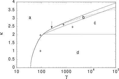
FIG. 10.: Phase diagram for the potential $V(y)=\theta(\kappa-y)$ in the $(\gamma,\kappa)$ plane for high $T$ by numerical maximization of the free energy Eq. (472) with the ansätze described in this section. The full lines separate phases with different types of global maxima. The RS, $1$-RSB, SG-IV, and SG-I phases are indicated by a, b, c, and d, respectively. The AT curve is the RS phase boundary for $\kappa<\kappa_{2}\simeq 2.38$ and to the right of the arrow it analytically continues in the dashed line, no longer a phase boundary. Reprinted from Ref. [17].

It is a plausible conjecture that the RS phase is obtained by analytic continuation from the phase of perfect storage below capacity $\alpha<\alpha_{\mathrm{c}}(\kappa)$. So although at high temperatures there is no phase with zero error, the analog phase is the one with RS (labeled by a). Note that at high $T$ we lost the intuitive picture, valid at $T=0$, that increasing $\kappa$ takes us into the frustrated phase. We obtain three RSB phases. One is $1$-RSB (b), the other the classic Parisi CRSB (SG-I, labeled by d), the third one is also CRSB, but with an extra plateau (SG-IV, labeled by c). The characteristic shapes for the OPF are shown in Fig. 11, note the plateau in the SG-IV phase (c).

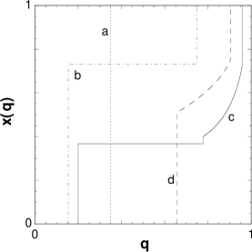
FIG. 11.: The $x(q)$ function at representative points as marked on Fig. 10 by crosses. Reprinted from Ref. [17].

Extensive thermodynamical quantities are shown on Fig. 12 for $\kappa=0$. The entropy is negative and decreases as it should for increasing $\alpha$, i. e., increasing $\gamma$. The mean error per pattern in the high-$T$ limit is $\frac{1}{2}$, and our approximation tells the correction $\varepsilon_{1}=T(\frac{1}{2}-\varepsilon)$ from the formula (486). For $\gamma\to\infty$ we expect that even the correction $\varepsilon_{1}$ vanishes, this is indeed suggested by the picture. The transition from RS to CRSB is of third order from the viewpoint of the free energy, i. e., its third derivative exhibits a discontinuity.

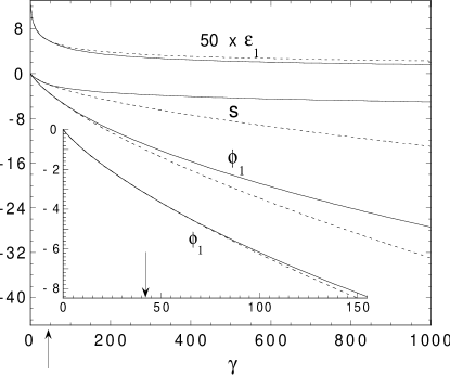
FIG. 12.: The entropy $s$, in leading order $s_{0}$ from Eq. (487), the free energy term $\phi_{1}$ from Eq. (472), and the enlarged correction $\varepsilon_{1}$ of the energy (486) in the high $T$ limit, for $\kappa=0$. The RS—SG-I transition is marked by an arrow. The dashed lines correspond to the thermodynamically unstable RS state beyond this transition point. The inset demonstrates the smoothness of the transition. Reprinted from Ref. [17].

If at $T=0$ the region beyond capacity is a single CRSB phase (SG-I), for $T\to\infty$ the decomposition into three different phases suggests singular surfaces born at finite $T$-s, whose precise locations we did not determine. For $\kappa<2$ the transition from RS to CRSB SG-I is of similar type as at $T=0$, but for $\kappa>2$ we have a transition from RS into $1$-RSB that does not have a counterpart at $T=0$. Nevertheless, the main picture, namely, that for low $\alpha$-s (translates into low $\gamma$-s here), there is a normal phase analog to a paramagnet, and for large $\alpha$-s the system exhibits complex, i. e., spin-glass-like behavior, is captured in the high-$T$ limit.

3 Numerical evaluation method for arbitrary temperatures^∗

As demonstrated in Sect. VII A 2, the maximization of $f[x(q)]$ with respect to $x(q)$ in (415) is done with the side conditions that $f(q,y)$ satisfies the PPDE (390) and $P(q,y)$ the SPDE (VII A 1). We further recall that $x(q)\equiv 0$ for $q<q_{(0)}$ and $x(q)\equiv 1$ for $q>q_{(1)}$, and that in the remaining non-trivial regime $q_{(0)}\leq q\leq q_{(1)}$ it is convenient to use for $x(q)$ the parametrization by $\xi(t)$ from (490).

For an actual numerical implementation, $\xi(t)$ has to be rewritten once more in the form of some ansatz with a finite number $N$ of variational parameters $v_{1},...,v_{N}$:

$$\xi(t)=\xi(t;v_{1},...,v_{N})\ .$$ (552)

For instance, $v_{1},...,v_{N}$ may be the coefficients of a polynomial ansatz for $\xi(t)$. Another option would be a piecewise linear ansatz with $v_{n}=\xi(t=(n-1)/(N-1))$. Also a finite-step RSB ansatz with the steps and plateaus parametrized by the $v_{n}$ is possible. Given any such parametrization (552), we are left with maximizing the free energy functional with respect to the $N+2$ variational parameters

$$v = (v_{0},v_{1},...,v_{N+1})$$ (554)

$$v_{0} = q_{(0)}$$ (555)

$$v_{N+1} = \eta=\beta(1-q_{(1)})\ ,$$ (556)

where we have expressed $q_{(1)}$ through $\eta$ according to (491). This maximization of the free energy functional $f[\mbox{\boldmath$v$}]$ has to be performed under the (non-holonomous) constraints $x(q_{(0)})\geq 0$, $x(q_{(1)})\leq 1$, and $\dot{x}(q)\geq 0$ for $q_{(0)}\leq q\leq q_{(1)}$, or equivalently, $\xi(0)\geq 0$, $\xi(1)/\beta\dot{q}(1)\leq 1$ (cf. (490)), and $\dot{\xi}(t)\dot{q}(t)-\xi(t)\ddot{q}(t)\geq 0$ for $1\leq t\leq 1$ (cf. (504)). It is convenient to incorporate these constraints into an augmented free energy functional $f_{\mu}(\mbox{\boldmath$v$})$ in the form of soft penalty terms:

$$f_{\mu}(\mbox{\boldmath$v$}) = f[\mbox{\boldmath$v$}]-\mu_{0}\psi(-\xi(0))-\mu_{t}\int_{0}^{1}{\mathrm{d}}t\,\psi(\xi(t)\ddot{q}(t)-\dot{\xi}(t)\dot{q}(t))$$ (559)

$$-\mu_{1}\psi(\xi(1)/\beta\dot{q}(1)-1)$$

$$\psi(x) = x^{2}\theta(x)/2\ .$$ (560)

Thus, by successively increasing the coefficients $\mu_{0}$, $\mu_{t}$, and $\mu_{1}$ in the course of the maximization procedure of $f_{\mu}(\mbox{\boldmath$v$})$, the respective constraints will be respected more and more rigorously.

Before we proceed, the following points are worth mentioning: (i) Like in Section VII A 9, our only assumption on $q(t)$ is that it should be a monotonically increasing function with $q(0)=q_{(0)}$ and $q(1)=q_{(1)}$. But for concrete numerical calculations, especially at low temperatures $T=\beta^{-1}$, the specific choice (489) has proven to be particularly appropriate. In any case, the implicit dependence of $q(t)$ on the variational parameters $v_{0}=q_{(0)}$ and $v_{N+1}=\eta$ should be kept in mind:

$$q(t)=q(t;v_{0},v_{N+1})\ .$$ (561)

(ii) In our experience, the maximization procedure typically ends not at the border of the admitted parameter-regime, where the soft constraints (559) come into action, but rather in the interior of this admitted region. However, in the course of the maximization this border may be visited, and, in the absence of the soft constraints in (559), the maximization procedure often goes out of the admitted region and diverges eventually. (iii) Strictly speaking, there are additional constraints on $v_{0}$ and $v_{N+1}$ associated with the restrictions $0\leq q_{(0)}<q_{(1)}\leq 1$; in our experience they, however, were never in danger to be violated with the obvious exception of cases with a stable RS solution. (iv) As in any variational ansatz, the necessary number $N$ of parameters depends on how well the ansatz is adapted to the problem. In principle, a polynomial or piecewise linear ansatz (552) with a sufficiently large number $N$ of parameters can approximate any shape of $x(q)$ arbitrarily well. Whether or not $N$ is sufficiently large in a given case should follow from the accuracy with which the stationarity conditions (420, 421) are satisfied. In practice, unavoidable numerical inaccuracies make things more complicated. As has been observed already in Ref. [16] within a 2-RSB ansatz, in the neighborhood of its maximum the free energy functional $f_{\mu}(\mbox{\boldmath$v$})$ changes extremely little upon certain parameter-variations, that is, the energy landscape $f_{\mu}(\mbox{\boldmath$v$})$ is very “flat” in certain directions. In our experience, with increasing number of parameters $N$ in (552), this problem becomes worse and worse in that the finite numerical accuracy gives rise to a spurious “roughness” in the already very “flat” energy landscape. As a consequence, any maximization strategy becomes slow or even fails for too large $N$. Similarly, the stability conditions are satisfied very well (in comparison with their numerical uncertainty) within a fairly large neighborhood of the true maximizing $x(q)$. As a consequence, in any specific case, a carefully tailored ansatz with not too many parameters has to be used and the criterion for convergence should be that $q_{(0)}$, $\eta$, and $\xi(t)$ change negligibly upon refining the parametrization (552).

In order to maximize the augmented free energy functional (559), a good compromise between robustness against the spurious numerical fine structure in the energy landscape and speed of convergence turned out to be a plain steepest descent procedure along the following lines: given a “working” parameter set $v$, the direction of the steepest increase of $f_{\mu}(\mbox{\boldmath$v$})$ is along the gradient $\partial f_{\mu}(\mbox{\boldmath$v$})/\partial\mbox{\boldmath$v$}$. Taking into account all the implicit dependencies on $v$ in (552), (561) and the expression (419) for the gradient of the original free energy functional, a straightforward but somewhat tedious calculation yields for the gradient of $f_{\mu}(\mbox{\boldmath$v$})$ from (559) the result

$$\frac{\partial f_{\mu}}{\partial v_{0}} = \int_{0}^{1}\frac{\dot{F}(t)\xi(t)}{2\dot{q}(t)}\frac{\partial q(t)}{\partial q_{(0)}}\,{\mathrm{d}}t+\frac{M_{1}}{\dot{q}(1)}\,\frac{\partial\dot{q}(1)}{\partial q_{(0)}}$$ (564)

$$-\int_{0}^{1}M(t)\left(\xi(t)\frac{\partial\ddot{q}(t)}{\partial q_{(0)}}-\dot{\xi}(t)\frac{\partial\dot{q}(t)}{\partial q_{(0)}}\right)\,{\mathrm{d}}t$$

$$\frac{\partial f_{\mu}}{\partial v_{n}} = \int_{0}^{1}\frac{F(t)}{2}\frac{\partial\xi(t)}{\partial v_{n}}\,{\mathrm{d}}t+\mu_{0}\,\psi^{\prime}(-\xi(0))\frac{\partial\xi(0)}{\partial v_{n}}-\frac{M_{1}}{\xi(1)}\,\frac{\partial\xi(1)}{\partial v_{n}}$$ (566)

$$-\int_{0}^{1}M(t)\left(\frac{\partial\xi(t)}{\partial v_{n}}\ddot{q}(t)-\frac{\partial\dot{\xi}(t)}{\partial v_{n}}\dot{q}(t)\right)\,{\mathrm{d}}t$$

$$\frac{\partial f_{\mu}}{\partial v_{N+1}} = \frac{F(1)}{2}-\int_{0}^{1}\frac{\dot{F}(t)\xi(t)}{2\beta\dot{q}(t)}\frac{\partial q(t)}{\partial q_{(1)}}\,{\mathrm{d}}t-\frac{M_{1}}{\beta\dot{q}(1)}\,\frac{\partial\dot{q}(1)}{\partial q_{(1)}}$$ (568)

$$-\int_{0}^{1}M(t)\left(\dot{\xi}(t)\frac{\partial\dot{q}(t)}{\beta\partial q_{(1)}}-\xi(t)\frac{\partial\ddot{q}(t)}{\beta\partial q_{(1)}}\right)\,{\mathrm{d}}t\,$$

where $1\leq n\leq N$, $\psi^{\prime}(x)=x\,\theta(x)$, we have introduced the quantities

$$M_{1} = \mu_{1}\,\psi^{\prime}(\xi(1)/\beta\dot{q}(1)-1)\,\xi(1)/\beta\dot{q}(1),$$ (570)

$$M(t) = \mu_{t}\,\psi^{\prime}(\xi(t)\ddot{q}(t)-\dot{\xi}(t)\dot{q}(t)),$$ (571)

and used $F(t)$ to denote the l. h. s. of Eq. (505) for a given $\xi(t)$ function.

Along the direction $\partial f_{\mu}(\mbox{\boldmath$v$})/\partial\mbox{\boldmath$v$}$ of steepest increase, one now searches for the maximum, i.e., the expression $f_{\mu}(\mbox{\boldmath$v$}+\lambda\,\partial f_{\mu}({\bf v})/\partial\mbox{\boldmath$v$})$ has to be maximized with respect to $\lambda$. This implies the condition

$$J(\lambda_{{\rm max}})=0$$ (572)

for the maximizing $\lambda=\lambda_{{\rm max}}$, where

$$J(\lambda)=\frac{\partial f_{\mu}(\mbox{\boldmath$v$}+\lambda\,\partial f_{\mu}(\mbox{\boldmath$v$})/\partial\mbox{\boldmath$v$})}{\partial\mbox{\boldmath$v$}}\cdot\frac{\partial f_{\mu}(\mbox{\boldmath$v$})}{\partial\mbox{\boldmath$v$}}\ .$$ (573)

By updating the parameter set as

$$\mbox{\boldmath$v$}\mapsto\mbox{\boldmath$v$}+\lambda_{{\rm max}}\,\partial f_{\mu}(\mbox{\boldmath$v$})/\partial\mbox{\boldmath$v$}$$ (574)

one completes one iteration step of the steepest descent procedure. This iteration scheme is then repeated until $v$ does not appreciably change any more. Note that due to the numerical inaccuracies it makes little sense to locate the zero from (572) very precisely in each iteration step. Our usual strategy was based on the assumption that $J(\lambda)$ behaves approximately linear near its zero at $\lambda=\lambda_{{\rm max}}$. If $J(\lambda)$ is given at two nearby $\lambda$-values, one then obtains an approximation for $\lambda_{{\rm max}}$ by linear interpolation. One such readily available $J(\lambda)$-value is that for $\lambda=0$, the second one follows by choosing for $\lambda$ the approximation for $\lambda_{{\rm max}}$ from the previous iteration step.

4 The CRSB state

In Ref. [18] we presented some characteristic results, obtained by the method expounded in the previous section, for the error measure (529). In a non-exhaustive search we found that if the RS solution is AT-unstable, at $T=0$ beyond capacity and also for some low temperatures, only a classic Parisi CRSB state emerges. Its OPF is given in 140), and also denoted as SG-I. We conjecture that at $T=0$ the region beyond capacity is such a phase. Sufficiently high $T$-s, where the $1$-RSB and the CRSB state with a plateau (SG-IV) would have arisen, as described in Section VII B 2, were not reached in our explorations.

The scaling introduced in Section VII A 9, and notably the introduction of the OPF $\xi(q)=\beta\,x(q)$, allows the description of the CRSB state at any temperatures, at the same time maintaining a smooth transition to the ground state, $T=0$. Physically, the fact that $x(q)\to 0$, at $T=0$, for any $q<1$ means that $q=1$ with probability one. Thus freezing sets in, similarly to the ground state of the SK model [29]. At the same time, the degenerate $x(q)$ is no longer a useful OPF, because the free energy becomes a functional of rather $\xi(q)$.

On Fig. 13 the scaled OPF $\xi(q)=\beta\,x(q)$ is displayed for various parameters.

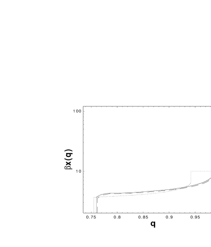
FIG. 13.: Scaled order parameter function $x(q)$ for $\kappa=0$, $\alpha=3$ at $T=0$ (solid), $T=0.01$ (dashed), and $T=0.1$ (dotted). The first discontinuity is at $q_{(0)}$, below the function is constantly zero. The second discontinuity for $T>0$ is $q_{(1)}$, which goes to $1$ for $T\to 0$. Reprinted from Ref. [18]

All parameter settings are in the AT-unstable region. This figure is the first indication, to our knowledge, of Parisi’s CRSB state for low temperatures in a system that is not a model of long range interaction spin glasses, or closely related to such as the Little-Hopfield network. It is remarkable that the scaling by $\beta$ makes the continuously increasing segment $\xi_{c}(q)=\beta\,x_{c}(q)$ of the OPF little sensitive to the temperature. Equally stable is the lower end $q_{(0)}$ of the $\xi_{c}(q)$ segment, but the upper end $q_{(1)}$ shows linear temperature dependence, $1-q_{(1)}\propto T$. The rightmost plateau’s value is obviously $\xi(1)=\beta$.

At the same parameter settings as before the local stability density is displayed on Fig. 14.

FIG. 14.: Density of local stabilities $\rho(\Delta)$ from theory for $\kappa=0$, $\alpha=3$ at $T=0$ (solid), $T=0.01$ (dashed), and $T=0.1$ (dotted). Reprinted from Ref. [18]

Since in the method of Section VII B 3 the evaluation of the probability field $P(q,y)$ by the scaled SPDE (499) is done in every approximant step, we obtain the sought field in the end by (510). Not shown is the Dirac delta peak at $T=0$, this restores normalization to one there. A gap exists at $T=0$, with right border $\Delta=\kappa$, in accordance with (533), but the gap immediately disappears for any positive $T$, as it can be seem from (510). At $T=0$ the density $\rho(\Delta)$ linearly vanishes at the lower edge of the gap.

Comparison between the CRSB solution and earlier RS [5], $1$-RSB [7, 8], and $2$-RSB [11] approaches shows that averaged quantities, like the mean error per pattern do not show significant differences. The qualitative behavior of the error, that it is zero below and is positive beyond capacity at $T=0$, furthermore that it linearly increases for small $\alpha-\alpha_{c}$, is reflected by the previous solutions. The $1$- and $2$-RSB $\varepsilon(\alpha)$ curves look the same on a resolution of a figure [11]. On the other hand, the difference is more conspicuous in the distribution of non-self-averaging quantities. The OPF $x(q)$ is the averaged probability measure of the overlap of coupling vectors, and the definitely continuously increasing part of it in Figs. 13, 11 shows that finite $R$-RSB-s are qualitatively in error. Further qualitative difference can be found in the distribution of local stabilities $\rho(\Delta)$. Indeed, for finite $R$-RSB the $\rho(\Delta)$ exhibits a discontinuity at the lower edge of the gap. The right tendency is shown by the feature that the size of the discontinuity is smaller in the $1$-RSB than in the RS solution [7].

5 Simulation

In this section we describe the simulation results from [18]. Wendemuth adapted existing algorithms for below capacity of the simple perceptron, with potentials of the form (35), to the region beyond it by specially dealing with patterns with positive stabilities [154], and performed a series of simulations [37]. The most sensitive part of his work was on the potential with $b=0$, which counts the number of unstable patterns, an NP-complete problem from the algorithmic viewpoint [153]. His data showed significant deviation from the then available best theoretical prediction from the $1$-RSB calculation of Majer, Engel, and Zippelius [7]. He evaluated the probability density of local stabilities at $\alpha=1$ and $\kappa=1$, a point known to be beyond capacity. Although the shapes roughly resembled, a gap, and a peak at its right end, were present, the simulation data gave systematically and discouragingly larger stabilities than predicted by theory.

Essentially following Wendemuth’s algorithm we redid the simulation in order to see how persistent the deviation is. The first step is to generate random patterns (26). We selected numbers with uniform distribution from an interval centered around zero and in the end normalized them as

$$\sum_{k=1}^{N}(S^{\mu}_{k})^{2}=N$$ (575)

The output for the patterns, $\xi^{\mu}$, were taken uniformly $1$, not restricting generality, for $S^{\mu}_{k}$ have random signs. The algorithm goes in discrete time $t=0,1,\dots$. We initialized at $t=0$ the coupling vector according to the Hebb rule

$$J_{k}(0)=\text{const.}\,\sum_{\mu=1}^{M}S_{k}^{\mu},$$ (576)

with the constant chosen so that the Eucledian norm was $|\mbox{\boldmath$J$}(0)|=N$. At time $t$ the local stabilities

$$\Delta^{\mu}(t)=\frac{\mbox{\boldmath$J$}(t)\cdot\mbox{\boldmath$S$}^{\mu}}{|\mbox{\boldmath$J$}(t)|}$$ (577)

are computed and among the unstable ones, i. e., $\Delta^{\mu}(t)<\kappa$, the one with the largest $\Delta^{\mu}(t)$ is selected. This is the least unstable pattern, characterized by the index $\mu_{0}(t)$. The couplings are updated according to the rule of Wendemuth [154, 37]. We took

$$\mbox{\boldmath$J$}(t+1)=\mbox{\boldmath$J$}(t)+\lambda\left(\mbox{\boldmath$S$}^{\mu_{0}(t)}+\Delta\mbox{\boldmath$S$}(t)\right),$$ (578)

where

$$\Delta\mbox{\boldmath$S$}(t)=\left\{\begin{array}[]{ll}0&\quad\text{if~{}}\Delta^{\mu_{0}(t)}(t)>0\\ \mbox{\boldmath$J$}(t)\frac{N/|\mbox{\boldmath$J$}(t)|-\Delta^{\mu_{0}(t)}(t)}{|\mbox{\boldmath$J$}(t)|-\Delta^{\mu_{0}(t)}(t)}&\quad\text{if~{}}\Delta^{\mu_{0}(t)}(t)<0.\end{array}\right.$$ (579)

The $\lambda$ is the gain parameter, chosen in Ref. [154] as $\lambda=N^{-3/2}$. By trial and error we found that a larger gain parameter $\lambda=N^{-1}$ did not endanger overall convergence, and made the final approach for a given pattern, $\Delta^{\mu_{0}(t)}(t)\to\kappa$, faster. The second row in the update rule (579) is Wendemuth’s term introduced to specially cope with patterns with negative stability.

At the next time step $t+1$ we again find the least unstable pattern with index $\mu_{0}(t+1)$ and update the couplings by the above rule. The usual course of the algorithm is that the least unstable pattern is the same, $\mu_{0}(0)=\mu_{0}(1)=\dots$, until it becomes stabilized at say $t_{1}-1$, whence another pattern is taken for some steps, $\mu_{0}(t_{1})=\mu_{0}(t_{1}+1)=\dots$, again until it becomes stabilized. In principle, another pattern may become least stable before the one in question is stabilized, but typically this was not the case.

The above recipe is repeated until a pattern cannot be stabilized in a reasonable time. The notion of reasonable time could be quantified, because the time needed to stabilize a pattern showed a systematic increase as function of the total number of patterns stabilized before. Therefore, it is a good recipe to halt the algorithm, when a pattern cannot be stabilized within a small multiple of the extrapolated convergence time. In test runs, if the last pattern could not be stabilized within twice the extrapolated convergence time, it could not within ten times of the same either. Thus we are confident that we exploited the possibilities of the update rule described above.

Wendemuth algorithm is based on the argument that one has the highest chance to stabilize the pattern among all patterns with $\Delta^{\mu}<\kappa$ whose $\Delta^{\mu}$ is closest to $\kappa$. So this algorithm may maximize the number of stable patterns, by successively pushing the stability of the least unstable pattern to $\kappa$ from below. A consequence is that the remaining non-stabilized patterns with $\Delta^{\mu}<\kappa$ will have relatively large distance $\kappa-\Delta^{\mu}$, but the latter quantity does not enter the present error measure. Nevertheless, the principle of stabilizing the least unstable pattern resembles qualitatively the gradient descent algorithm for differentiable error measures, because every step is made in the momentarily most promising direction. The shortcomings of such algorithms in NP-complete problems is known, and we cannot be certain that the number of unstable patterns is indeed minimized.

The result of the simulation at the parameter setting $\alpha=\kappa=1$ is shown on Fig. 15. Since $\kappa>0$, in the final approach $\Delta^{\mu_{0}(t)}\to\kappa$ for the momentarily least unstable pattern the stability is positive, so the second row in the update rule (579) does not come into play.

FIG. 15.: Density of local stabilities $\rho(\Delta)$ at $\alpha=\kappa=1$. The horizontal axis is $\Delta$, the vertical one $\rho$. The theoretical prediction is given by the full line. The two empirical densities are normalized histograms, taken with $M=N=500$ and $1000$. Reprinted from Ref. [18].

The full line is the result of numerical extremization of the variational free energy (416) by the method explained in Section VII B 3. We omitted the Dirac delta peak of the theoretical probability density at $\kappa=1$. The dashed lines are the histograms for the local stabilities from simulation for two sizes, $M=N=500$ and $1000$, with proper normalization. We do not enclose the original data of Wendemuth [37], but mention that his histogram showed a much larger systematic error. To quantify the deviation let us consider the mean error $\varepsilon$, i. e., the relative number of misclassified patterns. Wendemuth’s number is $0.21$, the present simulation gives $0.15$, while theory predicts $0.1358$. Thus we are still about $10\%$ off the theoretical value, but it is a remarkable improvement w. r. t. the previous deviation of $55\%$. The size of the gap from simulation is also within about $10\%$ of the theoretical value. The simulation data reproduces, for the larger size $M=N=1000$, the property that the density $\rho(\Delta)$ linearly vanishes at the lower edge of the gap. This should be contrasted with the $1$-RSB result in Ref. [7], where the size of the discontinuity at the lower edge of the gap is about the third of the height of left peak. The simulation clearly favors the CRSB solution.

In summary, the theoretical and simulation data do not match perfectly, however, given the NP-completeness of the numerical problem, this does not disprove theory. We mention that the algorithm used had the primitive side of being deterministic, furthermore, it does not have a rigorous mathematical basis for convergence to the desired state. There is obviously room for further improvements.

VIII The Neuron: Independently Distributed Synapses

A Free energy and stationarity condition

In this paper we focus mostly on the spherical neuron. Since, however, the main formulas for the case of prior distribution (32), where synapses are independent and obey arbitrary distribution, follow straightforwardly from Section IV, we now briefly review them. In the course of continuation the limits

$$q_{0}\to q_{(0)}~{} ~{}~{}~{}q_{R}\to q_{(1)},$$ , (581)

$$\hat{q}_{0}\to\hat{q}_{(0)}~{} ~{}~{}~{}\hat{q}_{R}\to\hat{q}_{(1)}$$ , (582)

are assumed. The corresponding free energy (III C) can be characterized by two OPF-s

$$q(x)~{} ~{}~{}~{}q(0)=q_{(0)}~{},~{}~{}~{}q(1)=q_{(1)}~{},$$ , (584)

$$\hat{q}(x)~{} ~{}~{}~{}\hat{q}(0)=\hat{q}_{(0)}~{},~{}~{}~{}\hat{q}(1)=\hat{q}_{(1)}.$$ , (585)

Alternatively, we can take as OPF-s the respective inverses

$$x(q)~{},~{}~{}~{}\hat{x}(\hat{q})$$ (586)

Then

$$\hat{q}=\hat{q}(x(q)),$$ (587)

or its inverse function

$$q=q(\hat{x}(\hat{q}))$$ (588)

establishes a relation between the overlaps $q$ and $\hat{q}$.

Concerning the $f_{\mathrm{e}}$ term, Eqs. (388-VII A 1) from the spherical case carry over unchanged. The entropic term (62) is a transcript of (131) with (74) together with the appropriate equations that produce the averages. We introduce the field (see Eqs. (129,130)

$$\hat{f}(\hat{q},y)=-\beta^{-1}\hat{\varphi}(\hat{q},y)$$ (589)

to get

$$\hat{f}_{\mathrm{s}}[\hat{x}(\hat{q})]=\lim_{n\to 0}\frac{1}{n}\hat{f}_{\mathrm{s}}({\sf\hat{Q}})=-\beta^{-1}\left.\hat{\varphi}\left[\ln\int{\mathrm{d}}u~{}w_{0}(u)~{}e^{-\beta uy},{\sf\hat{Q}}\right]\right|_{n=0}=\hat{f}(0,0),$$ (590)

where $\hat{f}(\hat{q},y)$ is the solution of

$$\partial_{\hat{q}}\hat{f} = -\frac{1}{2}\partial_{y}^{2}\hat{f}+\frac{1}{2}\beta\hat{x}\left(\partial_{y}\hat{f}\right)^{2},$$ (592)

$$\hat{f}(\hat{q}_{(1)},y) = -\beta^{-1}\ln\int{\mathrm{D}}z\int{\mathrm{d}}u~{}w_{0}(u)~{}e^{-\beta u(y+iz\sqrt{\hat{q}_{(1)}})}.$$ (593)

Introducing

$$\hat{m}(\hat{q},y)=\partial_{y}\hat{f}(\hat{q},y),$$ (594)

we have

$$\partial_{\hat{q}}\hat{m} = -\frac{1}{2}\partial_{y}^{2}\hat{m}+\beta\hat{x}\hat{m}\partial_{y}\hat{m},$$ (596)

$$\hat{m}(\hat{q}_{(1)},y) = \partial_{y}\hat{f}(\hat{q}_{(1)},y).$$ (597)

Furthermore, the $\hat{~{}}$-ed ’susceptibility field’ is

$$\hat{\chi}(\hat{q},y)=\partial_{y}\hat{m}(\hat{q},y),$$ (598)

obeying

$$\partial_{\hat{q}}\hat{\chi} = -\frac{1}{2}\partial_{y}^{2}\hat{\chi}+\beta\hat{x}(\hat{m}\partial_{y}\hat{\chi}+\hat{\chi}^{2}),$$ (600)

$$\hat{\chi}(\hat{q}_{(1)},y) = \partial_{y}^{2}\hat{f}(\hat{q}_{(1)},y).$$ (601)

The probability density $\hat{P}(\hat{q},y)$ satisfies a variant of the SPDE

$$\partial_{\hat{q}}\hat{P} = \frac{1}{2}\partial_{y}^{2}\hat{P}+\beta\hat{x}\partial_{y}(\hat{P}\hat{m}),$$ (603)

$$\hat{P}(0,y) = \delta(y).$$ (604)

The interaction term (61) is simplest if expressed through the functions (VIII A)

$$f_{i}[x(q),\hat{x}(\hat{q})]=-\beta\int_{0}^{1}{\mathrm{d}}x~{}q(x)~{}\hat{q}(x).$$ (605)

Since a function is a functional of its inverse, the $f_{i}[\dots]$ can be considered as functional of $x(q)$ and $\hat{x}(\hat{q})$.

The stationarity conditions (64,65) now read as

$$q = \int{\mathrm{d}}y~{}\hat{P}(\hat{q},y)~{}\hat{m}(\hat{q},y)^{2},$$ (607)

$$\hat{q} = \alpha\int{\mathrm{d}}y~{}P(q,y)~{}m(q,y)^{2},$$ (608)

where the connection between $q$ and $\hat{q}$ is established by (587) or (588). The r. h. sides are respective functionals of $\hat{x}(\hat{q})$ and $x(q)$. Note that solving these equations involves also finding the starting point $\hat{q}_{(1)}$, in contrast to the evaluation of the energy term, where the initial condition is fixed at $q=1$. Given the solution for the stationary $x(q)$ and $\hat{x}(\hat{q})$, by substituting them into the r. h. s. of

$$f=\hat{f}_{\mathrm{s}}[\hat{x}(\hat{q})]+f_{i}[x(q),\hat{x}(\hat{q})]+\alpha f_{\mathrm{e}}[x(q)]$$ (609)

we obtain the final result for the mean free energy.

A special case of independently distributed synapses is the clipped neuron, i. e., the neuron with discrete synapses. The most studied such model is the Ising neuron with binary synapses, which has attracted considerable interest (see [19] and [12] for references). The prior distribution in the Ising case involves (33), so the initial conditions for the PDE-s are

$$\hat{f}(\hat{q}_{(1)},y) = -\beta^{-1}\ln\text{cosh}\beta y+\frac{1}{2}\beta\hat{q}_{(1)},$$ (611)

$$\hat{m}(\hat{q}_{(1)},y) = -\text{tanh}\beta y.$$ (612)

The Ising neurons studied in the literature so far were reminiscent to the random energy model in that they involved at most $1$-RSB [231]. However, only a few choices of the error measure potential $V(y)$ were considered, and at this stage it cannot be excluded that the full Parisi scheme becomes of import for other potentials.

Finally we emphasize that previously studied SK-type spin glasses, with Ising, or, as a matter of fact, any kind of individual spin constraint (32), are included in the considerations of this section. Formulae equivalent with (VIII A) are well known from the SK model. This is not surprising, because the entropic term with the Ising constraint is the same for both the SK spin glass and the present neuron model. In the case of other constraints for the SK-type spin glass the first two terms on the r. h. s. of (609) remain valid. Concerning the third, the energy term, let us assume the most general multi-spin interaction of Nieuwenhuizen’s [68] resulting in a term (373). Then indeed, if in (609) the $\alpha f_{\mathrm{e}}$ is replaced by the energy term (376), with the understanding of the correspondence (374,375), one obtains by (609) the full free energy functional of the spin glass problem.

B Variational principle

The results of Section VIII A can also be derived from a variational principle. A reasoning similar to what we followed in the spherical problem yields a free energy functional $f[\dots]$ that produces the mean free energy as

$$f={\begin{array}[]{c}\mbox{~{}}\\ \mbox{max}\\ \mbox{{\em x(q)}}\end{array}}{\begin{array}[]{c}\mbox{ ~{}}\\ \mbox{extr}\\ \mbox{{\em f(q,y),P(q,y)\,}}\end{array}}\!\!\!{\begin{array}[]{c}\mbox{~{}}\\ \mbox{extr}\\ \mbox{{$\,\hat{x}(\hat{q})$}}\end{array}}{\begin{array}[]{c}\mbox{ ~{}}\\ \mbox{extr}\\ \mbox{{$\hat{f}(\hat{q},y),\hat{P}(\hat{q},y)$}}\end{array}}\!\!\!f\left[x(q),f(q,y),P(q,y),\hat{x}(\hat{q}),\hat{f}(\hat{q},y),\hat{P}(\hat{q},y)\right].$$ (613)

The order of the extremum conditions is not binding, but, given the physical meaning of the OPF $x(q)$, the maximum is to be taken last. The free energy functional is

$$f[\dots] = \hat{f}_{\mathrm{s}}[\dots]+\hat{f}_{a}^{(1)}[\dots]+\hat{f}_{a}^{(2)}[\dots]+f_{i}[\dots]+\alpha(f_{\mathrm{e}}[\dots]+f_{a}^{(1)}[\dots]+f_{a}^{(2)}[\dots]),$$ (615)

$$\hat{f}_{\mathrm{s}}[\dots] = \hat{f}(0,0),$$ (616)

$$\hat{f}_{a}^{(1)}[\dots] = \int_{0}^{\hat{q}_{(1)}}\!\!{\mathrm{d}}\hat{q}\ \int{\mathrm{d}}y~{}\hat{P}(\hat{q},y)\left[\partial_{\hat{q}}\hat{f}(\hat{q},y)+\frac{1}{2}\partial_{y}^{2}\hat{f}(\hat{q},y)-\frac{1}{2}\beta\hat{x}(\hat{q})\left(\partial_{y}\hat{f}(\hat{q},y)\right)^{2}\right],$$ (617)

$$\hat{f}_{a}^{(2)}[\dots] = -\int{\mathrm{d}}y~{}\hat{P}(\hat{q}_{(1)},y)\left[\frac{1}{\beta}\ln\int{\mathrm{d}}u~{}w_{0}(u)~{}e^{-\beta uy}+\hat{f}(\hat{q}_{(1)},y)\right],$$ (618)

where $f_{\mathrm{e}}[\dots]$, $f_{a}^{(1)}[\dots]$, $f_{a}^{(2)}[\dots]$, and $f_{i}[\dots]$ are given by Eqs. (426), (427), (428), and (605), respectively. The remarkable symmetry of the above expressions in the quantities with and without the $~{}\hat{}~{}$ mark is the consequence of the fact that both the entropic and the energy terms are essentially of the general Parisi form, the main difference being in the starting point of the time variable and the initial condition for the PDE.

The free energy functional $f[\dots]$ should be maximized in $x(q)$ and extremized over the other function arguments. Besides the extremization of terms analogous to those appearing in Section VII A 3, we have to calculate the functional derivatives of $f_{i}[x(q),\hat{x}(\hat{q})]$. If $u^{-1}(u)$ is the inverse of some function $u(t)$ then variation of the identity $u^{-1}(u(t))=t$ yields the functional derivative of the inverse function as

$$\frac{\delta\,u^{-1}(u(t_{1}))}{\delta\,u(t_{2})}=-\frac{\delta(t_{2}-t_{1})}{\dot{u}(t_{1})}.$$ (619)

This relation helps us to calculate the sought derivatives of the interaction term

$$\frac{\delta\,f_{i}[x(q),\hat{x}(\hat{q})]}{\delta\,x(q)}=\beta\,\hat{q}(x(q))$$ (621)

$$\frac{\delta\,f_{i}[x(q),\hat{x}(\hat{q})]}{\delta\,\hat{x}(\hat{q})}=\beta\,q(\hat{x}(\hat{q})).$$ (622)

These, together with functional derivatives of the type determined in Section VII A 3, lead to the stationarity relations displayed in Section VIII A for intervals of strictly increasing OPF-s, including the points where the OPF-s exhibit a step. Plateaus should be dealt with in a manner similar to what was described in Section VII A 3. Extremization in terms of the starting point in time of the $\hat{~{}}$-ed PDE, $\hat{q}_{(1)}$, yields

$$\beta\,\hat{x}(\hat{q}_{(1)})\,q_{(1)}=\int{\mathrm{d}}y~{}\hat{P}(\hat{q}_{(1)},y)\,\hat{\chi}(\hat{q}_{(1)},y),$$ (623)

a condition which was not displayed in Section VIII A.

C On thermodynamical stability

In the case of independently distributed synapses the free energy (III C) involves combined maximization and extremization. Clearly, there are no stability requirements following from the ’extr’ condition. On a simple example we now give the recipe for stability calculations in the replicon sector for such a case.

Consider the two-variable function

$$F(x,\hat{x})=f(x)+\hat{f}(\hat{x})+x\hat{x},$$ (624)

where $f$ and $\hat{f}$ are real functions. We are seeking

$${\begin{array}[]{c}\text{~{}}\\ \text{min}\\ \text{$x$}\end{array}}{\begin{array}[]{c}\text{~{}}\\ \text{extr}\\ \text{$\hat{x}$}\end{array}}F(x,\hat{x}).$$ (625)

Extremum conditions for $x$ and $\hat{x}$ imposed simultaneously would read as

$$x = -\hat{f}^{\prime}(\hat{x}),$$ (627)

$$\hat{x} = -f^{\prime}(x).$$ (628)

Substitution of the stationary value (628) gives

$$F(x)\equiv F(x,-f^{\prime}(x))=f(x)+\hat{f}(-f^{\prime}(x))-xf^{\prime}(x).$$ (629)

The stationarity condition in terms of $x$ is

$$F^{\prime}(x)=-f^{\prime\prime}(x)\left[x+\hat{f}^{\prime}(-f^{\prime}(x))\right]=0.$$ (630)

The stationary point $x+\hat{f}^{\prime}(-f^{\prime}(x))=0$ is a minimum of $F(x)$, if

$$\left.F^{\prime\prime}(x)\right|_{x=-\hat{f}^{\prime}(-f^{\prime}(x))}=-f^{\prime\prime}(x)\left[1-\hat{f}^{\prime\prime}(\hat{x})f^{\prime\prime}(x)\right]>0,$$ (631)

where (627,628) are understood. If we have more-than-one-dimensional objects en lieu of $x$ and $\hat{x}$, and at the saddle the Hessian matrices of $f$ and $\hat{f}$ can be simultaneously diagonalized, then a similar formula holds, wherein the appropriate eigenvalues of the Hessian at stationarity should be substituted for $f^{\prime\prime}(x)$ and $\hat{f}^{\prime\prime}(\hat{x})$.

The above principle can be applied to the case of independently distributed synapses. There are two families of replicon eigenvalues, $\lambda_{\mathrm{e}}(q_{1},q_{2},q_{3})$ and $\hat{\lambda}_{\mathrm{s}}(\hat{q}_{1},\hat{q}_{2},\hat{q}_{3})$ coming from the energy and entropic term, respectively. The contribution from the energy term, $\lambda_{\mathrm{e}}(q_{1},q_{2},q_{3})$, is the same as in the spherical case, given by Eq. (433). Analogously, from the $\hat{~{}}$-ed entropic term we have

$$\hat{\lambda}_{\mathrm{s}}(\hat{q}_{1},\hat{q}_{2},\hat{q}_{3})=-\beta^{2}\int\,{\mathrm{d}}y_{2}\,{\mathrm{d}}y_{3}\,\hat{\Gamma}_{\varphi\varphi\varphi}\left(\hat{q}_{1};0,0;\hat{q}_{2},y_{2};\hat{q}_{3},y_{3}\right)\hat{\chi}\left(\hat{q}_{2},y_{2}\right)\,\hat{\chi}\left(\hat{q}_{3},y_{3}\right).$$ (632)

Here we spell out the obvious, namely, the $\hat{~{}}$-ed PPDE gives rise to a $\hat{~{}}$-ed Green function, see Section IV B 4, whence the vertex function $\hat{\Gamma}_{\varphi\varphi\varphi}$ can be defined. Finally, based on (631) the necessary criterion of stability becomes

$$-\lambda_{\mathrm{e}}(q_{1},q_{2},q_{3})\left[1-\alpha\lambda_{\mathrm{e}}(q_{1},q_{2},q_{3})\,\hat{\lambda}_{\mathrm{s}}(\hat{q}_{1},\hat{q}_{2},\hat{q}_{3})\right]\geq 0.$$ (633)

Here we have omitted a prefactor $\alpha$ and allowed equality for the sake of possible Goldstone modes in a Parisi phase. The stability condition is of course understood at stationarity, which yields a concrete $q=q(\hat{q})$ function. That implies $q_{i}=q(\hat{q}_{i})$, so the overall replicon eigenvalue is parametrized by three independent variables, as in the spherical case.

IX Conclusions and Outlook

The main messages of this paper were extensively discussed and conclusions were advanced in Chs. I and II, so we only highlight a few moral issues here.

A sensitive question in approximating a CRSB state by finite $R$-RSB is how good it will turn out to be in the end. However, there is so far no reliable a priori estimate of this error, as opposed to say a series expansion, where the last power retained gives at least asymptotically a bound for the error. Sometimes there is a qualitative indicator showing that a low order approximation is wrong. Long known example is the ground state entropy of the SK model, which was negative for finite $R$-RSB ansätze, a problem cured only by Parisi’s CRSB solution. However, often macroscopic quantities are quite well approximated with the RS or low $R$-RSB solution. The main advantage of the CRSB calculation w. r. t. the approximations is that the latter may not be able to even qualitatively correctly predict distributions of local, non-self-averaging quantities, like the overlaps and local fields. These are observables in numerical simulations and can help to decide between candidate theories (see, e. g., the numerical review [91] on spin glasses).

On the technical side, the mathematical framework discussed in Chs. IV, V, and VI relates to the general properties of CRSB phases, irrespective of the storage problem of the neuron, upon which its use was demonstrated subsequently. It allows for a non-perturbative description in a wide range of problems in disordered systems, like long range interaction spin glasses other than the SK model, and may be a starting point for the study of frustrated phases, i. e., unsatisfiable situations, in optimization problems in general.

Among the notoriously difficult problems in artificial neural networks is the problem of learning and generalization of unlearnable tasks [199, 232]. In the traditional scenario of equilibrium, i. e., batch, learning from examples, an unlearnable problem is characterized by the fact that there is a limited number of examples the network can reproduce. Beyond this limit of error-free learning, the generalization ability might be further improved, but the minimal training error is positive. This is in close analogy with the region beyond capacity in the storage problem, so it is a sensible assumption that theoretical methods able to deal with imperfect storage may also be of use for the description of learning the unlearnable. Further possible area of application is unsupervised learning [232], where no desired output is given, rather the properties of the distribution of examples is to be extracted. Again, if the network can be saturated by the examples a complex phase appears, where methods similar to those presented in this paper may be the key to the solution.

A Abbreviations

This Appendix lists acronyms and abbreviations used throughout the paper.

left-hand-side l. h. s. 
right-hand-side r. h. s. 
with respect to w. r. t. 
de Almeida-Thouless [stability]AT
Green functionGF
Order parameter function OPF
Partial differential equationPDE
Parisi’s PDE, Eq. (119) PPDE
Replica symmetry breakingRSB
$R$-step RSB$R$-RSB
Continuous RSBCRSB
Sherrington-Kirkpatrick [model] SK
Sompolinsky’s PDE, Eqs. (153,154) SPDE
Ward-Takahashi identityWTI

B Derivation of the replica free energy

The $n$-th moment of the partition function (36), with (27) inserted as constraint, reads as

$$\left<Z^{n}\right>=\int\prod_{a}{\mathrm{d}}^{N}\!J_{a}\ w(\mbox{\boldmath$J$}_{a})\prod_{\mu}{\mathrm{d}}y_{a}^{\mu}\ e^{-\beta V(y_{a}^{\mu})}\left<\delta\left(y_{a}^{\mu}-N^{-1/2}\xi^{\mu}\sum_{k}J_{ak}S_{k}^{\mu}\right)\right>.$$ (B1)

The indices $k$, $\mu$, and $a$ run from $1$ to $N$, $M$, and $n$, respectively. The Fourier transformation of the Dirac deltas introduces the ancillary variables $x_{a}^{\mu}$ adjoint to $y_{a}^{\mu}$. Average over the Gaussian distribution of patterns $S_{k}^{\mu}$, and over the outputs $\xi^{\mu}$, which are $\pm 1$ equally likely, can be performed straightforwardly. In fact, since $S_{k}^{\mu}$ is scaled by the vanishing factor $N^{-1/2}$, the same result would be obtained for other distributions of $\xi^{\mu}S_{k}^{\mu}$ with zero mean and unit variance independent of $\mu$ and $k$.

$$\left<Z^{n}\right> = \int\left[\prod_{a}{\mathrm{d}}^{N}\!J_{a}\ w(\mbox{\boldmath$J$}_{a})\,\prod_{\mu}\frac{{\mathrm{d}}x_{a}^{\mu}{\mathrm{d}}y_{a}^{\mu}}{2\pi}\right]$$ (B3)

$$\times\,\prod_{\mu}\exp\left(-\beta\sum_{a}V(y_{a}^{\mu})+\sum_{a}ix_{a}^{\mu}y_{a}^{\mu}-\frac{1}{2N}\sum_{a,b}x_{a}^{\mu}x_{b}^{\mu}\sum_{k}J_{ak}J_{bk}\right).$$

If we substitute the overlaps defined in (48), the product over $\mu$ gives the $M=\alpha N$-th power of $e^{-n\beta f_{\mathrm{e}}({\sf Q})}$, where $f_{\mathrm{e}}({\sf Q})$ is displayed in (47). Our inserting the constraint (48) yields

$$\left<Z^{n}\right>=\int\left[\prod_{a}{\mathrm{d}}^{N}\!J_{a}\ w(\mbox{\boldmath$J$}_{a})\right]\ e^{-N\alpha\beta f_{\mathrm{e}}({\sf Q})}\prod_{a<b}N{\mathrm{d}}q_{ab}\ \delta\left(Nq_{ab}-\sum_{k}J_{ak}J_{bk}\right).$$ (B4)

For both the spherical (III A) and the independent (see condition below (32)) prior distributions we have $q_{aa}\equiv q_{\mathrm{D}}=1$. Fourier transformation of the Dirac deltas introduces the variables $\tilde{q}_{ab}$ adjoint to $q_{ab}$, and we have

$$\left<Z^{n}\right> = \int\left[\prod_{a<b}\frac{N}{2\pi}{\mathrm{d}}q_{ab}\,{\mathrm{d}}\tilde{q}_{ab}\right]\left[\prod_{a}{\mathrm{d}}^{N}\!J_{a}\ w(\mbox{\boldmath$J$}_{a})\right]e^{-N\alpha\beta f_{\mathrm{e}}({\sf Q})}$$ (B6)

$$\times\,\exp\left(iN\sum_{a<b}q_{ab}\tilde{q}_{ab}-i\sum_{k}\sum_{a<b}\tilde{q}_{ab}J_{ak}J_{bk}\right).$$

We shall see that for the prior densities of interest, after integration by the synaptic coefficients, the exponential has the overall coefficient $N$. Then for $N\to\infty$ the saddle point method can be applied, and it will turn out that the stationary value of each $tilde{q}_{ab}$ is imaginary. We presume that the prior density is such that the integration path of $\tilde{q}_{ab}$ can be distorted so as to go through the imaginary saddle point. The path can then be taken a straight line parallel or perpendicular to the imaginary axis in a sufficiently large neighborhood of the saddle point, depending on which orientation ensures a maximum at the saddle. This procedure is typical if one integrates a fast oscillating integrand — then only an extremum, not specifically minimum, condition should be satisfied. If we succeed in determining the saddle values of the $\tilde{q}_{ab}$-s as function of the $q_{ab}$-s, we have to minimize in terms of $q_{ab}$. We shall see that this can be carried out for the spherical constraint (III A), but we cannot explicitly determine the $\tilde{q}_{ab}$-s for general independent synapses (32).

In the case of the spherical constraint (III A) we shall make use of the advance knowledge that the stationary values of $\bar{q}_{ab}=i\tilde{q}_{ab}$ are real. Let us insert the Fourier transform of the Dirac deltas representing the spherical constraints, thereby introducing the integration variables $\tilde{q}_{a}$, then switch over to $\bar{q}_{a}=i\tilde{q}_{a}$ to obtain

$$\left<Z^{n}\right> = C_{N}\,N^{\frac{n(n-1)}{2}}(2\pi)^{-\frac{n(n+1)}{2}}\int\left[\prod_{a<b}{\mathrm{d}}q_{ab}\,{\mathrm{d}}\bar{q}_{ab}\right]\left[\prod_{a}{\mathrm{d}}^{N}\!J_{a}\,{\mathrm{d}}\bar{q}_{a}\right]e^{-N\alpha\beta f_{\mathrm{e}}({\sf Q})}$$ (B8)

$$\times\exp\left(N\sum_{a<b}q_{ab}\bar{q}_{ab}+N\sum_{a}\bar{q}_{a}-\sum_{k,a}\bar{q}_{a}{J_{ak}}^{2}-\sum_{k}\sum_{a<b}\bar{q}_{ab}J_{ak}J_{bk}\right).$$

We can introduce diagonal elements for the matrix ${\sf\bar{Q}}$ as $\bar{q}_{aa}=2\bar{q}_{a}$. Performing the Gaussian integrals over $J_{ak}$ we obtain

$$\left<Z^{n}\right> = C_{N}\,N^{\frac{n(n-1)}{2}}(2\pi)^{\frac{n(N-n-1)}{2}}\,\int\left[\prod_{a<b}{\mathrm{d}}q_{ab}\right]\left[\prod_{a\leq b}{\mathrm{d}}\bar{q}_{ab}\right]$$ (B10)

$$\times\,\exp N\left(-\alpha\beta f_{\mathrm{e}}({\sf Q})+\frac{1}{2}\text{Tr}{\sf Q}{\sf\bar{Q}}-\frac{1}{2}\text{lndet}{\sf\bar{Q}}\right).$$

Given the asymptotics of the prefactor

$$\frac{\ln C_{N}}{N}\approx-\frac{1}{2}\ln 2\pi e,$$ (B11)

in the large N limit we have by the saddle point method the free energy

$$f = \lim_{n\to 0}\frac{1}{nN\beta}(1-\left<Z^{n}\right>)=\lim_{n\to 0}\frac{1}{n}\ {\begin{array}[]{c}\text{~{}}\\ \text{min}\\ \text{$\sf Q$ }\end{array}}{\begin{array}[]{c}\text{~{}}\\ \text{extr}\\ \text{$\sf\bar{Q}$}\end{array}}f({\sf Q},{\sf\bar{Q}}),$$ (B19)

$$f({\sf Q},{\sf\bar{Q}}) = \frac{n}{2\beta}+\alpha f_{\mathrm{e}}({\sf Q})-\frac{1}{2\beta}\text{Tr}{\sf Q}{\sf\bar{Q}}+\frac{1}{2\beta}\text{lndet}{\sf\bar{Q}}.$$ (B20)

By our using (50) the extremum condition for the matrix elements $\bar{q}_{ab}$ results in ${\sf\bar{Q}}^{-1}={\sf Q}$. Substitution thereof into (B20) gives the spherical free energy (III C).

Similar derivation yields the free energy (III C) for the prior distribution (32) of independent synapses. There we use $\hat{q}_{a}=-i\beta^{2}\tilde{q}_{a}$ and obtain

$$\left<Z^{n}\right> = \left(\frac{N}{2\pi}\right)^{\frac{n(n-1)}{2}}\int\left[\prod_{a<b}{\mathrm{d}}q_{ab}\,{\mathrm{d}}\hat{q}_{ab}\right]e^{-N\alpha\beta f_{\mathrm{e}}({\sf Q})}\exp\left(-N\beta^{2}\sum_{a<b}q_{ab}\hat{q}_{ab}\right)$$ (B22)

$$\times\left\{\int\left[\prod_{a}{\mathrm{d}}J_{a}\,w_{0}(J_{a})\right]\exp\left(\beta^{2}\sum_{a<b}\hat{q}_{ab}J_{a}J_{b}\right)\right\}^{N}.$$

The ancillary matrix ${\sf\hat{Q}}$ has vanishing diagonal elements, $\hat{q}_{\mathrm{D}}=0$, with that in mind we recover the expression (III C) for the free energy. The ancillary matrix elements cannot, in general, be eliminated as easily as in the spherical case.

C Derivation of the $R$-RSB free energy term

This Appendix contains the few steps that lead to the $R$-RSB free energy term, starting out from Eq. (86). The integrals therein taken over the variables $x_{a}$-s yield Dirac-deltas, which fix the values of the $y_{a}$-s. The $j_{r}$ indices can be understood as follows. Assume as usual that each $m_{r}$ is a divisor of $n$. The ordered sequence of integers $1,\dots,n$ are divided into $n/m_{r}$ “boxes” each containing $m_{r}$ integers. Then the index $j_{r}$ enumerates those boxes. Given $1\leq a\leq n$, for each $r$, the $j_{r}(a)$ labels the box that contains $a$, that is,

$$j_{r}(a)=\left[\frac{a-1}{m_{r}}\right]+1,$$ (C1)

where $[\dots]$ denotes the integer part. Then the coefficient of an $x_{a}$ in the first term of the exponent in (86) is characterized by the $j_{r}(a)$-s. That way we arrive at

$$e^{n\varphi[\varPhi(y),\mbox{\boldmath$q$},\mbox{\boldmath$m$}]}=\int\left[\prod_{r=0}^{R+1}\prod_{j_{r}=1}^{n/m_{r}}{\mathrm{D}}z_{j_{r}}^{(r)}\right]\prod_{a=1}^{n}\exp\varPhi\left(\sum_{r=0}^{R+1}z_{j_{r}(a)}^{(r)}\sqrt{q_{r}-q_{r-1}}\right).$$ (C2)

Note that $m_{R+1}=1$ and $a=j_{R+1}(a)$; we will substitute $j_{R+1}$ for $a$. The integrals over $z_{j_{R+1}(a)}^{(R+1)}$ factorize as

$$e^{n\varphi[\varPhi(y),\mbox{\boldmath$q$},\mbox{\boldmath$m$}]} = \int\left[\prod_{r=0}^{R}\prod_{j_{r}=1}^{n/m_{r}}{\mathrm{D}}z_{j_{r}}^{(r)}\right]\prod_{j_{R+1}=1}^{n/m_{R+1}}\int{\mathrm{D}}z_{j_{R+1}}^{(R+1)}$$ (C4)

$$\times,\ \exp\varPhi\left(\sum_{r=0}^{R}z_{j_{r}(j_{R+1})}^{(r)}\sqrt{q_{r}-q_{r-1}}+z_{j_{R+1}}^{(R+1)}\sqrt{q_{R+1}-q_{R}}\right).$$

The functions $j_{r}(j_{R+1})$, $r\leq R$, are step-like in that they are constant for $m_{R}/m_{R+1}$ different $j_{R+1}$-s belonging to the same box of length $m_{R}$. Integrations over $z_{j_{R+1}}^{(R+1)}$-s associated with the same box give identical results. Different integrals are characterized by different $j_{R}$-s, this can be given as the new argument for the rest of the indices as $j_{r}(j_{R})$, $r\leq R$. We then have

$$e^{n\varphi[\varPhi(y),\mbox{\boldmath$q$},\mbox{\boldmath$m$}]} = \int\left[\prod_{r=0}^{R}\prod_{j_{r}=1}^{n/m_{r}}{\mathrm{D}}z_{j_{r}}^{(r)}\right]\prod_{j_{R}=1}^{n/m_{R}}$$ (C6)

$$\times\,\left[\int{\mathrm{D}}z_{R+1}\exp\varPhi\left(\sum_{r=0}^{R}z_{j_{r}(j_{R})}^{(r)}\sqrt{q_{r}-q_{r-1}}+z_{R+1}\sqrt{q_{R+1}-q_{R}}\right)\right]^{\frac{m_{R}}{m_{R+1}}}.$$

Again, integration over a $z_{j_{R}}^{(R)}$ gives the same value for those $j_{R}$-s that define the same $j_{r}(j_{R})$, $r\leq R-1$. These can be characterized by $j_{R-1}$, and one obtains

$$e^{n\varphi[\varPhi(y),\mbox{\boldmath$q$},\mbox{\boldmath$m$}]} = \int\left[\prod_{r=0}^{R-1}\prod_{j_{r}=1}^{n/m_{r}}{\mathrm{D}}z_{j_{r}}^{(r)}\right]\prod_{j_{R-1}=1}^{n/m_{R-1}}\Bigg{[}\int{\mathrm{D}}z_{R}\Bigg{[}\int{\mathrm{D}}z_{R+1}$$ (C8)

$$\times\exp\varPhi\left(\sum_{r=0}^{R-1}z_{j_{r}(j_{R-1})}^{(r)}\sqrt{q_{r}-q_{r-1}}+\sum_{r=R}^{R+1}z_{r}\sqrt{q_{r}-q_{r-1}}\right)\Bigg{]}^{\frac{m_{R}}{m_{R+1}}}\Bigg{]}^{\frac{m_{R-1}}{m_{R}}}.$$

The expression can be rolled up by continuing the above reasoning and we arrive at

$$e^{n\varphi[\varPhi(y),\mbox{\boldmath$q$},\mbox{\boldmath$m$}]} = \int{\mathrm{D}}z_{0}\Bigg{[}\int{\mathrm{D}}z_{1}\Bigg{[}\int{\mathrm{D}}z_{2}\dots$$ (C10)

$$\times\,\Bigg{[}\int{\mathrm{D}}z_{R+1}\exp\varPhi\left(\sum_{r=0}^{R+1}z_{r}\sqrt{q_{r}-q_{r-1}}\right)\Bigg{]}^{\frac{m_{R}}{m_{R+1}}}\dots\Bigg{]}^{\frac{m_{1}}{m_{2}}}\Bigg{]}^{\frac{m_{0}}{m_{1}}}.$$

D Derivation of the PPDE by continuation

To the author’s knowledge Ref. [224] is considered to be the only publication on the derivation of the PPDE. However, we were not able to reproduce the derivation from that article, furthermore, [224] required $R\to\infty$ and $q_{r}-q_{r-1}\to 0$, conditions which we did not find necessary to prescribe.

In essence, [224] proposes an iteration in a direction that is opposite to that of the recursion (IV A 1). We were unable to reconstruct that, mostly because the starting term was not known. In other words, we evaluated the free energy term (86) starting from $r=R+1$, while [224] did so from $r=0$ (in our notation).

When $q_{r}-q_{r-1}\to 0$ is assumed, our recursion yields the PPDE in the spirit of Ref. [224]. We use the identity

$$\exp\left(\frac{c}{2}\frac{{\mathrm{d}}^{2}}{{\mathrm{d}}y^{2}}\right)F(y)=\int{\mathrm{D}}z~{}F(y+z\sqrt{c})$$ (D1)

to rewrite (92) into

$$\psi_{r-1}(y)=e^{\frac{1}{2}(q_{r}-q_{r-1})\frac{{\mathrm{d}}^{2}}{{\mathrm{d}}y^{2}}}\,\psi_{r}(y)^{\frac{x_{r}}{x_{r+1}}}.$$ (D2)

In order to produce a PDE from the recursion, the assumption of ordering for $q_{r}$-s is necessary. We can then relegate the dependence on the index $r$ to dependence on the variable $q=q_{r}$. Continuation is then performed by replacing $q_{r}$ by $q$, $\psi_{r}(y)$ by $\psi(q,y)$. We allow for nontrivial limits $q_{(0)}$ and $q_{(1)}$ as introduced in (IV B 1). The conditions (79) and (88) ensure monotonicity of $x(q)$. If we assume a smooth $x(q)$, i. e., that all $q_{r}-q_{r-1}\to 0$ and $x_{r}-x_{r-1}\to 0$ for $1\leq r\leq R+1$, then an expansion of (D2) in the differences to lowest nontrivial order yields for $\psi(q,y)$ the PDE (1) in the interval $(q_{(0)},q_{(1)})$.

As we found in Section IV A 2, Eq. (1) and, equivalently, the PPDE (119), stands even if $x(q)$ is not smooth, with the right interpretation of (1) at discontinuities of $x(q)$. On the other hand, the author gladly acknowledges that the way he first obtained the PPDE for the general free energy term (72) was in the spirit of the above discussed derivation of Ref. [224].

E Multidimensional generalization of the PPDE

We consider here the generalized free energy term

$$\varphi[\varPhi(y),{\cal Q}]=\frac{1}{n}\ln\int \frac{{\mathrm{d}}^{nK}\!x\,{\mathrm{d}}^{nK}\!y}{(2\pi)^{nK}}\exp\sum\nolimits_{a=1}^{n}\varPhi(y_{a}^{1},\dots,y_{a}^{K})$$ (E2)

$$\times\exp\left(i\sum\nolimits_{k=1}^{K}\sum\nolimits_{a=1}^{n}x_{a}^{k}y_{a}^{k}-\frac{1}{2}\sum\nolimits_{k,l=1}^{K}\sum\nolimits_{a,b=1}^{n}x_{a}^{k}q_{ab}^{kl}x_{b}^{l}\right),$$

where the order parameter matrix has now extra indices

$$[{\cal Q}]_{ab}^{kl}=q_{ab}^{kl}.$$ (E3)

Such a situation occurs, for instance, in the treatment of thermodynamical states in vector spin glasses, or, of the metastable states in the SK model. When counting the stationary states of the Thouless-Anderson-Palmer equations, Bray and Moore [26] encountered Eq. (E2) with $K=2$ and a special $\varPhi$. They displayed the corresponding PPDE but did not pursue the matter further. Since Eq. (E2) is a straightforward generalization of the Parisi term, we briefly give the way how to evaluate it. Also, we concisely formulate the calculation of replica correlators.

The assumption of the Parisi structure for all individual submatrices of $\cal Q$ with fixed $k,l$ can be cast into the form

$${\cal Q}=\sum_{r=0}^{R+1}\left({\sf Q}_{r}-{\sf Q}_{r-1}\right){\sf U}_{m_{r}}\otimes{\sf I}_{n/m_{r}}.$$ (E4)

Here

$$[{\sf Q}_{r(a,b)}]^{kl}=q_{r(a,b)}^{kl}=q_{ab}^{kl}$$ (E5)

is the symmetric $K\times K$ matrix analog of (237). The quadratic form in the exponent in (E2) is now

$$\sum_{r=0}^{R+1}\sum_{k,l=1}^{K}\left(q_{r}^{kl}-q_{r-1}^{kl}\right)\sum_{j_{r}=1}^{n/m_{r}}\sum_{a=m_{r}(j_{r}-1)+1}^{j_{r}m_{r}}x_{a}^{k}\sum_{b=m_{r}(j_{r}-1)+1}^{j_{r}m_{r}}x_{b}^{l},$$ (E6)

with $q^{kl}_{-1}=0$. Let us diagonalize the difference between subsequent ${\sf Q}_{r}$-s as

$${\sf Q}_{r}-{\sf Q}_{r-1}={\sf O}_{r}^{T}{\sf\Lambda}_{r}{\sf O}_{r},,~{}~{}~{}~{}~{}~{}r=0,\dots,R+1,$$ (E7)

where the orthogonal $K\times K$ matrix ${\sf O}_{r}$ is made up by column eigenvectors of ${\sf Q}_{r}-{\sf Q}_{r-1}$ and ${\sf\Lambda}_{r}$ is diagonal and has the real eigenvalues as diagonal elements. A derivation similar to that given in Section IV A and Appendix C yields the $R$-RSB term

$$\varphi\left.[\varPhi(\mbox{\boldmath$y$}),\{q^{kl}_{r}\},\mbox{\boldmath$x$}]\right|_{n=0} = \frac{1}{x_{1}}\int{\mathrm{D}}^{K}z_{0}\ln\int{\mathrm{D}}^{K}z_{1}\Bigg{[}\int{\mathrm{D}}^{K}z_{2}\dots$$ (E9)

$$\times\,\Bigg{[}\int{\mathrm{D}}^{K}z_{R+1}\exp\varPhi\left(\sum_{r=0}^{R+1}\mbox{\boldmath$z$}_{r}{\sf\Lambda}_{r}^{\frac{1}{2}}{\sf O}_{r}\right)\Bigg{]}^{\frac{x_{R}}{x_{R+1}}}\dots\Bigg{]}^{\frac{x_{1}}{x_{2}}}.$$

Here ${\sf\Lambda}_{r}^{\frac{1}{2}}$ has the square root of the eigenvalues (possibly also imaginary numbers, the sign being irrelevant) as diagonal elements, $D^{K}z$ denotes the $K$-dimensional Gaussian integration measure, and $\mbox{\boldmath$z$}_{r}$ is a $K$-dimensional vector. The function $\varPhi(y^{1},\dots,y^{K})$ is naturally abbreviated by $\varPhi({\bf y})$. The recursion

$$\psi_{r-1}(\mbox{\boldmath$y$}) = \int{\mathrm{D}}^{K}z~{}\psi_{r}\left(\mbox{\boldmath$y$}+\mbox{\boldmath$z$}{\sf\Lambda}_{r}^{\frac{1}{2}}{\sf O}_{r}\right)^{\frac{x_{r}}{x_{r+1}}},$$ (E11)

$$\psi_{R+1}(\mbox{\boldmath$y$}) = e^{\varPhi(\mbox{\boldmath$y$})}$$ (E12)

evaluates (E9) as

$$\left.\varphi[\varPhi(\mbox{\boldmath$y$}),\{q^{kl}_{r}\},\mbox{\boldmath$x$}]\right|_{n=0}=\frac{1}{x_{1}}\int{\mathrm{D}}^{K}z~{}\ln\psi_{0}\left(\mbox{\boldmath$z$}{\sf\Lambda}_{0}^{\frac{1}{2}}{\sf O}_{0}\right).$$ (E13)

In order to produce a PDE we need to specify a time-like variable. For practical purposes we consider the case when one diagonal element is a known constant, say $q^{11}_{R+1}=1$. Then we pick $q^{11}_{r}$ as time variable, call its continuation $q$, and obtain the PDE for the field $\psi(q,\mbox{\boldmath$y$})$ in $K$ spatial dimensions as

$$\partial_{q}\psi = -\frac{1}{2}\nabla_{y}\dot{\sf Q}\nabla_{y}\psi+\frac{\dot{x}}{x}\psi\ln\psi$$ (E15)

$$\psi(1,\mbox{\boldmath$y$}) = e^{\varPhi(\mbox{\boldmath$y$})}.$$ (E16)

Here the dot means derivative in terms of $q$, of course $[\dot{\sf Q}]^{11}=1$, and $q$ evolves from $1$ to $0$. As in the case with one spatial dimension, in the $q$-intervals $(q_{(1)},1)$ and $(0,q_{(0)})$ we have $x(q)\equiv 1$ and $x(q)\equiv 0$, resp., where $q_{(1)}=q_{R}$ and $q_{(0)}=q_{0}$. Again, by introducing

$$\varphi(q,\mbox{\boldmath$y$})=\frac{\ln\psi(q,\mbox{\boldmath$y$})}{x(q)}$$ (E17)

we obtain the $K$-dimensional PPDE as

$$\partial_{q}\varphi = -\frac{1}{2}\nabla_{y}\dot{\sf Q}\nabla_{y}\varphi-\frac{1}{2}x(\nabla_{y}\varphi)\dot{\sf Q}\nabla_{y}\varphi$$ (E19)

$$\varphi(1,\mbox{\boldmath$y$}) = \varPhi(\mbox{\boldmath$y$}).$$ (E20)

Then the sought term is

$$\left.\varphi[\varPhi(\mbox{\boldmath$y$}),\{q^{kl}_{r}\},\mbox{\boldmath$x$}]\right|_{n=0}=\varphi(0,{\bf 0}).$$ (E21)

The evolution in the interval $(q_{(1)},1)$ can be solved explicitly to give

$$\varphi(q_{(1)},\mbox{\boldmath$y$}) = \int{\mathrm{D}}^{K}z~{}\exp\varPhi\left(\mbox{\boldmath$y$}+\mbox{\boldmath$z$}{\sf\Lambda}_{R+1}^{\frac{1}{2}}{\sf O}_{R+1}\right)$$ (E22)

$$= \int\frac{{\mathrm{d}}^{K}v\,{\mathrm{d}}^{K}w}{(2\pi)^{K}}~{}\text{exp}\left[\varPhi(\mbox{\boldmath$v$})+i\mbox{\boldmath$w$}(\mbox{\boldmath$v$}-\mbox{\boldmath$y$})-\frac{1}{2}\mbox{\boldmath$w$}({\sf Q}_{R+1}-{\sf Q}_{R})\mbox{\boldmath$w$}\right],$$ (E23)

that is the initial condition for further evolution in $(0,q_{(1)})$. From the mathematical viewpoint, the problem of existence of the above expression needs to be clarified for the specific $\varPhi$ in play. It typically occurs that a diagonal element of ${\sf Q}_{R+1}$ is known to vanish, but for other $r$-s the same diagonal is positive. In general, ${\sf Q}_{R+1}-{\sf Q}_{R}$ is not necessarily a positive definite matrix. However, given the fact that Eq. (E22) at $\mbox{\boldmath$y$}={\bf 0}$ is the RS free energy (where $q_{(1)}$ is replaced by the RS value of $q$), on physical grounds we surmise that the divergence of the integral is a rare threat.

In the present case there are $\frac{1}{2}K(K+1)$ OPF-s, namely, $x(q)$ and $q^{kl}(q)$, $(k,l)\neq(1,1)$ and $k,l\leq K$.

Expectation values

$$\left<\!\left<A(\{x_{a}^{k}\},\{y_{a}^{k}\})\right>\!\right>$$ (E24)

we conveniently define by inserting the function $A$ in the integrand of (E2) and omitting the $1/n\ln$ from in front of the formula. The $n\to 0$ limit is understood. As in one spatial dimension, the GF ${\cal G}_{\varphi}(q_{1},\mbox{\boldmath$y$}_{1};q_{2},\mbox{\boldmath$y$}_{2})$ for the multidimensional PPDE is a key help in calculating averages of common occurrence. The GF is zero for $q_{1}>q_{2}$ and satisfies the PDE

$$\partial_{q_{1}}{\cal G}_{\varphi}=-\frac{1}{2}\nabla_{y_{1}}\dot{\sf Q}\nabla_{y_{1}}{\cal G}_{\varphi}-\frac{1}{2}x(q_{1})\,(\nabla_{y_{1}}\varphi(q_{1},\mbox{\boldmath$y$}_{1}))\dot{\sf Q}\nabla_{y_{1}}{\cal G}_{\varphi}-\delta(q_{1}-q_{2})\delta^{K}(\mbox{\boldmath$y$}_{1}-\mbox{\boldmath$y$}_{2}).$$ (E25)

Special significance is attached to

$$P(q,\mbox{\boldmath$y$})={\cal G}_{\varphi}(0,{\bf 0};q,\mbox{\boldmath$y$}),$$ (E26)

a natural generalization of the $K=1$ field. Let us introduce the derivative fields

$$\mu^{k}(q,\mbox{\boldmath$y$}) = \partial_{y^{k}}\varphi(q,\mbox{\boldmath$y$}),$$ (E28)

$$\kappa^{kl}(q,\mbox{\boldmath$y$}) = \partial_{y^{k}}\partial_{y^{l}}\varphi(q,\mbox{\boldmath$y$}).$$ (E29)

Then we can write the two-replica-correlator

$$\left.\frac{\partial\varphi[\varPhi(y),{\cal Q}]}{\partial q_{ab}^{kl}}\right|_{n=0}=-\left<\!\left<x_{a}^{k}x_{b}^{l}\right>\!\right>\equiv{C_{x}^{(2)}}^{kl}(q_{r(a,b)})$$ (E30)

as

$${C_{x}^{(2)}}^{kl}(q)=\int{\mathrm{d}}^{K}yP(q,\mbox{\boldmath$y$})\left[\mu^{k}(q,\mbox{\boldmath$y$})\mu^{l}(q,\mbox{\boldmath$y$})+\theta(q-1^{-0})\kappa^{kl}(q,\mbox{\boldmath$y$})\right].$$ (E31)

By use of this formula the stationarity conditions for a free energy that contains a term like (E2) can be immediately constructed.

F An identity between Green functions

In this Appendix we prove the identity (189). The r. h. s. of

$$\partial_{q}\Gamma_{\varphi\varphi\varphi}\left(q;\{q_{i},y_{i}\}_{i=1}^{3}\right) = \int{\mathrm{d}}y\,\Big{(}\left[\partial_{q}{\cal G}_{\varphi}(q_{1},y_{1};q,y)\right]{\cal G}_{\varphi}(q,y;q_{2},y_{2})\,{\cal G}_{\varphi}(q,y;q_{3},y_{3})$$ (F3)

$$\;+{\cal G}_{\varphi}(q_{1},y_{1};q,y)\left[\partial_{q}{\cal G}_{\varphi}(q,y;q_{2},y_{2})\right]\,{\cal G}_{\varphi}(q,y;q_{3},y_{3})$$

$$\;+{\cal G}_{\varphi}(q_{1},y_{1};q,y)\,{\cal G}_{\varphi}(q,y;q_{2},y_{2})\,\left[\partial_{q}{\cal G}_{\varphi}(q,y;q_{3},y_{3})\right]\Bigr{)}$$

can be expressed by our making use of the PDE-s for the participating GF-s. From (177) we have

$$\partial_{q}{\cal G}_{\varphi}(q_{1},y_{1};q,y)=\frac{1}{2}\partial_{y}^{2}{\cal G}_{\varphi}(q_{1},y_{1};q,y)-x(q)\partial_{y}\left[\mu(q,y)\,{\cal G}_{\varphi}(q_{1},y_{1};q,y)\right]+\delta(q-q_{1})\delta(y-y_{1}),$$ (F4)

and for $i=2,3$ (176) holds as

$$\partial_{q}{\cal G}_{\varphi}(q,y;q_{i},y_{i})=-\frac{1}{2}\partial_{y}^{2}{\cal G}_{\varphi}(q,y;q_{i},y_{i})-x(q)\,\mu(q,y)\,\partial_{y}{\cal G}_{\varphi}(q,y;q_{i},y_{i})-\delta(q-q_{i})\delta(y-y_{i}).$$ (F5)

Let us substitute the r. h. sides of the above PDE-s into (F3). The sum of the terms linear in $x(q)$ turns out to be a derivative by $y$, so – under the plausible condition that the GF-s decay for large $|y|$ – integration by $y$ gives zero. The second derivatives in $y$ also cancel after partial integration but for a remnant that yields

$$\partial_{q}\Gamma_{\varphi\varphi\varphi}\left(q;\{q_{i},y_{i}\}_{i=1}^{3}\right)= \int{\mathrm{d}}y\,{\cal G}_{\varphi}(q_{1},y_{1};q,y)\left[\partial_{y}{\cal G}_{\varphi}(q,y;q_{2},y_{2})\right]\,\left[\partial_{y}{\cal G}_{\varphi}(q,y;q_{3},y_{3})\right]$$ (F9)

$$+\delta(q-q_{1}){\cal G}_{\varphi}(q_{1},y_{1};q_{2},y_{2}){\cal G}_{\varphi}(q_{1},y_{1};q_{3},y_{3})$$

$$-\delta(q-q_{2}){\cal G}_{\varphi}(q_{1},y_{1};q_{2},y_{2}){\cal G}_{\varphi}(q_{2},y_{2};q_{3},y_{3})$$

$$-\delta(q-q_{3}){\cal G}_{\varphi}(q_{1},y_{1};q_{3},y_{3}){\cal G}_{\varphi}(q_{3},y_{3};q_{2},y_{2})$$

Eq. (175) relates derivatives of ${\cal G}_{\varphi}$ and ${\cal G}_{\mu}$, whence we obtain (189) for $q_{1}<q<q_{2}$ and $q_{1}<q<q_{3}$.

G PDE-s for high temperature

Here we record the calculation leading to the lowest order nontrivial correction for the distribution of local stabilities at high temperatures. Assuming $P(q,y)=P_{0}(q,y)+\beta\,P_{1}(q,y)+O(\beta^{2})$ and expanding the SPDE we obtain

$$\partial_{q}P_{0} = \frac{1}{2}\partial_{y}^{2}P_{0},\;\;P_{0}(0,y)=\delta(y),$$ (G2)

$$\partial_{q}P_{1} = \frac{1}{2}\partial_{y}^{2}P_{1}+x\partial_{y}(P_{0}m_{0}),\;\;P_{1}(0,y)\equiv 0.$$ (G3)

Here $m_{0}(q,y)$ is the lowest order approximation for the field $m(q,y)$ in (394), thus it satisfies (394) with $\beta=0$, i. e., evolves according to pure diffusion. Using its initial condition $m_{0}(1,y)=V^{\prime}(y)$ we get

$$m_{0}(q,y)=\int{\mathrm{d}}y_{1}\,G(y-y_{1},1-q)\,V^{\prime}(y_{1}).$$ (G4)

The zeroth order probability field is obviously

$$P_{0}(q,y)=G(y,q),$$ (G5)

while the next correction can be obtained from (G3) using the Gaussian GF for pure diffusion. This gives (in case of ambiguity $q^{-0}$ should be understood in the upper limit of integration)

$$P_{1}(q,y) = \int_{0}^{q}{\mathrm{d}}q_{1}\int{\mathrm{d}}y_{1}\,G(y-y_{1},q-q_{1})\,x(q_{1})\,\partial_{y_{1}}G(y_{1},q_{1})\,m_{0}(q_{1},y_{1})$$ (G6)

$$= -\int_{0}^{q}{\mathrm{d}}q_{1}\int{\mathrm{d}}y_{1}\,(\partial_{y_{1}}G(y-y_{1},q-q_{1}))\,x(q_{1})\,G(y_{1},q_{1})\,m_{0}(q_{1},y_{1})$$ (G7)

$$= \partial_{y}\int_{0}^{q}{\mathrm{d}}q_{1}\,x(q_{1})\int{\mathrm{d}}y_{1}{\mathrm{d}}y_{2}\,V^{\prime}(y_{2})\,G(y_{1},q_{1})\,G(y-y_{1},q-q_{1})\,G(y_{2}-y_{1},1-q_{1}).$$ (G8)

In the last Eq. the formula (G4) for $m_{0}$ was also substituted. We note the elementary identity

$$\int{\mathrm{d}}y\prod_{i=1}^{3}G(y-y_{i},q_{i})=\frac{1}{2\pi\sqrt{\sigma}}\exp\left(-\frac{A}{2\sigma}\right),$$ (G9)

where

$$A = y_{1}^{2}(q_{2}+q_{3})+y_{2}^{2}(q_{1}+q_{3})+y_{3}^{2}(q_{1}+q_{2})-2y_{1}y_{2}q_{3}-2y_{2}y_{3}q_{1}-2y_{3}y_{1}q_{2},$$ (G11)

$$\sigma = q_{1}q_{2}+q_{2}q_{3}+q_{3}q_{1}.$$ (G12)

Hence, at $q=1$, we obtain

$$P_{1}(1,y)=\partial_{y}\int_{0}^{1}{\mathrm{d}}q\,x(q)\int{\mathrm{d}}y_{1}\,V^{\prime}(y_{1})\frac{1}{2\pi\sqrt{1-q^{2}}}\,\exp\left(-\frac{y^{2}+y_{1}^{2}-2yy_{1}q}{2(1-q^{2})}\right).$$ (G13)

This is identical to the function $\rho_{1}(y)$ given in Eq. (482).

H Longitudinal stability for high temperatures

Below we show that the linear operator displayed in (478) has all negative eigenvalues on the space of smooth functions $\zeta(q)$ with $\zeta(0)=\zeta(1)=0$. Consider the eigenvalue problem,

$$\int_{0}^{1}{\mathrm{d}}q_{2}\,\zeta(q_{2})\int_{0}^{\min(q_{1},q_{2})}\frac{{\mathrm{d}}\bar{q}}{D(\bar{q})^{3}}=\lambda\,\zeta(q_{1}),$$ (H1)

where we omitted the factor $-1$ on the r. h. s. of (478), so the positivity of the $\lambda$-s is to be proven. The l. h. s. separates as

$$\int_{0}^{q_{1}}{\mathrm{d}}q_{2}\,\zeta(q_{2})\int_{0}^{q_{2}}\frac{{\mathrm{d}}\bar{q}}{D(\bar{q})^{3}}+\int_{q_{1}}^{1}{\mathrm{d}}q_{2}\,\zeta(q_{2})\int_{0}^{q_{1}}\frac{{\mathrm{d}}\bar{q}}{D(\bar{q})^{3}}.$$ (H2)

The first term is equivalently

$$\int_{0}^{q_{1}}\frac{{\mathrm{d}}\bar{q}}{D(\bar{q})^{3}}\int_{\bar{q}}^{q_{1}}{\mathrm{d}}q_{2}\,\zeta(q_{2}),$$ (H3)

which concatenates with the second term in (H2) to

$$\int_{0}^{q_{1}}\frac{{\mathrm{d}}\bar{q}}{D(\bar{q})^{3}}\int_{\bar{q}}^{1}{\mathrm{d}}q_{2}\,\zeta(q_{2}).$$ (H4)

Introducing

$$\xi(q)=\int_{q}^{1}{\mathrm{d}}q_{2}\,\zeta(q_{2}),$$ (H5)

we obtain after differentiation of the eigenvalue problem (H1) the equivalent form

$$\frac{\xi(q)}{D(q)^{3}}=-\lambda\,\xi^{{\prime\prime}}(q).$$ (H6)

This equation may have a solution that vanish at the boundaries only if $\lambda>0$. Indeed, one can try to solve (H6) by the “shooting method” starting from $\xi(0)=0$ and attempting to reach $\xi(1)=0$. Then the sign of the curvature of $\xi(q)$ may not be the same as the sign of $\xi(q)$ within the whole interval $(0,1)$, or else $\xi(1)=0$ will never be reached. Since $D(q)>0$ for $q<1$, this implies $\lambda>0$. Thus we have demonstrated that the Hessian (478) is negative definite.

REFERENCES

- [1] W.S. McCulloch and W. Pitts, ‘A logical calculus of ideas immanent in nervous activity’, Bull. Math. Biophys. 5, 115 (1943).
- [2] F. Rosenblatt: Principles of Neurodynamics, Spartan, New York, 1962.
- [3] E. Gardner, ‘Maximum storage capacity in neural networks’, Europhys. Lett. 4, 481 (1987).
- [4] E. Gardner, ‘The space of interactions in neural network models’, J. Phys. A 21, 257 (1988).
- [5] E. Gardner and B. Derrida, ‘Optimal storage properties of neural network models’, J. Phys. A 21, 271 (1988).
- [6] M. Griniasty and H. Gutfreund, ‘Learning and retrieval in attractor neural networks’, J. Phys. A 24, 715 (1991).
- [7] P. Majer, A. Engel, and A. Zippelius, ‘Perceptrons above saturation’, J. Phys. A 26, 7405 (1993).
- [8] R. Erichsen and W. K. Theumann, ‘Optimal storage of a neural network model: A replica symmetry-breaking solution’, J. Phys. A 26, L61 (1993).
- [9] M. Bouten, ‘Replica symmetry instability in perceptron models’, J. Phys. A 27, 6021 (1994).
- [10] B. Derrida, ‘Reply to the comment of M. Bouten’, J. Phys. A 27, 6025 (1994).
- [11] W. Whyte and D. Sherrington, ‘Replica-symmetry breaking in perceptrons’, J. Phys. A 29, 3063 (1996).
- [12] A. H. L. West and D. Saad, ‘Threshold induced phase transitions in perceptrons’, J. Phys. A 30, 3471 (1997).
- [13] M. Garey and D. S. Johnson: Computers and Intractability; A Guide to the Theory of NP-Completeness, Freeman, San Francisco, 1979.
- [14] M. Mézard, G. Parisi, and M. Virasoro: Spin Glass Theory and Beyond, World Scientific, Singapore, 1987.
- [15] R. Monasson and R. Zecchina, ‘Tricritical points in random combinatorics: the (2+p)-SAT case’, J. Phys. A 31, 9209 (1998).
- [16] C. H. Papadimitriou: Computational Complexity, Addison-Wesley, Reading, MA, 1994.
- [17] G. Györgyi and P. Reimann, ‘Parisi phase in a neuron’, Phys. Rev. Lett. 79, 2746 (1997).
- [18] G. Györgyi and P. Reimann, ‘Beyond storage capacity in a single model neuron: Continuous replica symmetry breaking’, J. Stat. Phys. 101, 679 (2000).
- [19] J. Hertz, A. Krogh, and R. G. Palmer: Introduction to the Theory of Neural Computation, Addison-Wesley, Reading, MA, 1991.
- [20] G. Parisi, ‘A sequence of approximated solutions to the S-K model for spin glasses’, J. Phys. A 13, L115 (1980).
- [21] G. Parisi, ‘The order parameter for spin glasses: A function on the interval 0-1’, J. Phys. A 13, 1101 (1980).
- [22] G. Parisi, ‘Magnetic properties of spin glasses in a new mean field theory’, J. Phys. A 13, 1887 (1980).
- [23] G. Parisi, ‘The magnetic properties of the Sherrington-Kirkpatrick model for spin glasses. Theory versus Monte Carlo simulations’, Philos. Mag. 41, 677 (1980).
- [24] E. Gardner, ‘Spin glasses with p-spin interactions’, Nucl. Phys. B 257, 747 (1985).
- [25] D. J. Gross, I. Kanter, and H. Sompolinsky, ‘Mean-field theory of the Potts glass’, Phys. Rev. Lett. 55, 304 (1985).
- [26] A. J. Bray and M. A. Moore, ‘Metastable states in the solvable spin glass model’, J. Phys. A 14, L377 (1981).
- [27] J. R. L. de Almeida and E. J. S. Lage, ‘Internal field distribution in the infinite-range Ising spin glass’, J. Phys. C 16, 939 (1983).
- [28] M. Mézard and M. A. Virasoro, ‘The microstructure of ultrametricity’, J. Phys. France 46, 1293 (1985).
- [29] H.-J. Sommers and W. Dupont, ‘Distribution of frozen fields in the mean-field theory of spin glasses’, J. Phys. C 17, 5785 (1984).
- [30] M. Mézard, G. Parisi, N. Sourlas, G. Toulouse, and M. Virasoro, ‘Replica symmetry breaking and the nature of the spin glass phase’, J. Phys. France 45, 843 (1984).
- [31] K. Tokita, ‘The replica-symmetry-breaking solution of the Hopfiel model at zero temperature: Critical storage capacity and frozen field distribution’, J. Phys. A 27, 4413 (1994).
- [32] H. Sompolinsky and A. Zippelius, ‘Dynamic theory of the spin-glass phase’, Phys. Rev. Lett. 47, 359 (1981).
- [33] H. Sompolinsky, ‘Time-dependent order parameters in spin-glasses’, Phys. Rev. Lett. 47, 935 (1981).
- [34] H. Sompolinsky and A. Zippelius, ‘Relaxational dynamics of the Edwards-Anderson model and the mean-field theory of spin-glasses’, Phys. Rev. B 25, 6860 (1982).
- [35] H. Sompolinsky, ‘Spin-glass transition in a magnetic field’, Philos. Mag. B 51, 543 (1985).
- [36] H.-J. Sommers, ‘Path-integral approach to Ising spin-glass dynamics’, Phys. Rev. Lett. 58, 1268 (1987).
- [37] A. Wendemuth, ‘Performance of robust training algorithms for neural networks’, J. Phys. A 28, 5485 (1995).
- [38] B. Widrow and M. E. Hoff, ‘Adaptive switching circuits’, IRE WESCON Conversation Record 4, 96 (1960).
- [39] B. Widrow, ‘Generalization and information storage in networks of adaline “neurons”’, in M. C. Yovits, G. T. Jacobi, and G. D. Goldstein (Eds.), Self-Organizing Systems, Spartan, Washington, 1962.
- [40] M. L. Minsky and S. A. Papert: Perceptrons, MIT Press, Cambridge MA, 1969.
- [41] D. E. Rumelhart, G. E. Hinton, and R. J. Williams, ‘Learning representations by back-propagating errors’, Nature 323, 533 (1986).
- [42] K. Hornik, M. Stinchcombe, and W. White, ‘Multilayer feed-forward networks are universal approximators’, Neural Networks 2, 359 (1989).
- [43] E. J. Hartman, J. D. Keeler, and J. M. Kowalski, ‘Layered neural networks with Gaussian hidden units as universal approximations’, Neural Computation 2, 210 (1990).
- [44] W. K. Taylor, ‘Electrical simulations of some nervous system functional activities’, in C. Cherry (Ed.), Information Theory, Butterworths, London, 1956.
- [45] K. Steinbuch, ‘Die Lernmatrix’, Kybernetik 1, 36 (1961), (in German).
- [46] B. G. Cragg and H. N. V. Temperley, ‘The organization of neurons: a cooperative analogy’, EEG and Clinical Neurophysiology 6, 85 (1954).
- [47] B. G. Cragg and H. N. V. Temperley, ‘Memory: The analogy with ferromagnetic hysteresis’, Brain 78 II, 304 (1955).
- [48] E.R. Caianiello, ‘Outline of a theory of thought and thinking machines’, J. Theor. Biol. 1, 204 (1961).
- [49] H. Sompolinsky, A. Crisanti, and H.-J. Sommers, ‘Chaos in random neural networks’, Phys. Rev. Lett. 61, 259 (1988).
- [50] A. Engel, ‘Emergence of chaos in asymmetric networks’, Phys. Rev. Lett. 77, 4844 (1996).
- [51] W. A. Little, ‘The existence of persistent states in the brain’, Mathematical Biosciences 19, 101 (1974).
- [52] W. A. Little and G. L. Shaw, ‘A statistical theory of short and long term memory’, Behavioral Biology 14, 115 (1975).
- [53] D. O. Hebb: The Organization of Behavior, Wiley, New York, 1949.
- [54] J. J. Hopfield, ‘Neural networks and physical systems with emergent collective computational abilities’, Proc. Natl. Acad. Sci. USA 79, 2554 (1982).
- [55] J. J. Hopfield, ‘Neurons with graded response have collective computational properties like those of two-state neurons’, Proc. Natl. Acad. Sci. USA 81, 3088 (1984).
- [56] M. Heerma and W. A. van Leeuwen, ‘Derivation of Hebb’s rule’, J. Phys. A 32, 263 (1999).
- [57] K. Binder and A. P. Young, ‘Spin glasses: experimental facts, theoretical concepts, and open questions’, Rev. Mod. Phys. 58, 801 (1986).
- [58] G. Toulouse, ‘Theory of the frustration effect in spin glasses’, Comm. Phys. 2, 115 (1977).
- [59] S. F. Edwards and P. W. Anderson, ‘Theory of spin glasses’, J. Phys. F 5, 965 (1975).
- [60] D. Sherrington and S. Kirkpatrick, ‘Solvable model of a spin-glass’, Phys. Rev. Lett. 35, 1792 (1975).
- [61] S. Kirkpatrick and D. Sherrington, ‘Infinite-ranged models of spin-glasses’, Phys. Rev. B 11, 4384 (1978).
- [62] B. Derrida, ‘Random-energy model: An exactly solvable model of disordered systems’, Phys. Rev. B 24, 2613 (1981).
- [63] D. Gross and M. Mézard, ‘The simplest spin glass’, Nucl. Phys. B 240, 431 (1984).
- [64] A. Crisanti and H.-J. Sommers, ‘The spherical -spin interaction spin glass model: The statics’, Z. Phys. B 87, 341 (1992).
- [65] M. Gabay and G. Toulouse, ‘Coexistence of spin-glass and ferromagnetic ordering’, Phys. Rev. Lett. 47, 201 (1981).
- [66] A. Erzan and E. J. S. Lage, ‘The infinite-ranged Potts spin glass model’, J. Phys. C 16, L555 (1983).
- [67] D. Elderfield and D. Sherrington, ‘The curious case of the Potts spin glass’, J. Phys. C 16, L497 (1983).
- [68] Th. M. Nieuwenhuizen, ‘Exactly solvable model of a quantum spin glass’, Phys. Rev. Lett. 74, 4289 (1995).
- [69] Th. M. Nieuwenhuizen, ‘Quantum description of spherical spins’, Phys. Rev. Lett. 74, 4293 (1995).
- [70] R. Oppermann and B. Rosenow, ‘Low-energy excitations in fermionic spin glasses: A quantum-dynamical image of Parisi symmetry breaking’, Europhys. Lett. 41, 525 (1998).
- [71] J. Villain, B. Séméria, F. Lancon, and L. Billard, ‘A controversial problem: Modified Ising model in a random field’, J. Phys. C 16, 6153 (1983).
- [72] M. Kardar, ‘Replica Bethe ansatz studies of two-dimensional interfaces with quenched random impurities’, Nucl. Phys. B 290, 582 (1987).
- [73] M. Mézard and G. Parisi, ‘Replica field theory for random manifolds’, J. Phys. I France 1, 809 (1991).
- [74] A. Engel, ‘Replica symmetry breaking in zero dimension’, Nucl. Phys. B 410, 617 (1993).
- [75] P. Le Doussal and T. Giamarchi, ‘Replica symmetry breaking instability in the 2D XY model in a random field’, Phys. Rev. Lett. 74, 606 (1995).
- [76] J. J. Arenzon, ‘Replica theory of granular media’, J. Phys. A 32, L107 (1999).
- [77] J. Berg and A. Engel, ‘Matrix games, mixed strategies, and statistical mechanics’, Phys. Rev. Lett. 81, 4999 (1998).
- [78] T. Garel and H. Orland, ‘Mean-field model for protein folding’, Europhys. Lett. 6, 307 (1988).
- [79] E. I. Shakhnovich and A. M. Gutin, ‘Frozen states of a disordered globular heteropolymer’, J. Phys. A 22, 1647 (1989).
- [80] M. Sasai and P. G. Wolynes, ‘Unified theory of collapse, folding, and glass transitions in associative-memory Hamiltonian models of proteins’, Phys. Rev. A 46, 7979 (1992).
- [81] S. Takada and P. G. Wolynes, ‘Statistics, metastable states, and barriers in protein folding: A replica variational approach’, Phys. Rev. E 55, 4562 (1997).
- [82] A. Pagnoni, G. Parisi, and F. Ricci-Tersenghi, ‘Glassy transition in a disordered model for the RNA secondary structure’, Phys. Rev. Lett. 84, 2026 (1999).
- [83] J. van Mourik, K. Y. M. Wong, and D. Bollé, ‘From shrinking to percolation in an optimization model’, J. Phys. A 33, L53 (2000).
- [84] K. H. Fischer and J. A. Hertz: Spin Glasses, Cambridge University Press, Cambridge, UK, 1991.
- [85] E. Marinari, C. Naitza, F. Zuliani, G. Parisi, M. Picco, and F. Ritort, ‘General method to determine replica symmetry breaking transitions’, Phys. Rev. Lett. 81, 1698 (1998).
- [86] H. Bokil, A. J. Bray, B. Drossel, and M. A. Moore, ‘Comment on ”General method to determine replica symmetry breaking transitions”’, Phys. Rev. Lett. 82, 5174 (1999).
- [87] E. Marinari, C. Naitza, F. Zuliani, G. Parisi, M. Picco, and F. Ritort, ‘Marinari et al. reply’, Phys. Rev. Lett. 82, 5175 (1999).
- [88] M. A. Moore, H. Bokil, and B. Drossel, ‘Evidence for the droplet picture of spin glasses’, Phys. Rev. Lett. 81, 4252 (1998).
- [89] E. Marinari, G. Parisi, J. J. Ruiz-Lorenzo, and F. Zuliani, ‘Comment on “Evidence for the droplet picture of spin glasses”’, Phys. Rev. Lett. 82, 5176 (1999).
- [90] H. Bokil, A. J. Bray, B. Drossel, and M. A. Moore, ‘Bokil et al. reply’, Phys. Rev. Lett. 82, 5177 (1999).
- [91] E. Marinari, G. Parisi, and J. J. Ruiz-Lorenzo, ‘Numerical simulations of spin glass systems’, in A. P. Young (Ed.), Spin Glasses and Random Fields, World Scientific, Singapore, New Jersey, London, Hong Kong, 1998.
- [92] L. A. Pastur and M. V. Shcherbina, ‘Absence of self-averaging of the order parameter in the Sherrington-Kirkpatrick model’, J. Stat. Phys. 62, 1 (1991).
- [93] J. Feng, ‘The SLLN for the free-energy of a class of neural networks’, Helv. Phys. Acta 68, 365 (1995).
- [94] A. Bovier, V. Gayrard, and P. Picco, ‘Gibbs states of the Hopfield model with extensively many patterns’, J. Stat. Phys. 79, 395 (1995).
- [95] J. L. van Hemmen and R. G. Palmer, ‘The replica method and a solvable spin glass model’, J. Phys. A 12, 563 (1979).
- [96] J. R. L. de Almeida and D. J. Thouless, ‘Stability of the Sherrington-Kirkpatrick solution of a spin glass model’, J. Phys.. A 11, 983 (1978).
- [97] D. J. Thouless, J. R. L. de Almeida, and J. M. Kosterlitz, ‘Stability and susceptibility in Parisi’s solution of a spin glass model’, J. Phys. C 13, 3271 (1980).
- [98] C. De Dominicis and I. Kondor, ‘Eigenvalues of the stability matrix for Parisi solution of the long-range spin-glass’, Phys. Rev. B 27, 606 (1983).
- [99] Th. M. Nieuwenhuizen, ‘To maximize or not to maximize the free energy of glassy systems’, Phys. Rev. Lett. 74, 3463 (1995).
- [100] I. Kondor, ‘Parisi’s mean-field solution for spin glasses as an analytic continuation in the replica number’, J. Phys. A 16, L127 (1983).
- [101] E. Pytte and J. Rudnick, ‘Scaling, equation of state and the instability of the spin-glass phase’, Phys. Rev. B 19, 3603 (1979).
- [102] A. Blandin, ‘Theories versus experiments in the spin glass systems’, J. Phys. France 39, C6–1499 (1978).
- [103] A.J. Bray and M.A. Moore, ‘Replica-symmetry breaking in spin-glass theories’, Phys. Rev. Lett. 41, 1068 (1978).
- [104] A. J. Bray and M. A. Moore, ‘Replica symmetry and massless modes in the Ising spin glass’, J. Phys. C 12, 79 (1979).
- [105] A. Blandin, M. Gabay, and T. Garel, ‘On the mean-field theory of spin glasses’, J. Phys. C 13, 403 (1980).
- [106] C. De Dominicis, M. Gabay, and H. Orland, ‘Replica derivation of Sompolinsky free energy functional for mean field spin glass’, J. Phys. Lett. France 42, L523 (1981).
- [107] C. De Dominicis, ‘Broken symmetry in the mean-field theory of the Ising spin glass: Replica way and no replica way’, in J. L. Van Hemmen and I. Morgenstern (Eds.), Heidelberg Colloquium on Spin Glasses, Berlin, 1983, Springer.
- [108] G. Parisi, ‘Towards a mean field theory for spin glasses’, Phys. Lett. A 73, 203 (1979).
- [109] G. Parisi, ‘Infinite number of order parameters for spin-glasses’, Phys. Rev. Lett. 43, 1754 (1979).
- [110] G. Parisi, ‘Order parameter for spin glasses’, Phys. Rev. Lett. 50, 1946 (1983).
- [111] T. Temesvári, C. De Dominicis, and I. Kondor, ‘Block diagonalizing ultrametric matrices’, J. Phys. A 27, 7569 (1994).
- [112] D.J. Thouless, P.W. Anderson, and R.G. Palmer, ‘Solution of “solvable model of a spin glass”’, Phil. Mag. 35, 593 (1977).
- [113] H.-J. Sommers, ‘Solution of the long-range Gaussian-random Ising model’, Z. Phys. B 31, 301 (1978).
- [114] H.-J. Sommers, ‘The Sherrington-Kirkpatrick spin glass model: results of a new theory’, Z. Phys. B 33, 173 (1979).
- [115] A. J. Bray and M. A. Moore, ‘Some observations on the mean-field theory of spin glasses’, J. Phys. C 13, 419 (1980).
- [116] C. De Dominicis, M. Gabay, and B. Duplantier, ‘A Parisi equation for Sompolinsky’s solution of the SK model’, J. Phys. A 15, L47 (1982).
- [117] M. Mézard, G. Parisi, and M. A. Virasoro, ‘SK model: the replica solution without replicas’, Europhys. Lett. 1, 77 (1986).
- [118] G. Diener and L. Brusch, ‘A new simple version of the replica method’, J. Phys. A 32, 585 (1998).
- [119] C. Domb and M. S. Green: Phase Transitions and Critical Phenomena, volume 1, Academic Press, London, 1972.
- [120] N. D. Mackenzie and A. P. Young, ‘Lack of ergodicity in the infinite-range Ising spin-glass’, Phys. Rev. Lett. 49, 301 (1982).
- [121] A. Houghton, S. Jain, and A. P. Young, ‘Role of initial conditions in the mean-field theory of spin-glass dynamics’, Phys. Rev. B 28, 2630 (1983).
- [122] A. P. Young, ‘Direct determination of the probability distribution for the spin-glass order parameter’, Phys. Rev. Lett. 51, 1206 (1983).
- [123] M. Mézard, G. Parisi, and M. A. Virasoro, ‘Random free energies in spin glasses’, J. Phys. Lett. France 46, L217 (1985).
- [124] C. M. Newman and D. L. Stein, ‘Simplicity of state and overlap structure in finite-volume realistic spin glasses’, Phys. Rev. E 57, 1356 (1998).
- [125] R. Monasson and D. O’Kane, ‘Domains of solutions and replica symmetry breaking in multilayer neural networks’, Europhys. Lett. 27, 85 (1994).
- [126] A. Engel and L. Reimers, ‘Reliability of replica symmetry for the generalization problem of a toy multilayer neural network’, Europhys. Lett. 28, 531 (1994).
- [127] G.-J. Bex, R. Serneels, and C. Van den Broeck, ‘Storage capacity and generalization error for the reversed-wedge Ising perceptron’, Phys. Rev. E 51, 6309 (1995).
- [128] M. Aizenman, J. L. Lebowitz, and D. Ruelle, ‘Some rigorous results on the Sherrington-Kirkpatrick spin glass model’, Comm. Math. Phys. 112, 3 (1987).
- [129] M. Shcherbina, ‘On the replica symmetric solution for the Sherrington-Kirkpatrick model’, Helv. Phys. Acta 70, 838 (1997).
- [130] F. Guerra, ‘The cavity method in the mean field spin glass model. Functional representation of thermodynamical variables’, in A. Albeverio, R. Figari, E. Orlandi, and A. Teta (Eds.), Advances in Dynamical Systems and Quantum Physics, World Scientific, Singapore, 1995.
- [131] F. Guerra, ‘Fluctuations and thermodynamic variables in mean field spin glass models’, in A. Albeverio, U. Cattaneo, and D. Merlini (Eds.), Stochastic Processes, Physics, and Geometry, World Scientific, Singapore, 1995.
- [132] S. Ghirlanda and F. Guerra, ‘General properties of overlap probability distributions in disordered spin systems. Towards Parisi ultrametricity’, J. Phys. A 31, 9149 (1998).
- [133] F. Guerra, ‘About the overlap distribution in mean field spin glass models’, Int. J. Mod. Phys. B 10, 1675 (1998).
- [134] D. J. Amit, H. Gutfreund, and H. Sompolinsky, ‘Storing infinite number of patterns in a spin-glass model of neural networks’, Phys. Rev. Lett. 55, 1530 (1985).
- [135] D. J. Amit, H. Gutfreund, and H. Sompolinsky, ‘Statistical mechanics of neural networks near saturation’, Annals of Physics 173, 30 (1987).
- [136] D. J. Amit: Modeling Brain Function, Cambridge University Press, Cambridge UK, 1989.
- [137] A. Crisanti, D. J. Amit, and H. Gutfreund, ‘Saturation level of the Hopfield model for neural networks’, Europhys. Lett. 2, 337 (1986).
- [138] H. Steffan and R. Kühn, ‘Replica symmetry breaking in attractor neural network models’, Z. Phys. B 95, 249 (1994).
- [139] G. Parisi and G. Toulouse, ‘A simple hypothesis for the spin glass phase of the infinite-ranged SK model’, J. Phys. Lett. France 41, L361 (1980).
- [140] H. Horner, D. Bormann, M. Frick, H. Kinzelbach, and A. Schmidt, ‘Transients and basins of attraction in neural network models’, Z. Phys. B 76, 381 (1989).
- [141] Th. Stiefvater, K.-R. Müller, and R. Kühn, ‘Averaging and finite-size analysis for disorder: The Hopfield model’, Physica A 232, 61 (1996).
- [142] T. Geszti: Physical Models of Neural Networks, World Scientific, Singapore, 1990.
- [143] M. Bouten, ‘Storage capacity of the Hopfield model’, in K. Srinivasa Rao and L. Satpathy (Eds.), Perspectives in Theoretical Nuclear Physics, Wiley Eastern, India, 1994.
- [144] H. Rieger, M. Schreckenberg, and J. Zittartz, ‘Glauber dynamics of the Little-Hopfield model’, Z. Phys. B 72, 523 (1988).
- [145] A. C. C. Coolen and D. Sherrington, ‘Dynamics of fully connected attractor neural networks near saturation’, Phys. Rev. Lett. 23, 3886 (1993).
- [146] M. Shiino and T. Fukai, ‘Self-consistent signal-to-noise analysis of statistical behavior of analog neural networks and enhancement of the storage capacity’, Phys. Rev. E 48, 867 (1993).
- [147] L. Pastur, M. Shcherbina, and B. Tirozzi, ‘The replica-symmetric solution without replica trick for the Hopfield model’, J. Stat. Phys. 74, 1161 (1994).
- [148] R.O. Winder, ‘Switching circuit theory and logical design’, AIEE Special Publication S-134, 321 (1961).
- [149] T.M. Cover, ‘Geometrical and statistical properties of systems of linear inequalities with applications in pattern recognition’, IEEE Transactions on Electronic Computers 14, 326 (1965).
- [150] S. Venkatesh, ‘Epsilon capacity of neural networks’, in J. S. Denker (Ed.), Neural Networks for Computing, AIP Conf. Proc. 151, New York, 1986, AIP.
- [151] P. Baldi and S. Venkatesh, ‘Number of stable points for spin-glasses and neural networks of higher orders’, Phys. Rev. Lett. 58, 913 (1987).
- [152] G. J. Mitchison and R. M. Durbin, ‘Bounds on the learning capacity of some multi-layer networks’, Biological Cybernetics 60, 345 (1989).
- [153] E. Amaldi, ‘On the complexity of training perceptrons’, in T. Kohonen, K. Mäkisara, O. Simula, and J. Kangas (Eds.), Artificial Neural Networks, North-Holland, Amsterdam, 1991.
- [154] A. Wendemuth, ‘Learning the unlearnable’, J. Phys. A 28, 5423 (1995).
- [155] P. Rujan, ‘Searching for optimal configurations by simulated tunneling’, Z. Phys. B 73, 391 (1988).
- [156] S. Gallant, ‘Perceptron-based learning algorithms’, IEEE Trans. Neural Networks 1, 179 (1990).
- [157] M. Frean, ‘A thermal perceptron learning rule’, Neural Comput. 4, 946 (1992).
- [158] F.-M. Dittes, ‘Optimization on rugged landscapes: a new general purpose Monte Carlo approach’, Phys. Rev. Lett. 76, 4651 (1996).
- [159] S. Kirkpatrick, Jr. C. D. Gelatt, and M. P. Vecchi, ‘Optimization by simulated annealing’, Science 220, 671 (1983).
- [160] W. Wenzel and K. Hamacher, ‘Stochastic tunneling approach for global minimization of complex potential energy landscapes’, Phys. Rev. Lett. 82, 3003 (1999).
- [161] M. Mézard, ‘The space of interactions in neural networks: Gardner’s calculation with the cavity method’, J. Phys. A 22, 2181 (1989).
- [162] M. Griniasty, “‘Cavity-approach” analysis of the neural-network learning problem’, Phys. Rev. E 47, 4496 (1993).
- [163] M. Bouten, J. Schietse, and C. Van den Broeck, ‘Gradient descent learning in perceptrons: a review of its possibilities’, Phys. Rev. E 52, 1958 (1995).
- [164] K. Y. M. Wong, ‘Microscopic equations and stability conditions in optimal neural networks’, Europhys. Lett. 30, 245 (1995).
- [165] B. Derrida, R. B. Griffiths, and A. Prügel-Bennett, ‘Finite-size effects and bounds for perceptron models’, J. Phys. A 24, 4907 (1991).
- [166] R. Monasson and R. Zecchina, ‘Weight space structure and internal representations: a direct approach to learning and generalization in multilayer neural networks’, Phys. Rev. Lett. 75, 2432 (1995), ; Erratum, 76, 2205 (1996).
- [167] R. Monasson and R. Zecchina, ‘Learning and generalization theories of large committee-machines’, Mod. Phys. Lett. B 9, 1887 (1996).
- [168] S. Cocco, R. Monasson, and R. Zecchina, ‘Analytical and numerical study of internal representations in multilayer neural networks with binary weights’, Phys. Rev. E 54, 717 (1996).
- [169] M. Weigt and A. Engel, ‘Multifractality and percolation in the coupling space of perceptrons’, Phys. Rev. E 55, 4552 (1997).
- [170] H. Rieger and H.S. Seung, ‘Vapnik-Chervonenkis entropy of the spherical perceptron’, Phys. Rev. E 55, 3283 (1996).
- [171] C. Van den Broeck and G.-J. Bex, ‘Multifractal a priori probability distribution for the perceptron’, Phys. Rev. E 57, 3660 (1998).
- [172] T. C. Halsey, M. H. Jensen, L. P. Kadanoff, I. Procaccia, and B.I. Shraiman, ‘Fractal measures and their singularities: The characterization of strange sets’, Phys. Rev. A 33, 1141 (1986).
- [173] T. Tél, ‘Fractals, multifractals, and thermodynamics’, Z. Naturforsch. 43a, 1154 (1988).
- [174] W. Krauth and M. Mézard, ‘Storage capacity of memory networks with binary couplings’, J. Phys. France 50, 3057 (1989).
- [175] J.F. Fontanari and R. Meir, ‘The statistical mechanics of the Ising perceptron’, J. Phys. A 26, 1077 (1993).
- [176] L. Pitt and L. G. Valiant, ‘Computational limitations on learning from examples’, Journal of ACM 35, 965 (1988).
- [177] G.-J. Bex: Tuning the transfer function: the reversed wedge and beyond, PhD thesis, L. U. C. Diepenbeek (Belgium), 1996.
- [178] W. Nadler and W. Fink, ‘Finite size scaling in neural networks’, Phys. Rev. Lett. 78, 555 (1997).
- [179] M. Schröder and R. Urbanczik, ‘Comment on “Finite size scaling in neural networks”’, Phys. Rev. Lett. 80, 4109 (1998).
- [180] G. Milde and S. Kobe, ‘An exact learning algorithm for autoassociative neural networks with binary couplings’, J. Phys. A 30, 2349 (1997).
- [181] M. Bouten, L. Reimers, and B. van Rompaey, ‘Learning in the hypercube: A stepping stone to the binary perceptron’, Phys. Rev. E 58, 2378 (1998).
- [182] A. Engel and M. Weigt, ‘Multifractal analysis of the coupling space of feedforward neural networks’, Phys. Rev. E 53, 2064 (1996).
- [183] G. Györgyi, unpublished.
- [184] D. Saad, ‘Explicit symmetries and the capacity of multilayer neural networks’, J. Phys. A 27, 2719 (1994).
- [185] E. Barkai and I. Kanter, ‘Storage capacity of a multilayered neural network with binary weights’, Europhys. Lett. 14, 107 (1991).
- [186] E. Barkai, D. Hansel, and H. Sompolinsky, ‘Broken symmetries in multilayered perceptrons’, Phys. Rev. A 45, 4146 (1992).
- [187] T. B. Kepler and L. F. Abbott, ‘Domains of attraction in neural networks’, J. Phys. France 49, 1657 (1988).
- [188] E. Gardner, ‘Optimal basins of attraction in randomly sparse neural network models’, J. Phys. A 22, 1969 (1989).
- [189] E. Gardner, B. Derrida, and P. Mottishaw, ‘Zero temperature parallel dynamics for infinite range spin glasses and neural networks’, J. Phys. France 48, 741 (1987).
- [190] B. M. Forrest, ‘Content-addressability and learning in neural networks’, J. Phys. A 21, 245 (1988).
- [191] W. Krauth, J.-P. Nadal, and M. Mézard, ‘The roles of stability and symmetry in the dynamics of neural networks’, J. Phys. A 21, 2995 (1988).
- [192] R. D. Henkel and M. Opper, ‘Parallel dynamics of the neural network with the pseudoinverse coupling matrix’, J. Phys. A 24, 2201 (1991).
- [193] B. Derrida, E. Gardner, and A. Zippelius, ‘An exactly solvable asymmetric neural network model’, Europhys. Lett. 4, 167 (1987).
- [194] D.J. Amit, M.R. Evans, H. Horner, and K.Y.M. Wong, ‘Retrieval phase diagrams for attractor neural network with optimal interactions’, J. Phys. A 23, 3361 (1990).
- [195] A. Engel, H. M. Köhler, F. Tschepke, H. Vollmayr, and A. Zippelius, ‘Storage capacity and learning algorithms for two-layer neural networks’, Phys. Rev. A 45, 7590 (1992).
- [196] A. Engel, ‘Correlations of internal representations in feed-forward neural networks’, J. Phys. A 29, L323 (1996).
- [197] D. Malzahn, A. Engel, and I. Kanter, ‘Storage capacity of correlated perceptrons’, Phys. Rev. E 55, 7369 (1997).
- [198] D. Malzahn and A. Engel, ‘Correlations between hidden units in multilayer neural networks and replica symmetry breaking’, Phys. Rev. E 60, 2097 (1999).
- [199] T. L. H. Watkin, A. Rau, and M. Biehl, ‘The statistical mechanics of learning a rule’, Rev. Mod. Phys. 65, 499 (1993).
- [200] B. Schottky, ‘Phase transitions in the generalization behavior of multilayer neural networks’, J. Phys. A 28, 4515 (1995).
- [201] A. H. L. West and D. Saad, ‘The statistical mechanics of constructive algorithms’, J. Phys. A 31, 8977 (1998).
- [202] O. Winther, B. Lautrup, and J.-B. Zhang, ‘Optimal learning in multilayer neural networks’, Phys. Rev. E 55, 836 (1997).
- [203] S. Amari, ‘Natural gradient works efficiently in learning’, Neural Computation 10, 251 (1998).
- [204] E. Barkai, D. Hansel, and I. Kanter, ‘Statistical mechanics of multilayered neural networks’, Phys. Rev. Lett. 65, 2312 (1990).
- [205] C. Kwon and J.-H. Oh, ‘Storage capacities of committee machines with overlapping and non-overlapping receptive fields’, J. Phys. A 30, 6273 (1997).
- [206] R. Urbanczik, ‘Storage capacity of the fully connected committee machine’, J. Phys. A 30, L387 (1997).
- [207] Y. Xiong, J.-H. Oh, and C. Kwon, ‘Weight space structure and the storage capacity of a fully connected committee machine’, Phys. Rev. E 56, 4540 (1997).
- [208] Y. Xiong, C. Kwon, and J.-H. Oh, ‘Storage capacity of a fully-connected parity machine with continuous weights’, J. Phys. A 31, 7043 (1998).
- [209] A. Priel, M. Blatt, T. Grossman, E. Domany, and I. Kanter, ‘Computational capabilities of restricted two-layered perceptrons’, Phys. Rev. E 50, 577 (1994).
- [210] K. Kobayashi, ‘On the capacity of a neuron with a non-monotone output function’, Network 2, 237 (1991).
- [211] T. L. H. Watkin and A. Rau, ‘Learning unlearnable problems with perceptrons’, Phys. Rev. A 45, 4102 (1992).
- [212] P. De Felice, C. Marangi, G. Nardulli, G. Pasquariello, and L. Tedesco, ‘Dynamics of neural networks with non-monotone activation function’, Network 4, 1 (1993).
- [213] H. Nishimori and I. Opris, ‘Retrieval process of an associative memory with a general input-output function’, Neural Networks 6, 1061 (1993).
- [214] G. Boffetta, R. Monasson, and R. Zecchina, ‘Symmetry breaking in non-monotone neural networks’, J. Phys. A 26, L507 (1993).
- [215] L. Reimers and A. Engel, ‘Weight space structure and generalization in the reversed-wedge perceptron’, J. Phys. A 29, 3923 (1996).
- [216] A. Mietzner, M. Opper, and W. Kinzel, ‘Maximal stability in unsupervised learning’, J. Phys. A 28, 2785 (1995).
- [217] E. Lootens and C. Van den Broeck, ‘Analysing cluster formation by replica method’, Europhys. Lett. 30, 381 (1995).
- [218] D. Bollé and R. Erichsen Jr., ‘Optimal capacity of graded-response perceptrons: a replica-symmetry-breaking solution’, J. Phys. A 29, 2299 (1996).
- [219] G.-J. Bex and C. Van den Broeck, ‘Domain sizes of the Gardner volume for the Ising reversed wedge perceptron’, Phys. Rev. E 56, 870 (1997).
- [220] G. Györgyi and N. Tishby, ‘Statistical mechanics of learning a rule’, in W. K. Theumann and R. Köberle (Eds.), Proceedings of the STATPHYS-17 Workshop on Neural Networks and Spin Glasses, Singapore - Teaneck, NJ - Hongkong, 1990, World Scientific.
- [221] C. De Dominicis, T. Temesvári, and I. Kondor, ‘On Ward-Takahashi identities for the Parisi spin glass’, J. Phys. IV France 8, Pr6–13 (1998).
- [222] E. Hopf, ‘The partial differential equation ’, Comm. Pure Appl. Math. 3, 201 (1950).
- [223] J. D. Cole, ‘On a quasilinear parabolic equation occurring in aerodynamics’, Quart. Appl. Math. 9, 225 (1951).
- [224] B. Duplantier, ‘Comment on Parisi’s equation for the SK model for spin glasses’, J. Phys. A 14, 283 (1981).
- [225] G. Parisi and F. Ricci-Tersenghi, ‘On the origin of ultrametricity’, J. Phys. A 33, 113 (2000).
- [226] T. Temesvári, unpublished.
- [227] C. Itzykson and J.-M. Drouffe: Statistical Field Theory, volume 2 of Cambridge Monographs on Mathematical Physics, Cambridge University Press, Cambridge UK, 1989.
- [228] P. J. Oliver: Applications of Lie Groups to Differential Equations, Springer-Verlag, New York, 1986.
- [229] Th. M. Nieuwenhuizen and C. N. A. Duin, ‘Ginzburg-Landau theory of the cluster glass phase’, J. Phys. A 30, L55 (1997).
- [230] M. Abramowitz and I. A Stegun: Handbook of Mathematical Functions, Dover, New York, NY, 1970.
- [231] B. Derrida, ‘Random-energy model: Limit of a family of disordered models’, Phys. Rev. Lett. 45, 79 (1980).
- [232] A. Engel and C. Van den Broeck: Statistical Mechanics of Learning, Cambridge University Press, Cambridge UK, 2000.