[

Current Induced Magnetization Switching in Small Domains of Different Anisotropies

Abstract

Several recent experimental studies have confirmed the possibility of switching the magnetization direction in the small magnetic domains by pumping large spin-polarized currents through them. On the basis of equations proposed by J.Slonczewski for the case when magnetization of the domains is almost uniform, we analyze the stability and switching for two types of magnetic and shape anisotropies of a magnetic domain in a nanowire and find qualitatively different behavior, including different shapes of bistable regions. Our study is analytic as opposed to recent numeric work. Assumed anisotropies can be realized in experiments and our predictions can be used to experimentally test the theory of spin-transfer torques. Such test would be especially interesting since alternative approaches are discussed in the literature.

]

Recently considerable experimental interest [1, 2, 3, 4] has been shown in the torques created by spin-polarized currents in a magnet. This interest is fueled in part by the proposals of developing a convenient writing process for advanced metallic magnetic RAM [5] where the reading process will be based on the magnetoresitance or other effect [6]. A general theoretical framework for the description of such “spin-transfer” torques is set in [7, 8, 9].

One of the particular experimental setups in which this effect can be studied is a thin ($\leq 300$ nm) normal metal wire with two magnetic pieces embedded in it (see Fig.1). If the distance between the magnetic pieces does not exceed the spin diffusion length in the normal spacer between them, a current passing through the wire will induce spin-transfer torques in both magnets. Such setup was originally considered in [7] for the case when both magnetic pieces are isotropic and their magnetizations are initially not collinear. It was predicted that both magnetizations will perform rotation in a fixed plane keeping the angle between them constant.

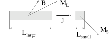
FIG. 1.: Model experimental setup. Current $j$ is passed through the nanowire with two magnetic pieces (shaded areas) with magnetizations ${\bf M}_{L}$ and ${\bf M}_{S}$. External magnetic field $\bf B$ can be applied in an arbitrary direction.

However for a real material one must also take into account magnetocrystalline and shape anisotropy. In this paper we present the first exact solutions with anisotropies taken into account. Attempts to incorporate them were made in the experimental reports [3, 4] and an extensive treatment of a particular experimental situation was given in a numerical study [10].

If the size of the pieces is larger then the domain wall width, the magnetization may be not uniform throughout the piece. In this case equations from [9] must be used inside each piece to determine the magnetic configuration. In this work we will assume that magnetic pieces are sufficiently small and treat them as magnetically uniform. Then the total anisotropy, including magnetocrystalline and shape contributions, will be given by a symmetric tensor $K^{(tot)}_{ik}$.

The problem simplifies if one of the magnetic pieces is much longer then the other. At a given current density $j$ the spin-transfer torque $T_{st}$ is proportional to the cross-section of the piece while the torques $T_{a}$ due to anisotropy are proportional to its volume. The ratio $T_{st}/T_{a}\sim 1/L$, where $L$ is the length of the piece, thus the small piece will be affected by the spin-transfer torque starting from a much smaller value of $j$. We can therefore neglect the effect of $T_{st}$ on the large piece, called a polarizer, and assume its magnetization to be constant. Magnetizations of the large and small pieces will be denoted as ${\bf M}_{L}$ and ${\bf M}_{S}$ respectively.

To test the theory, one would like to be able to control the direction of the magnetization of the polarizer with respect to the anisotropy directions of the small piece. The easiest way to change ${\bf M}_{L}$ is an application of an external magnetic field $\bf B$. Of course, $\bf B$ will also act on the small piece and must be taken into account in the equations of motion. The properties of a system with a given anisotropy $K_{ik}$ can ultimately be presented as a phase diagram in the $(j,{\bf B})$ space with spin-transfer effects determined by the magnitude of the current and by ${\bf M}_{L}={\bf M}_{L}({\bf B})$. In this paper we calculate a section of such diagram for certain directions of $\bf B$ and anisotropies. Note, that for technical applications in the memory writing process one is interested in finding anisotropy tensors which satisfy two conditions: (a) there is a section of the phase diagram at a fixed external field ${\bf B}={\bf B}_{0}$ where ${\bf M}_{S}$ is bistable at $j=0$; (b) by passing a current $j\neq 0$ one can switch between these two metastable states. However for the purposes of testing the theory it is better to start with the cases where the phase diagram can be calculated exactly and compare theoretical and experimental results.

In [10] stability of the zero-current equilibrium position of ${\bf M}_{S}$ was studied by an approximate analytical method and by numerical solution of a differential equation for the time evolution of ${\bf M}_{S}$. The latter gave the final position of magnetization and the details of the switching process. Due to the approximation used, there was a discrepancy between the switching thresholds predicted by two methods. In our study we find the equilibrium positions of ${\bf M}_{S}$ for each $(j,{\bf B})$ point and analyze their stability exactly. Knowing the nature of all equilibria we are able to construct the topology of the time-evolution flow of ${\bf M}_{S}$ and predict qualitatively the overall behavior of the system, including existence of the stable cycles. Such stable cycles were predicted in [13] and observed numerically in [10]. Due to energy dissipation they would be impossible without the current. However for $j\neq 0$ there is a constant supply of energy which feeds the periodic motion of ${\bf M}_{S}$.

Dynamic Equation for the Small Piece The magnetic energy of the small piece is a sum of the intrinsic anisotropy term, shape anisotropy term, interaction with external magnetic field and exchange interaction with the large piece. Approximating the shape of a monodomain small piece by an ellipsoid we can write

$$\frac{F}{V} = \frac{1}{2}\left(-K^{(intr)}_{ik}n_{i}n_{k}+4\pi M_{i}N_{ik}M_{k}\right)-B_{i}M_{i}-J_{ex}s_{i}n_{i}$$ (1)

where $N_{ik}$ is the demagnetization tensor [11], $M_{i}=M_{Si}$ - magnetization of the small piece, $K^{(intr)}$ - magnetocrystalline anisotropy tensor, and $J_{ex}$ is the exchange coupling between the pieces. Vectors ${\bf n}$ and ${\bf s}$ are unit vectors along the magnetization of the small and large pieces respectively. According to [7], the modified Landau-Lifshitz equation for ${\bf M}$ has the form:

$${\dot{\bf M}} = -\frac{\gamma}{V}{\dot{\bf L}}=\gamma[-\frac{\delta F}{\delta{\bf M}},{\bf M}]+$$ (2)

$$+ \frac{\gamma}{V}\frac{\hbar}{2}A\frac{j}{e}g(P,{\bf s\cdot n})[{\bf n},[{\bf s},{\bf n}]]+\tilde{\alpha}[{\bf n},\dot{\bf n}]$$ (3)

where $\gamma=g\mu_{B}/\hbar$ is the gyromagnetic ratio, $V$ and $A$ are the volume and cross-section area of the piece, the last term represents Gilbert damping, $P$ is the degree of spin-polarization of the electrons coming out of the large piece and $g(P,{\bf s\cdot n})$ is the function derived in [7]

$$g(P,{\bf s\cdot n}) = \frac{1}{f(P)(3+{\bf s\cdot n})-4},\;\;\;\;f(P)=\frac{(1+P)^{3}}{4P^{3/2}}$$ (4)

Equation (2) can be rewritten in terms of $\bf n$

$$\dot{n}_{i} = [{\bf h},{\bf n}]_{i}+K_{ik}n_{k}+Ig(P,{\bf s\cdot n})][{\bf n},[{\bf s},{\bf n}]]_{i}+\alpha[{\bf n},\dot{\bf n}]$$ (5)

with rescaled coefficients

$$h_{i} = \gamma(B_{i}+\frac{J_{ex}}{M}s_{i}),\;\;\;K_{ij}=\frac{\gamma}{M}(K^{(intr)}_{ij}-4\pi M^{2}N_{ij})$$ (6)

$$I = \frac{\gamma}{V}\frac{\hbar}{2}A\frac{j}{e}\frac{1}{M},\;\;\;\;\;\;\;\;\;\alpha=\frac{\tilde{\alpha}}{M}$$ (7)

The behavior of the small piece will be completely determined by the directions of $\bf s$ and $\bf h$ with respect to the principal axis of the anisotropy tensor $\hat{K}$. Dependence ${\bf s}={\bf s}({\bf h})$ is given by the properties of the polarizer. We will assume that the damping is small and expand the solutions in $\alpha$.

It was found recently [12] that cobalt nanowires grow with intrinsic easy axis perpendicular to the wire for large wire diameters $d\geq 50{\rm nm}$ and with easy axis along the wire for smaller $d$. As for the shape anisotropy contribution, it will be an easy axis along the wire if the length of the small piece $L_{S}>>d$ and an easy plane perpendicular to the wire in the opposite case $L_{S}<<d$. In [3, 10] a wire with $d\approx$ 100 nm was used. This complicates the situation because for any $L_{S}$ all three principal components of the total anisotropy tensor are different. On the contrary, for $d<50$nm wires anisotropy is always uniaxial. For $L_{S}>>d$ it is an easy axis along the wire. For $L_{S}<<d$ the total constant is given by $K=K^{(intr)}-4\pi M^{2}$. If $M$ is sufficiently large to ensure $K<0$, one has an easy plane anisotropy. This is the case for cobalt $K=5\cdot 10^{6}{\rm erg/sm}^{3}$ and $M=1.4\cdot 10^{3}{\rm emu}$.

We are going to consider two experimental situations with thin wires.

Axial Case. Assume that the polarizer is characterized by an easy axis anisotropy along the wire. The small piece has uniaxial anisotropy with respect to the same axis, but the anisotropy constant $K$ can have either sign. Next, assume that the external magnetic field is also directed along the wire which itself is oriented along the $z$-direction. Such situation with $K>0$ was considered before in [13] using a different method.

First we rewrite vector equation (5) in terms of the polar angles of ${\bf n}$: $\phi$ and $\theta$. That gives a system:

$$\left[\begin{array}[]{cc}\sin\theta&-\alpha\\ -\alpha\sin\theta&-1\end{array}\right]\left\{\begin{array}[]{c}\dot{\phi}\\ \dot{\theta}\end{array}\right\}=\left\{\begin{array}[]{c}v_{\phi}(\phi,\theta)\\ v_{\theta}(\phi,\theta)\end{array}\right\}$$ (8)

To find equilibrium positions one must solve

$$\left\{\begin{array}[]{l}v_{\phi}=\sin\theta(h+K\cos\theta)=0\\ v_{\theta}=Ig(P,\cos\theta)\sin\theta=0\end{array}\right.$$ (9)

When $I\neq 0$ the only stable positions of $\bf n$ on the unit sphere are the North and South poles, independent of the magnitude of current.

To determine the stability of equilibria we linearize the r.h.s. of (8) in small deviations. At $\theta=(0,\pi)$ one has to use local non-singular coordinates $x=\theta\cos\phi,y=\theta\sin\phi$. Linearized equations have the form

$$\left\{\begin{array}[]{c}\dot{\delta x}\\ \dot{\delta y}\end{array}\right\}={\hat{D}}\left\{\begin{array}[]{c}\delta x\\ \delta y\end{array}\right\}$$ (10)

The nature of equilibria is determined by the eigenvalues $\mu$ of the dynamic matrix $\hat{D}$. Real $\mu$’s imply a center or a saddle, while for complex-conjugate eigenvalues the stationary point is a stable focus for ${\rm Re}\mu<0$ or an unstable one otherwise.

Without showing the algebra we write down the result. For the North pole

$$\mu_{N}=-Ig(P,1)-\alpha(h+K)\pm i|h+K-\alpha Ig(P,1)|$$ (11)

and therefore it is a stable equilibrium for

$$j>-\frac{\alpha(h+K)}{g(P,1)}$$ (12)

For the South pole we get a stability criteria

$$j<-\frac{\alpha(h-K)}{g(P,-1)}$$ (13)

The regions of stability of the North and Sough poles are shown on Fig.2. It is important that there is a region on the diagram where both equilibrium points are unstable. This necessarily means that there exists a stable cycle, around which $\bf n$ performs a periodic motion.

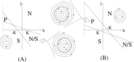
FIG. 2.: Switching phase diagram for the axial case. (A) easy axis in the small piece; (B) easy plane in the small piece. The left boundary (vertical dashed line) represents the switching field of the polarizer. Regions are marked as: N – only North pole is stable, S – only South pole is stable, N/S – bistable region, P – precession region. Time-evolution flow on the projected sphere (in which N is mapped to infinity and S to the origin) is shown on the insets.

In general, stability analysis can not give any information about the shape of the cycle, but in the axial case it is easy to anticipate that it will be given by $\theta=\theta_{0}$. From (8) the value of $\theta_{0}$ is given by $Ig(P,\cos\theta_{0})+\alpha(h+K\cos\theta_{0})=0$ and the precession frequency by $\omega=\left|Ig(P,\cos\theta_{0})/\alpha\right|$. When $h$ is decreased through the precession region at fixed current, $\theta_{0}$ changes continuously between $0$ and $\pi$ and $\omega$ increases from $\omega_{N}=|Ig(P,1)/\alpha|$ to $\omega_{S}=|Ig(P,-1)/\alpha|$. For the $K>0$ case $I\geq 2\alpha K/(g(P,-1)-g(P,1))$ in the precession region and the frequency has a minimal value $2Kg(P,1)/(g(P,-1)-g(P,1))$ of the order of FM resonance gap. For $K<0$ the frequency can go down to zero since there are $I=0$ points in the precession region.

Planar Case. We now consider a situation when the polarizer is characterized by an easy-plane anisotropy. The small piece has no choice but to have $K<0$ too, since by definition $L_{S}<<L_{L}$ and shape anisotropy must be even more important for it. In this experiment we direct the magnetic field perpendicular to the wire. As a result, we always have $\bf s$ along $\bf h$ and there is no meaning to negative values of $h$. We choose $s$ and $h$ to point in the $x$-direction.

Functions $v_{\phi}$ and $v_{\theta}$ for the planar case differ from the axial one. Working out their form we get a system of equations for the equilibrium points.

$$\left\{\begin{array}[]{l}v_{\phi}=K\cos\theta\sin\theta-h\cos\theta\cos\phi-Ig\cdot\sin\phi=0\\ v_{\theta}=h\sin\phi-Ig\cdot\cos\theta\cos\phi=0\end{array}\right.$$

where $g=g(P,\sin\theta\cos\phi)$. It is that dependence of $g$ on both $\theta$ and $\phi$ that brings the main complication into the solution for the planar case.

Both equations are satisfied for $\cos\theta=\sin\phi=0$. Consequently there is a pair of equilibria: point $A$ $(\phi=0,\theta=\pi/2)$ and point $B$ $(\phi=\pi,\theta=\pi/2)$, positions of which do not depend on the current magnitude. There are however additional equilibria given by

$$\left\{\begin{array}[]{l}K\sin\theta-\cos\phi(h^{2}+I^{2}g^{2})/h=0\\ h\sin\phi=Ig\cdot\cos\phi\cos\theta\end{array}\right.$$ (14)

To deal with the $\phi,\theta$ dependence of $g$ we make a variable change

$$\left\{\begin{array}[]{l}\cos\phi\sin\theta=x\\ \sin\phi=y\end{array}\right.$$ (15)

Then $g=g(P,x)$. It is an important property of the model and the planar case geometry, that this substitution succeeds in reducing system (14) to a relatively simple decoupled equation on $x$:

$$1+(\eta xg(P,x))^{2}=\frac{x}{x_{0}}$$ (16)

with $x_{0}=h/K<0$ and $\eta=I/h$.

Investigation of (16) shows that as $\eta$ increases, there will be one, two or zero roots. We will see below, that switching happens already at small currents, where only one root exists and where we can expand the solution as $x=x_{0}+\eta x_{1}+\ldots$. This root defines two symmetric equilibrium points $C_{1,2}$ located as shown on Fig.3 inset. Their positions depend on the magnetic field. As $h$ grows, both $C$ points move gradually towards $B$ and merge with it at $h=|K|$. At higher $\eta$ we observe additional roots - the full $(I-h)$ diagram will be published elsewhere.

Stability analysis shows, that point $A$ becomes unstable at a negative current with a magnitude $I_{\rm sw}\sim\alpha$, similar to the axial case. That justifies the expansion of $x$ above. As in the axial case, we only present the eigenvalues of the dynamic matrix at all equilibrium points.

For point $A$

$$\mu_{A}=-Ig(P,1)-\frac{\alpha(-K+2h)}{2}\pm i\sqrt{h(-K+h)}$$ (17)

Therefore $A$ is a focus point. Its stability is given by

$$I>-\alpha\frac{-K+2h}{2g(P,1)}$$ (18)

Linearization near point $B$ gives

$$\mu_{B}=Ig(P,-1)+\alpha\frac{2h+K}{2}\pm\sqrt{-h(h+K)}$$ (19)

Therefore point $B$ is a saddle point for $h<|K|$ and is a focus for greater field. In the latter case $B$ is stable if

$$I<-\alpha\frac{2h+K}{2g(P,-1)}$$ (20)

Treatment of both points $C_{i}$ gives identical results

$$\mu_{C} = \frac{1}{2}\left[Ig\cdot\left(\frac{1+\cos^{2}\theta}{\sin\theta}+\sin\theta-fg(P,x_{0})\;\cos^{2}\theta\right)-\right.$$ (22)

$$\left.2\alpha K+\alpha\frac{h^{2}}{K}\right]\pm i\sqrt{K^{2}-h^{2}+O(I)}$$

In the region of its existence ($h<|K|$) point $C$ is always a focus. The stability region is given by

$$I<-\alpha K\frac{x_{0}(2-x_{0}^{2})}{2+fg(P,x_{0})(1-x_{0})^{2}x_{0}}$$ (23)

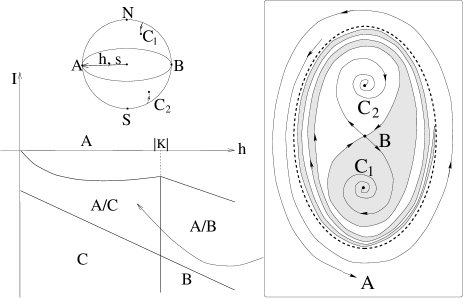
FIG. 3.: Switching phase diagrams for the planar case. Regions are marked by letters corresponding the stable points. Bistable regions are marked by A/C and A/B. Right: time-evolution flow on the projected sphere for bistable $A/C$ situation - basin of attraction for $C_{1}$ is shaded. Upper inset: stable points $A,B,C_{i}(I)$ on the unit sphere.

Inequalities (18,20,23) determine the switching phase diagram in the small $\alpha$ limit (Fig.3). In the planar case only bistable regions exist and there is no precession region on the phase diagram. We also note that the basins of attraction of $C_{1}$ and $C_{2}$ are increasingly interpenetrating near the boundary separating them from the basin of attraction of $A$ (Fig.3). In switching from $A$ to $C$ the choice between $C_{1}$ and $C_{2}$ is random.

Discussion. Switching patterns depend crucially on the magnetic anisotropy and the direction of polarization of incoming current. Our predictions for the axial and planar cases can be used to experimentally test the theory , in particular the accuracy of the factor $g(P,{\bf s\cdot n})$ [7]. This is especially interesting because alternative descriptions of current driven excitations are put forth in the literature [14, 15]. Since currently magnetization directions are not experimentally measured but rather inferred from the resistive state of the wire, it is important that there are qualitative differences between axial and planar cases. In the axial case all boundaries on the $(I-h)$ diagram are straight lines, while in the planar case one of them is curved. Current sweep through the precession region in the axial case will show three resistive states without hysteresis, while a sweep through the bistable region gives two jumps with a hysteresis. If ${\bf M}_{S}$ is measured directly, one will see that it rotates by $180^{0}$ degrees in the axial case and by a magnetic field dependent angle $\pi/2+\theta_{0}(h)$ in the planar case. The precession state is a good candidate for observation with a magnetic force microscope.

The switching current density can be calculated by substituting (6) into (12, 13) and (18,20,23). As a characteristic value one can take

$$I=\alpha\frac{|K|}{g(P,1)}\;\;\Rightarrow\;\;j=\alpha\left(\frac{e}{\hbar}\right)\frac{|K^{(intr)}-4\pi M^{2}|}{L_{S}}$$

For the size of the small piece $L_{S}=1{\rm nm}$, damping $\alpha=0.05$ and 40% polarization degree one gets $j\approx 6.7\cdot 10^{7}{\rm A/cm}^{2}$ using the values of $K^{(intr)}$ and $M$ for cobalt.

It is our pleasure to thank J.Z.Sun, J.Slonczewski and S.P.P.Parkin for stimulating discussions. Y.B.B. acknowledges support from David and Lucile Packard Foundation Fellowship in Science and Engineering, B.A.J. thanks the Aspen Center for Physics for hospitality, S.C.Z. was supported by NSF grant DMR-9814289.

REFERENCES

- [1] M.Tsoi et al., PRL 80, 4281 (1998)
- [2] J.E.Wegrowe et al., Europhys.Lett. 45, 626 (1999)
- [3] E.B.Myers et al., Science 285, 867 (1999); J.A.Katine et al., PRL 84, 3149 (2000)
- [4] J.Z.Sun J.Magn.Magn.Mater. 202, 157 (1999)
- [5] J.Slonczewski, US Patent # 5,695,864. Dec,9, 1997;
- [6] Collection of articles in IBM J. Res. Dev. 42 (1998)
- [7] J.Slonczewski, J.Magn.Magn.Mater. 159, L1 (1996)
- [8] L.Berger PRB 54, 9353 (1996), J.Appl.Phys. 81, 4880 (1997)
- [9] Ya.B.Bazaliy et al., PRB 57, R3213 (1998)
- [10] J.Z.Sun, PRB 62, 570 (2000)
- [11] L.D.Landau, E.M.Lifshitz, Electrodynamics of Continuous Media, sec.45, Reed Elsevier, 1996
- [12] J.L.Maurice et.al. J.Magn.Magn.Mater.184, 1, 1998; Y.Henry et al., to be published; U.Ebels et al., PRL 84, 983, 2000
- [13] J.Slonczewski, unpublished talks on many conferences, including APS 2000, EMMA2000, IBM talks etc.
- [14] L.Berger, preprint (2000)
- [15] X.Waintal et al., cond-mat/0005251 (June,2000)