Abstract

The problem of two electrons in a two-dimensional random potential is addressed numerically. Specifically, the role of the Coulomb interaction between electrons on localization is investigated by writing the Hamiltonian on a localized basis and diagonalizing it exactly. The result of that procedure is discussed in terms of level statistics, the expectation value of the electron-electron separation, and a configuration-space inverse participation number. We argue that, in the interacting problem, a localization-delocalization crossover in real space does not correspond exactly to a Poisson-Wigner crossover in level statistics.

PACS 71.23An; 71.30$+$h; 71.23$-$k

§1. Introduction. The problem of two interacting particles (TIP) in a random potential has received much attention in the last few years. The focus has been primarily on TIP in one dimension (1D), where most investigators have dealt with particles interacting via an on-site potential. (For a concise summary of the various approaches used, and results obtained, we refer the reader to the articles in ref. [1].) The reason for all the attention (and controversy) is the result, first found by Shepelyansky [2], that the TIP actually propagate coherently through a length much larger than the one-particle localization radius, which can lead to an enhancement of transport [3]. We address the related problem of localization in 2D systems, and how it is affected by a long-range electron-electron interaction (EEI).

The more general problem of the interplay between disorder, interaction and quantum tunneling, and their combined effect on electronic localization is not new. While the Hartree Coulomb repulsion introduces an additional random energy and thus enhances localization, the possibility that quantum correlation due to the EEI may act to delocalize the electrons was proposed twenty years ago by Pollak and Knotek [4], and Pollak [5], but a firm answer has not been achieved yet. Computationally, the main difficulty in the finite-electron-density problem is the huge phase space for systems of reasonable size [6]. Existing work [6, 7, 8, 9, 10] resorted to various approximations. In contrast, the TIP problem for reasonably large systems can be solved without such approximations: double occupation of sites can be accounted for, spin and exchange included, and the entire phase space can be examined. A motivation for the problem considered here is the ability to make inferences about approximations made in investigations of finite-density and few-electron systems [11, 12, 13, 14, 15, 16]. We hope furthermore that the work may contribute to insight into the mechanisms at play in the experimental reports on an observed metal-insulator transition (MIT) in 2D [17].

In the present paper, we deal with two electrons in a random potential interacting via a long-range Coulomb interaction, and investigate numerically the effect of that EEI on electronic localization. A tool used frequently to assess localization has been the distribution $p(s)$ of nearest-level spacings $s$. In the absence of interactions, it has been shown [18] that $p(s)$ shifts from Poisson to Wigner as the system goes from being strongly localized to delocalized. (The salient difference between the two distributions is that Poisson is maximal as $s\rightarrow 0$, while Wigner vanishes there.) For interacting systems, such correspondence has never been proven. Still, level spacing statistics has been used often to study localization also with interactions. This may be reasonable because interaction is not relevant to the logical connections between the localization $\leftrightarrow$ delocalization and Poisson $\leftrightarrow$ Wigner transitions: off-diagonal energies cause hybridization of site functions and thus delocalization, while at the same time they increase level repulsion and thus eliminate small level spacings. This is not to say that the same criteria for the Anderson transition that were established for non-interacting systems can be automatically taken over for interacting systems. An interesting case in point is a study of the Two-Body Random Interaction Model (TBRIM). Georgeot and Shepelyansky [19] found that in that model a huge number of non-interacting eigenstates contribute to the interacting eigenstates (indicating possible delocalization in real space) even in situations when $p(s)$ is close to Poisson. On the other hand, Jacquod and Shepelyansky [20] used, for the same model, the Wigner-Poisson transition to establish a transition from integrability to chaos.

A quantity used commonly to study delocalization in non-interacting systems is the inverse participation number $P^{-1}$ [21], which measures over how many sites the (one-particle) wavefunction spreads. Here, where we allow for interactions, we use an analogous quantity, the configuration-space inverse participation number $R$ (see ref. [22] and eq. (6) below) which measures over how many configurations the many-particle wavefunction spreads. In the limits of strong localization and of complete delocalization it is easy to see the connection between $P^{-1}$ and $R$: the strong-localization limit, $R=1$, implies the presence of a single configuration, which in turn implies that each particle is localized on a single site. In the complete delocalization limit, $R=1/\tilde{N}$ (where $\tilde{N}$ is the total number of configurations), the wavefunction extends uniformly over all configurations, implying that the particles are uniformly spread over the system in real space.

Previous studies on 2D random systems with interactions most relevant to this work include finite-size scaling of three and four [11], and two [12, 13, 14, 15, 16] spinless electrons. All these works have concluded that the interaction enhances delocalization. In [11] a crossover from Poisson to Wigner was found, while [12, 13, 15] reported a sharp transition with an identifiable critical point. We shall see that the enhanced accuracy of this study does not alter the conclusion that interaction enhances delocalization through most of the energy domain.

In the next two sections, we explain the details of our approach, and describe the difference with other authors’ methods. In the fourth section, we present our results, and then we offer in the conclusion some final remarks.

§2. The Model. In the standard approach (see, e.g. refs. [11, 15]) to the problem at hand (sometimes referred to as the Quantum Coulomb Glass [9]), one considers spinless electrons on sites of a lattice and represents the Hamiltonian in the basis of local wavefunctions:

$$H_{QCG}=t\sum_{\{ij\}}(a_{i}^{\dagger}a_{j}+h.c.)+\sum_{i}\epsilon_{i}a_{i}^{\dagger}a_{i}+U\sum_{i>j}(a_{i}^{\dagger}a_{i}a_{j}^{\dagger}a_{j}+a_{i}^{\dagger}a_{j}a_{j}^{\dagger}a_{i})/|\vec{r}_{i}-\vec{r}_{j}|$$ (1)

where $\{ij\}$ denotes nearest-neighbor (n-n) sites, the operator $a_{i}^{\dagger}$ ($a_{i}$) creates (destroys) a (spinless) electron at site $i$; $\epsilon_{i}$ is a random site energy chosen in the range $-W/2<\epsilon_{i}<W/2$ with uniform probability; $U$ is the strength of the Coulomb interaction; $\vec{r}$ is a position vector. Both $U$ and $W$ are taken as independent parameters.

Our model differs primarily in that we include spin, and treat more extensively the overlaps. The latter is done in two ways: we do not neglect fluctuations in the n-n overlap integrals (due to the differing charge environments at different pairs of sites), and include overlaps over other than just nearest-neighbors (as we cross the MIT from the insulating side, the increase in the number of important distant sites may be more decisive than the decrease in the n-n overlap.)

To accomplish the above we write the two-electron wavefunctions in terms of a basis set of appropriately symmetrized products of the one-particle local wavefunctions

$$\Phi_{ij} = \phi_{ij}^{(S)}\times\sigma^{(A)}\mathrm{,and}$$ (2)

$$\Phi_{ij} = \phi_{ij}^{(A)}\times\sigma^{(S)}\mathrm{,}$$ (3)

where $i,j$ are site labels, $\phi_{ij}$ ($\sigma$) is the spatial (spin) part of the two-electron configuration, and the superscripts $S$ and $A$ indicate the symmetry of the wavefunction under particle exchange. The $\phi_{ij}$ are constructed in the usual manner, i.e. by symmetrizing (or antisymmetrizing) products such as $\varphi_{i}(1)\varphi_{j}(2)$ of one-electron orbitals (centered on $i$ and $j$) $\varphi$ for electrons 1 and 2. Double occupation of sites comes in through $\phi_{ii}^{(S)}$. Clearly, the $\phi_{ij}^{(S)}$ ($\phi_{ij}^{(A)}$) are singlet (triplet) configurations. We take $\varphi\sim\exp(-r/a_{B})$, with $r$ the electron-core distance and $a_{B}$ the microscopic (Bohr) radius corresponding to those orbitals.

We write the Hamiltonian

$$H = \sum_{\alpha=1}^{2}(T_{\alpha}+V_{\alpha}+\varepsilon_{\alpha})+\frac{e^{2}}{\kappa r_{12}},\mathrm{with}$$ (4)

$$T_{\alpha} = -\frac{\hbar^{2}}{2m^{*}}\nabla^{2}_{\alpha},$$

$$V_{\alpha} = -e\cdot q_{s}\sum_{i=1}^{n_{s}}\frac{1}{\kappa r_{i\alpha}}\mathrm{,and}$$

$$\varepsilon_{\alpha} = \sum_{i=1}^{n_{s}}\epsilon_{i}\delta(\vec{r}_{\alpha}-\vec{r}_{i}),$$

where $\alpha$ labels the electrons, $T$, $V$, and $\varepsilon$ are the operators corresponding to the kinetic energy, the interaction of the electrons with the cores, and the random potential, respectively; $e$ is the electronic charge; $\kappa$ is the dielectric constant; $r_{12}$ is the electron-electron (e-e) distance; $m^{*}$ is the electron mass; $q_{s}$ is the charge on a site; $n_{s}$ is the number of sites in the system; $\epsilon_{i}$ is a random energy chosen as in eq. (1), with $W$ equal to the n-n Coulomb energy $e_{C}$ (i.e. we set $W=U=1$ in units of a n-n Coulomb energy). We vary the site concentration by changing the n-n distance $r_{nn}$ as a parameter.

Analytic solutions for $\langle\phi_{ij}^{(S)}|H|\phi_{kl}^{(S)}\rangle$ and $\langle\phi_{ij}^{(A)}|H|\phi_{kl}^{(A)}\rangle$ were derived and written in terms of one-, two-, three-, and four-center integrals. The procedure is very tedious but straightforward. The equations are not given here for reason of space, and because the TIP case is not general; the equivalent expressions for systems with an arbitrary number of spinless fermions were published in [22]. The integrals were performed numerically for processes $\{ij\}\rightarrow\{kl\}$ which involved (i) no electron transfers (i.e. diagonal matrix elements); or (ii) a one-electron n-n transfer; or (iii) a next n-n transfer; or (iv) a next-to-next n-n transfer; or (v) two simultaneous n-n transfers. All other off-diagonal matrix elements were set to zero. $H$ does not depend on spin, so $\sigma$ enters into the picture only by dictating the symmetry (under particle exchange) of the corresponding $\phi_{ij}$. Naturally, the off-diagonal matrix elements between $\phi_{ij}$ of different symmetry are set to zero; thus the matrix $H$ splits into two blocks which we diagonalize separately using standard techniques. The result is the set of eigenenergies $E_{I}$, and the corresponding states $\Phi_{I}$ in which the $\phi_{ij}$ come in with amplitudes $A_{I,ij}$:

$$\Phi_{I}^{(S)}=\sum_{\{ij\}}A_{I,ij}^{(S)}\phi_{ij}^{(S)},\textrm{ and }\Phi_{I}^{(A)}=\sum_{\{ij\}}A_{I,ij}^{(A)}\phi_{ij}^{(A)}.$$ (5)

For simplicity we refer below to $\Phi_{I}^{(S)}$ as “singlets” and $\Phi_{I}^{(A)}$ as “triplets”.

In this work we take $W$ to always equal $e_{C}$; thus, $W=e_{C}\sim 1/r_{nn}$. Since $r_{nn}$ is a parameter here, $W$ changes accordingly. We do this because then the effect of interaction is most important, and also because this condition prevails in many experiments, for example, in the vast experimental literature on impurity conduction at moderate compensation [23]. In impurity conduction $W$ corresponds to the Coulomb energy over the mean n-n majority-minority ion distance, while $U$ corresponds to the Coulomb energy over the mean carrier-carrier separation. The two are quite similar unless the compensation is either very small or very large.

The present model also differs from other models in how it deals with electrical neutrality. In most works neutrality is achieved by placing a compensating charge $q_{s}=+|e|n_{e}/n_{s}$ on every site. However, since the microscopic radius of the electrons is usually determined by the charge $q_{s}$ of the core, this radius would strongly depend on how electrical neutrality is established. (For the TIP problem $n_{e}$ is fixed, but $n_{s}$ is generally taken as a parameter; thus, different models for compensation may in fact yield different results.) To avoid such problems, this work does not consider the compensating charge explicitly. To make contact with experimental situations, we place a core charge of magnitude $+|e|$ at each site. The macroscopic radius is then determined by an effective mass and a dielectric constant. Since there are more sites than carriers, the system is not neutral. A question we need to answer is whether the properties of interest here, i.e. the degree of localization and its dependence on various parameters, are fundamentally affected by the lack of neutrality. To answer this question we consider whether one can construct some model for the compensating charge such that it has no effect on the results of the computations as far as the localization properties are concerned. The answer is that such a model exists, namely a spatially uniform distribution of the compensating charge (which may be placed on a separate plane, not unlike the situation in gated devices). This charge merely contributes two constant energies: a self-interaction, and the interaction with the two electrons. We may thus conclude that the lack of neutrality per se does not affect our results. However, it should be borne in mind that in reality the particular way in which charge neutrality is realized may affect somewhat the localization properties.

§3. Procedure. We set up “samples” on the computer with $n_{s}$ ($=L\times L$) sites arranged on a lattice, and diagonalize eq. (4) for the parameters $L$ and $r_{nn}$. For definiteness, we take $a_{B}$ and $\kappa$ to be 10Å and 3 respectively, which yields and effective mass $m^{*}=0.16m$, with $m$ the electron mass – these values seem appropriate for 2D systems. Cyclic boundary conditions are used. In what follows, we use $a_{B}$ as the unit of distance. In every case the number of samples was sufficient to obtain at least $1.5\times 10^{4}$ levels for each pair $\{n_{s},r_{nn}\}$.

As one measure of localization, we compute $p(s)$. (We dropped up to 100 states from the band edges.) As in [12], a parameter $\eta=(\mathrm{var}(s)-0.273)/(1.0-0.273)$ is computed as a measure of how close $p(s)$ is to a Poisson ($\eta=1$) or Wigner ($\eta=0$) distribution. As an alternate measure of localization we compute the configuration-space inverse participation number as in ref. [22]:

$$R_{I}=\sum_{\{ij\}}|A_{I,ij}|^{4}.$$ (6)

In addition to $p(s)$ and $R_{I}$ we examine the behavior of the quantity

$$\lambda_{I}=\sum_{\{ij\}}r_{ij}|A_{I,ij}|^{2},$$ (7)

which is the expectation value of the e-e separation when the system is in state $\Phi_{I}$. This expectation value is computed here for a direct glimpse at the behavior of the $\Phi_{I}$ in real space. One expects that in the localized regime $\lambda_{I}$ is strongly correlated with $E_{I}$ due to the EEI (larger $\lambda_{I}$ correspond to smaller $E_{I}$), whereas $\lambda_{I}$ should become essentially independent of $E_{I}$ as configuration-mixing increases. In the absence of interactions, such correlations should of course not be present.

To measure the importance of secondary tunneling processes, we investigate the following quantities: (i) the width $w$, and the average $t_{nn}$ of the distribution of off-diagonal elements corresponding to n-n processes; (ii) the sum $S^{(1)}$ of all off-diagonal elements corresponding to n-n processes; (iii) a similar sum $S^{(\sqrt{2})}$ for all next n-n processes; and (iv) a sum $S^{(2)}$ of such matrix elements which correspond to either next-to-next n-n or two simultaneous one-electron n-n transfers. We note that the sums $S^{(\cdots)}$ account in a crude way for not only the magnitude of the off-diagonal matrix elements, but also for the size of the phase space occupied by those processes (e.g. even though a matrix element corresponding to a n-n transition may be significantly larger than one corresponding to two simultaneous n-n transfers, the number of matrix elements of the latter type is much larger – and thus such processes may contribute significantly to coherent tunneling). Also, we note that the standard approach assumes $t_{nn}\gg w$, $S^{(1)}\gg S^{(\sqrt{2})}$ and $S^{(1)}\gg S^{(2)}$.

§4. Results and discussion. Double occupation of sites does not, of course, occur in the triplets case, and a single band of eigenenergies results from the diagonalization procedure. The width of this band naturally increases with decreasing $r_{nn}$ because the configurations hybridize, and level repulsion increases. For singlets, however, at large $r_{nn}$ two such bands separated by a gap result: a lower band arises from hybridization of configurations in which sites are singly occupied (to which we will refer as type-s configurations) – as in the triplets case, and an upper band arises from configurations in which sites are doubly-occupied (type-d configurations), which for the most part do not hybridize; with decreasing $r_{nn}$, the gap narrows as (mostly type-s) configurations hybridize, and level repulsion increases. As $r_{nn}$ is decreased further, type-d configurations start to mix with each other, and with type-s configurations, until eventually (for $r_{nn}\leq\sim 4$), the gap actually disappears, and the two bands start to join together. We present results here for $r_{nn}=4\textrm{-}12$. In what follows, except for our discussion of $\lambda_{I}$, our results refer to the triplets band, and to the singlets’ lower band.

We first present the basic conclusions regarding the effect of the EEI on localization. Fig. 1 shows a comparison of $\eta(r_{nn})$ between the interacting and non-interacting systems [i.e. eq. (4) without the last term]. It is very clear that this criterion shows EEI to enhance delocalization – while with EEI delocalization occurs at $r_{nn}\sim 10$, without EEI delocalization is out of the range of the figure, namely somewhere at $r_{nn}<7$. We note that there is no clear small-size scaling behavior, suggesting a crossover ($r_{nn}\sim 9\textrm{-}11$), rather than a critical transition. This is in agreement with [11], but differs from [12, 13, 15, 16]. The differences may be due to differences in models and choice of parameters [24].

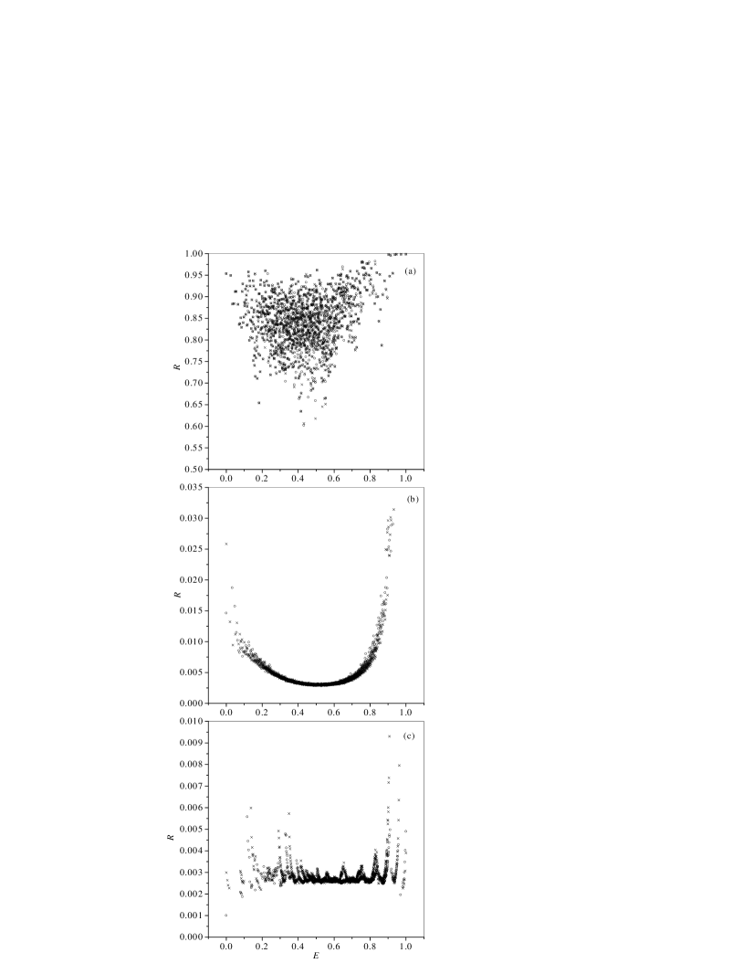
Figure 2: Inverse participation number in configuration space $R$ with $L=7$ for singlets ($\circ$) and triplets ($\times$), and (a) $r_{nn}=12$; (b) $r_{nn}=8$; (c) $r_{nn}=6$. The energy scale is described in the text.

We present in figs. 2 and 3 our results for $R_{I}$ with $L=7$, but we checked that the plots for other values of $L$ are qualitatively the same. To evaluate the importance of spin, we plot in fig. 2 the number $R_{I}$ for singlets and triplets. In both cases, the energies are measured from the bottom of the band, and have been normalized by the energy difference between the top and the bottom of the band. The most noticeable features in fig. 2 are: 1) in the localized regime [fig. 2(a)] there is no discernible difference between singlets and triplets; 2) For $r_{nn}$ close to the transition and into the delocalized regime, the lowest energy states of the singlets are always more delocalized than the lowest energy triplets. This is exemplified by figs. 2(b) and 2(c). This difference between the singlets and the triplets seems to be larger the smaller the $r_{nn}$. 3) In the well-delocalized regime there appear intriguing fluctuations of $R_{I}$ with energy, for both singlets and triplets, as exemplified by fig. 2(c). The fluctuations are not random – there is a definite correlation in $R_{I}$ over a finite distance in energy. This persists from one realization of random energies to another, and persists also for increased $L$, though with a different characteristic correlation width. Possibly the fluctuations are connected with interference effects that come into play, due to our use of cyclic boundary conditions, once the extent of the wavefunction spans the entire system. Interestingly, similar fluctuations were observed [25] in a real-space inverse participation ratio for TIP in the Harper model where the non-interacting eigenstates are delocalized.

In fig 3, $\rho$ is the average (over singlets and triplets) $R_{I}$ with EEI to the average $R_{I}$ without the interactions, i.e. $R_{I}$ is computed with and without the last term in eq. (4), and the results are averaged over singlets and triplets – $\rho$ is given by the ratio of the two averages. Thus, $\rho<1$ indicates delocalization (in configuration space) induced by the EEI, whereas $\rho>1$ points to interaction-induced localization. Over most of the regime of $E_{I}$ the plots confirm the previous result about the effect of EEI on delocalization. However, at the extremes of the energy regime, the opposite appears to happen – the wavefunctions for the interacting system are more localized, at least in configuration space. (It has been shown [26] that EEI can, under certain conditions enhance either localization or delocalization, and this in fact has been found to be the case [10].) We discuss the enhanced localization at the band edges in the context of [26]. The enhancement or supression of localization depends on the general effect of the EEI on the ratios $H_{IJ}/D_{IJ}$, where $H_{IJ}\equiv\langle\Phi_{I}|H|\Phi_{J}\rangle$ and $D_{IJ}\equiv\langle\Phi_{I}|H|\Phi_{I}\rangle-\langle\Phi_{J}|H|\Phi_{J}\rangle$. [Configuration indices $I$, $J$ here replace the pair indices $i$, $j$ of eqns. (2) and (3).] If the EEI enhances $H_{IJ}/D_{IJ}$ it supresses localization, in the opposite case it enhances it. $H_{IJ}$ and $D_{IJ}$ are both separately enhanced by the EEI [26], so the effect on localization depends on which is enhanced more. Now consider, for example, the lower band edge, i.e. the very low-energy end of the spectrum. The level spacing, and thus $D_{IJ}$, is enhanced by the interaction because it excludes configurations with nearby electrons. The enhancement of $H_{IJ}$ by interactions comes to a large degree from correlated n-particle (here 2-particle) transitions, but this effect is important mainly when the electrons are reasonably close-by. A somewhat parallel argument can be made for the upper band edge. It is interesting to note that similar effects of enhanced localization were reported in [25] for rather different systems.

We consider next the question of e-e separation due to interaction as measured by $\lambda_{I}$. Without the EEI the positions of the two electrons are uncorrelated so $\lambda_{I}$ is expected to vary at random from configuration to configuration and we ascertained that this is indeed the case. Fig. 4 shows polynomial fits for $\lambda_{I}(E_{I})$ with EEI for $L=7$. (Again, we checked that the results for other values of $L$ are qualitatively the same.) Fig. 4(a) corresponds to singlets, and fig. 4(b) to triplets. The numbers on the graph refer to the values of $r_{nn}$. In the singlets case we now include both bands. This figure is similar to results presented in [27], but here we present an average over many realizations of the random potential. In figs. 4(a) and (b) the energies are measured from the bottom of the lower band. In fig. 4(a) the energies are normalized to the energy difference between the top of the upper band the the bottom of the lower band; for comparisons between figs. 4(a) and (b), the triplets’ energies have been normalized so that the top of their band coincides with the top of the singlets’ lower band. The results shown in the figure can be conveniently discussed by dividing the plots into three groups: 1) The singlets [fig. 4(a)] include states at the high energy end of the figure which do not have a triplet counterpart [fig. 4(b)]. As discussed above, these states correspond to double occupation of sites: for large $r_{nn}$, $\lambda_{I}$ is quite small and the energy large, as expected for two electrons residing on the same site. As $r_{nn}$ decreases, some states still have the large energy, but now $\lambda_{I}$ is larger (as is evident from the steep lines with $r_{nn}=4,5$). These are likely to be states with a reasonably large component of a doubly-occupied site, hybridized with configurations where electrons are more remote from each other. The other features of fig. 4 are common to the triplets and the singlets and correspond to states where double occupation of sites is minimal or non-existent. 2) The curves representing large values of $r_{nn}$ (small overlaps) are quite steep, i.e. $\lambda_{I}$ decreases sharply with increasing $E_{I}$. This is easily understandable as an increase in the repulsion energy with a decreasing distance between occupied sites, i.e. decreasing $\lambda_{I}$. 3) The dependence of $\lambda_{I}$ on $E_{I}$ weakens as $r_{nn}$ decreases and configuration-mixing increases – $\lambda_{I}$ becomes nearly independent of $E_{I}$ and quite large for $r_{nn}=5$. The crossover takes place around $r_{nn}=6\textrm{-}9$ in both fig. 4(a) and (b).

We note that the crossover in $\lambda_{I}$ is lower than in fig. 1. In this model, $W/t=e^{r_{nn}}/[r_{nn}(1+r_{nn})]$, so a small difference in $r_{nn}$ implies a comparatively larger one in $W/t$. This gives $W/t\sim 3,5,10,20,40,90,200,500,1000$ for $r_{nn}=4,5,6,7,8,9,10,11,12$, respectively. One must be careful, however, when comparing our results with those of other authors because here $W/t=e_{C}/t$.

In fig. 5 we present our analysis of the importance of fluctuations in n-n hopping energies, and of secondary hopping processes. First we note that the relative width of the distribution of n-n hopping energies remains roughly constant with $r_{nn}$, and decreases with system size. As the size of the phase space increases with $n_{s}$, the relative importance of these fluctuations decreases, and probably disappears in the thermodynamic limit. Furthermore, secondary hopping processes are not very important in the localized regime; however, they are important (as expected) in the delocalized regime. These processes become significant for $r_{nn}\leq\sim 6$, and in fact, next-to-next n-n and simultaneous n-n processes are more important than next n-n in the delocalized regime. We surmise that these secondary processes “push” the transition towards higher values of $r_{nn}$.

We now turn to the specific aspects learned from those features of our model which go beyond other works [12, 13, 14, 15], namely the inclusion of spin and the more general consideration of elastic tunneling. We note that: 1) As expected, spin plays no role deep in the localized regime (since the exchange energy is proportional to $\langle\varphi_{i}|\varphi_{j}\rangle^{2}$). More unexpectedly, spin also seems to have little importance near the crossover to delocalization. Perhaps spin plays a larger role when one considers more than two electrons. 2) Type-d configurations play little or no role near the crossover – they become important only for $r_{nn}\leq\sim 4$. 3) In the localized extreme (i.e. $r_{nn}\geq 12$), the rather short span in energy of the eigenstates comes from the random and Coulomb energies; as $r_{nn}$ decreases, the broadening of the range of eigenenergies is attributable to the growing off-diagonal energies of $H$. 4) The standard model underestimates the delocalizing effect of the EEI for small $r_{nn}$ especially, as shown in fig. 5. Many-electron coherent processes are probably important in the finite-electron-density problem. This phenomenon was first pointed out in [8]. Secondary processes are important especially in the delocalized regime – one should consider them if investigating systems around the MIT.

§5. Conclusions. The model used here yields zero density in the thermodynamic limit, and so no definite claims or comparisons with experiments can be made. However, if we take the electronic localization-delocalization transition at $r_{nn}=6$, this simple model yields the critical concentration $n_{c}=10^{11}\textrm{ cm}^{-2}$. Whereas our systems are quite different from the experimental ones (see, e.g. [28], where a 2D MIT was reported for high-mobility systems at low temperatures), it is interesting to note that the experimental value of $n_{c}$ is the same as here. This of course might be just fortuitous.

Where collective hopping of the two electrons is coherent ($r_{s}\leq\sim 7$), $\lambda$ can be interpreted as a coherence length. It is of interest to note that a crossover of $p(s)$ from Poisson to Wigner occurs at a somewhat larger $r_{nn}$ than the crossover from a large variation in $\lambda_{I}(E_{I})$ to $\lambda_{I}(E_{I})\sim\mathrm{const.}$ We have included in our level spacing analysis most of the eigenstates of eq. (4), as opposed to only states in the middle of the band, which is the customary procedure (see e.g. [11, 12, 15]). Since we are including states which tend to be more localized than those in the middle of the band (as is evident from fig. 3), the effect is that our level spacing statistics picture is skewed towards the localized regime. The disagreement between the crossover on $p(s)$ and that in $\lambda_{I}$ would be stronger if we were to follow standard practice. We believe that (unlike in the non-interacting case) for interacting systems, delocalization in real space requires a somewhat larger overlap for n-n sites than does the transition to Wigner statistics. This is in keeping with previous work [22, 29], where it was observed that the wavefunctions are “swiss cheese-like” (i.e. not compact in real space) without EEI, but space-filling with the interactions [30]; therefore, while the EEI may make the wavefunction extend over more sites, it does not similarly increase its spatial extent – $\lambda_{I}$ might require a larger overlap than $p(s)$ (for a crossover to take place) because the EEI makes the wavefunction more compact in real space. In a sense, there is a similarity here with [19], where it was shown that interacting eigenstates may contain contributions from many non-interacting eigenstates, even when $p(s)$ is close to Poisson. The difference is that we get $p(s)$ close to Wigner in some situations when one might expect Poisson. For example, from fig. 4, at $r_{nn}=9$ one would expect $p(s)$ similar to Poisson since $\lambda_{I}$ depends strongly on $E_{I}$; however, fig. 1 reveals that $p(s)$ is nearly Wigner. We attribute the discrepancy between this work and the result in [19] to the different models used.

It is clear that $p(s)$ is Poisson well inside the localized regime, and Wigner well into the delocalized regime; however, the crossover in level statistics and its relationship to a localization-delocalization transition in real space is not as well established as it is in the non-interacting problem, and requires further study. Furthermore, whereas it is clear that deep localization in configuration space implies deep localization in real space, and the same holds true for well-delocalized systems, the actual transition need not occur simultaneously in the two domains.

Acknowledgements. The support of the National Science Foundation under grant DMR-9803686 is gratefully acknowledged, as are conversations with I. Varga, and some useful comments by the (unfortunately anonymous) second referee of this paper.

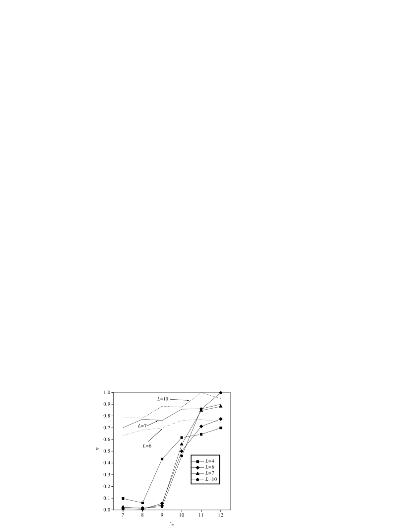
Figure 1: Distribution $p(s)$ of nearest level spacing. The lines without symbols correspond to the non-interacting Hamiltonian. The lines with symbols correspond to the full Hamiltonian [eq. 4].

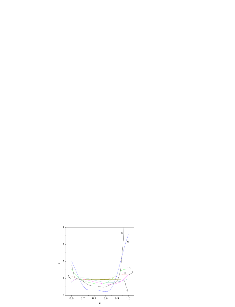
Figure 3: The ratio $\rho$ of the configuration-space inverse participation number $R$ with EEI to $R$ without. The numbers on the graph indicate the corresponding values of $r_{nn}$. $\rho=1$ for $r_{nn}=12$ (not shown). The energy scale is described in the text.

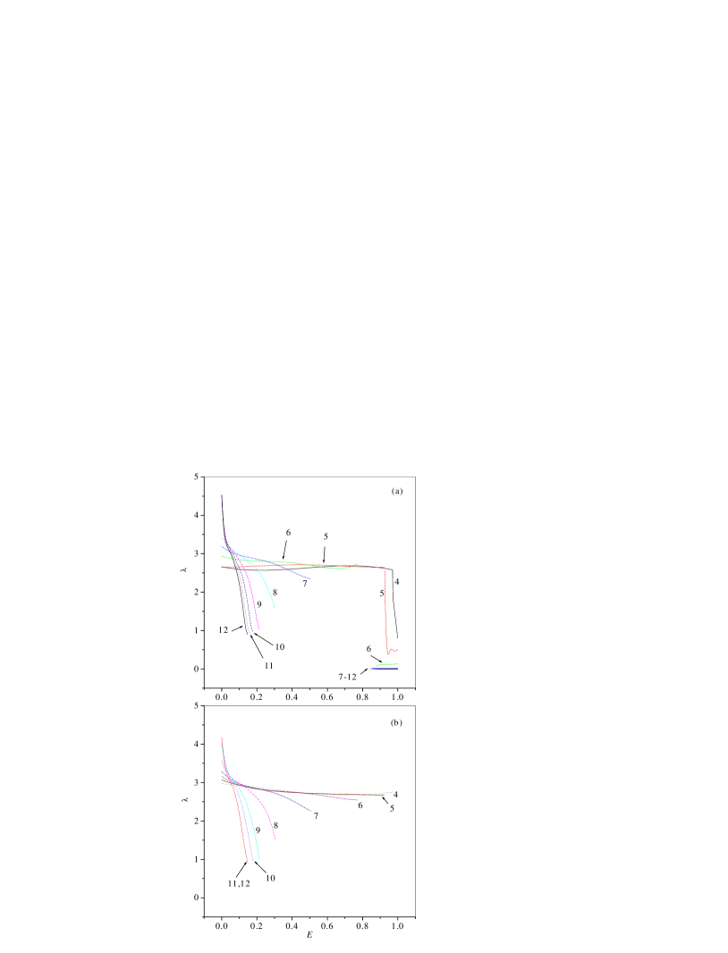
Figure 4: Fits for $\lambda(E)$ for (a) singlets, and (b) triplets with $L=7$. The numbers on the graph correspond to the values of $r_{nn}$. In (a) the upper bands coincide for $r_{nn}=7\textrm{-}12$; in (b) the plots for $r_{nn}=11,12$ coincide. The energy scale is described in the text.

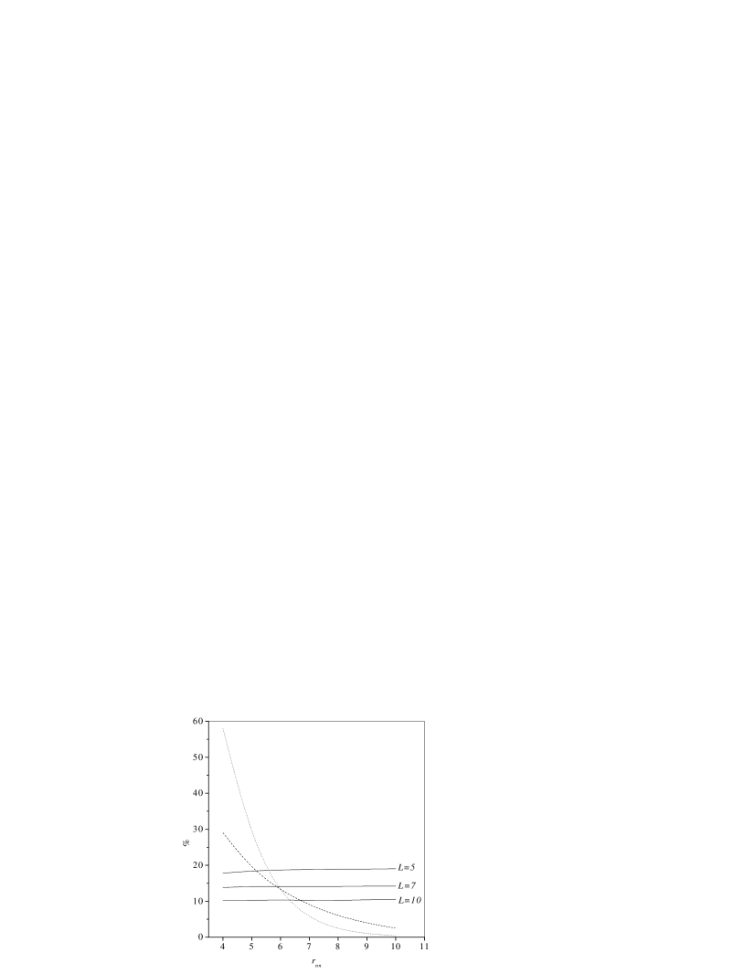
Figure 5: An evaluation of the importance of secondary processes relative to n-n tunneling. The solid lines are plots of $w/t_{nn}$. The dashed line is $S^{(\sqrt{2})}/S^{(1)}$ vs. $r_{nn}$ (the same plot for $L=5,7,10$), and the dotted line is $S^{(2)}/S^{(1)}$ vs. $r_{nn}$ (also the same plot for $L=5,7,10$). The vertical axis is given as a percent in all cases.

References

- [1] K. M. Frahm, Eur. Phys. J. B 10, 371 (1999); R. Römer, M. Leadbeater and M. Schreiber, Ann. Phys. 8, 675 (1999).
- [2] D. Shepelyansky, Phys. Rev. Lett. 73, 2607 (1994).
- [3] Y. Imry, Europhys. Lett. 30, 405 (1995).
- [4] M. Pollak and M. L. Knotek, Journal of Non-Cryst. Sol. 32, 141 (1979).
- [5] M. Pollak, Phil. Mag. B 42, 781 (1980).
- [6] J. Talamantes, M. Pollak and L. Elam, Europhys. Lett. 35, 511 (1996).
- [7] D. Belitz and T. R. Kirkpatrick, Rev. Mod. Phys. 66, 261 (1994).
- [8] J. Talamantes and A. Möbius, phys. stat. sol. (b) 205, 45 (1998).
- [9] F. Epperlein, M. Schreiber and T. Vojta, Phys. Rev. B 56, 5890 (1997).
- [10] T. Vojta, F. Epperlein and M. Schreiber, Phys. Rev. Lett. 81, 4212 (1998).
- [11] R. Berkovits and B. I. Shklovskii, J. Phys.: Condens. Matter 11, 779 (1999).
- [12] E. Cuevas, Phys. Rev Lett. 83, 140 (1999).
- [13] D. Shepelyansky, cond-mat/9905231 preprint (1999).
- [14] D. Shepelyansky, Ann. Phys 8, 665 (1999).
- [15] E. Cuevas, and M. Ortuño, Ann. Phy. 8, Spec. Issue SI 37 (1999).
- [16] D. Shepelyansky, Phys. Rev. B 61, 4588 (2000).
- [17] S. V. Kravchenko, G. V. Kravchenko, J. E. Furneaux, V. M. Pudalov and D. M. D’Iorio, Phys. Rev. B 50, 8039 (1994); S. V. Kravchenko, W. E. Mason, G. E. Bowker, J. E. Furneaux, V. M. Pudalov and M. D’Iorio, Phys. Rev. B 51, 7038 (1995); S. V. Kravchenko, D. Simonian, M. P. Sarachik, W. E. Mason and J. E. Furneaux, Phys. Rev. Lett. 77, 4938 (1996); D. Simonian, S. V. Kravchenko and M. P. Sarachik, Phys. Rev. B 55, R13 421 (1997); D. Simonian, S. V. Kravchenko, M. P. Sarachik and M. V. Pudalov, Phys. Rev. Lett. 79, 2304 (1997); D. Popović, A. B. Fowler and S. Washburn, Phys. Rev. Lett. 79, 1543 (1997).
- [18] see, e.g. B. Shklovskii, B. Shapiro, B. R. Sears, P. Lambrianides and H. B. Shore, Phys. Rev. B 47, 11487 (1993).
- [19] B. Georgeot and D. L. Shepelyansky, Phys. Rev. Lett. 79,4365 (1997).
- [20] Ph. Jacquod and D. L. Shepelyansky, Phys. Rev. Lett. 79,1837 (1997).
- [21] D. J. Thouless, Physics Reports 13, 93 (1974).
- [22] J. Talamantes and M. Pollak in Hopping and Related Phenomena, edited by O. Millo and Z. Ovadyahu (Racah Institute of Physics, Jerusalem) 1995.
- [23] see, e.g., N. F. Mott, Adv. Phys. 16, 49 (1967).
- [24] It should be pointed out that any conclusions reached from finite-size scaling behavior of computer size samples cannot be applied to experimental size samples because of self-screening. Without screening there cannot be a thermodynamic limit – but screening per force introduces into the problem a screening length, which precludes self-similarity and thus eliminates the possibility of a simple critical transition.
- [25] A. Barelli, J. Bellisard, Ph. Jacquod, D. Shepelyansky, Phys. Rev. Lett. 77, 4752 (1996).
- [26] M. Pollak, phys. status sol. (b) 205, 35 (1998).
- [27] J. Talamantes, M. Pollak, and I. Varga, phys. stat. sol. (b) 218, 119 (2000).
- [28] T. M. Klapwijk and S. Das Sarma, Solid State Communications 110, 581 (1999).
- [29] J. Talamantes and M. Pollak, Physics of Semiconductors, edited by D. J. Lockwood (World Scientific Publishing, Singapore) 1995.
- [30] The idea is that the EEI pushes electrons away from each other, thus clearing out the vicinity of occupied sites. This enhances the coherent transfer of electrons to nearby sites. This enhancement is absent in the non-interacting case.