Theory of superconductor with $\kappa$ close to $1/\sqrt{2}$

Abstract

As was firstly shown by E. Bogomolny, the critical Ginzburg-Landay (GL) parameter $\kappa=1/\sqrt{2}$ at which a superconductor changes its behavior from type-I to type-II, is the special highly degenerate point where Abrikosov vortices do not interact and therefore all vortex states have the same energy. Developing a secular perturbation theory we studied how this degeneracy is lifted when $\kappa$ is slightly different from $1/\sqrt{2}$ or when the GL theory is extended to the higher in $T-T_{c}$ terms. We constructed a simple secular functional, that depends only on few experimentally measurable phenomenological parameters and therefore is quite efficient to study the vortex state of superconductor in this transitional region of $\kappa$. Basing on this, we calculated such vortex state properties as: critical fields, energy of the normal-superconductor interface, energy of the vortex lattice, vortex interaction energy etc. and compared them with previous results that were based on bulky solutions of GL equations.

I Introduction

Although the Ginzburg-Landau (GL) theory covers all the variety of superconductors, both of the type I with GL parameter $\kappa<1/\sqrt{2}$ and of the type II with $\kappa>1/\sqrt{2}$, the most theoretical studies of the vortex state deal with the case of $\kappa\gg 1/\sqrt{2}$ since at $\kappa\gg 1/\sqrt{2}$ the GL equations are simplified substantially and also the grand majority of type-II superconducting materials, including High-Tc superconductors, correspond to this limit.

Studies of superconductors in the transitional region of small $\kappa\sim 1/\sqrt{2}$ done mostly in the 70-s were based on the solution of the full system of GL equations and require bulky calculations. Meanwhile, E. Bogomolny proposed in 1976 an elegant way to operate with similar problem of the string theory [1] and showed that at the special point $\kappa=1/\sqrt{2}$ the order of the equations can be reduced and all the vortex states with arbitrary located vortices have the same energy when the applied field is equal to the critical field $H_{c}$.

Historically the Bogomolny approach was done for the high-energy physics and the superconducting community was unaware of it even when L. Jacobs and C. Rebbi [2] reformulated the Bogomolny equations in terms of superconductivity and demonstrated that they can be written in a form of nonlinear electrostatic equations of the Boltzman plasma that we are calling as Bogomolny Jacobs and Rebbi (BJR) equation. Only very recently the Bogomolny method was used to study vortices in mesoscopic disks [3] and to calculate the structure of multi-quanta vortices [4] in superconductors with $\kappa=1/\sqrt{2}$.

In the present paper we derive a regular way to treat the vortex state of superconductors with $\kappa$ close to $1/\sqrt{2}$ basing on the BJR approach. Our basic idea is to consider the highly degenerate Bogomolny state at $\kappa=1/\sqrt{2}$, $H=H_{c}$ as zero approximation and then to account for deviation from this point via the secular perturbation method that lifts the degeneracy and selects the most stable vortex configuration. In Sec. III we give a brief overview of the Bogomolny method and then, in Sec. IV, present the solutions of BJR equation for the different vortex lattices. In Sec. V we develop the secular perturbation approach. The following perturbations can lift the degeneracy.

(i) Deviation of $\kappa$ from $1/\sqrt{2}$ that is accounted by a small parameter.

$$\gamma=\kappa^{2}-\frac{1}{2}\approx\sqrt{2}\kappa-1.$$ (1)

(ii) Deviation of the applied field from $H_{c}$.

(iii) Next in

$$t=T/T_{c}-1$$ (2)

corrections to the GL functional.

(iy) Thermal fluctuation effects.

(y) Finite size and demagnetization effects.

We consider only the first three contributions and show that they can be incorporated in a very simple secular functional that acts on the Bogomolny degenerate solutions and looks like a six-order polynomial for the amplitude of the order parameter. This functional depends only on few phenomenological parameters that can be found from experiment and that completely determine the behavior of superconductors with $\kappa\sim 1/\sqrt{2}$ in a magnetic field.

Certain properties of superconductors with $\kappa\sim 1/\sqrt{2}$ were calculated either from the GL theory extended to low temperatures or from the microscopic Gorkov equations. These calculations, overviewed in Sec. II, were however dealing either with cumbersome analytical expansions or with numerical computations that both are difficult to catch on. It is therefore of interest to recalculate these properties in a systematic perturbation way and compare them with the older results.

In Sec. VI we calculate the following parameters of a superconductor with $\kappa\sim 1/\sqrt{2}$:

a) Critical fields $H_{c1}$, $H_{c2}$ and $H_{c}$.

b) Energy of the NS interface.

c) Energy of the regular vortex lattice as function of the applied field.

d) Energy of the N-quanta vortex.

e) Vortex interaction that can have unconventional attractive character.

Basing on these calculations we discuss the possible scenarios of the normal-superconducting (N-S) transition in a magnetic field for a superconductor with $\kappa\sim 1/\sqrt{2}$ (Sec.VII) that occurs either directly (like in a type-I superconductor) or via formation of the intermediate vortex (V) state (like in a type-II superconductor). The actual scenario depends on the relative strength and sign of coefficients in the perturbation functional that can be extracted from experiment. We calculate the location of the triple point $L$ on the $H-T$ plane where the direct N-S transition splits into N-V and V-S transitions and a superconductor changes its behavior from type-I to type-II. The important feature is that, the N-V and V-S transitions close to point $L$ can be both continuous and discontinuous unlike the traditional type-II superconductor with $\kappa\gg 1/\sqrt{2}$. We calculated the location of tricritical points $T_{2}$ and $T_{1}$ where the N-V and V-S transitions change their character from continuous to discontinuous.

II Previous study

A Theory

Already in his pioneering work [5] Abrikosov noted that solution of the GL equations at $\kappa\sim 1/\sqrt{2}$ is a separate and quite complicate problem. Since that various related theoretical investigations that are partially reviewed in [6, 7, 8] were done. The first series of investigations dealt with an expansion of the BCS free energy close to $H_{c2}$ over a small parameter $H-H_{c2}$. The magnetic and thermodynamic properties of superconductor close to $H_{c2}$ were calculated for dirty [9, 10] and intrinsic [11] superconductors. The most complete calculations of this type are given in [12]. The possibility to have a discontinuous N-V transition in a superconductor with $\kappa\sim 1/\sqrt{2}$ was firstly indicated in [9].

On the basis of BCS theory Tewordt and Neumann calculated the low-temperature corrections to GL functional [13, 14, 15] and found the upper [16] and low [15] critical fields with an accuracy $t^{2}$ at arbitrary $\kappa$.

Basing on this extended GL functional, A. E. Jacobs [17] considered a superconductor with $\kappa\sim 1/\sqrt{2}$ and calculated the NS interface energy, the energy of single and double quantized vortex. He obtained that at certain conditions the vortices in a type-II superconductor attract each other and predicted the discontinuity of the V-S and N-V transitions. The analogous result was also obtained by Hubert [18] .

Großmann and Wissel [19] calculated the free energy of a superconductor with $\kappa\sim 1/\sqrt{2}$ close to $H_{c2}$ using the extended (although not complete) functional of Tewordt and Neumann. They founded a discontinuity of V-S transition in a limit of the dense vortex lattice. All the above conclusions were reproduced by Brandt [20] who developed a variational numerical method to solve the Gorkov’s equation for vortex lattices for all possible values of $H$, $T$ and $\kappa$.

Recently Ovchinnikov [21] carefully derived the coefficients of the extended GL functional from a microscopic theory for different types of the electron scattering. He considered an expansion of the free energy near $H_{c2}$ up to the order of $(H-H_{c2})^{3}$ and specified the case when at $\kappa\sim 1/\sqrt{2}$ the N-V transition has a discontinuous character.

In the present article we reproduce the above results in a more simple way, basing on the Bogomolny treatment of superconductors with $\kappa=1/\sqrt{2}$.

B Experiment

The superconducting metals Ta, Nb, In and Pb with $\kappa$ close to $1/\sqrt{2}$ were intensively studied in the 60-s and 70-s. The variation of $\kappa$ was achieved either by dissolving of foreign atoms of N, Tl, Bi or by preparation of samples with different defect concentration. We refer to magnetic [22] calorimetric [23] and neutron diffraction [24, 25] experiments in pure Nb ($\kappa\sim 0.85-0.96$), to magnetic measurements in TaN ($\kappa\sim 0.35-1.53$) [26], in Nb ($\kappa\sim 0.78-1.03$) [26] and in InBi ($\kappa\sim 0.76-1.46$) [27] and to direct observation of vortices in PbTl ($\kappa\sim 0.43-1.04$) [28] and in PbIn ($\kappa\sim 0.76-1.46$) [29, 30] by decoration. References to other related experiments can be fond in [6, 7].

The fact that the V-S transition can be of the first order at $\kappa\sim 1/\sqrt{2}$ was discovered already in the early magnetic and thermodynamic experiments [22, 23, 27]. The detailed magnetic study of a superconductor that changes its behavior from type I to type II was done for tantalum samples with some amount of dissolved nitrogen [26]. A discontinuity of the vortex lattice parameter at the V-S transition was observed in neutron-scattering experiments [24, 25].

The convincing confirmation of discontinuity of the V-S transition in superconductors with $\kappa\sim 1/\sqrt{2}$ was done by a direct observation the vortex domains inside the Meissner phase [28, 29, 30]. Such coexistence of different phases is known to be a signature of the first order transition between them. This intermediate-mixed domain structure was interpreted in [28] in terms of a long-range vortex attraction.

The discontinuity of the V-S transition provided by an attractive interaction between vortices is therefore a well established fact. Meanwhile the ground state of the vortex lattice and the configuration of domains of the mixed-intermediate phase are still unclear. Although the decoration experiments [6, 7, 28, 29, 30] demonstrate the very peculiar magnetic textures, including vortex segregation and clustering into lamellar and drop-like domains, no systematic study of this question that take into account the demagnetization and finite-size effects was done. We believe that our calculations of the vortex energy in the bulk superconductor with $\kappa\sim 1/\sqrt{2}$ can be extended to simulation of magnetic textures in the realistic finite-size samples.

III GL functional at $\kappa^{2}=1/2$ and BJR equation

In this Section we describe the Bogomolny procedure [1] that allows to simplify the GL functional and to reduce the order of the GL equations at $\kappa=1/\sqrt{2}$. Jacobs and Rebbi [2] formulated the Bogomolny equations in a simple form of the nonlinear Poisson equation that we shall call as BJR equation. We discuss the properties of the vortex solutions of the BJR equation and their interpretation in terms of electrons in Boltzman plasma given in [4].

We start from the conventional GL functional:

$${\cal F}=\alpha\left|\Psi\right|^{2}+\frac{g}{2}\left|\Psi\right|^{4}+K\left|{\bf D}\Psi\right|^{2}+\frac{B^{2}}{8\pi}-\frac{BH_{0}}{4\pi},$$ (3)

where

$\displaystyle\alpha=\alpha_{1}t,{\bf\quad D}=\nabla-i\frac{2e}{c\hbar}{\bf A,}\quad{\bf B}=rot{\bf A.}$

Refer first to the characteristic parameters of superconductor. In the uniform state the superconducting order parameter takes the equilibrium value:

$$\Psi_{0}=\left(-\frac{\alpha}{g}\right)^{1/2}.$$ (4)

Ratio of the penetration depth and coherence length:

$$\delta=\left(-\frac{c^{2}\hbar^{2}}{32\pi Ke^{2}}\frac{g}{\alpha}\right)^{1/2},\quad\xi=(-\frac{K}{\alpha})^{1/2}$$ (5)

gives the GL parameter:

$$\kappa=\frac{\delta}{\xi}=\frac{1}{(32\pi)^{1/2}}\frac{c\hbar g^{1/2}}{\left|e\right|K}.\$$ (6)

Thermodynamic critical field and the upper critical field are written as:

$$H_{c}=-\left(\frac{4\pi}{g}\right)^{1/2}\alpha,\quad H_{c2}=-\frac{c\hbar}{2\left|e\right|D}\alpha=\sqrt{2}\kappa H_{c}.$$ (7)

Note that the commonly used expression for the low critical field:

$$H_{c1}=\frac{\Phi_{0}}{4\pi\delta^{2}}\ln\kappa=H_{c}\frac{\ln\kappa}{\sqrt{2}\kappa}.$$ (8)

is valid for $\kappa\gg 1/\sqrt{2}$ and is not applicable in our case. Corresponding expression for $H_{c1\text{ }}$at $\kappa\sim 1/\sqrt{2}$ will be obtained in Sec. VI. Introduce now the dimensionless variables that are slightly different from the commonly used in the GL theory:

$$\psi = \frac{\Psi}{\Psi_{0}},\qquad r=\frac{R}{\delta\sqrt{2}},$$ (9)

$$b = \sqrt{2}\kappa\frac{B}{H_{c}},\qquad h_{0}=\sqrt{2}\kappa\frac{H_{0}}{H_{c}},\qquad{\bf a=}\ \frac{\kappa{\bf A}}{\delta H_{c}},$$ (10)

$$f = \frac{{\cal F}}{H_{c}^{2}/8\pi}\kappa^{2}+\kappa^{2}.$$ (11)

The GL functional (3) in this variables takes the form:

$$\ f=\kappa^{2}(\left|\psi\right|^{2}-1)^{2}+\left|(\ \nabla-i{\bf a})\psi\right|^{2}+\ (\frac{b^{2}}{2}-bh_{0}).\$$ (12)

It is convenient to use the complex variables:

$$\zeta,\overline{\zeta} = x\pm iy,$$ (13)

$$\partial,\overline{\partial} = \frac{1}{2}(\nabla_{x}\mp i\nabla_{y}),$$ (14)

$$a,\overline{a} = \frac{1}{2\ }(a_{x}\mp ia_{y})$$ (15)

in which the GL functional is written as:

$$\ f = \ 2\left|(\partial-ia)\psi\right|^{2}+\ 2\left|(\overline{\partial}-i\overline{a})\psi\right|^{2}$$ (17)

$$+\kappa^{2}(\left|\psi\right|^{2}-1)^{2}\ +\ (\frac{b^{2}}{2}-bh_{0})\ \$$

To catch the special properties of the GL functional at $\kappa=1/\sqrt{2}$ one can integrate the first term in (17) by parts. Using that:

$$\int f\overline{\partial}gdS=-\int g\overline{\partial}fdS+\frac{i}{2}\oint fgd\overline{\zeta}$$ (18)

and that:

$$b=-2i(\partial\overline{a}-\overline{\partial}a)$$ (19)

one gets the substitution:

$$2\left|(\partial-ia)\psi\right|^{2}\rightarrow 2\left|(\overline{\partial}-i\overline{a})\psi\right|^{2}+\left|\psi\right|^{2}b.$$ (20)

We neglect the contribution of the surface currents that are important for finite-size effects considered in [3]. Finally, one comes to the alternative expression for $f$:

$$f = 4\left|(\overline{\partial}-i\overline{a})\psi\right|^{2}+\frac{1}{2}\left(b+\left|\psi\right|^{2}-1\right)^{2}$$ (22)

$$+\ \gamma(\left|\psi\right|^{2}-1)^{2}\ +(1-h_{0})b,$$

where $\gamma=\kappa^{2}-1/2$. When $\gamma=0$ and $h_{0}=1$ (i.e. $H=H_{c}$) the functional (22) reduces to the sum of two square terms. The absolute minimum is achieved when both these terms are equal to zero i.e. when the following equations are satisfied:

$$(\overline{\partial}-i\overline{a})\psi=0$$ (23)

and

$$1-\psi\overline{\psi}=-2i(\partial\overline{a}-\overline{\partial}a)=b.$$ (24)

Substitution of $\overline{a}$ from (23):

$$\overline{a}=-i\overline{\partial}\ln\psi$$ (25)

to (24) gives the BJR equation:

$$\frac{1}{2}\nabla^{2}\ln\left|\psi\right|^{2}=\left|\psi\right|^{2}-1+2\pi\sum N_{i}\delta({\bf r}-{\bf r}_{i}).$$ (26)

Firstly introduced in [4] the $\delta$-function terms correspond to the $N_{i}$-quanta vortices located at ${\bf r}={\bf r}_{i}$ where $\psi$ gets the phase wind $2\pi N_{i}$ and $\ln\left|\psi\right|$ has a $\ln r^{N}\,$singularity. As follows from Eq. (24) the distribution of magnetic field inside a sample is uniquely related with the amplitude of the order parameter:

$$b({\bf r})=1-\left|\psi({\bf r})\right|^{2}.$$ (27)

The BJR equation can be alternatively written as:

$$\nabla^{2}\varphi=e^{2\varphi}-1+2\pi\sum N_{i}\delta({\bf r}-{\bf r}_{i}).$$ (28)

where $\varphi=\ln\left|\psi\right|$. This form has a simple interpretation [4]. It describes the screening of electrons in a classical Boltzman plasma that consists of the positive ionic background with potential $1/4\pi$.

BJR equation (26) defines the amplitude of the superconducting order parameter $\left|\psi({\bf r})\right|$ and the magnetic field $b({\bf r})\$at $\gamma=0$   and at $h_{0}=1$ as a function of position of the vortices ${\bf r}_{1}...{\bf r}_{n}$. All these vortex solutions correspond to the absolute minimum of the functional (22) and, therefore, $\gamma=0$ and $h_{0}=1$ is a special highly degenerate point where all the vortex states have the same energy.

This infinite degeneracy over ${\bf r}_{1}...{\bf r}_{n}$ is lifted if one goes either beyond $\gamma=0$, $h_{0}=1$ or beyond the GL approximation. When $\gamma=0$ and $h_{0}>1$ the absolute minimum of (22) is the normal state with $b=h_{0}$ and $\left|\psi\right|=0$. When $\gamma=0$ and $h_{0}<1$ the absolute minimum of (22) is the uniform superconducting state with $b=0$ and $\left|\psi\right|=1$. To find the vortex states when $\gamma\neq 0$ one should account for the term $\gamma(\left|\psi\right|^{2}-1)^{2}$ as the secular perturbation that lifts the degeneracy. This will be done in Sec. V together with account of the low temperature corrections to the GL functional.

IV Vortex state at $\kappa^{2}=1/2$

A General

In this Section we discuss a particular class of solutions of BJR equation (26) when $N-$ quanta vortices are packed into the regular lattice with basis vectors ${\bf a}_{1},{\bf a}_{2}$. We will need these solutions in Sec. VI as zero approximation of the perturbation theory to find the most stable vortex configuration beyond the Bogomolny point. The unit cell area $S=a_{1}a_{2}\sin\alpha$ ($\alpha={\bf a}_{1}{}^{\wedge}{\bf a}_{2}$) carries the flux $2\pi N$ and therefore is related with the average induction as:

$$S=2\pi N/\overline{b}.$$ (29)

The value of $\overline{b}$ and $S$ varies from $\overline{b}=0$, $S=\infty$ (almost non-overlapping vortices) to $\overline{b}=1$, $S=2\pi N$ (dense vortex lattice). We consider both the limits analytically. We use a numerical procedure to treat the case of an arbitrary lattice.

B One vortex

The axially-symmetric distribution of the order parameter $g_{N}(r)=\left|\psi(r)\right|$ inside the $N$-quanta vortex is calculated from the radial version of BJR equation (26):

$$g_{N}^{\prime\prime}=\frac{g_{N}^{\prime 2}}{g_{N}}-\frac{g_{N}^{\prime}}{r}+g_{N}^{3}-g_{N}$$ (30)

with the boundary conditions: $g_{N}(0)=0$, $g_{N}(\infty)=1$ and asymptotes:

$$g_{N} \simeq B_{N}r^{N}:\qquad\qquad\qquad r\rightarrow 0,$$ (31)

$$g_{N} \simeq 1-A_{N}\frac{e^{-\sqrt{2}r}}{\sqrt{r}}:\qquad r\rightarrow\infty.$$ (32)

We solved (30) numerically for $N=1$ and got $B_{1}\approx 0.9$ and $\ A_{1}\approx 1.6$.

To find the vortex solution at $N>1$ it is more convenient to use the new function $v_{N}(r)=g_{N}^{1/N}(r)$ that satisfies the equation:

$$v_{N}^{\prime\prime}=\frac{v_{N}^{\prime 2}}{v_{N}}-\frac{v_{N}^{\prime}}{r}+\frac{1}{N}v_{N}^{2N+1}-\frac{1}{N}v_{N}$$ (33)

and has a linear behavior $\sim B_{N}^{1/N}r$ at $r\rightarrow 0$. The analytical expression for $g_{N}(r)$ at $N\gg 1$ was obtained in [4]. In dimensionless units (11) it is written as:

$$g_{N}=\left(\frac{r}{r_{N}}\right)^{n}e^{-\frac{1}{4}(r^{2}-r_{N}^{2})}\quad r<r_{N}.$$ (34)

The size of the vortex core

$$r_{N}\approx\sqrt{2N}$$ (35)

is estimated from that, the almost uniform magnetic field $h_{0}=1$, distributed inside the vortex area $\pi r_{N}^{2}$ results to the flux $2\pi N$.

C Separated vortices and diluted lattice

The magnetic flux of slightly overlapping vortices can be written as the superposition of fluxes of separate vortices:

$$b({\bf r})=\sum_{i}b_{N}({\bf r}-{\bf r}_{i})=\sum_{i}\left(1-g_{N}^{2}(i)\right),$$ (36)

where $g_{N}(i)=g_{N}(\left|{\bf r}-{\bf r}_{i}\right|{\bf)}$ is the solution of (30). Then, the amplitude of the order parameter is written as:

$$\left|\psi({\bf r,r}_{1}...{\bf r}_{N}{\bf)}\right|^{2}=1-b({\bf r})=1+\sum_{i}\left(g_{N}^{2}(i)-1\right).$$ (37)

D Vortex bunch

Consider now the group of $N$ vortices located close to the origin such that $\left|{\bf r}_{i}\right|\ll 1$. This vortex bunch can be viewed as the $N-$quanta vortex $g_{N}(r)$ with the split core. By direct substitution one proves that the corresponding solution of equation (28) within the accuracy $O(\max\left|{\bf r}_{i}\right|^{2})$ is given by:

$$\varphi({\bf r},{\bf r}_{1}...{\bf r}_{N}) = \frac{1}{N}\sum_{i}\varphi_{N}({\bf r}-{\bf r}_{i})$$ (38)

$$\approx \varphi_{N}(r{\bf)+}\frac{1}{2N}\sum_{i}({\bf r}_{i}{\bf\nabla})^{2}\varphi_{N}(r{\bf),}$$ (39)

where $\varphi_{N}(r)=\ln\left|g_{N}(r)\right|$, $\varphi({\bf r},{\bf r}_{1}...{\bf r}_{N})=\ln\left|\psi({\bf r},{\bf r}_{1}...{\bf r}_{N})\right|$; the origin being taken in the center of the vortex gravity such that $\Sigma_{i}{\bf r}_{i}=0$.

With the same accuracy the order parameter is written as:

$$\left|\psi({\bf r},{\bf r}_{1}...{\bf r}_{N})\right|=g_{N}(r)+\frac{1}{2N}g_{N}(r)\sum_{i}({\bf r}_{i}{\bf\nabla})^{2}\ln g_{N}(r).$$ (40)

E Dense lattice

The order parameter of the dense 1-quanta vortex lattice is presented by the Abrikosov solution close to $H_{c2}$:

$$\psi_{0}({\bf r)}=A(\overline{b})\theta(\overline{z}\sqrt{\overline{b}\tau^{\prime\prime}/2\pi},\tau)e^{-\overline{b}y^{2}/2},$$ (41)

where:    $\tau=\tau^{\prime}+i\tau^{\prime\prime}=a_{2}e^{i\alpha}/a_{1}$ is the geometrical parameter of the lattice cell (for square lattice $\tau=i$; for triangular lattice: $\tau=e^{i\pi/3}$) and $\theta$ is the Jacobi theta-function:

$$\theta(\overline{z},\tau)=2\sum_{n=0}^{\infty}(-1)^{n}e^{i\pi\tau(n+1/2)^{2}}\sin[\pi(2n+1)\overline{z}].$$ (42)

Function $\psi_{0}({\bf r)}$ satisfies the linear equation:

$$\overline{b}\nabla^{2}\ln\left|\psi_{0}\right|=-1+2\pi\sum\delta({\bf r}-{\bf r}_{i}),$$ (43)

that close to $H_{c2}$ coincides with BJR equation in a limit $<\left|\psi\right|^{2}>\rightarrow 0$, $\overline{b}\rightarrow 1$. To find the normalization coefficient $A(\overline{b})\sim(1-\overline{b})^{1/2}$ one should treat the nonlinear part of BJR equation as a perturbation.

The $N$-quanta lattice solution with unit cell area $2\pi N$ can be written in the analogous way:

$$\psi_{0}({\bf r)}=A_{N}(\overline{b})\theta^{N}(\overline{z}\sqrt{\overline{b}\tau^{\prime\prime}/2\pi N},\tau)e^{-\overline{b}y^{2}/2}.$$ (44)

F Arbitrary lattice (numerical solution)

We performed the numerical integration of BJR equation for square and triangular vortex lattices with $N=1,2$ in a whole interval of $0<\overline{b}<1$ presented it in a more suitable form. First we pick the zeroes of the order parameter via the special multiplier $\psi_{0}({\bf r)}$ that was taken as (41) for $N=1$ or as (44) for an arbitrary $N$ and present the order parameter in the form: $\psi({\bf r)=}\left|\psi_{0}({\bf r)}\right|\cdot\left|\psi^{\prime}({\bf r)}\right|$. The new equation for function $\left|\psi^{\prime}({\bf r)}\right|$ has no singular $\delta$-function terms and is written as:

$$\frac{1}{2}\nabla^{2}\ln\left|\psi^{\prime}\right|^{2}=\left|\psi_{0}\right|^{2}\left|\psi^{\prime}\right|^{2}-(1-\overline{b}).$$ (45)

Taking $\varphi^{\prime}=\ln\left|\psi^{\prime}\right|$ we present (45) in a form:

$$\nabla^{2}\varphi^{\prime}=\left|\psi_{0}\right|^{2}e^{2\varphi^{\prime}}-(1-\overline{b}).$$ (46)

This nonlinear Poisson-like equation can have the periodic solution only if the electroneutrality condition is satisfied:

$$1-\overline{b}=<\left|\psi_{0}\right|^{2}e^{2\varphi^{\prime}}>.$$ (47)

Taking into account (47) and performing the rescaling ${\bf r}\rightarrow{\bf r}\cdot(2\pi N/\overline{b})^{1/2}$ we map Eq. (46) onto

$$\nabla^{2}\varphi^{\prime}=\Lambda\ (\frac{\left|\psi_{0}({\bf r})\right|^{2}e^{2\varphi^{\prime}}}{<\left|\psi_{0}({\bf r})\right|^{2}e^{2\varphi^{\prime}}>}-1),$$ (48)

that is defined for the parallelogram of the fixed area $S=1$ with periodic boundary conditions. The parameter of the equation

$$\Lambda=2\pi N\left(\frac{1}{\overline{b}}-1\right)$$ (49)

varies from $0$ at $H_{c2}$ to $\infty$ at $H_{c1}$.

The problem was solved for the square and triangular vortex lattices with $N=1,2$ using the Matlab PDE Toolbox by the finite element method with the adaptive mesh refinement and with the rapidly converging Gauss-Newton iterations that were used to account the non-linear right-hand side of (48). For details of the numerical method see Ref. [31]. The obtained solutions were verified by the direct substitution them back to (48).

G Normal-superconducting interface

The profile of the NS interface is usually considered in two limit cases: when $\kappa\rightarrow\infty$ or when $\kappa\rightarrow 0$. It appears, however, that the NS profile can be found exactly at $\kappa=1/\sqrt{2}$ by integration of the equation (28) that in 1D case looks like:

$$\varphi^{\prime\prime}=e^{2\varphi}-1.$$ (50)

The first integral of (50):

$$(\varphi^{\prime})^{2}=e^{2\varphi}-2\varphi-1$$ (51)

alternatively can be written as:

$$(\left|\psi\right|^{\prime})^{2}=\left|\psi\right|^{4}-\left|\psi\right|^{2}(1+\ln\left|\psi\right|^{2}).$$ (52)

The integration constant in (51), (52) was chosen to satisfy the NS interface boundary conditions:

$$\left|\psi\right| = 0,\text{\quad}d\left|\psi\right|/dx=0\text{\quad when }x\rightarrow-\infty,$$ (53)

$$\left|\psi\right| = 1,\text{\quad}d\left|\psi\right|/dx=0\text{\quad when }x\rightarrow\infty.$$ (54)

Further integration of (52) gives the implicit form of $\left|\psi(x)\right|$ at the NS interface:

$$x=\int^{\left|\psi\right|}\frac{dy}{\sqrt{y^{4}-y^{2}(1+\ln y^{2})}}.$$ (55)

V Perturbation theory

To find the most stable configuration of vortices beyond the infinitely degenerate point $\gamma=0$, $h_{0}=1$ of Bogomolny functional (22) we construct the secular perturbation functional that acts on the (zero order) degenerate solutions $\left|\psi({\bf r},{\bf r}_{1}...{\bf r}_{n})\right|$ of (26) and selects the vortex configuration ${\bf r}_{1}...{\bf r}_{n}$ having the lowest energy.

The perturbation for $\gamma$ and $h$ were given already by two last terms in (22). To find the perturbation for $t$ one should extend the GL functional to low temperatures. Tewordt [13, 14, 16] and Newman and Tewordt [15] were the first who proposed the complete form of such extension. We will use the analogous functional given in a more recent publication [21]:

$${\cal F} = a\left|\Psi\right|^{2}+\frac{g}{2}\left|\Psi\right|^{4}+K\left|{\bf D}\Psi\right|^{2}+\frac{B^{2}}{8\pi}-\frac{BH_{0}}{4\pi}$$ (58)

$$+\frac{u}{3}\left|\Psi\right|^{6}+R^{\prime}\left|\Psi\right|^{2}\left|{\bf D}\Psi\right|^{2}+R^{\prime\prime}(\nabla\left|\Psi\right|^{2})^{2}+P\left|{\bf D}^{2}\Psi\right|^{2}$$

$$LB^{2}\left|\Psi\right|^{2}+Qrot^{2}{\bf B.}$$

The last term $rot^{2}{\bf B}$ was written in [21] in the equivalent form $-i\,rot{\bf B}(\overline{\Psi}{\bf D}\Psi-\Psi\overline{{\bf D}}\overline{\Psi})$.

To account for all the perturbations of the order of $t$ one should assume that coefficients $u$, $R^{\prime}$, $R^{\prime\prime}$, $P$, $L$, and $Q$ are temperature independent whereas coefficients $\alpha$, $g$ and $K$ are expanded in $t$ as:

$$\alpha = (\alpha_{1}+\alpha_{2}t)t,$$ (59)

$$g = g_{0}+g_{1}t,$$ (60)

$$K = K_{0}+K_{1}t.$$ (61)

The microscopic BCS values of these coefficients are given in Appendix.

The combination $g^{1/2}/K$ that enter in (22) as defined by (6) parameter $\kappa$ becomes now temperature dependent. We keep a notation $\kappa=(1+\gamma)/\sqrt{2}$ for the temperature independent part of (6) and take $\sigma t/\sqrt{2}$ with

$$\sigma=g_{1}/g_{0}-2K_{1}/K_{0}$$ (62)

as a linear in $t$ contribution to (6). Therefore the third term in (22) contains both the perturbation in $\gamma$ and in $t$ and is written as:

$$\ (\gamma+\sigma t)(\left|\psi\right|^{2}-1)^{2}.$$ (63)

Other perturbation terms of (58) can be substantially simplified if one takes into account that they are operating with solutions of BJR equation. The final form of these terms in dimensionless variables and corresponding dimensionless coefficients are given in Table I. We present also the numerical values of these coefficients calculated from microscopic BCS theory given in Appendix. We comment now, how the perturbation terms were obtained.

1) The term $P\left|{\bf D}^{2}\Psi\right|^{2}$ is rewritten in dimensionless units as:

$$-t\mu\left|2[(\partial-ia)(\overline{\partial}-i\overline{a})+(\overline{\partial}-i\overline{a})(\partial-ia)]\psi\right|^{2}$$ (64)

$$= -t\mu\left|4(\partial-ia)(\overline{\partial}-i\overline{a})\psi+2i(\partial\overline{a}-\overline{\partial}a)\psi\right|^{2}.$$ (65)

Because of (23) and (24) the first term in brackets vanishes and the second term is equal to:

$$-t\mu b^{2}\left|\psi\right|^{2}=-t\mu\left|\psi\right|^{2}(1-\left|\psi\right|^{2})^{2}.$$ (66)

2) The term $R^{\prime}\left|\Psi\right|^{2}\left|{\bf D}\Psi\right|^{2}$ is rewritten in dimensionless units as:

$$-2t\rho^{\prime}\left|\psi\right|^{2}\left(2\left|(\partial-ia)\psi\right|^{2}+2\left|(\overline{\partial}-i\overline{a})\psi\right|^{2}\right)$$ (67)

$$= -2t\rho^{\prime}(4t\left|\psi\right|^{2}\left|(\overline{\partial}-i\overline{a})\psi\right|^{2}-ia\overline{\partial}\left|\psi\right|^{4}+i\overline{a}\partial\left|\psi\right|^{4}).$$ (68)

The first term in brackets vanishes and two other ones can be integrated by parts. This leads to:

$$-t\rho^{\prime}\left|\psi\right|^{4}\cdot 2i(\overline{\partial}a-\partial\overline{a}) = -t\rho^{\prime}b\left|\psi\right|^{4}$$ (69)

$$= -t\rho^{\prime}\left|\psi\right|^{4}(1-\left|\psi\right|^{2}).$$ (70)

3) The term $Qrot^{2}{\bf B}$ in dimensionless units is rewritten as:

$$-t\tau\,rot^{2}({\bf z}b)=-t\tau(\nabla\left|\psi\right|^{2})^{2}.$$ (71)

Multiplying (26) by $\left|\psi\right|^{4}$ and integrating by parts we find that $(\nabla\left|\psi\right|^{2})^{2}$ can be substituted as:

$$(\nabla\left|\psi\right|^{2})^{2}\rightarrow\left|\psi\right|^{4}-\left|\psi\right|^{6},$$ (72)

the same substitution was also done for the term $R^{\prime\prime}(\nabla\left|\Psi\right|^{2})^{2}$.

Collecting all the above contributions together and omitting the nonessential constant contribution $1+\gamma+\sigma t-h_{0}$ we came to the resulting perturbation functional:

$$f^{\prime}=(h_{0}-h_{c2})\left|\psi\right|^{2}+(\gamma-c_{4}t)\left|\psi\right|^{4}-c_{6}t\left|\psi\right|^{6},$$ (73)

where parameters$\ c_{i}$ are given in Table II. The instability field:

$$h_{c2}=1+2\gamma+c_{2}t.$$ (74)

corresponds to the upper critical field that we discuss below.

Perturbation functional (73) is the principal result of the present work. It allows to calculate the properties of superconductor with low $\gamma$ and select the most stable vortex configuration at given $\gamma$, $h_{0}$ and $t$. Although functional (73) resembles the extended form of the GL functional, it is defined for the restricted set of infinitely degenerate vortex solutions $\left|\psi({\bf r},{\bf r}_{1}...{\bf r}_{n})\right|$ of BJR equation (26). The important advantage of the functional (73) is that, it depends only on few parameters: $h_{c2}$, $c_{4}$ and $c_{6}$ that are the combinations of the coefficients of the extended GL functional (58) as it is given in Table II. Moreover, it is not necessary to know the coefficients in the starting functional (58) at all. These parameters can be considered as the phenomenological ones. As will be shown in Sec. VII they can be found from experiment.

The occurring vortex state depends on sign and relative strength of the coefficients $\gamma-c_{4}t$ and $-c_{6}$ that can be both positive and negative since $t<0$ and parameter $\gamma$ changes the sign when $\kappa$ goes though $1/\sqrt{2}$. The realistic values of $c_{4}$ and $c_{6}$ will be discussed in Sec. VII.

(i) When both $\gamma-c_{4}t$ and $-c_{6}t$ are positive the magnetic behavior of the superconductor corresponds to the generic scenario for a superconductor of type II. The dense vortex lattice (41) appears continuously from the normal state $\left|\psi\right|=0$ at upper critical field $h_{c2}$ when the quadratic term $(h_{0}-h_{c2})\left|\psi\right|^{2}$ in (73) becomes unstable. The amplitude $\Delta^{2}=<\left|\psi({\bf r})\right|^{2}>$ of the vortex state and the intervortex distance increase with decreasing of the applied field. Below the low critical field $h_{c1}$ that will be calculated in Sec.VI B all the vortices continuously leave the superconductor and the uniform Meissner state with $\left|\psi\right|=1$ becomes stable.

(ii) When both $\gamma-c_{4}t$ and $-c_{6}t$ are negative, the functional (73) corresponds to a type-I superconductor. There are only two competing local minima of (73): the normal state with $\left|\psi\right|=0$ and energy

$$f_{n}^{\prime}=0,$$ (75)

and the uniform superconducting Meissner state with $\left|\psi\right|=1$ and energy:

$$f_{s}=h_{0}-h_{c2}+\gamma-(c_{4}+c_{6})t.$$ (76)

The discontinuous transition between them occurs at the thermodynamic critical field $h_{c}$

$$h_{c}=1+\gamma+(c_{2}+c_{4}+c_{6})t.$$ (77)

that is found by equating (75) and (76).

(iii) We investigate the case when coefficients $\gamma-c_{4}t$ and $-c_{6}t$ have different signs in Sec. VII. It will appear that, depending on the situation, both N-V and V-S transition can be either continuous (as in conventional superconductors with $\kappa\gg 1/\sqrt{2}$) or discontinuous. This situation is accessible experimentally either by variation of $\gamma$ or by variation of $t$.

VI Vortex state: energy and critical fields

A Energy of the vortex lattices and higher critical field

The energy of the regular $N$-quanta lattice (73) can be written in terms of the amplitude of the order parameter $\Delta^{2}=<\left|\psi\right|^{2}>$ as:

$$f^{\prime} = (h_{0}-h_{c2})\Delta^{2}$$ (79)

$$+(\gamma-c_{4}t)\beta_{4}(\Delta)\Delta^{4}-c_{6}t\beta_{6}(\Delta)\Delta^{6},$$

where $\beta_{n}^{(N)}(\Delta)$ are the structural factors:

$$\beta_{n}^{(N)}(\Delta)=\frac{<\left|\psi\right|^{n}>}{<\left|\psi\right|^{2}>^{n/2}},$$ (80)

that depend both on the amplitude $\Delta$ and on the lattice geometry.

Minimization of (79) over $\Delta$ gives the complete information about thermodynamic and magnetic properties of vortex lattice in a superconductor with $\kappa\sim 1/\sqrt{2}$, provided the dependencies $\beta_{n}^{(N)}(\Delta)$ are known. We found $\beta_{n}^{(N)}(\Delta)$ in the whole region of $\Delta\$($0<\Delta<1$) using the numerical solutions of (26) for square and triangular vortex lattices with $N=1,2$ outlined in Sec. IV F. The results are shown in Fig.1 as function of magnetic induction

$$\overline{b}=1-\Delta^{2}.$$ (81)

The values of $\beta_{n}^{(1,2)}$ at $\Delta\rightarrow 0$ (i.e. in vicinity of $h_{c2}$) are given in Table III. Parameter $\beta_{4}^{(N)}(0)\$corresponds to the parameter $\beta$ introduced in the original publication of Abrikosov [5]. Close to $h_{c1}$ (where $\Delta\rightarrow 1$) the factors $\beta_{n}^{(N)}$ are tending to $1$. The  corresponding asymptotic expression will be given in Sec. VI B.

Functional (79) close to $h_{c2}$ can be interpreted as a Landau expansion of the vortex state energy over the amplitude $\Delta$. When $\gamma>c_{4}t$ the quartic in $\Delta$ term is positive and the conventional second order transition occurs at $h_{c2}$. When $\gamma<c_{4}t$ the transition occurs in a discontinuous way either to the finite-amplitude vortex state or directly to the Meissner state. The concrete realization of this transition depends on the relative values of $c_{6}$ and $c_{4}$ and will be discussed in Sec. VII.

Condition:

$$\gamma-c_{4}t=0$$ (82)

defines the tricritical point $T_{2}$ where the discontinuity of N-V transition appears. The discontinuity field $h_{c2}^{\ast}$ is large than the critical field $h_{c2}$.

Functional (79) can be alternatively written in terms of $\overline{b}$ as:

$$f^{\prime} = (2\gamma+c_{2}t)(h_{0}-1)+(h_{0}-h_{c2})(h_{c2}-\overline{b})$$ (84)

$$+(\gamma-c_{4}t)\beta_{4}(\overline{b})(h_{c2}-\overline{b})^{2}-c_{6}t\beta_{6}(\overline{b})(h_{c2}-\overline{b})^{3}.$$

Minimization of $f^{\prime}$ over $\overline{b}$ gives the induction $\overline{b}(h_{0})$ and the lattice energy $f^{\prime}(h_{0})$. Comparing the energies of square and triangular lattices with $N=1,2$ at given $h_{0}$ ($h_{c1}<h_{0}<h_{c2}$) we established that one-quanta triangular vortex lattice always possess the lowest energy. However close to $h_{c1}$ the energies of different lattices coincide within the calculation accuracy and this conclusion becomes less certain.

B Diluted lattice, low critical field and vortex interaction

1 Energy of the diluted vortex lattice

We consider now the diluted lattice of slightly overlapping $N$-quanta vortices assuming that the distance $l$ between them is much larger then the coherence length (i.e. $l\gg 1$). Such limit usually occurs close to the low critical field $h_{c1}$. In this approximation the energy of the system is written as:

$$f^{\prime}=f_{s}^{\prime}+\frac{\overline{b}}{2\pi N}\varepsilon_{N}+\frac{m}{2}\frac{\overline{b}}{2\pi N}U_{int}(l)-h_{0}\overline{b},$$ (85)

where the background energy of the uniform Meissner state $f_{s}^{\prime}$ is given by (76), $\ \varepsilon_{N}$  is the one-vortex energy, $\overline{b}/2\pi N$ is the density of vortices and $-h_{0}\overline{b}$ is the interaction of the vortex with an external field. The term $U_{int}(l)$ represents the interaction between the nearest neighbor vortices. The factor $\ m$ gives the lattice coordination number: $m=6$ for the triangular lattice and $m=4$ for the square lattice. The inter-vortex distance $l$ is uniquely related with the vortex concentration $2\pi N/\overline{b}$ and geometry of the lattice as:

$$l_{\square}=(2\pi N/\overline{b})^{1/2},\quad l_{\Delta}=(4\pi N/\overline{b}\sqrt{3})^{1/2}.$$ (86)

The type of the V-S transition depends on sign of the long-range vortex interaction $U_{int}(l)$ that, as will be shown below, can be both repulsive and attractive.

When $U_{int}(l)>0$ the situation is the same as for a superconductor of type-II: the V-S transition occurs in a continuous way at the low critical field $h_{c1}$ that is calculated from the vortex energy $\varepsilon_{N}$. The latter can be written on the basis of (73) as:

$$\varepsilon_{N}=2\pi N[(1+2\gamma+c_{2}t)-\zeta_{4}^{(N)}(\gamma-c_{4}t)+\zeta_{6}^{(N)}c_{6}t].$$ (87)

The structural factors for the $N$-quanta vortex:

$$\zeta_{n}^{(N)}=\frac{1}{N}\int_{0}^{\infty}(1-g_{N}^{n})rdr$$ (88)

are found from integration of the numerical solution $g_{N}(r)$ of Eq. (30) and are given in Table III. Note also that:

$$\zeta_{2}^{(N)}=\frac{\overline{b}}{2\pi N}=1\text{.}$$ (89)

Factors $\zeta_{n}^{(N)}$ for large $N$ will be calculated in Sec. VI C. Lattice factors $\beta_{n}^{(N)}$ (80) can be expressed via $\zeta_{n}^{(N)}$ as:

$$\beta_{n}^{(N)}=\frac{1-\zeta_{n}^{(N)}\overline{b}}{(1-\overline{b})^{n/2}}\quad(\overline{b}\rightarrow 0).$$ (90)

The $N$-quanta vortices penetrate into a sample when the positive energy $\varepsilon_{N}$, required for the vortex  creation is compensated by the negative magnetic contribution $-h_{0}\overline{b}$ i.e. above the critical field:

$$h_{c1}^{(N)} = \frac{\varepsilon_{N}}{2\pi N}=1+(2-\zeta_{4}^{(N)})\gamma$$ (92)

$$+(c_{2}+\zeta_{4}^{(N)}c_{4}+\zeta_{6}^{(N)}c_{6})t.$$

The low critical field is defined as the lowest field when penetration of vortices becomes favorable:

$$h_{c1}=\min\{h_{c1}^{(N)}\}_{N}.$$ (93)

It appears that only the 1-quanta vortices can appear in a continuous way since condition of formation of 2-quanta vortices written as $h_{c1}^{(2)}<h_{c1}^{(1)}$ or as:

$$\gamma>(c_{4}+1.89c_{6})t$$ (94)

is weaker then the condition of continuity of V-S transition: $U_{int}(l)>0$, derived below (inequality (96)).

Vortices penetrate inside a superconductor until the repulsive interaction counterbalances the energy win. The penetrated flux is determined by minimization of (85) over $\overline{b}$ that alternatively can be written as:

$$f^{\prime}=f_{s}^{\prime}+[h_{c1}-h_{0}+\frac{m}{4\pi N}U_{int}(l(\overline{b}))]\overline{b},$$ (95)

where dependence $l(\overline{b})$ is given by (86).

When $U_{int}(l)<0$, the transition from the Meissner phase occurs either to the finite-density vortex state or directly to the normal-metal state in a discontinuous way that is manifested by the jump of magnetization. The detailed scenario of the transition depends on the energy balance between these three phases and will be discussed in Sec. VII.

The situation is simplified however near the tricritical point $T_{1}$ where the long-range part of $U_{int}(l)$ changes its sign from positive to negative. As will be shown in Sec. VI B 2 the short-range vortex interaction in this region is still repulsive. The minimum of $U_{int}(l)$ lies at $l\gg 1$ and one can apply the nearest-neighbor approximation (95). The discontinuity field $h_{c1}^{\ast}$ is smaller than $h_{c1}$.

2 Vortex interaction

The vortex interaction is known to be repulsive in a type-II superconductor ($\gamma\gg 0$) and attractive in a type-I superconductor ($\gamma\ll 0$). In this Section we calculate the interaction energy $U_{int}(l)$ of two $N$-quanta vortices located at ${\bf r}_{1,2}=\pm{\bf l}/2$ at the intermediate values of $\gamma$. The numerical part of this problem is based on solution of the BJR equation (26) with the right-hand term $2\pi N\delta({\bf r}-{\bf r}_{1})+2\pi N\delta({\bf r}-{\bf r}_{2})$ and on substitution of this solution into the perturbation functional (73). We give the analytical treatment of this problem in cases of slightly overlapped ($l\gg 1$) and of strongly overlapped ($l\ll 1$) vortices. As the result we obtain that vortices begin to attract each other at large distances when:

$$\gamma<(c_{4}+3c_{6})t.$$ (96)

Below this instability the vortex interaction has the long-range attractive and short-range repulsive character and vortices form a bounded state. Inequality (96) presents also the condition of discontinuity of VS transition.

With decrease of $\gamma$ the equilibrium distance $l_{0}$ varies from infinity to zero. Below another instability point at

$$\gamma<(c_{4}+1.5\frac{\zeta_{8}^{(N)}-\zeta_{6}^{(N)}}{\zeta_{6}^{(N)}-\zeta_{4}^{(N)}}c_{6})t$$ (97)

the interaction is purely attractive and vortices are stuck together with formation of $2N$-quanta vortex. The results about the short-range vortex interaction can not be directly applied to study the vortex lattice since the nearest-neighbor approximation (95) is not applicable at low vortex separation $l$ .

The given below calculations of the long-range vortex interaction are compatible with calculations of the vortex interaction given in [17] in a different way. Consider for simplicity the case of two 1-quanta vortices. When the distance between vortices is large ($l\gg 1$) it is more suitable to describe the vortices in terms of slightly overlapping magnetic fluxes produced by these vortices:

$$b_{\pm}=1-g_{1}^{2}(\left|{\bf r\pm l}/2\right|),$$ (98)

as was discussed in Sec. IV C.

The vortex energy is provided by the terms $\left|\psi\right|^{2}$, $\left|\psi\right|^{4}$ and $\left|\psi\right|^{6}$ in the functional (73) that can be evaluated as:

$$\left|\psi\right|^{2}=1-b_{+}-b_{-},$$ (99)

$$\left|\psi\right|^{4}=(1-b_{+}-b_{-})^{2}$$ (100)

$$=(1-b_{+})^{2}+(1-b_{+})^{2}-1+2b_{+}b_{-},$$ (101)

and

$$\left|\psi\right|^{6}=(1-b_{+}-b_{-})^{3}$$ (102)

$$=(1-b_{+})^{3}+(1-b_{+})^{3}-1+6b_{+}b_{-}-3b_{-}^{2}b_{+}-3b_{+}^{2}b_{-}.$$ (103)

Only $\left|\psi\right|^{4}$ and $\left|\psi\right|^{6}$ terms contain the interaction parts: $b_{+}b_{-}$, $b_{+}^{2}b_{-}$ and $b_{+}b_{-}^{2}$.  With the help of (31) the overlapping contribution  $<b_{+}b_{-}>$ can be estimated with exponential accuracy as $u(l)e^{-4l}$ where $u(l)$ is a slow function of $l$. This term is more important at $l\gg 1$ then decaying as $e^{-6l}$ terms $<b_{+}b_{-}^{2}>,<b_{+}^{2}b_{-}>$.

Substituting the contributions $\ <b_{+}b_{-}>$ from (100), (102) to (73) one gets the long-range interaction energy per one vortex:

$$U_{int}(l)=[\gamma-(c_{4}+3c_{6})t]\cdot u(l)e^{-4l}.$$ (104)

This interaction is attractive when condition (96) is satisfied.

Consider now the short-range part of the vortex interaction. When vortices are located close to each other ($l\ll 1$), their order parameter is given by (40):

$$\left|\psi({\bf r})\right|=g_{2}(r)+\frac{1}{8}g_{2}(r)({\bf l\nabla})^{2}\ln g_{2}(r).$$ (105)

To calculate the vortex energy one should estimate:

$$\int\left|\psi({\bf r})\right|^{n}d^{2}{\bf r}\approx 2\pi\int g_{2}^{n}(r)rdr$$ (106)

$$+\frac{n}{8}\int g_{2}^{n}(r)({\bf l\nabla})^{2}\ln g_{2}(r)d^{2}{\bf r}.$$ (107)

Since $g_{2}(r)$ is an axisymmetric function, the operator $({\bf l\nabla})^{2}$ can be substituted by $\frac{l^{2}}{2}{\bf\nabla}^{2}$. Taking finally into account the BJR equation ${\bf\nabla}^{2}\ln g_{2}=g_{2}^{2}-1$ one gets:

$$\int\left|\psi({\bf r})\right|^{n}d^{2}{\bf r} \approx 2\pi\int g_{2}^{n}(r)rdr$$ (109)

$$+\frac{\pi nl^{2}}{4}(\zeta_{n+2}^{(2)}-\zeta_{n}^{(2)}).$$

The interaction energy is calculated on the base of (73) with respect to the state where vortex cores coincide. With help of (109) one gets the short-range interaction energy:

$$U_{int}(l)=[(\gamma-c_{4}t)(\zeta_{6}^{(2)}-\zeta_{4}^{(2)})-1.5c_{6}t(\zeta_{8}^{(2)}-\zeta_{6}^{(2)})]\cdot\pi l^{2},$$ (110)

This interaction is attractive when condition (97) is satisfied.

C Energy of the normal-superconducting interface

The profile of the NS interface is given by (55). Basing on our perturbation approach we calculate the NS interface energy at $h_{0}=h_{c}$ as:

$$\sigma_{ns}=-(\gamma-c_{4}t)\alpha_{4}+c_{6}t\alpha_{6},$$ (111)

where the structural factors $\alpha_{n}$ are defined as:

$$\alpha_{n}=\int_{-\infty}^{\infty}(\left|\psi\right|^{2}-\left|\psi\right|^{n})dx.$$ (112)

With help of (51) these factors can be present in the form of definite integrals:

$$\alpha_{n}=\int_{-\infty}^{\infty}(e^{2\varphi}-e^{n\varphi})dx=-\int_{\varphi=-\infty}^{\varphi=0}\frac{e^{2\varphi}-e^{n\varphi}}{1-e^{2\varphi}}d\varphi_{x}^{\prime}$$ (113)

$$=\int_{0}^{\infty}\frac{e^{-2\eta}-e^{-n\eta}}{\sqrt{e^{-2\eta}+2\eta-1}}d\eta,$$ (114)

and calculated numerically:

$$\alpha_{4}\simeq 0.55,\quad\alpha_{6}\simeq 0.85,\quad\alpha_{8}\simeq 1.06.$$ (115)

One can now express the vortex structural factors $\zeta_{n}^{(N)}$ (88) for $N\gg 1$ via the NS interface factors $\alpha_{n}$. The $N$-quanta vortex  (34) can be viewed as the cylindric normal-state domain of radius $r_{N}\approx\sqrt{2N}$ surrounded by the NS interface. The domain energy is written as:

$$\varepsilon_{N}=\pi r_{N}^{2}h_{c}+2\pi r_{N}\sigma_{ns},$$ (116)

where $\pi r_{N}^{2}h_{c}$ is the energy of the condensate break inside the domain and $2\pi r_{N}\sigma_{ns}$ is the domain wall energy. Comparison of (116) and (87) gives:

$$\zeta_{n}^{(N)}=1+\frac{\alpha_{n}}{\sqrt{N}}\quad(N\gg 1).$$ (117)

Interesting to note that formula (117) can be extrapolated to small $N$ with an accuracy $5-8\%$.

VII H-T phase diagram

We are now in a stage to discuss the properties of $H-T$ diagram of a superconductor with $\kappa\sim 1/\sqrt{2}$. (We use again the dimensional variables.) Partially this question was considered in [17] on the base of Neumann-Tewordt extension of GL equations to the low temperature. The advantage of our approach is that, it allows to get the structure of $H-T$ diagram in a unified way from a simple perturbation functional (73). This functional depends on three driving parameters: $h_{0}$, $t$, and $\gamma$ that are controlled by experimental conditions and on three phenomenological parameters: $h_{c2}$, $c_{4}$ and $c_{6}$ that can be found from experimentm, basing on the relations:

$$\frac{H_{c2}}{H_{c}}=1+\gamma-(c_{4}+c_{6})t,$$ (118)

$$\left(\frac{dM}{dH}\right)_{H=H_{c2}}=\frac{1}{8\pi\beta_{4}(\gamma-c_{4}t)},$$ (119)

$$\frac{H_{c}}{H_{c1}}=1+(\zeta_{4}-1)\gamma+[(\zeta_{4}-1)c_{4}+(\zeta_{6}-1)c_{6}]t,$$ (120)

extracted from (74), (77), (84) and (92). The first value was also called as $\kappa_{1}(T)$, the second one as $4\pi\beta_{4}(2\kappa_{2}^{2}(T)-1)$   and the third one as $2\kappa_{3}/\ln\kappa_{3}$ [8].

We extracted the parameters $c_{4}$ and $c_{6}$ from magnetic measurements in TaN [26] and got: $c_{4}\simeq 0.30$ and $c_{6}\simeq-0.15$. These parameters can be also estimated theoretically from the microscopic BCS-expression for coefficients of the extended GL functional [21]. Calculations presented in Appendix and in Tables I and II give $c_{4}=0.5$, $c_{6}=-0.09$ for clean superconductor and $c_{4}=0.1$, $c_{6}=0.01$ for the dirty superconductor. Although these estimations do not take into account the anisotropy of TaN and the electron-phonon retardation effects in BCS theory, they give the correct idea about the magnitude of coefficients $c_{4}$ and $c_{6}$. We assume further that $c_{4}$ varies from $0.1$ to $0.5$ and $c_{6}$ from $-0.2$ to $0.01$; the negative value of $c_{6}$ being more probable.

The $H-T$ diagram of low-$\gamma$ superconductor at given $c_{4}$ and $c_{6}$ can be obtained from comparison of relative location of critical fields (74), (77), (92) and characteristic critical points that were calculated in Sec.VI and that are resumed in Table IV. To avoid the narrowness of the mixed state region and to clearly demonstrate the details of the $H-T$ diagram we trace it in the specially normalized coordinates $T/T_{c}$ and $H/H_{c}$ where $H_{c}$ linearly depends on $T$:

$$H_{c}=H_{c}^{\prime}(T_{c}-T),$$ (121)

with $H_{c}^{\prime}=(4\pi/g)^{1/2}\alpha_{1}/T_{c}$ (7). Topology of the $H-T$ diagram depends on the relative strength of coefficients $c_{6}$ and $c_{4}$. Three possible scenario of N-S transition can be distinguished.

i) Fig.2 corresponds to $c_{6}$,$c_{4}>0$ and to $\gamma<0$. Between $T_{c}$ and triple point $L_{1}$ defined by condition $H_{c}(T)=H_{c1}(T)$ or:

$$\gamma=(c_{4}+1.75c_{6})t,$$ (122)

the superconductor behaves like superconductor of type-I i.e. the discontinuous N-S transition occurs at critical field $H_{c}$. On the left of $L_{1}$ the N-S transition occurs via an intermediate vortex state. The V-S transition occurs in a continuous way at $H=H_{c1}$ like in type-II superconductor. The N-V transition has a discontinuous character close to $L_{1}$. The discontinuity line $H_{c2}^{\ast}$ terminates in the defined by (82) tricritical point $T_{2}$ where the forth-order term in functional (79) becomes positive. On the left of $T_{2}$ the N-V transition occurs in a continuous way at $H=H_{c2}$   and the superconductor behaves like conventional type-II superconductor. When $\gamma$ decreases, points $L_{1}$ and $T_{2}$ are shifted to low temperatures and the superconductor becomes superconductor of type I in a whole temperature region.  When $\gamma$ increases, points $L_{1}$ and $T_{2}$ are shifted to $T_{c}$. At positive $\gamma$ the superconductor has a type II behavior.

ii) Fig.3 corresponds to $c_{4}>0$, $0>c_{6}>-c_{4}/3$ and to $\gamma<0$. Similar to the case i), the vortex state appears on the left of the triple point $L_{2}$ that is defned by condition $H_{c2}(T)=H_{c}(T)$, or:

$$\gamma=(c_{4}+c_{6})t.$$ (123)

The N-V transition has a continous character and occures at $H=H_{c2}$. The type of the V-S tranition is provided by the location of tricritical point $T_{1}$ where the long-range vortex interaction chages the sign (condition (96)). The V-S transition is discontinuous between $L_{2}$ and $T_{1}$ at $H=H_{c1}^{\ast}$ and continuous on the left of $T_{1}$ at $H=H_{c1}$.When $\gamma$ decreases the superconductor transforms to superconductor of type-I whereas when $\gamma$ increases above zero it becomes a superconductor of type-II.

iii) Fig. 4 corresponds to $c_{4}>0$, $-c_{4}/3>c_{6}$. This case corresponds to experimental situation in TaN [26].When $\gamma$ is slightly less then zero (Fig.4a), the $H-T$ diagram is obtained from the diagram of case ii) by shift of the tricritical point $T_{1}$ to the region of negative temperatures. Like in previous cases, the superconductor transforms to a superconductor of type-I with decreasing of $\gamma$. When $\gamma$ increases, point $L_{2}$ goes to $T_{c}$ and disappears at $\gamma=0$. When $\gamma$ becomes positive (Fig.4b) the V-S transition is continuous between $T_{c}$ and tricritical point $T_{1}$ that appears at $T_{c}$ at $\gamma=0$ and is moving to the region of low temperatures with increasing of $\gamma$. On the left of $T_{1}$ the V-S transition has a discontinous character. At large $\gamma$ the phase diagram transforms to conventional $H-T$ diagram of superconductor of type-II.

Microscopic parameters

The microscopic BCS parameters of the extended GL functional (58) were calculated in [21]. The first three coefficients do not depend on the purity of superconductor:

$$\alpha = \nu\ln\frac{T}{T_{c}},\qquad$$ (124)

$$\frac{g}{2} = \nu\frac{7\zeta(3)}{16}\frac{1}{(\pi T)^{2}},\qquad\frac{u}{3}=-\frac{\nu}{2}\frac{31\zeta(5)}{64}\frac{1}{(\pi T)^{4}}.$$ (125)

(Here $\nu=mp_{F}/2\pi^{2}\hbar^{3}$ is the density of states).

Other coefficients depend on the quality of material and can be calculated in two limit cases:

a Clean limit

$$K = \nu\frac{7\zeta(3)}{48}\frac{v^{2}\hbar^{2}}{(\pi T)^{2}},\qquad P=-\frac{\nu}{20}\frac{31\zeta(5)}{64}\frac{\hbar^{4}v^{4}}{(\pi T)^{4}},$$ (126)

$$R^{\prime} = -\frac{\nu}{3}\frac{31\zeta(5)}{64}\frac{v^{2}\hbar^{2}}{(\pi T)^{4}},\qquad R^{\prime\prime}=-\frac{\nu}{12}\frac{31\zeta(5)}{64}\frac{v^{2}\hbar^{2}}{(\pi T)^{4}},$$ (127)

$$Q = -\frac{1}{35\pi}\frac{31\zeta(5)}{64\zeta(3)}\frac{\hbar^{2}v^{2}}{(\pi T)^{2}},\qquad L=-\frac{\nu}{5}\frac{31\zeta(5)}{64}\frac{e^{2}}{c^{2}\hbar^{2}}\frac{\hbar^{4}v^{4}}{(\pi T)^{4}}.$$ (128)

b Dirty limit

$$K = \nu\frac{\pi^{2}}{48}\frac{v^{2}\hbar^{2}}{s_{1}\pi T},\qquad P=-\nu\frac{7\zeta(3)}{12\cdot 48}\frac{\hbar^{4}v^{4}}{s_{1}^{2}(\pi T)^{2}},$$ (129)

$$R^{\prime} = -\nu\frac{\pi^{4}}{12\cdot 48}\frac{v^{2}\hbar^{2}}{s_{1}(\pi T)^{3}},\qquad R^{\prime\prime}=-\nu\frac{\pi^{4}}{48^{2}}\frac{v^{2}\hbar^{2}}{s_{1}(\pi T)^{3}},$$ (130)

$$Q = -\frac{1}{80\pi}\frac{\hbar^{2}v^{2}}{s_{1}s_{2}},\qquad L=-\nu\frac{\pi^{2}}{80}\frac{e^{2}}{c^{2}\hbar^{2}}\frac{\hbar^{4}v^{4}}{s_{1}^{2}s_{2}\pi T},$$ (131)

where parameters $s_{1}$ and $s_{2}$ are the functions of the scattering times $\tau$, $\tau_{1}$, $\tau_{2}$ in the $s,p$ and $d$ channels:

$$s_{1}=\frac{\hbar}{2\tau_{tr}}=\frac{\hbar}{2}(\frac{1}{\tau}-\frac{1}{\tau_{1}}),\qquad s_{2}=\frac{\hbar}{2}(\frac{1}{\tau}-\frac{1}{\tau_{2}}).$$ (132)

From (124),(126) and (129) we calculate the microscopic expressions for the defined by (62) parameter $\sigma$:

$$\sigma_{cl}=1,\ \ \ \ \ \ \sigma_{d}=0,$$ (133)

and for the GL parameter $\kappa$:

$$\kappa_{cl}=\frac{3}{(7\pi\zeta(3)\nu)^{1/2}}\frac{\pi Tc}{\left|e\right|\hbar v^{2}},\ \ \ \ \ \ \kappa_{d}=\frac{3(7\zeta(3))^{1/2}}{\pi^{2}(\pi\nu)^{1/2}}\frac{cs_{1}}{\left|e\right|\hbar v^{2}}$$ (134)

in clean and in dirty superconductors.

TABLE I.: The terms of the extended GL functional $F$, their dimensionless counterparts and coefficients in the perturbation functional $f$. Two last columns give the microscopic BCS values of coefficients for clean and dirty superconductors.

$F$	$f$	coefficient	clean limit	dirty limit
$\frac{u}{3}\left|\Psi\right|^{6}$	$-t\upsilon\left|\psi\right|^{6}$	$\upsilon=2\alpha_{1}\kappa^{2}u/3g^{2}$	$\upsilon=-\vartheta/2\approx-0.23$
$R^{\prime}\left|\Psi\right|^{2}\left|{\bf D}\Psi\right|^{2}$	$-t\rho^{\prime}\left|\psi\right|^{4}(1-\left|\psi\right|^{2})$	$\rho^{\prime}=\alpha_{1}R^{\prime}/2gK$	$\rho^{\prime}=-\vartheta\approx-0.45$	$\rho^{\prime}=-\pi^{2}/21\zeta(3)\approx-0.39$
$R^{\prime\prime}(\nabla\left|\Psi\right|^{2})^{2}$	$-t\rho^{\prime\prime}\left|\psi\right|^{4}(1-\left|\psi\right|^{2})$	$\rho^{\prime\prime}=\alpha_{1}R^{\prime\prime}/gK$	$\rho^{\prime\prime}=-\vartheta/2\approx-0.23$	$\rho^{\prime\prime}=-\pi^{2}/42\zeta(3)\approx-0.20$
$P\left|{\bf D}^{2}\Psi\right|^{2}$	$-t\mu\left|\psi\right|^{2}(1-\left|\psi\right|^{2})^{2}$	$\mu=\alpha_{1}P/2\kappa^{2}K^{2}$	$\mu=-9\vartheta/5\approx-0.82$	$\mu=-28\zeta(3)/\pi^{4}\approx-0.35$
$LB^{2}\left|\Psi\right|^{2}$	$-t\lambda(\left|\psi\right|^{2}-\left|\psi\right|^{4})$	$\lambda=4\pi\alpha_{1}L/g$	$\lambda=-9\vartheta/5\approx-0.82$	$\lambda=-36T/5\pi s_{2}\rightarrow 0$
$Qrot^{2}{\bf B}\qquad$	$-t\tau\left|\psi\right|^{4}(1-\left|\psi\right|^{2})$	$\tau=4\pi\alpha_{1}Q/2\kappa^{2}K$	$\tau=-3\vartheta/5\approx-0.27$	$\tau=-12T/5\pi s_{2}\rightarrow 0$

TABLE II.: Coefficients of the perturbation functional $f$ that are collected from the dimensionless terms of Table I, their theoretical BCS-values in the clean and dirty superconductors and their experimental estimation in TaN

$c_{i}$	clean	dirty	TaN
$c_{2}=2\sigma+\mu+\lambda$	0.37	-0.35
$c_{4}=-\sigma+\rho^{\prime}+\rho^{\prime\prime}+\tau-2\mu-\lambda$	0.50	0.10	0.30
$c_{6}=\upsilon-\rho^{\prime}-\rho^{\prime\prime}+\mu-\tau$	-0.09	0.01	-0.15

TABLE III.: Structural factors $\beta_{n}^{(N)}$ of the $N=1,2$ quanta square and triangular vortex lattices close to $H_{c2}$ and structural factors $\zeta_{n}^{(N)}$ of one- and two-quanta vortices.

	$N=1$		$N=2$
	$\qquad\Delta\qquad$	$\qquad\square\qquad$	$\qquad\Delta\qquad$	$\qquad\square\qquad$
$\beta_{4}^{(N)}$	1.16	1.18	1.34	1.43
$\beta_{6}^{(N)}$	1.42	1.50	1.95	2.32
$\zeta_{4}^{(N)}$	1.58		1.45
$\zeta_{6}^{(N)}$	2.00		1.75
$\zeta_{8}^{(N)}$	2.34		1.99

TABLE IV.: Characteristic points at $H$-$T$ diagram of superconductor with $\gamma=\kappa^{2}-{1\over 2}$ close to zero.

4th order coefficient in		- Tricritical point $T_{2}$ where at $c_{6}>0$ the $H_{c2}(T)$
energy expansion $<$ 0 at:	$\gamma<c_{4}t$	transition becomes discontinuous
$H_{c}(T)=H_{c2}(T)$ at:	$\gamma=(c_{4}+c_{6})t$	- Triple point $L_{2}$ where at $c_{6}>0$ the $H_{c}(T)$,
		$H_{c1}^{\ast}(T)$ and $H_{c2}(T)$ transition lines meet
$H_{c1}(T)=H_{c2}(T)$ at:	$\gamma=(c_{4}+1.22c_{6})t$	- Auxiliary point
Short range vortex inte-		- Point where 2-quanta vortex decay onto
raction is repulsive at:	$\gamma>(c_{4}+1.26c_{6})t$	two close-lying 1-quanta vortices
$\sigma_{ns}<0$ at:	$\gamma<(c_{4}+1.55c_{6})t$	- NS interface energy becomes negative
$H_{c}(T)=H_{c1}(T)$ at:	$\gamma=(c_{4}+1.75c_{6})t$	- Triple point $L_{1}$ where at $c_{6}>0$ the $H_{c}(T)$,
		$H_{c1}(T)$ and $H_{c2}^{\ast}(T)$ transition lines meet
$H_{c1}^{(1)}(T)<H_{c1}^{(2)}(T)$ at:	$\gamma>(c_{4}+1.89c_{6})t$	- Two separate one-quanta vortices are more
		stable then one two-quanta vortex
Long range vortex inte-		- Tricritical point $T_{1}$ where at $c_{6}<0$ the
raction is attractive at:	$\gamma<(c_{4}+3c_{6})t$	$H_{c1}(T)$ transition becomes discontinuous

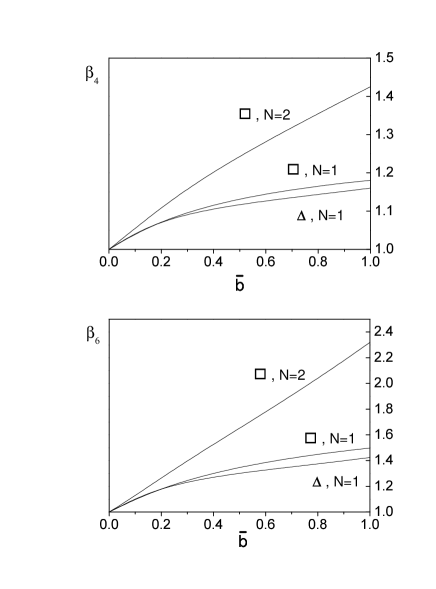
FIG. 1.: Structural factors $\beta_{4}^{(N)}=<\left|\psi\right|^{4}>/<\left|\psi\right|^{2}>^{2}$ and $\beta_{6}^{(N)}=<\left|\psi\right|^{6}>/<\left|\psi\right|^{2}>^{3}$ for triangle and square N-quanta vortex lattices as function of the average magnetic induction $\bar{b}$.

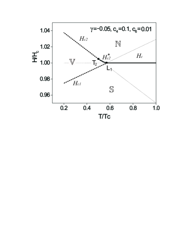
FIG. 2.: $H$-$T$ phase diagram of superconductor with $c_{4},c_{6}>0$ and with $\gamma$ slightly less then zero It includes normal (N), vortex (V) and Meissner superconducting (S) phases. Solid and dashed lines corresponds to the discontinuous and continuous transitions, dotted lines present the auxiliary critical fields. Magnetic field is measured in units of the temperature dependent critical field $H_{c}=H_{c}^{\prime}(T_{c}-T)$.

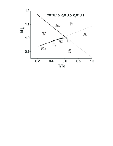
FIG. 3.: The same as Fig. 2 but for $c_{4}>0$, $0>c_{6}>-c_{4}/3$ when $\gamma$ is slightly less then zero.

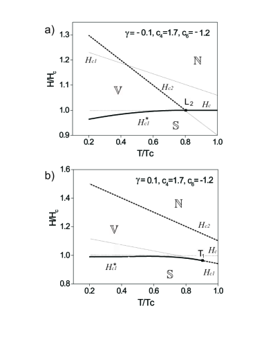
FIG. 4.: The same as Fig. 2 and Fig. 3 but for $c_{4}>0$, $-c_{4}/3>c_{6}$ when (a) $\gamma$ is slightly less then zero (a) and when $\gamma$ is slightly larger then zero (b).

REFERENCES

- [1] E. B. Bogomolnyi, Yad. Fiz. 24, 861 (1976) [Sov. J. Nucl. Phys. 24, 449 (1976)]; E. B. Bogomolnyi and A. I. Vainstein, Yad. Fiz. 23, 1111 (1976) [Sov. J. Nucl. Phys. 23, 588 (1976)]
- [2] L. Jacobs and C. Rebbi, Phys. Rev. B19, 4486 (1979)
- [3] E. Akkermans and K. Mallick cond-mat/0001219 (2000); E. Akkermans, D. M. Gangardt and K. Mallick cond-mat/0005542 (2000)
- [4] A. V. Efanov, Phys. Rev. B56, 7839 (1997)
- [5] A. A. Abrikosov, Zh. Eksp. Teor. Fiz. 32, 1442 (1957) [Sov. Phys. JETP 5, 1174 (1957)]
- [6] R. P. Hübener, Magnetic Flux Structures in Superconductors, Springer (1979)
- [7] E. H. Brandt and U. Essmann, Phys. Stat. Sol. (b) 144, 13 (1987)
- [8] D. Saint-James, G. Sarma and E. J. Thomas, Type II superconductivity, Pergamon (1969)
- [9] K. Maki, Physics, 1, 21 (1964); 1, 127 (1964)
- [10] Caroli C., Cyrot M. and De Gennes P. G., Sol. State. Comm. 4, 17 (1966)
- [11] K. Maki and T. Tsuzuki, Phys. Rev. A139, 868 (1965)
- [12] G. Eilenberger, Phys. Rev. 153, 584 (1967)
- [13] L. Tewordt, Z. Physik, 180, 385 (1964)
- [14] L. Tewordt, Phys. Rev. 135, A1745 (1965)
- [15] L. Neumann and L. Tewordt, Z. Physik 189, 55 (1966)
- [16] L. Tewordt, Z. Physik, 184, 319 (1965)
- [17] A. E. Jacobs, Phys. Rev. B4, 3016 (1971); B4, 3022 (1971); B4, 3029 (1971)
- [18] A. Hubert, Phys. Stat. Sol. (b) 53, 147 (1972)
- [19] S. Großmann and Ch. Wissel, Z. Physik 252, 74 (1972)
- [20] E. H. Brandt, Phys. Stat. Sol. (b) 77, 105 (1976)
- [21] Y. N. Ovchinnikov, Zh. Eksp. Teor. Fiz. 115, 726 (1999) [Sov. Phys. JETP 88, 398 (1999)]
- [22] T. McConville and B. Serin, Phys. Rev. A140, 1169 (1965)
- [23] T. McConville and B. Serin, Rev. Mod. Phys. 36, 112 (1964)
- [24] J. Schelten, H. Ullmaier and W. Schmatz, Phys. Stat. Sol. (b) 48, 619 (1971)
- [25] H. W. Weber, J. Schelten and G. Lippmann, Phys. Stat. Sol. (b) 57, 515 (1973)
- [26] J. Auer and H. Ullmaier, Phys. Rev. B7, 136 (1973)
- [27] T. Kinsel, E. A. Lynton and S. Serin, Rev. Mod. Phys. 36, 105 (1964)
- [28] U. Krägeloh, Phys. Stat. Sol. 42, 559 (1970)
- [29] H. Träuble and U. Essmann, Phys. Stat. Sol. 20, 95 (1967)
- [30] N. V. Sarma, Phil. Mag. 18, 171 (1968)
- [31] Partial Differential Equation Toolbox Users Guide, The MathWorks, Inc.(1996)