Abstract

The current status of experiments on the $d=2$ and $d=3$ random-exchange and random-field Ising models, as realized in dilute anisotropic antiferromagnets, is discussed. Two areas of current investigation are emphasized. For $d=3$, the large random field limit is being investigated and equilibrium critical behavior is being characterized at high magnetic concentrations.

1 Introduction

The Ising model is one of the most studied and basic models for phase transitions. In this article, the current status of experimental studies characterizing two classic models of second-order phase transitions in short-range interaction systems in the presence of quenched disorder, the random-exchange Ising model (REIM) and the random-field Ising model (RFIM), is presented. The discussion concentrates on experiments in dilute, insulating, anisotropic antiferromagnets, the systems that have yielded the best understood data for these two models. The REIM is realized in zero magnetic field and the RFIM with a field applied along the spin-ordering direction. The REIM is rather well characterized experimentally, theoretically and through computer simulations. The $d=2$ RFIM is fairly well characterized, although the scaling behavior of scattering near the destroyed phase transition is still being investigated. The understanding of the RFIM for $d=3$ is not as complete, though significant progress has been made in the past few years, and it is this model that will be the main focus of this short review. The early history of the $d=3$ RFIM was fraught with controversial interpretations of the data, a result of severe nonequilibrium effects. Nevertheless, some experimental groups realized from the start that underlying the observed, complicated behavior is a new kind of phase transition. Efforts to characterize the new critical behavior were thwarted by the severe nonequilibrium effects. These nonequilibrium effects have recently been overcome by going to sufficiently high magnetic concentration and a complete characterization of the universal $d=3$ RFIM critical behavior is possible and underway. The most recent static critical behavior will be compared to results from computer simulations and theory. In addition to these low-field behaviors, much has been learned about the high-field limit of the RFIM. An overview will be given of the phase diagram and the different behaviors observed.

Experiments have been performed on REIM and RFIM systems for more than two decades. Since the experiments performed some time ago have been reviewed previously[1], they will be included here only as needed to give a perspective on the current physical understanding of the models. Theory and simulation results will be included as needed for the interpretation of the experiments. Another classic model of ordering in the presence of disorder, the spin glass, will be covered in another review[2] in this Ising Colloquium and so will not be discussed here in detail, although some spin-glass-like behaviors do occur at low magnetic concentrations and at high magnetic fields.

Table 1 shows the most frequently measured static critical behaviors associated with a phase transition. We will make reference to the universal parameters defined in Table 1 as needed.

specific heat	$C=A^{\pm}|t|^{-\alpha}+B$
for $\alpha\rightarrow 0$	$C=A\ln|t|$
order parameter ($T<T_{c}$)	$M_{s}=M_{o}|t|^{\beta}$
fluctuation correlation length	$\xi=\xi_{o}^{\pm}|t|^{-\nu}=1/\kappa$
staggered susceptibility	$\chi_{s}=\chi_{o}^{\pm}|t|^{-\gamma}$
disconnected susceptibility	$\chi_{s}^{d}=\chi_{o}^{d\pm}|t|^{-\bar{\gamma}}$

Table 1: The asymptotic forms for commonly measured static critical behaviors. The superscript + (-) on the amplitudes signifies $T>T_{c}$ ($T<T_{c}$). The exponent values and the amplitude ratios are universal quantities that depend only on the general properties of the system.

2 Experiments on Pure $d=2$ and $d=3$ Anisotropic Antiferromagnets

Observations of asymptotic static critical behavior in the pure $d=2$ and $d=3$ Ising antiferromagnets are very well documented. The magnetic specific heat ($C_{m}$) critical behavior has been characterized using the optical linear birefringence techniques[3, 4] on the $d=2$ $\rm{Rb}_{2}\rm{CoF}_{4}$ system[5] and the $d=3$ $\rm{FeF}_{2}$ system[6]. The measured pure Ising critical exponents $\alpha$ and the amplitude ratios $A^{+}/A^{-}$ are in superb agreement with very many theoretical and simulation results. The birefringence technique is particularly useful and more accurate than pulsed specific heat techniques since it is insensitive to the large phonon contributions which are particularly difficult to handle for $d=2$.

The critical behavior of the staggered susceptibility and correlation length have been determined with neutron scattering for $\rm{K}_{2}\rm{CoF}_{4}$[7] for $d=2$ and in $\rm{FeF}_{2}$[8] for $d=3$. In general, the scattering line shapes for the pure and REIM systems away from the Bragg scattering point follow the scaling behavior of the spin-spin correlation function

$${\chi_{s}}(q)=A^{\pm}\kappa^{\eta-2}f(q/\kappa)\quad,$$ (1)

where $\gamma=\nu(2-\eta)$. For both $d=2$ and $d=3$, the scaling functions used in data analysis are approximate ones[9, 10] that differ significantly from the mean-field (MF) Lorentzian

$$f(q/\kappa)=\frac{1}{1+(q/\kappa)^{2}}\quad,$$ (2)

as can be seen in Fig. 1 where various scaling functions are compared. The deviation from the Lorentzian is more pronounced for $d=2$ and for $T<T_{c}(H)$ in both dimensions.

The order parameter critical behavior has been determined using neutron scattering[7] in the $d=2$ compounds. The Mössbauer technique[11] was used in the study of the $d=3$ system.

The results for the pure Ising model in $d=2$ and $d=3$ are summarized in Table 2. Note that the Rushbrooke scaling relation

$$2\beta+\gamma+\alpha\geq 2$$ (3)

is satisfied as an equality for both cases. Included in Table 2 are the results from a few theoretical and simulation studies. No attempt is made to review the vast literature on the pure Ising models.

Pure $d=2$	Experiment	Theory[12]
$\alpha$	$0.00\pm 0.01$[6]	$O(\log|t|)$
$A^{+}/A^{-}$	$1.01\pm 0.00$[6]	$1(\log|t|)$
$\beta$	$0.155\pm 0.02$[7]	$1/8$
$\nu$	$1.02\pm 0.05^{+}$[7]	$1$
	$1.12\pm 1.13^{-}$[7]
$\kappa^{+}/\kappa-$	$0.54\pm 0.06$[7]	$1/2$
$\gamma$	$1.82\pm 0.07$[7]	$7/4$
	$1.92\pm 0.20$[7]
$\chi^{+}/\chi^{-}$	$32.6\pm 3.7$[7]	$37.33$
Pure $d=3$	Experiment	Theory
$\alpha$	$0.11\pm 0.005$[13]	$0.1099\pm 0.0007$[14]
		$0.109\pm 0.004$[15]
$A^{+}/A^{-}$	$0.54\pm 0.02$[13]	$0.55$[16]
$\beta$	$0.325\pm 0.005$[11]	$0.32648\pm 0.00018$[14]
		$0.3258\pm 0.0014$[15]
$\nu$	$0.64\pm 0.01$[8]	$0.63002\pm 0.00023$[14]
		$0.6304\pm 0.0013$[15]
$\kappa^{+}/\kappa-$	$0.53\pm 0.01$[8]	$0.52$[16]
$\gamma$	$1.25\pm 0.02$[8]	$1.2371\pm 0.0004$[14]
		$1.2396\pm 0.0013$[15]
$\chi^{+}/\chi^{-}$	$4.6\pm 0.2$[8]	$4.8$[16]

Table 2: The pure $d=2$ and $d=3$ Ising static critical exponents obtained from experiments, theory and Monte Carlo simulations.

3 Random-Exchange Experiments in Dilute $d=2$ and $d=3$ Anisotropic Antiferromagnets

The REIM is realized in dilute, anisotropic insulating antiferromagnets when the site dilution does not result in strongly frustrated bonds (that would lead to spin-glass behavior). Random-exchange phase transitions are observed in $d=2$ and $d=3$ systems and these appear to be in good accord with theory and simulations.

The $d=2$ REIM $C_{m}$ critical behavior was observed using the birefringence technique[5] on the magnetically dilute antiferromagnet $\rm{Rb}_{2}\rm{Co}_{0.85}\rm{Mg}_{0.15}\rm{F}_{4}$. The approximately logarithmic divergence is compatible with theoretical predictions[17, 18]. The scattering critical behavior[19] of the compound $\rm{Rb}_{2}\rm{Co}_{x}\rm{Mg}_{1-x}\rm{F}_{4}$ was analyzed using approximate scattering line shapes[9, 10] developed for the pure $d=2$ Ising model. The successful analysis using these line shapes suggests that the correct line shape is close to the pure one. The static critical behavior of the $d=2$ Ising model is quite well characterized by experiments and theory as shown in Table 3.

$d=2$ Random	Experiment	Theory[20, 17]
Exchange	($H=0$)
$\alpha$	$\approx O(\log|t|)$[5]	$O(\log(\log 1/|t|))$
$A^{+}/A^{-}$	$0.95\pm 0.10$[6]	$1(\log|t|)$
$\beta$	$0.13\pm 0.02$[19]	$1/8$
$\nu$	$1.08\pm 0.06^{+}$[19]	$1$
	$1.58\pm 0.52^{-}$[19]
$\kappa^{+}/\kappa-$	$0.98\pm 0.02$[19]	$1/2$
$\gamma$	$1.75\pm 0.07$[19]	$7/4$
	$2.6\pm 0.6$[19]
$\chi^{+}/\chi^{-}$	$19.1\pm 5.0$[19]	37.33
$d=3$ Random	Experiment	Theory
Exchange	($H=0$)
$\alpha$	$-0.10\pm 0.02$[21]	$-0.051\pm 0.013$[22]
$A^{+}/A^{-}$	$1.55\pm 0.15$[23]	$-0.5$[24]
$\beta$	$0.350\pm 0.009$[25]	$0.3546\pm 0.0028$[22]
$\nu$	$0.69\pm 0.01$[26]	$0.6837\pm 0.0053$[22]
$\kappa^{+}/\kappa-$	$0.54\pm 0.06$[26]	$0.83$[24]
$\gamma$	$1.31\pm 0.03$[26]	$1.342\pm 0.010$[22]
$\chi^{+}/\chi^{-}$	$2.8\pm 0.2$[26]	$1.7$[24]

Table 3: The $d=2$ and $d=3$ REIM Ising static critical exponents obtained from experiments, simulations and theory.

The $d=3$ REIM is similarly well characterized with birefringence, neutron scattering and Mössbauer experiments employing $\rm{Fe}_{x}\rm{Zn}_{1-x}\rm{F}_{2}$ with the results shown in Table 3 along with some theoretical and simulation results with which they agree very well. The critical behavior of the specific heat of the $d=3$ REIM, measured with birefringence techniques[21], is shown in Fig. 2. Monte Carlo simulations[27] based on the $\rm{Fe}_{x}\rm{Zn}_{1-x}\rm{F}_{2}$ system are shown in Fig. 3. The birefringence technique yields a negative specific heat exponent $\alpha$ as predicted[28], consistent with a universality class different from the pure Ising model where $\alpha$ is positive. Note that, just as in the pure case, the birefringence technique is consistent with pulsed specific heat techniques, though the latter technique suffers from greater concentration gradient sensitivity[29] and the large phonon specific heat component. The critical behaviors of the staggered susceptibility and correlation length were determined from neutron scattering experiments[26]. The order parameter critical behavior was determined from Mössbauer studies[25]. The scattering line shape scaling functions are not known from theory and were therefore determined directly from the scattering data in neutron scattering experiments[30] using $\rm{Fe}_{0.93}\rm{Zn}_{0.07}\rm{F}_{2}$. The results shown in Fig. 1 clearly indicate that the scaling functions are fairly close to those of the pure $d=3$ case.

The REIM universal static critical parameters for $d=2$ and $d=3$ are shown in Table 3 along with theoretical and simulation results. In both dimensions the agreement is excellent. Note that the Rushbrooke scaling relation (Eq. 3) is satisfied as an equality for the REIM.

$d=3$ Random	$Fe_{x}Zn_{1-x}F_{2}$	Monte Carlo
Field	($H>0$)	& Exact Ground State
$\alpha$	$0.0\pm 0.02$[21]	$-0.5\pm 0.2$[31]
		$-0.55\pm 0.2$[32]
$\beta$	not measured[33]	$0.00\pm 0.05$[31]
		$0.02\pm 0.01$[32]
		$0.25\pm 0.03$[27]
$\nu$	$0.88\pm 0.05$	$1.1\pm 0.2$[31]
		$1.14\pm 0.10$[32]
$\gamma$	$1.58\pm 0.13$	$1.7\pm 0.2$[31]
		$1.5\pm 0.2$[32]
$\bar{\gamma}$	$2\gamma=3.16\pm 0.26$	$3.3\pm 0.6$[31]
		$3.4\pm 0.4$[32]

Table 4: The $d=3$ RFIM Ising static critical exponents obtained from experiments, simulations and theory.

4 The $d=3$ Magnetic Percolation Threshold Concentration

As the magnetic percolation threshold concentration, $x_{p}$, is approached from above in zero field, the equilibrium phase transition is expected to approach zero temperature. For a particular magnetic structure, $x_{p}$ depends on what interactions exist between the different neighboring spins. For example, for $\rm{Fe}_{x}\rm{Zn}_{1-x}\rm{F}_{2}$, $x_{p}=0.245$ provided only the dominant interaction between the body-center and corner spins is considered[34]. Except very close to $x_{p}$, the much smaller interactions can be ignored. Close to $x_{p}$, however, the smaller interactions may drastically affect the behavior and even prevent ordering above $x_{p}$ when they frustrate the dominate interaction. Both the extremely slow dynamics near percolation[35] and the sensitivity to tiny frustrating interactions[36] can cause the system to exhibit spin-glass-like behavior.

A good deal of effort has focused on the properties of the system $\rm{Fe}_{x}\rm{Zn}_{1-x}\rm{F}_{2}$ for $x$ near $x_{p}$. This system has a small frustrating interaction[37]. The spin-glass-like properties were first elucidated in experiments by Montenegro, et al.[38, 39, 40, 41, 42, 43]. For $H>0$ and $x=x_{p}$, there exists a boundary that resembles a de Almeida-Thouless boundary with curvature $T-T_{o}\sim H^{2/\phi}$ where $\phi=3.4$, a typical spin-glass value. It was shown with neutron scattering[44] that there is no antiferromagnetic long-range ordering below this boundary. Much of the behavior is very reminiscent of a canonical spin glass. The detailed behavior of this sample has been studied experimentally[38, 45] and extensively modeled in local mean-field[46, 47] and Monte Carlo simulations[48].

5 $d=2$ Random-Field Behavior

Scaling arguments for Zeeman and domain wall energies by Imry and Ma[49] as well as considerations by Binder[50] leave little doubt that the $d=2$ Ising transition is destroyed by the introduction of arbitrarily small random fields. Birefringence[5] and neutron Bragg scattering[51] experiments bear this out; no sharp phase transition is observed in equilibrium, though the rounded transition exhibits the expected scaling behavior. The equilibrium region is separated from a lower temperature region of strong hysteresis observed in the difference between data obtained upon heating after cooling in zero field to low temperatures and then applying the field (ZFC) and upon simply cooling the sample in the field (FC). The boundary separating these regions is time-scale dependent[52]. The domain dynamics induced with the application of a magnetic field as well as those remaining after the field is removed at low temperatures have been studied experimentally[53, 54] and theoretically[55].

6 $d=3$ RFIM behavior for $x_{p}<x<x_{e}$ at low fields.

The behavior for concentrations between $x_{p}$ and the percolation threshold concentration for vacancies, $x_{e}=1-x_{p}$, with a relatively small applied field occupied the bulk of early experimental efforts[1]. Much of the controversy over interpretations of experimental data involved this region of concentration and fields. As a result of the equivalence[56, 57] of the dilute anisotropic antiferromagnet in small fields and the random-field ferromagnet often studied theoretically, it was believed that concentrations near $x=0.5$ would yield strong random-field effects in reasonably small fields and would be the best realizations of the $d=3$ RFIM for phase transition studies. At the time of the first experiments[58, 59, 60, 61], it was generally believed, based on many theoretical arguments, that no phase transition would be observed. Indeed, early neutron scattering FC experiments, by Yoshizawa, et al.[61], seemed to bear this out. In particular, a resolution-limited Gaussian Bragg peak does not occur upon FC, although subsequent experiments[54] show that the samples retain long-range order below the phase boundary if ZFC. In contrast, the first $C_{m}$ studies[60, 62] yielded compelling evidence for a fundamentally new phase transition governing the behavior. The phase boundary $T-T_{c}(H)\sim H^{2/\phi}$ behaves as predicted[63] with $\phi=1.42\pm 0.03$ for random-exchange to random-field crossover[64].

Despite the sharp $C_{m}$ peak, many have argued against it as evidence of the existence of a phase transition. The most recent of these is the “trompe l’oeil transition” phenomenological model[65]. Among the assumptions of this model are that the birefringence and $C_{m}$ experiments do not yield the same behavior, the uniform magnetization is reflected by the square of the staggered magnetization, and conventional scaling is inoperative. This phenomenological model was shown to be inconsistent[66] when all available data are considered. In contrast, more proven and conventional techniques of analyzing the experimental data, as described in this review, have been very fruitful in providing consistent results in a meaningful scaling context.

It is clear that the phase transition underlying the behavior is obscured by nonequilibrium behavior below the boundary, $T_{eq}(H)$, lying just above the phase transition and scaling in the same manner, albeit with a slightly larger amplitude[67]. The equilibrium behavior above $T_{eq}(H)$ can be used to extrapolate the scattering data to the obscured phase transition boundary. When done carefully, the boundary determined in this way coincides with that determined via $C_{m}$ experiments, which are much less sensitive to the non-equilibrium behavior that distorts the neutron scattering data. For a long time, the nonequilibrium experiments represented the best random-field results available. One of the particularly interesting predictions[31] of the change in the critical behavior induced by the random fields is that the order parameter critical exponent $\beta$ should decrease from $0.35$ to a value near zero. This can only be measured below $T_{c}(H)$, i.e. in the nonequilibrium region, so it was not clear what would be observed. Experiments on thin films were made[68] for $x=0.52$, well below $x_{e}\approx 0.76$. Not surprisingly, the results were peculiar. The curvature of the Bragg intensity versus $T$ was such that it would require $\beta>>0.5$, which is hard to justify theoretically. Magnetic x-ray scattering data showed similar behavior near surfaces in bulk samples, though they were interpreted under the “trompe l’oeil” phenomenology and the Bragg scattering was not separated from the fluctuation scattering[65]. For some years it appeared that the problems of metastability below $T_{eq}(H)$ could not be avoided, i.e. that they were intrinsic to the random-field behavior as realized in dilute antiferromagnets. However, insight into the origins of the metastable domains finally led to experiments[30] at high magnetic concentration as a way to avoid the nonequilibrium behavior, as discussed later.

The metastable domains formed upon FC are themselves quite interesting and their dynamics were studied in some detail both experimentally[69, 70, 71, 62, 72] and through simulations[73, 74, 75].

7 RFIM behavior for $x_{p}<x<x_{e}$ at high fields.

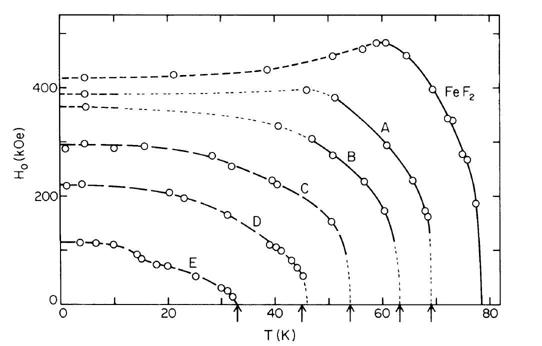
Figure 4: The $H-T$ phase diagram for $Fe_{x}Zn_{1-x}F_{2}$ measured in pulsed magnetic fields. The concentrations for the alphabetic labels are the same as in Fig. 5.

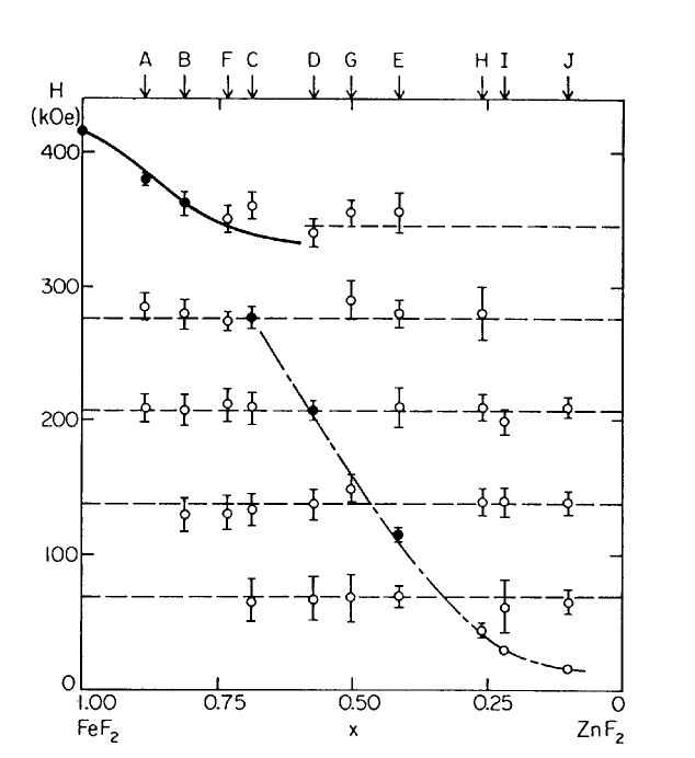
Figure 5: Low temperature spin flips and phase boundary for $Fe_{x}Zn_{1-x}F_{2}$ as a function of $x$. Note that the phase boundary behavior is quite different for $x<x_{e}$ and $x>x_{e}$.

The general phase diagram features, shown in Fig. 4 for the RFIM at high fields were investigated in pioneering pulsed-field magnetization measurements[76] in $\rm{Fe}_{x}\rm{Zn}_{1-x}\rm{F}_{2}$. Low temperature single spin flips and the phase boundary are shown in Fig. 5 and, interestingly, the behavior of the upper phase boundary appears to be different for $x<x_{e}$ and $x>x_{e}$. This is consistent with the differentiation of the behaviors observed in neutron scattering experiments above and below $x_{e}$.

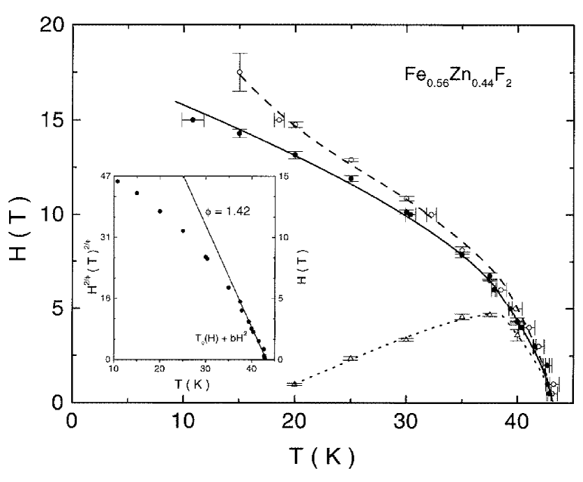
Figure 6: The $H-T$ phase diagram for $x=0.56$ showing the upper equilibrium boundary, the phase boundary and a lower equilibrium boundary.

In recent years, it has become clear that weak RFIM (small applied field) and strong RFIM regimes exist for $x_{p}<x<x_{e}$. The $\rm{Fe}_{0.31}\rm{Zn}_{0.69}\rm{F}_{2}$ system exhibits[77] typical low-field behavior for $H<1.5$ T, with $T_{N}-T_{c}(H)$ and $T_{N}-T_{eq}(H)$ scaling as $H^{2/\phi}$ with $\phi\approx 1.4$. At larger fields, however, the curvature for $T_{N}-T_{eq}(H)$ changes to $\phi\approx 3.4$, a value close to that observed in spin glasses. Some of these features were suggested qualitatively[78, 79]. While the lower region has been shown to have antiferromagnetic long-range order upon ZFC[80], no long-range antiferromagnetic order is observed at the higher fields below $T_{eq}(H)$. Instead, spin-glass-like behavior is observed. This is clearly the same type of behavior observed for all fields at the percolation threshold concentration[81]. The same type of distinctive low and high field behaviors have been observed for $x$ as large as $0.60$. The two regions are separated by an equilibrium boundary[82, 83], as observed for $x=0.56$ (Fig. 6) and $0.60$, and it appears to decrease towards the $H=0$ boundary at finite temperature well below $T_{c}(H)$ and approach the phase transition line at finite field, a point separating the sharp transition observed at low field and the more glassy transition at higher fields. This also is consistent[84] with specific heat peaks that are very sharp at low fields and quite rounded at high fields[85, 65].

The distinction between high- and low-field behavior behavior is observed as well in ac susceptibility experiments. At low fields, there exists a single peak which seems to be associated with extremely slow dynamics, either from activated dynamics or at least power-law behavior with a very large dynamic exponent[86, 87]. There is little hysteresis between the ZFC and FC procedures at low $H$. At larger fields the peak splits in the ZFC procedure only, with a sharp peak at slightly lower temperatures than the broader peak[88, 84]. This splitting appears to be associated with the upper region of the phase diagram corresponding to the spin-glass-like behavior[84]. These effects have not been investigated for $x>x_{p}$. The high field region for these concentrations is still an open area for research.

8 $d=3$ RFIM Equilibrium Critical Behavior for $x>x_{e}$

It was, of course, realized very early that the metastable domain walls at low magnetic concentrations took advantage of vacancies. What was not fully appreciated was that the Imry-Ma domain wall energy argument[49] is not applicable when domain walls can to a great extent pass through vacancies, avoiding the energy cost of breaking magnetic bonds. With sufficient vacancies, i.e. for $x<x_{e}$, domain walls can take advantage of vacancies to such an extent that the domain wall energy can be insignificant. Interestingly, every experiment that could have detected low temperature hysteresis, particularly neutron scattering and capacitance[67] experiments, was done for $x\leq 0.72$, which is below $x_{e}=0.76$. Higher concentrations were avoided since the generated random fields are small, resulting in relatively very narrow asymptotic random-field critical regions around $T_{c}(H)$. Nevertheless, concentrations well above $x_{e}$ are necessary to study the equilibrium critical behavior and require high magnetic fields and very fine temperature resolution.

Figure 2 shows the specific heat data for $\rm{Fe}_{0.93}\rm{Zn}_{0.07}\rm{F}_{2}$, measured with optical linear birefringence. The specific heat was also measured to demonstrate that, in agreement with theory[3] and contrary to the so-called ‘trompe l’oeil’ phenomenology[65], the data from the both techniques yield the same critical parameters. An important advantage of the birefringence technique is its relative insensitivity to the concentration gradients that tend to smear the transition[29]. Interestingly, the critical behavior appears to be very similar to that of lower concentrations where metastable domains dominate the scattering behavior. The specific heat was studied using Monte Carlo simulations[27] based on the $\rm{Fe}_{0.93}\rm{Zn}_{0.07}\rm{F}_{2}$ system and the results are shown in Fig. 3. Although the simulations are not of sufficient resolution to extract the critical exponent, the similarities in the shapes of both the REIM and RFIM indicate the same qualitative change from the asymmetric cusp at $H=0$ to the nearly symmetric peaks at $H>0$. This result, however, is not seen in all MC simulations[31].

The neutron scattering experiments on $\rm{Fe}_{0.93}\rm{Zn}_{0.07}\rm{F}_{2}$ show no hysteresis below the phase transition, in stark contrast with samples with $x<x_{e}$. There is no evidence that domains form upon ZFC or FC in this concentration range and the line shapes are independent of the thermal cycling procedure, implying equilibrium conditions.

Neutron scattering experiments on this sample were difficult to analyze since the RFIM line shape is not known from theory. In general, two different scaling functions are involved with the form

$${\chi_{s}}(q)=A^{\pm}\kappa^{\eta-2}f(q/\kappa)+B^{\pm}\kappa^{\bar{\eta}-4}g(q/\kappa)\quad.$$ (4)

with two independent sets of critical behavior exponents. However, simulations[22] and high temperature series expansions[89] strongly suggest a simpler scenario. The predictions are that the exponents are simply related, $\bar{\eta}$ being twice $\eta$, and the new scaling function $g(q/\kappa)$ is, to a good approximation, the square of $f(q/\kappa)$.

Not only were the universal RFIM critical parameters obtained in this experimental study, but the scaling analysis yielded the spin-spin correlation scaling function $f(q/\kappa)$. This scaling function is compared to several other known spin-spin correlation scaling functions in Fig. 1. Note that the $d=3$ RFIM one seems the furthest away from the MF Lorentzian of all the examples for $T>T_{c}(H)$, whereas for $T>T_{c}(H)$ the pure $d=2$ case is further than the $d=3$ RFIM, though both are very far from MF behavior.

The critical parameters for the RFIM with $x>x_{e}$ are shown in Table 4. Certainly more effort is needed to complete the experimental entries and to find reconciliation between the simulation and experimental results. Note that some sets of exponents from the simulations violate[32] the Rushbrooke scaling relation in Eq. 3.

9 The Vacancy Percolation Threshold Concentration

The regions of low temperature nonequilibrium behavior and equilibrium behavior have been shown to be separated at relatively small $H$ by a nearly vertical sharp boundary at $x\approx x_{e}=0.755$ in $\rm{Fe}_{x}\rm{Zn}_{1-x}\rm{F}_{2}$ using Monte Carlo studies[90]. Figure 7 shows simulations on lattices of size $2\times L^{3}$ with $L=64$ modeled closely after $\rm{Fe}_{x}\rm{Zn}_{1-x}\rm{F}_{2}$. Hysteresis is observed upon FC and ZFC for $x<x_{e}$ but not above. The hysteresis for $x<x_{e}$ increases for larger lattices or slower thermal cycling, showing that it is not simply an artifact of the simulations not being run long enough. The concentration dividing equilibrium and nonequilibrium behavior is very close to or equal to the vacancy percolation threshold concentration $x_{e}=0.755$. Apparently, the percolation vacancy structure facilitates the formation of domain walls.

To further investigate this boundary, recent experiments have been done[91] on a sample with $x=0.76$, just above $x_{e}$. No evidence of domains has been observed for small $H$. Since earlier experiments[67] for $x=0.72$ in $\rm{Fe}_{x}\rm{Zn}_{1-x}\rm{F}_{2}$ gave clear evidence for domain formation, including a reversal of the Bragg intensity curvature just below $T_{c}(H)$ upon ZFC, the boundary must be $0.72<x_{e}<0.76$, in agreement with the MC simulations. There have been no theoretical studies reported explaining the existence or nature of this boundary.

10 The Current Situation and Outlook

The recent measurement of the equilibrium critical behavior in the random-field Ising model has side-stepped the great difficulties encountered in the interpretation of data below the transition that are obfuscated by nonequilibrium phenomena in many studies at lower concentrations. Certainly, there is wide agreement that a phase transition exists. Although experiments for $x>x_{e}$ are much more difficult since the random-field region is very narrow, they are being done. Interestingly, the experimental results are not in agreement with much of the theory and simulation results, unlike the REIM and pure Ising model. A reliable characterization of some aspects of the $d=3$ RFIM universality class behavior remains to be completed. The phase diagram of $\rm{Fe}_{x}\rm{Zn}_{1-x}\rm{F}_{2}$ has proven to be quite rich in detail. An important area of the phase diagram for which a good understanding is being developed is the large random field limit for $x_{p}<x<x_{e}$. With the the progress being made along these two lines of inquiry, a rather complete experimental characterization of the RFIM in dilute antiferromagnets seems near at hand.

Recent work has been supported by Department of Energy Grant No. DE-FG03-87ER45324.

Figure 1: A comparison of the logarithm of the scaling functions $f(q/\kappa)$ versus $q/\kappa$ for different models (See Eq. 1). The pure cases are from approximate expressions from numerical studies[9, 10]. The REIM and RFIM are determined from the experiments. Note that the corrections to the MF equation are largest below the transition and are very significant for the pure $d=2$ and random-field $d=3$ cases.

Figure 2: $C_{m}$ vs. $T$ for $\rm Fe_{0.93}Zn_{0.07}F_{2}$ at $H=7$ T as determined using the birefringence technique. The inset shows the FC data. There appears to be a tiny hysteresis very close to the transition, perhaps a consequence of random-field activated dynamics.

Figure 3: $C_{m}$ vs. $T$ from Monte Carlo simulations modeled after the $\rm Fe_{0.8}Zn_{0.2}F_{2}$ system. The simularity with the data is striking, though not all Monte Carlo simulations yield a sharp peak in $C_{m}$.

Figure 7: Monte Carlo simulation data for the staggered magnetization versus $T$ for magnetic concentrations $0.5$, $0.6$, $0.7$ and $0.8$. The ZFC and FC procedures exhibit hysteresis for the lower concentrations, which only gets worse for slower runs or larger lattices. No hysteresis is observed for the higher concentrations.

References

- [1] D. P. Belanger and A. P. Young, J. Mag. Mag. Mater. 100, 272 (1991); D. P. Belanger, in “Spin Glasses and Random Fields”, edited by A. P. Young, (World Scientific, Singapore, 1998), p.251; T. Nattermann, in “Spin Glasses and Random Fields”, edited by A. P. Young, (World Scientific, Singapore, 1998), p.277.
- [2] P. Nordblad, Ising Centennial Colloquium, 2000.
- [3] J. Ferré and G. A. Gehring, Rep. Prog. Phys. 47, 513 (1984).
- [4] D. P. Belanger, A. R. King and V. Jaccarino, Phys. Rev. B 29, 2636 (1984).
- [5] I. B. Ferreira, A. R. King, V. Jaccarino, J. L. Cardy and H. J. Guggenheim, Phys. Rev. B 28, 5192 (1983).
- [6] P. Nordblad, D. P. Belanger, A. R. King, V. Jaccarino, and H. Ikeda, Phys. Rev. B 28, 278 (1983).
- [7] R. A. Cowley, M. Hagen and D. P. Belanger, J. Phys. C 17, 3763 (1984).
- [8] D. P. Belanger and H. Yoshizawa, Phys. Rev. B 35, 4823 (1987).
- [9] H. B. Tarko and M. E. Fisher, Phys. Rev. B 11, 1217 (1975).
- [10] M. E. Fisher and R. J. Burford, Phys. Rev. 156, 583 (1967).
- [11] G. K. Wertheim and D. N. E. Buchanan, Phys. Rev. 161 478, (1967).
- [12] L. Onsager, Phys. Rev. 65, 117 (1944).
- [13] D. P. Belanger, P. Nordblad, A. R. King, V. Jaccarino, L. Lundgren and O. Beckman, J. Magn. Magn. Mater. 31-34, 1095 (1983).
- [14] M. Campostrini, A. Pelissetto, P. Rossi and E. Vicari, cond-mat/9905078 (1999).
- [15] R. Guida and J. Zinn-Justin, J. Phys. A 31, 8103 (1998).
- [16] E. Brezin, J. C. LeGuillou and J. Zinn-Justin, Phys. Lett. 47A, 285 (1974).
- [17] E. S. Sorensen, cond-mat/0006233 (2000).
- [18] R. Folk, Yu. Holovatch and T. Yavors’kii, Phys. Rev. B 61, 15114 (2000).
- [19] M. Hagen, R. A. Cowley, R. M. Nicklow and H. I. Ikeda, Phys. Rev. B 36, 401 (1987).
- [20] V. S. Dotsenko and V. S. Dotsenko, J. Phys. C 15, 495 (1983); J. Phys. C 15, L557 (1983).
- [21] Z. Slanič and D. P. Belanger, J. Magn. Magn. Mater. 186, 65 (1998).
- [22] H. G. Ballesteros, L. A. Fernández, V. Martín-Mayor, A. M. Sudupe, G. Parisi, and J. J. Ruiz-Lorenzo, Phys. Rev. B 58, 2740 (1998); also see A. Pelissetto and E. Vicari, cond-mat/0002402 (2000) and D. V. Pakhnin and A. I. Sokolov, cond-mat/9912071 (1999).
- [23] J. Wang and D. P. Belanger, unpublished.
- [24] S. A. Newlove, J. Phys. C 16, L423 (1983).
- [25] N. Rosov, A. Kleinhammes, P. Lidbjork, C. Hohenemser and M. Eibschutz, Phys. Rev. B 37, 3265 (1988).
- [26] D. P. Belanger, A. R. King, and V. Jaccarino, Phys. Rev. B 34, 452 (1986).
- [27] W. C. Barber and D. P. Belanger, ICM2000.
- [28] A. B. Harris, J. Phys. C 7, 1671 (1974).
- [29] D.P. Belanger, A.R. King, I.B. Ferreira, and V. Jaccarino, Phys. Rev. B 37, 226 (1987).
- [30] Z. Slanič , D. P. Belanger and J. A. Fernandez-Baca, Phys. Rev. Lett. 82, 426 (1999).
- [31] H. Rieger, Phys. Rev. B 52, 6659 (1995); H. Rieger and A. P. Young, J. Phys. A 26, 5279 (1993); J. Machta, M. E. J. Newman and L. B. Chayes, cond-mat/0006267 (2000).
- [32] U. Nowak, K. D. Usadel and J. Esser, Physica A 250, 1 (1998).
- [33] The only measurement is using the dilation technique at lower concentration where the system is not in equilibrium by C. A. Ramos, A. R. King, V. Jaccarino and S. M. Rezende, J. de Phys. 49, C8-1241 (1988).
- [34] M. F. Sykes and J. W. Essam, Phys. Rev. 133, A310 (1964).
- [35] C. L. Henley, Phys. Rev. Lett. 54, 2030 (1985).
- [36] B. W. Southern, A. P. Young and P. Pfeuty, J. Phys. C 12, 683 (1979).
- [37] W. C. Barber and D. P. Belanger, Phys. Rev. B 61, 8960 (2000).
- [38] S. M. Rezende, F. C. Montenegro, M. D. Coutinho-Filho, C. C. Becerra and A. Paduan-Filho, J. de Phys. C8, 1267 (1988).
- [39] F. C. Montenegro, M. D. Coutinho-Filho and S. M. Rezende, Europhys. Lett. 8, 382 (1989).
- [40] F. C. Montenegro, J. C. O. de Jesus, F. L. A. Machado, E. Montarroyos, and S. M. Rezende, J. Magn. Magn. Mater. 104-107, 277 (1992).
- [41] F. C. Montenegro, U. A. Leitão, M. D. Coutinho-Filho and S. M. Rezende, J. Appl. Phys. 67, 5243 (1990).
- [42] J. H. de Araujo, J. B. M. da Cunha, A. Vasquez, L. Amaral, J. T. Moro, F. C. Montenegro, S. M. Rezende and M. D. Coutinho-Filho, Rev. Brasil. de Fisica 21, 115 (1991).
- [43] F. C. Montenegro, S. M. Rezende and M. D. Coutinho-Filho, J. Appl. Phys. 63, 3755 (1988).
- [44] D. P. Belanger and H. Yoshizawa Phys. Rev. B 47, 5051 (1993).
- [45] K. Jonason , C. Djurberg , P. Nordblad and D. P. Belanger Phys. Rev. B 56, 5404 (1997).
- [46] E. P. Raposo, M. D. Coutinho-Filho and F. C. Montenegro, Europhys. Lett. 29, 507 (1995); J. Magn. Magn. 154, L155 (1996).
- [47] E. P. Raposo and M. D. Coutinho-Filho, Phys. Rev. B 57, 3495 (1998).
- [48] P. Barbosa, E. P. Raposo and M. D. Coutinho-Filho, J. Appl. Phys. 87, 6531 (2000).
- [49] Y. Imry and S. K. Ma, Phys. Rev. Lett. 35, 1399 (1975).
- [50] K. Binder, Z. Phys. B 50, 343 (1983); Phys. Rev. B 29, 5184 (1984).
- [51] D. P. Belanger, A. R. King and V. Jaccarino, Phys. Rev. Lett. 54, 577 (1985).
- [52] A. R. King, V. Jaccarino, M. Motokawa, K. Sugiyama and M. Date, J. Appl. Phys. 57, 3297 (1985).
- [53] W. Kleemann , Ch. Jakobs , Ch. Binek and D. P. Belanger, J. Magn. Magn. Mater. 177, 209 (1998).
- [54] D. P. Belanger, A. R. King and V. Jaccarino, Phys. Rev. B 31, 4538 (1985).
- [55] M. Staats, U. Nowak and K. D. Usadel, J. Magn. Magn. Mat. 177-181, 85 (1998).
- [56] J. L. Cardy, Phy. Rev. B 29, 505 (1984).
- [57] S. Fishman and A. Aharony, J. Phys. C 12, L729 (1979).
- [58] H. Rohrer, J. Appl. Phys. 52, 1708 (1981).
- [59] D. P. Belanger, A. R. King and V. Jaccarino, J. Appl. Phys. 53, 2702 (1982); Phys. Rev. Lett. 48, 1050 (1982).
- [60] D. P. Belanger, A. R. King, V. Jaccarino and J. L. Cardy, Phys. Rev. B 28, 2522 (1983).
- [61] H. Yoshizawa, R. A. Cowley, G. Shirane, R. J. Birgeneau, H. J. Guggenheim and H. Ikeda, Phys. Rev. Lett. 48, 438 (1982).
- [62] U. A. Leitão and W. Kleemann, Phys. Rev. B 29, 505 (1984); Phys. Rev. B 35, 8696 (1987).
- [63] A. Aharony, Europhys. Lett. 1, 617 (1986).
- [64] I. B. Ferreira, A. R. King, V. Jaccarino, Phys. Rev. B 43, 10797 (1991); J. Appl. Phys. 69, 5246 (1991).
- [65] R. J. Birgeneau, Q. Feng, Q. J. Harris, J. P. Hill, A. P. Ramirez, T. R. Thurston, Phys. Rev. Lett. 75, 1198 (1995); Phys. Rev. Lett. 77, 2342 (1996).
- [66] D. P. Belanger, W. Kleemann and F. C. Montenegro , Phys. Rev. Lett. 77, 2341 (1996).
- [67] A. R. King, V. Jaccarino, D. P. Belanger and S. M. Rezende, Phys. Rev. B 32, 503 (1985).
- [68] D. P. Belanger, J. Wang, Z. Slanič, S-J. Han, R. M. Nicklow, M. Lui, C. A. Ramos and D. Lederman, Phys. Rev. B 54, 3420 (1996).
- [69] M. Lederman, J. V. Selinger, R. Bruinsma, J. Hamman and R. Orbach, Phys. Rev. Lett. 68, 2086 (1992).
- [70] U. A. Leitão, W. Kleemann and I. B. Ferreira, Phys. Rev. B 38, 4765 (1988).
- [71] P. Pollak, W. Kleemann and D. P. Belanger, Phys. Rev. B 38, 4773 (1988).
- [72] J. Mattsson, C. Djurburg and P. Nordblad, Phys. Rev. B 61, 11274 (2000).
- [73] U. Nowak and K. D. Usadel, Phys. Rev. B 44, 7426 (1991); Phys. Rev. B 46, 8329 (1992); Phys. Rev. B 43, 851 (1991).
- [74] S-J. Han and D. P. Belanger, Phys. Rev. B 46, 2926 (1992).
- [75] S-J. Han, D. P. Belanger, W. Kleemann and U. Nowak, Phys. Rev. B 45, 9728 (1992).
- [76] A. R. King, V. Jaccarino, T. Sakakibara, M. Motokawa and M. Date, J. Magn. Magn. Mat. 31-34, 1119 (1983); Phys. Rev. Lett. 47, 117 (1981).
- [77] F. C. Montenegro, A. R. King, V. Jaccarino, S.-J. Han and D. P. Belanger, Phys. Rev. B 44, 2155 (1991).
- [78] C. M. Soukoulis, G. S. Grest, C. Ro and K. Levin, J. Appl. Phys. 57, 3300 (1985).
- [79] J. R. L. de Almeida and R. Bruinsma, Phys. Rev. B 35, 7267 (1987).
- [80] D. P. Belanger, Wm. Murray, F. C. Montenegro, A. R. King and V. Jaccarino, Phys. Rev. B 44, 2161 (1991).
- [81] K. Jonason, P. Nordblad and F.C. Montenegro, unpublished.
- [82] F. C. Montenegro, K. A. Lima, M. S. Torikachvili and A. H. Lacerda, J. Magn. Magn. Mater. 177 - 181, 145 (1998); Ising Centennial Colloquium.
- [83] F. C. Montenegro, K. A. Lima, M. S. Torikachvili and A. H. Lacerda, in: Proceedings of the Fourth Latin American Workshop on Magnetism, Magnetic Materials and their Applications, F.P. Missell (Ed.), Materials Science Forum, 302-303, 371 (1999).
- [84] A. Rosales-Rivera, J. M. Ferreira and F. C. Montenegro, Europhys. Lett. 50, 264 (2000); ICM2000 proceedings.
- [85] J. Satooka, H. Aruga Katori, A. Tobo and K. Katsumata, Phys. Rev. Lett. 81, 709 (1988).
- [86] A. R. King, J. A. Mydosh and V. Jaccarino, Phys. Rev. Lett. 56, 2525 (1986).
- [87] A. E. Nash, A. R. King and V. Jaccarino, Phys. Rev. B 43, 1272 (1991).
- [88] Ch. Binek, S. Kuttler and W. Kleemann, Phys. Rev. Lett. 75, 2412 (1995).
- [89] M. Gofman, J. Adler, A. Aharony, A. B. Harris and M. Schwartz, Phys. Rev. B 53, 6362 (1996).
- [90] W. C. Barber and D. P. Belanger, J. Appl. Phys. 87, 7049 (2000).
- [91] W. C. Barber, F. Ye, D. P. Belanger and J. A. Fernandez-Baca, unpublished.