Elastic moduli of model random three-dimensional closed-cell cellular solids

Abstract

Most cellular solids are random materials, while practically all theoretical results are for periodic models. To be able to generate theoretical results for random models, the finite element method (FEM) was used to study the elastic properties of solids with a closed-cell cellular structure. We have computed the density ($\rho$) and microstructure dependence of the Young’s modulus ($E$) and Poisson’s ratio (PR) for several different isotropic random models based on Voronoi tessellations and level-cut Gaussian random fields. The effect of partially open cells is also considered. The results, which are best described by a power law $E\propto\rho^{n}$ ($1<n<2$), show the influence of randomness and isotropy on the properties of closed-cell cellular materials, and are found to be in good agreement with experimental data.

Keywords: 1. Foams, 2. Mechanical properties: elastic, 3. Micro-structure

1 Introduction

Manufactured cellular materials have been developed for a range of applications [2] (e.g., insulation, light-weight reinforcement), and their natural counterparts (e.g. wood) have a cellular structure that optimizes performance for their particular requirements. The useful properties of cellular solids depend on the material from which they are made, their relative density, and their internal geometrical structure. It is important to link the physical properties of cellular solids to their density and complex microstructure, in order to understand how such properties can be optimized for a given application. Many studies have focussed on the elastic response of periodic materials. Equally important is the effect of disorder (e.g., isotropy), and the interaction between cells on a mesoscopic scale, as most real cellular solids are not periodic. In this paper we study model isotropic cellular solids at scales ($\approx$ 100 cells) where these effects can be probed.

At low densities, experimental results indicate that the Young’s modulus ($E$) of cellular solids is related to their density ($\rho$) through the relation [2]:

$$\frac{E}{E_{s}}=C\left(\frac{\rho}{\rho_{s}}\right)^{n}=Cp^{n}$$ (1)

where $E_{s}$ and $\rho_{s}$ are the Young’s modulus and density of the solid skeleton and $p=\rho/\rho_{s}$ is the reduced density. The constants $C$ and $n$ depend on the microstructure of the solid material. The value of $n$ generally lies in the range $1<n<4$, giving a wide range of properties at a given density. For closed-cell foams, experimental studies indicate that $1<n<2$. The complex dependence of $C$ and $n$ on microstructure is not well understood, and this remains a crucial problem in the ability to predict and optimize the elastic properties of cellular solids. At the local or cellular scale, important variables include the cell character (e.g. open or closed), the geometrical arrangement of the cell elements (e.g. angle of intersection), and the shape of the cell walls (e.g. curvature). At a larger scale, the geometrical arrangement of the cells is also crucial. The values of both $C$ and $n$ will depend on whether the material is periodic or disordered.

Analysis of simple models shows that three basic mechanisms of deformation are important for closed-cellular solids. If the cell walls are much thinner than the cell edges, the deformation is governed by edge-bending. In this case, $E$ varies quadratically with density ($n=2$), and can be described by results for open cellular solids [2]. If cell-wall bending is the mechanism of deformation, Gibson and Ashby [3] have shown that $E$ should vary cubicly ($n=3$) with density. However, the fact that $1<n<2$ indicates that cell-wall stretching ($n=1$) is actually the dominant behaviour [4, 2].

The “tetrakaidecahedral” foam model, in particular, has been the subject of many recent studies [5, 6, 7, 8, 9]. The cells of the model uniformly partition space, and are defined by truncating the corners of a cube giving eight hexagonal and six square faces (Fig. 1). The foam has a relatively low anisotropy [6] ($E$ varies by less than 10 % with direction of loading), and is thought to be a good model of isotropic cellular solids. In all cases, $E$ was found to decrease linearly with density ($n=1$). However, real materials exhibit a larger dependence of $E$ on density ($n>1$), indicating that periodic models do not capture salient features of foam microstructure. It is likely that the random disorder is responsible, and it is important to study its influence on the properties of cellular solids.

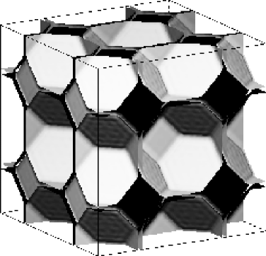
Figure 1: The tetrakaidecahedral model. The model corresponds to the Voronoi tessellation of a body-centered cubic lattice.

There have been several recent studies of the effect of disorder in cellular solids. For two-dimensional models, variation in cell-shape leads to a variation of 4 % to 9 % in elastic properties [10], while deletion of 5 % of cell struts decreased the modulus by 35 % [11]. Similar effects of ‘imperfections’ were seen in spring lattices, which have some similarities to foams [12]. In three-dimensions, Grenestedt [7] showed that disorder decreased the Young’s modulus of the tetrakaidecahedral foam (with 16 cells) by 10 %. However, only the pre-factor of Eq. (1) was affected; the scaling exponent remained constant ($n=1$). Grenestedt [13] has also estimated the effect of “wavy-imperfections” on the stiffness of a cube with closed cell walls. If the wave-amplitude was five times the cell-wall thickness, the stiffness decreased by 40 % compared to the case of flat faces.

From the foregoing discussion it is clear that more complex, three-dimensional random models are necessary to improve predictions for cellular solids [14]. There are two main problems in studying random models. First, a sufficiently accurate model of the microstructure must be developed. And second, the properties of the model must be accurately evaluated. We emphasize that there are no exact analytical calculations available for general random materials, so that numerical methods become necessary.

In this paper we use a finite element method (FEM) [15] to estimate the elastic properties of model cellular solids over a range of densities. The models are generated using tessellation methods [16] and level-cut random field models [17]. The Young’s moduli of the models can be described in terms of simple two parameter relations [e.g., Eq. (1) in the low density limit]. The results demonstrate the effect of microstructure, isotropic disorder, and finite density on the elastic properties of cellular solids, including both Young’s modulus and Poisson’s ratio. Apart from the small numerical errors in the finite element method, $10$ % or less, the results are exact for each of the models. Therefore, the results can be used to predict the properties of cellular solids if their structure is similar to one of the models, or be used to accurately interpret experimental data.

2 Prior results

In this section we discuss prior results for closed-cell foams. The results illustrate, and attempt to quantify, the basic mechanisms of deformation. We compare the results to our FEM results in subsequent sections to illustrate the effect of disorder in multi-cellular models.

Christensen [18] has derived a result for a closed cell material comprised of randomly located and isotropically oriented large intersecting thin plates. The results are,

$$\frac{E}{E}_{s}=\frac{2(7-5\nu_{s})}{3(1-\nu_{s})(9+5\nu_{s})}\frac{\rho}{\rho}_{s};\;\;\nu=\frac{1+5\nu_{s}}{9+5\nu_{s}}.$$ (2)

where the subscript “s” indicates the solid phase. The linear dependence ($n=1$) of modulus on density is typical for cellular materials with ‘straight-through’ elements. In this case, cell-wall stretching is the only mechanism of deformation.

Analysis of more complex closed cell foams is very difficult, but computational results  [7, 8, 9, 5, 6] have been obtained for the closed cell tetrakaidecahedral foam shown in Fig. 1. Simone and Gibson [6] recently found that the Young’s modulus is nearly equal (within 10 %) for loading in the $\langle 100\rangle$, $\langle 111\rangle$ and $\langle 110\rangle$ directions. For the density range $0.05<\rho/\rho_{s}<0.20$, their results for the $\langle 100\rangle$ direction were fitted with the formula

$$\frac{E_{100}}{E_{s}}\approx 0.315\left(\frac{\rho}{\rho}_{s}\right)+0.209\left(\frac{\rho}{\rho}_{s}\right)^{2}$$ (3)

which compares well with the earlier result ${E_{100}}/{E_{s}}\approx 0.33(\rho/\rho_{s})$ [5]. For the case where the face thickness is 5 % of the edge thickness, Mills and Zhu [9] found ${E_{100}}/{E_{s}}\approx 0.06(\rho/\rho_{s})^{1.06}$ in the density range $0.015<\rho/\rho_{s}<0.1$.

Gibson and Ashby have proposed the semi-empirical formulae

$$\frac{E}{E}_{s}\approx\phi^{2}\left(\frac{\rho}{\rho}_{s}\right)^{2}+(1-\phi)\frac{\rho}{\rho}_{s};\;\;\nu\approx\frac{1}{3}$$ (4)

where $\phi$ is the fraction of solid mass contained in the cell-edges (the remaining fraction $1-\phi$ is in the cell faces). Gas trapped in the cells can also increase the stiffness, but this effect is usually negligible [2]. The first term of Eq. (4) accounts for deformation in the cell edges. Note that the case $\phi$=1 corresponds to a commonly used semi-empirical formula for open-cell solids, i.e. Eq. (1) with $C=1$ and $n=2$. The second term corresponds to stretching deformation in the cell faces. The result provides good agreement with data for closed-cell foams when $0.6\leq\phi\leq 0.8$ [2]. In part, the implied relatively high cell-edge fractions can be attributed to the fact that surface tension forces drive mass out of the cell walls into the edges. However, in some foams, the cell faces are relatively thick, giving $\phi$=0.01 – 0.07 [9] (note that these authors report the fraction of total mass in the faces which corresponds to $1-\phi$) and we expect Eq. (4) to overestimate the measured values.

There are also several kinds of exact bounds that have been derived for the elastic properties of composite materials [19]. If the properties of each phase in a composite are not too dissimilar, the bounds can be quite restrictive. For porous materials, however, the bounds on Poisson’s ratio are no more restrictive than the range guaranteed by the non-negativity of $K$ and $G$ for isotropic materials ($-1\leq\nu\leq 0.5$), and the lower bound on $E$ reduces to zero. Nevertheless, the upper bound on $E$ is sometimes found to provide a reasonable approximation of the actual property.

The most commonly applied bounds for isotropic composites are due to Hashin-Shtrikman [20]. These bounds can be evaluated if the elastic properties and volume fraction of each phase are available. The upper bound $E_{u}$ is

$$\frac{E_{u}}{E_{s}} = \frac{p}{1+C_{H}(1-p)};\;\;\nu_{u}=0.5$$ (5)

$$C_{H} = \frac{(1+\nu_{s})(13-15\nu_{s})}{2(7-5\nu_{s})}.$$ (6)

Note that $C_{H}(\nu_{s}=0.2)=1$, and $11/12\leq C_{H}<1.006$ for $\nu_{s}>0$ (the maximum occurring near $\nu_{s}=0.27$). Therefore as $(\rho/\rho_{s})\to 0$ $E/E_{s}\approx\frac{1}{2}(\rho/\rho_{s})$. In order to improve the bound, it is necessary to know the $N$-point correlation functions of the composite [19, 21]. These functions are generally only available for certain models to order $N=3$. In this case, the bounds are referred to as 3-point bounds.

It is interesting to compare the bound with the formulae reported above. It is simple to show that Eqs. (2) and  (6) are identical as $\rho/\rho_{s}\to 0$. This indicates that, to the accuracy of Christensen’s approximation, randomly oriented straight-through plates provide an optimally stiff microstructure. Also note that the semi-empirical formula given in Eq. (4) actually violates the bound if more that half the solid material resides in the cell faces ($\phi<0.5$).

3 Finite Element Method

The finite element method uses a variational formulation of the linear elastic equations, and finds the solution by minimizing the elastic energy via a fast conjugate gradient method. The FEM we use has been especially adapted for periodic rectangular parallelepiped digital images (although they can be used on non-periodic images). The algorithm handles only linear elasticity at present, although it is not in principle restricted to only linear elasticity.

Each pixel, in 3-D, is taken to be a tri-linear finite element [22]. For random materials, it is much easier to mesh using the pixels of the digital image lattice rather than a collection of beams, plates, etc. The digital image is assumed to have periodic boundary conditions. A strain is applied, with the average stress or the average elastic energy giving the effective elastic moduli [19, 23]. Details of the theory and copies of the actual programs used are reported in the papers of Garboczi & Day [15] and Garboczi [24].

Given a digital microstructure, the finite element method provides a numerical solution of the elasticity equations. The accuracy is only limited by the finite number of pixels which can be used (around $10^{6}$ in this study). Preliminary studies indicated that about 100 cells are necessary to properly simulate the macroscopic properties of a cellular solid (which may have many thousands of cells). We generally calculated the properties of five samples at each density and report an average value. The statistical uncertainty in the results is estimated to be less than 10 %. Note that if a foam is regular and periodic, just one measurement on a unit cell is sufficient.

A potentially greater source of error occurs in the finite element method when there are insufficient pixels in a solid region to correctly model continuum elasticity. A useful method of estimating these discretization errors is to compute the properties of regular periodic foams, since in these models there are no sources of statistical error, and there are exact solutions to which to compare the numerical results. The foams we consider have cubic symmetry, which means that the direction dependent elastic properties can be characterized by three independent constants, $C_{11}$, $C_{12}$ and $C_{44}$, of the Hooke’s law stress-strain tensor [25]. For loading along the $x$-axis (ie. one of the axes of symmetry) the Young’s modulus and Poisson’s ratio are

$$E_{100} = \frac{(C_{11}-C_{12})(C_{11}+2C_{12})}{(C_{11}+C_{12})}$$ (7)

$$\nu_{12} = \frac{C_{12}}{(C_{11}+C_{12})}.$$ (8)

The bulk modulus is actually independent of direction and given by $K=E_{100}/3(1-2\nu_{12})$, and the anisotropic shear modulus (for shearing parallel to a symmetry plane) is just $C_{44}$. The finite element codes evaluate the $C_{ij}$ directly, but for simplicity we report the engineering constants.

To check the effect of resolution for the finite element method we measured the Young’s modulus ($E_{100}$) of two tetrakaidecahedral models with edges of thickness 4 pixels and 8 pixels, respectively. We found virtually no difference ($<$ 1 %) in $E_{100}$ indicating that the discretization errors are quite small. However, the absolute value is 15 % greater than that estimated by Simone and Gibson [6] using a specially tailored finite-element grid. Since we have found our FEM to be accurate for many other test cases, the origin of the discrepancy is unclear. In related studies, we have found discretization errors of around 10 %, and we assume this will be true for the random models studied here.

4 Elastic properties of model cellular solids

4.1 Voronoi tessellations

The most common models of cellular solids are generated by Voronoi tessellation of distributions of ‘seed-points’ in space. Around each seed there is a region of space that is closer to that seed than any other. This region defines the cell of a Voronoi (or Dirichlet) tessellation [16]. The Voronoi tessellation can also be obtained [16] by allowing spherical bubbles to grow with uniform velocity from each of the seed points. Where two bubbles touch, growth is halted at the contact point, but allowed to continue elsewhere. In this respect the tessellation is similar to the actual process of liquid foam formation [26]. Of course physical constraints, such as minimization of surface energy, will also play an important role. Depending on the properties of the liquid and the processing conditions, the resultant solid foam will be comprised of open and/or closed cells.

It is worth noting that the tessellation of the BCC array (the tetrakaidecahedral cell model discussed above) is a reasonable approximation to the foam introduced by Lord Kelvin [27, 8]. The cells of the Kelvin foam are uniformly shaped, fill space, and satisfy Plateau’s law of foam equilibrium (three faces meet at angles of 120^o, and four struts join at 109.5^o). In order for this to be true, the faces and edges are slightly curved [27], unlike those of the tetrakaidecahedral cell model.

To generate foams with a roughly uniform cell size we use 122 seed points corresponding to the center’s of close-packed (fraction 0.511) hard spheres in thermal equilibrium [19]. A pixel in the digital model is defined as belonging to a face if it is approximately equidistant from at least two sphere centers. The density of the model is changed by varying the thickness of the cell faces. An illustration of the model (with only 63 cells) is shown in Fig. 3.

Figure 2

Figure 3

Figure 2: The Voronoi tessellation model of a closed cell foam. The reduced density is $\rho/\rho_{s}\approx 0.18$. The model shown has 63 cells, whereas the computations were performed on samples with 122 cells.

Figure 3: The Young’s ($\circ$) modulus of the Voronoi tessellation ($\circ$) and Gaussian random field model ($\triangle$). The solid lines are the empirical fits to the data given in Eqs. (9) and (11), respectively. The dashed lines are the fits to Eq. (10).

Table 1: Properties of the closed cell Voronoi tessellation model. Data at the two lowest densities were obtained for 3 realizations of the 26 cell model, and the remainder were obtained for 5 realizations of the 122 cell model. The relative density of the cell-edges $(\rho/\rho_{s})_{o}$ was obtained by deleting all the faces in the closed-cell models.

$\rho/\rho_{s}$	$E/E_{s}$	$(\rho/\rho_{s})_{o}$	$\phi$	$M$
0.104	0.038	0.016	0.15	128
0.137	0.052	0.028	0.21	96
0.165	0.065	0.045	0.27	128
0.216	0.090	0.077	0.36	96
0.255	0.11	0.l08	0.42	80
0.312	0.15	0.16	0.52	64
0.400	0.21	0.24	0.60	48
0.553	0.34	0.35	0.62	64
0.655	0.45	0.46	0.71	64
0.744	0.56	0.56	0.76	64
0.895	0.80	0.80	0.89	64

Using $M$=128 pixels in each direction to resolve the structure, and a wall thickness of two pixels, the minimum density obtainable (using 122 cells) was $\rho/\rho_{s}=0.16$. In order to examine the stiffness at lower densities we also generated samples with 26 cells. We found that foams of 26 and 122 cells had the same stiffness (within 1 %), indicating that finite size effects are very small for the model. The results are given in Table 1 and plotted in Fig. 3. In the low density limit the Young’s modulus of the closed-cell model can be described to within a 1.5 % relative error by,

$$\frac{E}{E}_{s}=0.563\left(\frac{\rho}{\rho_{s}}\right)^{1.19}\rm{for}\;\;0.1<\frac{\rho}{\rho}_{s}<0.3.$$ (9)

This simple scaling relation cannot reproduce the high density behavior ($E\to E_{s}$ as $\rho\to\rho_{s}$) unless $C$ is fortuitously equal to one. Rather than choosing a three- or four-parameter relation to describe the full density range, we instead use the equation

$$\frac{E}{E_{s}}=\left(\frac{p-p_{0}}{1-p_{0}}\right)^{m}\;\;(p=\frac{\rho}{\rho}_{s}),$$ (10)

which has been found to be useful for describing the properties at high densities. With $m=2.09$ and $p_{0}=-0.140$ Eq. (10) describes the data to within 4 % for $0.15<\rho/\rho_{s}<1$.

4.2 Effect of deleting faces

Depending on the physical conditions for foam formation, it is possible for the final foam to contain both open and closed cells. It is relatively easy to delete cell-walls from the Voronoi tessellation, which allows us to quantitatively investigate how the presence of partially open cells degrades the foam stiffness. In the Voronoi tessellation, a cell edge is defined by points which are equidistant from three (or more) cell centers. If the edges are retained but the cell walls are absent, an open-cell Voronoi tessellation results. In a parallel study of open-cell foams we have shown that the Young’s modulus of the open-cell foam is $E/E_{s}=0.93(\rho/\rho_{s})^{2.04}$ for $\rho/\rho_{s}<0.5$, in good agreement with scaling arguments.

To test the intermediate cases we consider tessellations with 20 %, 40 %, 70 % and 85 % of the faces removed at random. The underlying edges of the open-cell tessellation are left intact. Examples of the microstructure are shown in Figs. 5 and 5 for the cases where 70 % and 100 % of the cell walls have been deleted. The results are plotted in Fig. 7. If 20 % of the faces are deleted, we find $E/E_{s}=0.64(\rho/\rho_{s})^{1.4}$ and when 40 % of the faces are deleted, the result is $E/E_{s}=0.76(\rho/\rho_{s})^{1.7}$. For 70 % and above, the Young’s modulus follows the open-cell result.

Figure 4

Figure 5

Figure 4: The Voronoi tessellation model with 70 % of the faces deleted. The reduced density is $\rho/\rho_{s}\approx 0.09$.

Figure 5: The open-cell Voronoi tessellation model with reduced density $\rho/\rho_{s}$=0.05. (All the faces have been deleted.)

Figure 6

Figure 7

Figure 6: The effect of deleting faces from the closed-cell Voronoi tessellation. The symbols correspond to deletions of 20 % ($\circ$), 40 % ($\Box$), 70 % ($\triangle$) and 85 % ($\diamond$). The extreme cases of no-deletions (——) and 100 % deletions (— —) are also shown. The dotted lines correspond to the empirical fits described in the text.

Figure 7: If the modulus of the partially-open tessellation model could be linearly resolved into a contribution from the cell faces and edges (with fractions $p_{\rm f}$ and $p_{\rm e}$) then we would expect $(E/E_{s}-p_{\rm e}^{2})/p_{\rm f}$ to be independent of $p_{\rm f}$. This is seen not to be the case. The line has a slope of one. The symbols correspond to deletions of 0 % ($\bigtriangledown$), 20 % ($\circ$), 40 % ($\Box$), 70 % ($\triangle$) and 85 % ($\diamond$).

It would be theoretically useful to partition the results for partial deletion into a contribution from edge-bending and plate stretching, similar to Eq. (4). For each model, we can directly measure the respective solid fractions $p_{\rm e}$ and $p_{\rm f}$ of the edges and faces, with $p_{\rm e}+p_{\rm f}=\rho/\rho_{s}$. In the absence of cell walls, the edges have a modulus of $E/E_{s}\approx p_{\rm e}^{2}$, and the cell walls should contribute a term which depends linearly on $p_{\rm f}$. Thus, if the contributions can be linearly combined, a plot of $F(p_{\rm f})=(E/E_{s}-p_{\rm e}^{2})/p_{\rm f}$ vs. $p_{\rm f}$ should yield a constant value. This is seen not to be the case in Fig. 7. Indeed $F(p_{\rm f})$ is seen to increase nearly linearly with $p_{\rm f}$ indicating that the additional contribution of the mass in the cell walls to the Young’s modulus approximately follows a quadratic law. We conclude that it is not possible to describe the Young’s modulus of the partially open cell model in terms of a contribution of ‘edge-bending’ and ‘plate-stretching’. Clearly both mechanisms are active in deformation, but they combine non-linearly. Our evidence suggests that the data can be best represented by a power law with a non-integer exponent $1<n<2$.

4.3 Gaussian random fields

The Voronoi tessellation has regular cells with perfectly flat walls. However some cellular solids, such as the polystyrene sample shown in Fig. 9, have irregularly shaped cells which are likely to reduce their stiffness [13]. Since it is difficult to include this type of randomness in the Voronoi tessellation we consider a statistical model based on Gaussian random fields (GRFs), which shows a large variation in cell shapes and sizes. To generate the model, one starts with a GRF $y({\bf r})$ which assigns a (spatially correlated) random number to each point in space. A two-phase solid-pore model [17, 28] can be defined by letting the region in space where $-\beta<y({\bf r})<\beta$ be solid, while the remainder [$|y({\bf r})|\geq\beta$] corresponds to the pore-space. A closed-cell model can be obtained from the model by forming the union set of two statistically independent level cut GRF models [29]. Details for generating the models have been previously described [30]. An example is shown in Fig. 9. While not exactly reproducing the structure of polystyrene, the model is able to qualitatively mimic the closed cells and curved walls seen in Fig. 9.

Figure 8

Figure 9

Figure 8: Irregular cell shapes and sizes in polystyrene foam [14].

Figure 9: The closed-cell Gaussian random field model with reduced density $\rho/\rho_{s}\approx 0.2$.

The Young’s modulus of the model can be described to within a 2 % relative error by,

$$\frac{E}{E}_{s}=0.694\left(\frac{\rho}{\rho_{s}}\right)^{1.54}\rm{for}\;\;0.15<\frac{\rho}{\rho}_{s}<0.4$$ (11)

in the low density regime, and Eq. (10) with $m$=2.30 and $p_{0}=-0.121$ for $0.15<\rho/\rho_{s}<1$ (relative error 3 %). The data and fitting curves are shown in Fig. 3. As in the case of the closed-cell Voronoi tessellation, the difficulty of resolving the very thin cell walls prohibits lower densities from being studied at present.

5 Comparison of FEM results with prior results

In Fig. 11, we compare FEM data for the closed-cell foams with the prior results discussed in section 2. The results for the random Voronoi tessellation are seen to be around 10 % greater than Simone and Gibson’s results for the tetrakaidecahedral model. It is not clear if this implies that the disordered tessellation is stiffer than a regular tessellation. Indeed, Grenestedt [7] found that a tessellation of a randomly perturbed BCC lattice was in fact 10 % weaker than the tetrakaidecahedral model. Therefore, it is possible that differences between the models are explicable in terms of systematic discretization errors (which we estimate to be around 10 %). The modulus of the Gaussian random field model is considerably below the estimate for the tetrakaidecahedral model. This can be attributed to the highly irregular cell shapes and curved faces of the Gaussian model. At low densities, Christensen’s result significantly overestimates data for both random models, indicating that the assumption of “straight-through” faces is not justified for random foams.

Figure 10

Figure 11

Figure 10: Comparison of the FEM data (symbols) with theory (lines). The data shown is for the closed-cell Voronoi tessellation ($\circ$) and the closed-cell Gaussian random field model ($\Box$). The theories are due to Christensen [18] (– $\cdot$ –) and Simone and Gibson [6] ($\cdots$). We also show the Hashin-Shtrikman bound for all isotropic materials (— —) and the 3-point bound on the modulus of the Gaussian random field model (——).

Figure 11: Comparison of the FEM data for closed-cell foams (symbols) with theory (lines). The data shown is for the closed-cell Voronoi tessellation ($\circ$) and the closed-cell Gaussian random field model ($\Box$). The lines correspond to Christensen’s theory [18] (– $\cdot$ –) and the empirical result $\nu_{s}$=0.33 of Gibson and Ashby [2] (– – –).

As expected, all of the data fall below the Hashin-Shtrikman bound for isotropic materials. For the Gaussian random field model it is possible to evaluate the 3-point statistical correlation function [28], and calculate the more restrictive 3-point upper bound [21]. Figure 11 shows that the 3-point bound still does not provide a good estimate of the Young’s modulus and computation is necessary.

To apply the semi-empirical formula of Gibson and Ashby given in Eq. (4), we need to estimate the fraction of mass contained in the cell edges $\phi$. To determine $\phi$ for the Voronoi tessellation we have deleted all the faces from the model and recorded the remaining density (see Table 1). For $\rho/\rho_{s}<0.3$, we find $\phi<\frac{1}{2}$ indicating that the prediction of Eq. (4) is in fact greater than the Hashin-Shtrikman bound. For the closed cell Gaussian random field model, an analytic result for $\phi$ can be derived as follows. If, instead of a union set, we form the intersection set of two level-cut random-fields, we obtain an open-cell model comprised of the cell-edges of the closed-cell model. Denoting the reduced density of the open- and closed-cells Gaussian models as $p_{\rm op}$ and $p_{\rm cl}$, it can be shown that $p_{\rm cl}=\sqrt{p}_{\rm op}(2-\sqrt{p}_{\rm op})$ [30]. The fraction of mass in the edges is then

$$\phi=\frac{p_{\rm op}}{p_{\rm cl}}=\frac{(1-\sqrt{1-p_{\rm cl}})^{2}}{p_{\rm cl}}.$$ (12)

Now for $p_{\rm cl}<\frac{8}{9}$, $\phi<\frac{1}{2}$, indicating that the semi-empirical formula will exceed the Hashin-Shtrikman upper bound at lower densities. Therefore the semi-empirical formula does not provide an accurate estimate of the elastic modulus for either model.

The Poisson’s ratio of the closed cell foams are compared with predictions in Fig. 11. The FEM data for the closed cell Voronoi tessellation and Gaussian random field models increase from 0.2 (the solid value) to about 0.24 and 0.28, respectively, as density decreases. The results lie between the predictions $\nu=0.2$ and $\nu=0.33$. In a related study [31], we have shown that the Poisson’s ratio becomes independent of the solid-Poisson’s ratio at low densities indicating that the predictions are not correct for the models studied here.

6 Comparison of FEM results with experiment

To illustrate the utility of the FEM, we compare the computed results to experimental data (it should be remembered that the computed results have about a 10 % uncertainty, mainly due to digital resolution). Since real foams can have densities lower than those we are currently able to computationally study, we use the formula $E/E_{s}=C(\rho/\rho_{s})^{n}$ to extrapolate the results. This is justified by the fact that the low density FEM data appear to fall on a straight line when plotted against log-log axes. Accurate comparison of theoretical and experimental results is hindered by the imprecision involved in estimating the properties of the solid skeleton $E_{s}$ and $\rho_{s}$. We report $E_{s}$ and $\rho_{s}$ when they have been given, but some data sets are reported only in terms of $E/E_{s}$ and $\rho/\rho_{s}$. Some of the data sets we have taken from the literature have been previously summarized [2, 4].

Data for closed cell porous glass [32, 33] (Fig. 13) agrees well with the FEM results obtained using the closed cell Voronoi tessellation. Micrographs of the glass studied by Zwissler and Adams [33] indicate a structure similar to that of the Voronoi tessellation shown in Fig. 3, indicating that the model is appropriate. Data for closed cell polymer foams is shown in Fig. 13. The data for expanded polystyrene [34] generally agree with the predictions of the closed-cell Gaussian random field model. The data for extruded polystyrene [35] decreases from the Voronoi tessellation towards the Gaussian random field result as the density decreases. Micrographs of polystyrene [14] indicate a cell structure similar to that of the Voronoi tessellation, but the cell walls show some curvature. This may explain why the results for the random field model (which contains curved cell walls) more closely matches the data.

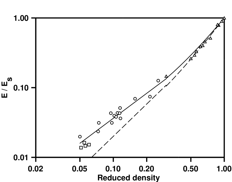
Figure 12

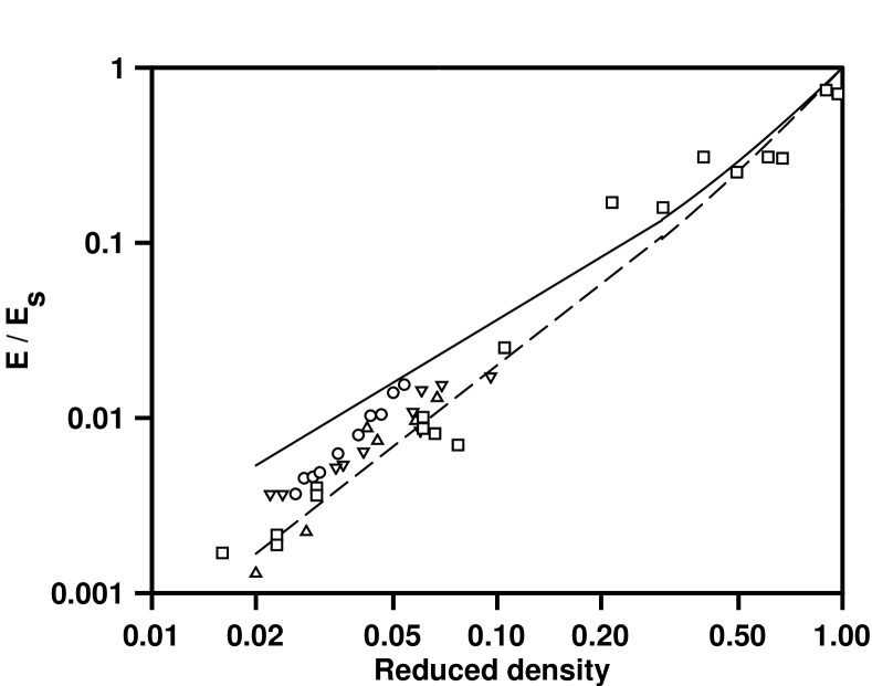
Figure 13

Figure 12: Young’s modulus of foamed glasses with closed cells. The data is from Morgan et al [32] ($\Box$), Zwissler and Adams [33] ($\circ$) ($E_{s}$=69 GPa [4]) and Walsh et al [36] ($\triangle$) ($E_{s}$=75 GPa). The solid line (——) corresponds to the closed-cell Voronoi tessellation. Results for the closed-cell GRF model (– – –) are shown for comparison.

Figure 13: Young’s modulus of closed cell polymer foams. The data is for extruded polystyrene [35] ($\circ$, $E_{s}$=1.4 GPa and $\rho_{s}$=1050 Kg/m³), polystyrene beads [9] ($\triangle$, $E_{s}$=3.0 GPa and $\rho_{s}$=1100 Kg/m³) expanded polystyrene [34] ($\Box$, $E_{s}$=2.65 GPa and $\rho_{s}$=1020 Kg/m³) and for low-density polyethylene [37] ($\bigtriangledown$). The solid (——) and dashed lines (– – –) correspond to the closed cell Voronoi tessellation and Gaussian random field models.

7 Discussion and Conclusion

We have used the finite element method to estimate the Young’s modulus of realistic random models of isotropic cellular solids. At low densities, the results can be described by the scaling relation $E/E_{s}=C(\rho/\rho_{s})^{n}$, where the parameters are reported in the text. At moderate to high densities, the results were described by Eq. (10). The equations used to describe the data are chosen to provide a reasonable fit, and consequently the fitting parameters do not have clear physical significance. It would be ideal to resolve the modulus into components from edge-bending and plate-stretching. However, the non-linear interaction between arbitrarily shaped cells and deformation makes this task impossible in all but the simplest of models.

All our results were obtained using a solid Poisson’s ratio of $\nu_{s}=0.2$. It has recently been shown [31] that the Young’s modulus only varies by around 2 % for $0<\nu_{s}<0.5$ indicating that our results are valid for all usual values of the solid Poisson’s ratio. The fitting relations we have derived can be used to predict the properties of cellular materials that have a microstructure similar to one of the models, and can be useful for interpreting experimental data.

Our results for closed-cell Voronoi tessellations were in general agreement with earlier studies on the tetrakaidecahedral foam, i.e., $E/E_{s}\approx\frac{1}{3}(\rho/\rho_{s})$ as $(\rho/\rho_{s})\to 0$ [5]. The actual exponent was $n=1.19$ which is greater than the value $n=1$ obtained for single-cell models and scaling arguments [Eq. (4), $\phi<1$]. If more than 70 % of of the cell faces are removed, the Young’s modulus exponent increased to $n=2$, indicating that edge bending becomes the dominant mechanism of deformation.

The closed-cell random field model, with curved cell walls, showed a significantly greater density dependence than the Voronoi tessellation (with exponent $n\approx 1.5$). Although the minimum density at which we were able to measure properties was $(\rho/\rho_{s})\approx 0.15$, the data showed no evidence of adopting a linear decay for $(\rho/\rho_{s})\to 0$, as suggested by theory.

The semi-empirical closed-cell theory given in Eq. (4) was found to not be applicable to the models studied here, since the low edge fractions ($\phi<0.5$) caused the equation to exceed known upper bounds on the Young’s modulus. Moreover, attempts to describe the deformation of closed or partially closed cellular materials in terms of a bending (exponent $n=2$) and plate stretching (exponent $n=1$) component were not successful. Instead, our results indicate that these mechanisms combine non-linearly and are best represented by a non-integer power law. Variational upper bounds, and other predictions for random closed cell foams, were found to significantly over-estimate the Young’s moduli of the models. Therefore numerical simulation must be relied on for accurate predictions.

In this study, we have shown that it is important to consider large-scale (multi-cellular) models of random cellular solids in order to obtain realistic elastic properties. While the modulus of the closed cell Voronoi tessellation can be approximately described by a single cell of the tetrakaidecahedral model, it is not possible to model the effect of missing faces and irregular cells with curved walls using single-cell models. Our results are consistent with experimental data, and show a more complex density dependence than predicted by conventional theories based on scaling arguments and periodic cell models. Our results focus on the effect of multi-cellular disorder, rather than local characteristics (e.g., distribution of mass between cell edges and walls) of cellular materials, for the following reasons. First, it is difficult to simultaneously model the local and global variables with finite computational power, and second, study of single cell models probably provides a more fruitful route to understanding the influence of local cell-character on the overall properties. We believe that the results of both approaches may be beneficially combined.

Acknowledgements— A.R. thanks the Fulbright Foundation and Australian Research Council for financial support. We also thank the Partnership for High-Performance Concrete program of the National Institute of Standards and Technology for partial support of this work.

References

- [1]
- [2] Gibson, L. J. and Ashby, M. F., Cellular solids: Structure and properties, Pergamon Press, Oxford, 1988.
- [3] Gibson, L. J. and Ashby, M. F., Proc. Roy. Soc. Lond. A, 1982, 382, 43–59.
- [4] Green, D. J., J. Am. Ceram. Soc., 1985, 68(7), 403.
- [5] Renz, R. and Ehrenstein, G. W., Cellular Polymers, 1982, 1, 5–13.
- [6] Simone, A. E. and Gibson, L. J., Acta Mater., 1998, 46(6), 2139–2150.
- [7] Grenestedt, J. L. and Tanaka, K., Scripta Mater., 1999, 40(1), 71–77.
- [8] Grenestedt, J. L., Int. J. Solids Struct., 1999, 36, 1471–1501.
- [9] Mills, N. J. and Zhu, H. X., J. Mech. Phys. Solids, 1999, 47, 699–695.
- [10] Silva, M. J., Hayes, W. C. and Gibson, L. J., Int. J. Mech. Sci., 1997, 37(11), 1161–1177.
- [11] Silva, M. J. and Gibson, L. J., Int. J. Mech. Sci., 1997, 39(5), 549–563.
- [12] Garboczi, E. J., Phys. Rev. B, 1989, 39, 2472–2475.
- [13] Grenestedt, J. L., J. Mech. Phys. Solids, 1998, 46(1), 29–50.
- [14] Roberts, A. P. and Knackstedt, M. A., J. Mater. Sci. Lett., 1995, 14, 1357–1359.
- [15] Garboczi, E. J. and Day, A. R., J. Mech. Phys. Solids, 1995, 43, 1349–1362.
- [16] Stoyan, D., Kendall, W. S. and Mecke, J., Stochastic geometry and its applications, 2nd edn., Wiley, Chichester, 1995.
- [17] Berk, N. F., Phys. Rev. Lett., 1987, 58, 2718–2721.
- [18] Christensen, R. M., J. Mech. Phys. Solids, 1986, 34(6), 563–578.
- [19] Torquato, S., Appl. Mech. Rev., 1991, 44, 37–76.
- [20] Hashin, Z. and Shtrikman, S., J. Mech. Phys. Solids, 1963, 11, 127–140.
- [21] Milton, G. W. and Phan-Thien, N., Proc. Roy. Soc. London A, 1982, 380, 305–331.
- [22] Cook, R., Malkus, D. and Plesha, M., Concepts and Applications of Finite Element Analysis, J. Wiley and Sons, New York, 1989.
- [23] Hashin, Z., J. Appl. Mech., 1983, 50, 481–505.
- [24] Garboczi, E. J., 1998, IST Internal Report 6269, available at http://ciks.cbt.nist.gov/garboczi/, Chapter 2.
- [25] Christensen, R. M., Mechanics of composite materials, Wiley, New York, 1979.
- [26] Van der Burg, M. W. D., Shulmeister, V., Van der Geissen, E. and Marissen, R., J. Cell. Plast., 1997, 33, 31–54.
- [27] Weaire, D. and Fortes, M. A., Adv. Phys., 1994, 43(6), 685–738.
- [28] Roberts, A. P. and Knackstedt, M. A., Phys. Rev. E, 1996, 54, 2313–2328.
- [29] Roberts, A. P., Phys. Rev. E, 1997, 55, 1286–1289.
- [30] Roberts, A. P. and Garboczi, E. J., J. Mech. Phys. Solids, 1999, 47(10), 2029–2055.
- [31] Garboczi, E. J. and Roberts, A. P., Computations of the linear elastic properties of random porous materials with a wide variety of microstructure, 2000, in preperation.
- [32] Morgan, J. S., Wood, J. L. and Bradt, R. C., Mater. Sci. Eng., 1981, 47(1), 37–42.
- [33] Zwissler, J. G. and Adams, M. A., in Bradt, R. C., Evans, A. G., Hasselman, D. P. H. and Lange, F. F., eds., Fracture Mechanics of Ceramics, vol. 6, Plenum Press, New York, 1983 pp. 211–241.
- [34] Baxter, S. and Jones, T. T., Plast. Polym., 1972, 40, 69–76.
- [35] Chan, R. and Nakamura, M., J. Cell. Plast., 1969, 5, 112–118.
- [36] Walsh, J. B., Brace, W. F. and England, A. W., J. Am. Ceram. Soc., 1965, 48(12), 605–608.
- [37] Clutton, E. Q. and Rice, G. N., in 34th Annual Technical Conference Proceedings, RAPRA Technology, Shrewsbury, 1991 pp. 99–107.
- [38]