Mobility Edge in Aperiodic Kronig-Penney Potentials with Correlated Disorder: Perturbative Approach

Abstract

It is shown that a non-periodic Kronig-Penney model exhibits mobility edges if the positions of the scatterers are correlated at long distances. An analytical expression for the energy-dependent localization length is derived for weak disorder in terms of the real-space correlators defining the structural disorder in these systems. We also present an algorithm to construct a non-periodic but correlated sequence exhibiting desired mobility edges. This result could be used to construct window filters in electronic, acoustic, or photonic non-periodic structures.

The Kronig-Penney model has been widely used to explore the characteristics of electrons in a periodic potential, as this model provides one with perhaps the simplest instance of Bloch states. This model is also used systematically to provide estimates of the bandwidths in semiconductor superlattices with high reliability. [1] The Kronig-Penney model and its relation with superlattices has also been used in recent times to provide an implementation of the physics of random and quasi-periodic systems, [2] and interesting experiments have been reported on arrangements such as the well-known Fibonacci sequences. [3] It is because of its importance and wide applicability that we focus our attention on the Kronig-Penney model. We will demonstrate that the aperiodic model with constant scattering potential but random spacings yields mobility edges if the disorder has long-range correlations, in sharp contrast to the situation for white noise potentials.

The Kronig-Penney model in this study is given by a 1D chain of delta-function scatterers with amplitude $U_{n}$ and centered at points $z_{n}$. The Schrödinger equation for a particle moving in this random potential has the form,

$$(\hbar^{2}/2m)\psi^{\prime\prime}(z)+E\psi(z)=\sum_{n=-\infty}^{\infty}U_{n}\psi(z_{n})\delta(z-z_{n})\,.$$ (1)

This is equivalent to the discrete equation,

$$\begin{array}[]{cc}&\sin\mu_{n-1}\psi_{n+1}+\sin\mu_{n}\psi_{n-1}=\\ &\left[\sin(\mu_{n}+\mu_{n-1})+(U_{n}/q)\sin\mu_{n-1}\sin\mu_{n}\right]\psi_{n},\end{array}$$ (2)

where $\psi_{n}\equiv\psi(z_{n})$, $\mu_{n}=q(z_{n+1}-z_{n})$, $q=\sqrt{E}$, and the energy is measured in units where $\hbar^{2}/2m=1$. The linear relation (2) between $\psi_{n-1}$, $\psi_{n}$, and $\psi_{n+1}$, can be easily arrived at by integrating Eq. (1) in the vicinity of sites ${n-1}$, $n$, and $n+1$, and substituting the amplitudes for the various constants in the piece-wise zero-potential regions between the scatterers. If the site potential is different from a delta function, a linear relation similar to Eq. (2) can be obtained using a general method described in Ref. [4]. Therefore, Eq. (2) can be considered as a rather generic relation for 1D chains with potential scatterers. We focus here on a sequence of scatterers of equal amplitude, $U_{n}\equiv U$, but with varying positions, i.e. the case of ‘structural’ or ‘positional’ disorder. An obvious experimental realization of this model is a semiconductor superlattice with fluctuating period.

The case of compositional disorder, i.e., a periodic arrangement of sites, $z_{n}=n$, with random amplitude $U_{n}$, has been studied intensively during the last decade. The importance of short-range correlations was first explored recently, [5] and a ‘random dimer’ model was studied as a specific example. [6] Using this model, it was shown that short-range correlations in the infinite random sequence $\left\{U_{n}\right\}$ give rise to a discrete number of delocalized states as well as to some anomalies in transport properties. [7] The presence of such anomalies has been recently observed in experiments with GaAs-AlGaAs random-dimer superlattices. [8] Moreover, the non-trivial role of correlations in the formation of mobility edges has been pointed out by the study of localization in pseudorandom and incommensurate potentials. [9] In contrast, only relatively recently the role of long-range correlations in random potentials has received special attention. The interplay of long-range correlations and disorder has been shown to lead to the existence of a continuum of extended states in the energy spectrum and to the appearance of mobility edges.[10, 11] These edges have been shown to exist in experiments of microwave transmission in a single-mode waveguide with a random array of correlated scatterers,[12] and their possible relevance for metal-insulator transitions in 2D electron systems has been recently explored.[13]

Localization length for weak disorder. To calculate the localization length $l(E)$ in the case of structural disorder we use a Hamiltonian approach. [14] In this scheme, the discrete Schrödinger equation is replaced by a classical Hamiltonian map for coordinate $x_{n}$ and momentum $p_{n}$. For the case of Eq. (2), conjugate variables are introduced as, $\,x_{n}=\psi_{n}$ and $p_{n}=(x_{n}\cos\mu_{n-1}-x_{n-1})/\sin\mu_{n-1}$. Correspondingly, the discrete-time evolution of $x_{n}$ and $p_{n}$ is obtained from

$$\begin{array}[]{cc}p_{n+1}=(p_{n}\,+A_{n}\,x_{n})\cos\mu_{n}\,\,-\,\,x_{n}\sin\mu_{n},&\\ x_{n+1}=(p_{n}\,+A_{n}\,x_{n})\sin\mu_{n}\,\,+\,\,x_{n}\cos\mu_{n}\,.\end{array}$$ (3)

This map describes the behavior of a linear rotator subjected to non-periodic delta-kicks with amplitude $A_{n}=U_{n}/q$. Free rotation between kicks corresponds to free propagation between scatterers and each kick corresponds to scattering at each $\delta$-function potential. It is easy to check that the first equation in (3) is equivalent to (2), while the second is reduced to an identity after $p_{n}$ substitution.

In what follows we consider the case of weak disorder, assuming that the deviation of the scatterers from their positions in a periodic lattice is small, $|\delta_{n}|=q|z_{n}-n|\ll 1$. We can then expand trigonometric functions in (3) and up to second order in $\lambda_{n}=q(\delta_{n+1}-\delta_{n})$, obtain the approximate map for constant kick amplitude $A=U/q$,

$$\begin{array}[]{cc}p_{n+1}=\cos q\left[p_{n}(1-\frac{\lambda_{n}^{2}}{2})+x_{n}(A-\lambda_{n}-A\frac{\lambda_{n}^{2}}{2})\right]\\ -\sin q\left[p_{n}\lambda_{n}+x_{n}(1+A\lambda_{n}-\frac{\lambda_{n}^{2}}{2})\right],\\ x_{n+1}=\cos q\left[p_{n}\lambda_{n}+x_{n}(1+A\lambda_{n}-\frac{\lambda_{n}^{2}}{2})\right]\\ +\sin q\left[p_{n}(1-\frac{\lambda_{n}^{2}}{2})+x_{n}(A-\lambda_{n}-A\frac{\lambda_{n}^{2}}{2})\right].\end{array}$$ (4)

Note that since $\lambda_{n}\propto q=\sqrt{E}$, this expansion is valid only for low energies.

In order to extract the effect that comes only from the positional non-periodicity, it is convenient to eliminate the mean field associated with the constant amplitude $U$. This can be done by a canonical transformation of variables,

$$\begin{array}[]{cc}p_{n}=\alpha^{-1}\cos\phi\,P_{n}\,-\alpha\sin\phi\,X_{n}\,,&\\ x_{n}=\alpha^{-1}\sin\phi\,P_{n}\,+\alpha\cos\phi\,X_{n}\,.&\end{array}$$ (5)

The parameters of this transformation ($\alpha$ and $\phi$) are obtained from the condition that to zeroth order in $\lambda_{n}$ the dynamical map for $(P_{n},X_{n})$ be a simple rotation without kicks, i.e., $P_{n+1}^{(0)}=P_{n}^{(0)}\cos\gamma-X_{n}^{(0)}\sin\gamma$, and $X_{n+1}^{(0)}=P_{n}^{(0)}\sin\gamma+X_{n}^{(0)}\cos\gamma$. Applying this condition to Eqs. (5) and (4) we get after some algebra:

$$\begin{array}[]{cc}\phi=\frac{1}{2}q\,,\,\,\,\cos\gamma=\cos q+(A/2q)\sin q\,,\\ \alpha^{4}=1+2A/\left[2\sin q-A(1+\cos q)\right].\end{array}$$ (6)

It is clear that $\gamma$ plays the role of the Bloch number in the periodic Kronig-Penney model. [1] We can now rewrite the map (4) in terms of variables $(P_{n},X_{n})$ and angle $\gamma$,

$$\begin{array}[]{cc}P_{n+1}=\left(1-\lambda_{n}^{2}/2\right)(P_{n}\cos\gamma-X_{n}\sin\gamma)&\\ -\lambda_{n}\alpha^{2}(P_{n}\sin\gamma+X_{n}\cos\gamma),\\ X_{n+1}=\left(1-\lambda_{n}^{2}/2\right)(P_{n}\sin\gamma+X_{n}\cos\gamma)&\\ +\lambda_{n}\alpha^{-2}(P_{n}\cos\gamma-X_{n}\sin\gamma).\end{array}$$ (7)

Following our previous approach,[11] it is convenient to introduce action-angle variables for map (7),

$$P_{n}=R_{n}\sin\theta_{n},\,\,\,\,X_{n}=R_{n}\cos\theta_{n}\,.$$ (8)

The inverse localization length for the original quantum model Eq. (1) (or equivalently, the Lyapunov exponent for the dynamical map in (3)), can be expressed in terms of the ratio $R_{n+1}/R_{n}$ (see details in Ref. [14]),

$$l^{-1}(E)=\left\langle{\ln\frac{\psi_{n+1}}{\psi_{n}}}\right\rangle = \left\langle{\ln\frac{X_{n+1}}{X_{n}}}\right\rangle=\frac{1}{2}\left\langle{\ln\frac{R_{n+1}^{2}}{R_{n}^{2}}}\right\rangle\,.$$ (9)

Here, angular brackets stand for the average over sites (kicks), so that, $\left\langle{...}\right\rangle=\lim_{N\rightarrow\infty}\,\frac{1}{N}\sum_{n=1}^{N}\left(...\right)$. Using the map (7) we can calculate the ratio $R_{n+1}/R_{n}$ as

$$\begin{array}[]{cc}\left(R_{n+1}/R_{n}\right)^{2}=1-U\lambda_{n}\sin\left[2\left(\theta_{n}-\gamma\right)\right]/(q\sin\gamma)\\ +\lambda_{n}^{2}\left[\alpha^{-4}\sin^{2}(\theta_{n}-\gamma)+\alpha^{4}\cos^{2}(\theta_{n}-\gamma)-1\right]\end{array}$$ (10)

The fact that the ratio $R_{n+1}/R_{n}$ is close to unity for small $\lambda_{n}$ is what motivated switching from the variables ($p_{n},x_{n}$) to ($P_{n},X_{n}$) using (5). The logarithm in (9) can be expanded as $\ln(1+x)\approx x-x^{2}/2$, and, up to second order in $\lambda_{n}$, the average is performed over the unperturbed motion given by the $(P_{n}^{(0)},X_{n}^{(0)})$ variables. Since this motion is a free rotation (in the old variables it is a rotation with periodic kicks), the angle variable $\theta_{n}$ is clearly distributed uniformly within the interval $[0,2\pi]$. One then obtains that $\left\langle\sin^{2}\theta_{n}\right\rangle=\left\langle{\cos^{2}\theta_{n}}\right\rangle=1/2$, and

$$l^{-1}(E)=\frac{\left\langle{\lambda_{n}^{2}}\right\rangle U^{2}}{8q^{2}\sin^{2}\gamma}-\frac{U}{q\sin\gamma}\left\langle{\lambda_{n}\sin[2(\theta_{n}-\gamma)]}\right\rangle\,.$$ (11)

The first term in (11) gives the inverse localization length in an uncorrelated random potential. In this Born approximation, it is proportional to the variance $\left\langle\lambda_{n}^{2}\right\rangle$ and to the squared amplitude of the scattering potential, $U^{2}$. Since $\left\langle{\lambda_{n}^{2}}\right\rangle\propto q^{2}$, the factor $q^{2}$ disappears and the only energy dependence is due to the factor $\sin^{2}\gamma$ in the denominator. At the edges of the allowed zones $\sin\gamma=0$, and here the localization length $l(E)$ approaches zero. A similar enhancement of localization in the vicinity of the band edges [15, 16] has stimulated the study of photonic-band-gap materials in the last decade.

The second term in (11) describes the contribution of correlations in the scattering potential. To calculate explicitly the correlator $\left\langle{\lambda_{n}\sin[2(\theta_{n}-\gamma)]}\right\rangle$, one needs the recursion relation for the angle variable $\theta_{n}$. Since this correlator already contains a factor $\lambda_{n}$, only linear terms in the recursion relation are needed from Eqs. (7) and (8), so that $\theta_{n}=\theta_{n-1}-\gamma-\lambda_{n-1}\left[\alpha^{2}-U\sin^{2}(\theta_{n-1}-\gamma)/(q\sin\gamma)\right]$. The correlator $\left\langle{\lambda_{n}\sin[2(\theta_{n}-\gamma)]}\right\rangle$ can be written as a Fourier series in Bloch number $\gamma$, where the dimensionless correlators $\xi(k)$ are the Fourier coefficients,[11]

$$\left\langle{\lambda_{n}\sin[2(\theta_{n}-\gamma)]}\right\rangle=-\frac{Uq\Delta^{2}}{2\sin\gamma}\sum_{n=1}^{\infty}\xi(n)\cos(2\gamma n)\,.$$ (12)

Here $\Delta^{2}=\left\langle{\Delta_{n}^{2}}\right\rangle$, with $\xi(k)=\left\langle{\Delta_{n+k}\Delta_{n}}\right\rangle/\Delta^{2}$, and $\Delta_{n}=\delta_{n+1}-\delta_{n}$. Note that the localization length is determined by the statistical properties of the sequence of relative displacements $\Delta_{n}$, and not by the displacements $\delta_{n}$ themselves.

Substituting the correlator (12) into (11) we get the final result for the inverse localization length,

$$\frac{1}{l(E)}=\frac{U^{2}\Delta^{2}}{8\sin^{2}\gamma}\varphi(\gamma),\,\,\varphi(\gamma)=1+2\sum_{n=1}^{\infty}\xi(n)\cos(2\gamma n).$$ (13)

This formula has the same structure as that obtained for a tight-binding (and the corresponding Kronig-Penney) model with random amplitudes $U_{n}$, but equidistant sites ($z_{n}=n$). [11, 12] These three different models have a different dependence on energy via the factors $q^{2}$ and $\sin^{2}\gamma$. The present case exhibits the weakest dependence of the localization length on energy within the allowed zone since a factor $q^{2}=E$ appears in other cases but not here. This property should be favorable for the experimental observation of mobility edges in superlattices with positional disorder.

Correlations and mobility edge. If the sequence of random displacements $\Delta_{n}$ is uncorrelated, $\xi(k)=0$, the localization length is given by the first term in (13). In the opposite limit of a completely correlated sequence, $\xi(k)=$const., the displacements are independent on the site number, $\delta_{n}=\delta_{0}$, giving a regular sequence with period $1+\delta_{0}$, and extended states, $l^{-1}=0$, for all energies. A smooth transition between these two limits can be described by an exponential function, $\xi(k)=\exp(-k/k_{0})$, where $k_{0}$ is a correlation radius. Substituting this form into (13) one obtains

$$l^{-1}(E)={\frac{U{{}^{2}}\Delta^{2}}{8\,{\sin^{2}\gamma}}\,}{\frac{{\sinh{(1/k_{0})}}}{{\cosh(1/k_{0})-\cos(2\gamma)}}}\,.$$ (14)

For any finite $k_{0}$ all states are localized. Only in a periodic lattice ($k_{0}=\infty$) does the inverse localization length (14) vanish and the states become delocalized. This localization-delocalization transition occurs simultaneously for all energies, and a mobility edge does not appear in the spectrum. This conclusion is valid for arbitrary amplitude of the scattering potential $U$.[17] A discrete number of delocalized states can in fact appear if the binary correlator $\xi(k)$ oscillates with exponentially decaying amplitude.[18] This can be obtained from (14), if the correlation radius $k_{0}$ is allowed to take complex values. On the other hand, a mobility edge may appear if correlations decay not exponentially but according to a power law.[10, 11, 12] We show numerically below that mobility edges exist if, e.g., $\xi(k)\propto 1/k$.

Designed mobility edges. In a real (or numerical) experiment one needs to know explicitly the displacements $\delta_{n}$ which provide a desirable dependence $l(E)$. This leads us to the ‘inverse problem’ in the theory of localization. The solution would give us in general a random scattering potential $\{U_{n},\delta_{n}\}$ through the dependence $l(E)$. In the present case of positional disorder, $U_{n}=U$, we need to calculate only the relative displacements. One can explicitly evaluate the correlator $\xi(k)$ as the Fourier coefficient,

$$\xi(k)=\frac{2}{\pi}\int_{0}^{\pi/2}\varphi(\gamma)\cos(2k\gamma)d\gamma\,,$$ (15)

where the energy dependence of $\varphi(\gamma)=8\sin^{2}\gamma/(U^{2}\Delta^{2}l(E))$, is assumed to be known. The energy $E=q^{2}$ is expressed through $\gamma$ via the dispersion relation in (6). It is easy to check that the binary correlator of a sequence $(\Delta_{n}/\Delta)=\sum_{k=-\infty}^{\infty}\beta(k)\,Z_{n+k}\,$, coincides with $\xi(k)$ if $Z_{k}$ are random numbers with zero mean and unit variance, and where the function $\beta(k)$ is given by [11, 12, 19]

$$\beta(k)=\frac{2}{\pi}\int_{0}^{\pi/2}\sqrt{\varphi(\gamma)}\cos(2k\gamma)d\gamma\,.$$ (16)

Once the relative displacements $\Delta_{n}$ are known, a sequence of absolute displacements can be easily calculated, setting $\delta_{0}=0$, for example, and then $\delta_{1}=\Delta_{0},$ $\delta_{2}=\Delta_{0}+\Delta_{1},$ $\ldots$ , $\delta_{n}=\sum_{k=0}^{n-1}\Delta_{k}$. This procedure allows the calculation of displacements $\delta_{n}$ for any energy dependence of the localization length $l(E)$, including situations with mobility edges. Appropriately correlated elements may be used for fabrication of effective filters of electrical or optical signals, even if the system is not periodic. [20] The bandwidth of a filter can be made arbitrarily wide or narrow depending on the statistical properties of the random sequence used (via the function $\beta(k))$.

Numerical examples. In order to examine our predictions, we construct explicit random sequences $\{\delta_{n}\}$ for which the function $\varphi(\gamma)$ in (13) has four mobility edges at $\gamma_{i}=0.2\pi i,\,\,i=1,\dots,4$. The positions of the mobility edges are chosen within the interval $0<\gamma<\pi$, symmetrically about $\gamma=\pi/2$. Via relation (6), the position of the mobility edges on the axis $q/\pi$ are given by 0.326, 0.478, 0.649, and 0.850, for the mean field amplitude $U=0.7$. In the ideal lattice with the same strength of the potential, the first allowed band lies between $q_{l}/\pi\approx 0.26$ ($\gamma=0$) and $q_{r}/\pi\approx 1$ ($\gamma=\pi$). Numerical data are given for two complimentary situations $\varphi_{1,2}(\gamma)$: $\varphi_{1}$ vanishes (i.e. $l(E)=\infty$ and states are delocalized) in the region $\gamma\in(0,\gamma_{1})\cup(\gamma_{2},\gamma_{3})\cup(\gamma_{4},\pi)$; while $\varphi_{2}$ vanishes in the complementary region $\gamma\in(\gamma_{1},\gamma_{2})\cup(\gamma_{3},\gamma_{4})$. Outside these regions, the function $\varphi_{1,2}(\gamma)$ is a constant defined by the normalization condition $\xi_{1,2}(0)=1$. From Eq. (15), we get that because of the presence of sharp mobility edges the correlators (Fourier components of a discontinuous function) decay slowly:

$$\xi_{1}(k)=-1.5\,\xi_{2}(k)=$$ (17)

$$(5/2\pi k)\left[\sin(0.8\pi k)-\sin(0.4\pi k)\right].$$ (18)

FIG. 1.: Inverse localization length for band with four mobility edges, three regions of extended states, and different amplitude of disorder: circles ($\circ$), $\Delta=0.05$; crosses ($\times$), $\Delta=0.15$. Solid lines show Eq. (13) for $\Delta=0.05$. Inset shows $N=10^{3}$ sites averaged over only 100 samplings.

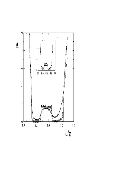
FIG. 2.: Results for complementary system to Fig. 1, with four mobility edges but only two regions of extended states. Lines through circles ($\Delta=0.05$) and crosses ($\Delta=0.15$) are guides to the eye.

We show the corresponding data in Fig. 1 and 2 for $U=0.7$. The analytical dependence (13) for the dimensionless inverse localization length $\Lambda=8/l(E)U^{2}\Delta^{2}$ is shown by the full lines for $\Delta=0.05\,$ in the figures. Numerical data are obtained for a large sample size $N=10^{6}$, with two amplitudes of disorder, $\Delta=0.05$ (circles) and $\Delta=0.15$ (crosses). The insets show results for a much shorter sample, $N=1000$, with additional average over 100 different realizations of disorder but the same correlations. One can see that for small disorder, $\Delta=0.05$, Eq.(13) describes the numerical results very well, with only minor deviations close to the onset of mobility $q_{i}$ and band edges, $q_{l,r}$ . Notice that Eq.(13) is excellent at giving the mobility edges at the prescribed energies, which proves its usefulness, and breadth of applicability.

This work was supported by CONACyT (Mexico) Grants No. 26163-E and 28626-E, and by the US Department of Energy Grant No. DE-FG02-91ER45334. AAK is grateful for a Rufus Putnam Fellowship from Ohio University.

REFERENCES

- [1] See, e.g, G. Bastard, Wave mechanics applied to semiconductor heterostructures (Halsted Press, New York, 1988).
- [2] M. Kohmoto, et al., Phys. Rev. Lett.50, 1870 (1983); M. Kohmoto, Phys. Rev. B34, 5043 (1986); S. Das Sarma, et al., Phys. Rev. Lett.56, 1280 (1986); L.N. Gumen and O.V. Usatenko, Phys. Stat. Sol. 162, 387 (1990); U. Kuhl and H.-J. Stöckmann, Phys. Rev. Lett.80, 3232 (1998).
- [3] R. Merlin, K. et al., Phys. Rev. Lett. 55, 1768 (1985).
- [4] A. Sánchez, et al., Phys. Rev. B 49, 147 (1994).
- [5] J.C. Flores, J. Phys.: Condens. Matter 1, 8471 (1989); A. Crisanti, et al., ibid 1, 9505 (1989).
- [6] D. Dunlap, et al., Phys. Rev. Lett. 65, 88 (1990); P. Phillips and H.-L. Wu, Science 252, 1805 (1991).
- [7] A. Bovier, J.Phys. A: Math. Gen., 25, 1021 (1992); H.-L. Wu et al., Phys. Rev.B 45, 1623 (1992); S.N. Evangelou et al., Phys. Lett. A 164, 456 (1992); P.K. Datta et al., Phys. Rev. B 47, 10727 (1993); E. Diez et al., Phys. Rev. B 50 (1994); E. Diez, et al., Solid St. Electr. 40, 433 (1996); N. Zerki, et al., Phys. Lett. A 234, 391 (1997).
- [8] V. Bellani, et al., Phys. Rev. Lett. 82, 2159 (1999).
- [9] S. Das Sarma, et al., Phys. Rev. Lett. 61, 2144 (1988); A. Crisanti, J. Phys. A: Math. Gen. 22, L681 (1989); R. Farchioni, et al., J.Phys.: Condens. Matter 5, B13 (1993).
- [10] F. Moura and M. Lyra, Phys. Rev. Lett. 81, 3735 (1998); ibid 84, 199 (2000); Physica A, 266, 465 (1999).
- [11] F.M. Izrailev and A.A. Krokhin, Phys. Rev. Lett. 82, 4062 (1999); A.A. Krokhin and F.M. Izrailev, Ann. Phys. (Leipzig), 8, Spec. Issue, S1, 153 (1999).
- [12] U.Kuhl, et al., Appl. Phys. Lett., 77, 633 (2000).
- [13] V.V. Flambaum and V.V. Sokolov, Phys. Rev. B60, 4529 (1999).
- [14] F.M. Izrailev, et al., Phys. Rev. B 52, 3274 (1995); F.M. Izrailev, et al., Journ. Phys. A: Math. Gen. 31, 5263 (1998).
- [15] S. John, Phys. Rev. Lett. 58, 2486 (1987).
- [16] A.R. McGurn, et al., Phys. Rev. B 47, 13120 (1993).
- [17] A. Crisanti, et al., Phys. Rev. A 39, 6491 (1989).
- [18] J.S. Denbigh and N. Rivier, J. Phys. C 12, L107 (1979).
- [19] We are thankful to V. Sokolov for the suggestion concerning this algorithm and to I. Herbut for sending us (prior to submission) the preprint cond-mat/0007266, where Eq. (16) has been derived independently.
- [20] For classical waves see, e.g., G. Samelsohn, S.A. Gredeskul, and R. Mazar, Phys. Rev. E60, 6081 (1999), and references therein.